Force calculation on walls and embedded particles in
Multi-Particle Collision Dynamics simulations

Abstract

Colloidal solutions posses a wide range of time and length scales, so that it is unfeasible to keep track of all of them within a single simulation. As a consequence some form of coarse-graining must be applied. In this work we use the Multi-Particle Collision Dynamics scheme. We describe a particular implementation of no-slip boundary conditions upon a solid surface, capable of providing correct forces on the solid bypassing the calculation of the velocity profile or the stress tensor in the fluid near the surface. As an application we measure the friction on a spherical particle, when it is placed in a bulk fluid and when it is confined in a slit. We show that the implementation of the no-slip boundary conditions leads to an enhanced Enskog friction, which can be understood analytically. Because of the long-range nature of hydrodynamic interactions, the Stokes friction obtained from the simulations is sensitive of the simulation box size. We address this topic for the slit geometry, showing that that the dependence on the system size differs very much from what is expected in a 3D system, where periodic boundary conditions are used in all directions.

I Introduction

The existence of a huge range of time and length-scales, spanning between mesoscopic colloidal particles and microscopic solvent particles, constitutes a severe problem in numerical simulations. Hybrid schemes have been developed, in which different coarse-grained approaches are used to describe solvent molecules and colloids. Prominent in the class of solvent models is Multi-Particle Collision Dynamics (MPCD), originally proposed by Malevanets and Kapral Malevanets and Kapral (1999), which has proved to be very effective in simulating Newtonian fluids out of equilibrium. For a review see Gompper and et al. (2009).
The interaction between solvent molecules and colloids may be described in several ways, mimicking the various boundary conditions (BC) in use in continuum descriptions. The molecular origins of these boundary conditions can be very complex Boquet and J.L. Barrat (1994); Lauga et al. (2005), but for most colloidal applications, simple no-slip BC are sufficient for modeling experimental conditions. In this paper we discuss a way to impose such boundary conditions in MPCD simulations of liquids containing dissolved colloids.

MPCD simulations consist of two alternating steps: the streaming step (where Newton’s equations of motions for non-interacting particles are solved) and the collision step (where the fluid is coarse-grained). The no-slip BC involve both steps. In particular, during the collision step, virtual particles (VP) are inserted in the regions of the MPCD box occupied by walls or colloids.This idea has already been used in Lamura et al. (2001); R.G. Winkler and C.C. Huang (2009); I.O. Gotze et al. (2007); M.T. Downton and Stark (2009). In this paper, we will provide additional insight in this method, analyzing not only the velocity profiles nearby solid planar walls, but also discussing the contributions of the VP to the forces exerted by the solvent on the solid boundaries. Such forces determine the drag forces experienced by the colloids and thereby regulate the colloids’ dynamics. A recent interesting work discussing these techniques in the implementation of mixed stick-slip boundary conditions can be found in Whitmer and Luijten (2010).
The second topic we treat is the role of finite-size effects (FSE) of the simulation box. In molecular dynamics simulations it is common practice to use periodic BC to mimic an infinite system. However, due to the long-range nature of the hydrodynamic interactions, quantities such as the Stokes friction can still be affected by the system size even when equilibrium properties are well reproduced Dünweg and Kremer (1993). The use of periodic BC implies a set of images of the colloidal particle, so that they all together form a periodic grid. The problem of slow flow through a 3D periodic array of spheres has been treated by Zick and Homsy (1982), while in Dünweg and Kremer (1993) FSE are studied for a chain of beads in a solvent. In both works, periodic BC are assumed along all three directions.
When confining walls are present in one direction, and periodic BC in the others (such as in the simulation of a slit geometry), the problem of the FSE has been addressed only recently in S.C. Hohale and Khare (2008) for slip BC, using molecular dynamics simulations, and in Bhattacharya (2008) for no-slip BC, using continuum models. Our results, obtained with coarse-grained simulations, are qualitatively in agreement with such previous works for the friction in the direction parallel to the walls. Furthermore we also discuss the friction in the direction perpendicular to the walls, which is missing in Bhattacharya (2008); S.C. Hohale and Khare (2008). For both the parallel and perpendicular friction strong differences emerge with respect to the case of a cubic box with periodic BC in all directions.

The structure of this paper is as follows: in section  II the simulation technique is introduced, with particular emphasis on the use of the VP during the collision step; in section III, we validate the model through the study of the Poiseuille flow in a slit, for which the theory is known. In particular we calculate the forces exerted by the solvent on the solid walls through two independent methods, once by using the VP and once using the stress tensor for a MPCD fluid near planar boundaries. In section IV, we compute the friction on a single sphere in bulk. Because of the VP, the local Brownian friction is increased, and we provide an Enskog-like model to predict such an effect. In section V the colloidal particle is confined in a slit, and we measure the friction as a function of the lateral size of the walls, while keeping fixed the separation between the walls. Final remarks and observations are in section VI.

II Simulation technique

In the present application, Multi-Particle Collision Dynamics (MPCD) is a hybrid simulation scheme, in which a coarse-grained approach is used to describe the solvent variables, while an atomistic description is adopted for the solvent-solute and for the solute-solute interactions. The dynamics of the system is made up of two steps: streaming and collision. In the streaming step, the position and velocity of each particle is propagated for a time $\delta t$ by solving Newton’s equations of motion. In the collision step the fluid is subdivided into cubic cells of side $a$. Then a stochastic rotation of the particles velocities, relative to the center of mass motion of the relevant cell, is performed according to the formula:

$$\bm{V}_{i}(t)=\bm{u}+\bm{\Omega}\{\bm{v}_{i}(t)-\bm{u}\},$$ (1)

where $\bm{u}$ is the mean velocity of the particles within a cell and $\bm{\Omega}$ is a matrix which rotates velocities by a fixed angle (in this work $\alpha~{}=~{}\pi/2$) around a randomly oriented axis. Through the stochastic rotation of the velocities, the solvent particles can efficiently exchange momentum without introducing direct forces between them during the streaming step. As the collision step conserves mass, linear momentum and energy, the correct hydrodynamic behavior is obtained on the mesoscopic scale Malevanets and Kapral (1999, 2000), as long as a shifted-grid procedure is included in order to enforce Galilean invariance Ihle and Kroll (2001). When colloids are present, Newton’s equations of motion are solved also for them J.T. Padding and A.A. Louis (2006). Special care must be used if no-slip boundary conditions (BC) are applied on the colloidal surface and on the confining walls. In this case, in fact, we must couple colloids and walls to the solvent during the collision step too. This is achieved by means of virtual particles (VP). The implementation of the no-slip BC is described in the following.
Streaming step: when a MPCD particle crosses the colloid (or wall) surface, it is moved back to the impact position. Then a new velocity is extracted from the following distributions for the tangent ($v_{t}$) and the normal components ($v_{n}$) of the velocity, with respect to the surface velocity:

$$p(v_{n})=\frac{mv_{n}}{k_{B}T}exp\left(-mv_{n}^{2}/2k_{B}T\right),$$ (2)

$$p(v_{t})=\sqrt{m/2\pi k_{B}T}exp\left(-mv_{t}^{2}/2k_{B}T\right),$$ (3)

where $m$ is the mass of the solvent particle, $k_{B}$ Boltzmann’s constant, and $T$ the temperature of the system. Once the velocity has been updated, the particle is displaced for the remaining part of the integration time step.
Collision step: VP are inserted randomly in those parts of the system which are physically occupied by the colloid or by the walls (in sufficiently thick layers behind the interfacial positions). The VP density matches the MPCD solvent density $\gamma$, while their velocities $\bm{v}_{i}^{VP}$ are obtained from a Maxwell-Boltzmann distribution, whose average velocity is equal to the velocity of the colloid surface or to the velocity of the walls, and the temperature is the same as in the solvent. According to their coordinates, VP are sorted into the grid cells. During the collision step, the average velocity of the center of mass of the cell is computed as

$$\bm{u}=\frac{\overset{n_{MPCD}}{\sum_{i=1}}\bm{v}_{i}(t)+\overset{n_{VP}}{\sum_{i=1}}\bm{v}_{i}^{VP}(t)}{n_{MPCD}+n_{VP}},$$ (4)

where $n_{MPCD}$ and $n_{VP}$ respectively are the number of MPCD particles and the number of VP belonging to the same cell. Finally velocities of both MPCD and VP belonging to the same cell are rotated according to the rule given in Eq.(1).

Due to the exchange of momentum between the solvent and the colloidal particle, the force exerted upon the latter may be expressed as: $\bm{F}=\bm{f}_{s}+\bm{f}_{c}$, where $\bm{f}_{s}$ and $\bm{f}_{c}$ are the forces during the streaming step and the collision step, respectively. The former can be calculated as:

$${\bf{f}}_{s}=-\frac{1}{\delta t}\overset{Q}{\sum_{i=1}}\Delta{\bf{P}}_{i}^{MPCD},$$ (5)

where $Q$ is the number of MPCD particles which have crossed the surface of the colloid between two collision steps and $\Delta\bm{P}^{MPCD}_{i}$ is the change of momentum of the $i$-particle of the solvent, which has been scattered by the colloid. The force exerted during the collision step is:

$${\bf{f}}_{c}=\frac{1}{\delta t}\overset{q}{\sum_{i=1}}\Delta{\bf{P}}_{i}^{VP},$$ (6)

where $q$ is the total number of virtual particles which belong to a tagged colloid; and $\Delta\bm{P}^{VP}_{i}$ is the change of momentum of the $i$- virtual particle during the collision step. If walls with no-slip BC are present, we can also measure the force exerted by the solvent upon them through Eqs. (5-6). In such a case $Q$ is the number of solvent particles that have crossed the surface of a wall and $q$ is the number of VP belonging to the same wall.

III Poiseuille flow through a slit

In this section we study the flow of the MPCD solvent through a slit under the influence of an external uniform force ${\bf{F}}^{ext}$, which is oriented parallel to the walls. Walls are placed at $x=0$ and $x=L_{x}$ and the lateral sides of the walls are $L_{y}=L_{z}$. In our simulations we choose the solvent density equal to $\gamma=5$, and the interval between two collision steps equal to $\delta t=0.1t_{0}$. The time is in units of $t_{0}=a(m/k_{B}T)^{1/2}$, where $m$ is the mass of the solvent particle, $k_{B}$ the Boltzmann constant and $T$ the temperature. Hereafter we assume that $k_{B}T=1$ and $m=1$. A stationary parabolic velocity profile is expected to form for an incompressible fluid.

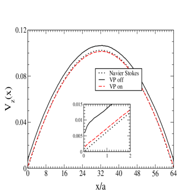
Figure 1: (Colors online) Velocity profile across a slit of width $L_{x}$. Simulations are performed in a box of sides $L_{x}=L_{y}=L_{z}=64a$. The external applied field is $\bm{F}^{ext}=10^{-4}f_{0}\bm{\hat{z}}$. The inset shows a magnification of the profile near the wall at $x=0$.

Simulation results for the case ${\bf{F}}^{ext}=10^{-4}f_{0}\bm{\hat{z}}$, with $f_{0}=k_{B}T/a$ are plotted in Fig. (1). When the no-slip BC are implemented only in the streaming step, using the stochastic reflections according to Eqs. (2-3), the slope of the velocity profile (solid line) just near the wall is different from the expected one (dotted line); moreover large slippage near the wall persists. When VP are included into the collision step, the $v_{z}(x)$ profile (dashed line) reproduces quite well the Navier-Stokes solution. The use of VP clearly ameliorates the simulation results with no-slip BC as expectedLamura et al. (2001); R.G. Winkler and C.C. Huang (2009); I.O. Gotze et al. (2007). We next ask what are the consequences of the various changes for the force exerted by the fluid upon the wall? From a balance of external body and wall forces in a stationary state, the expected value of the force on each wall is $f^{exp}=\gamma F^{ext}\frac{L_{x}}{2}L_{y}L_{z}$ Durst (2008), which in our case is $f^{exp}=16f_{0}$.
In Fig. (2) we see that the total force converges to the expected value of $f^{exp}=16f_{0}$, at which point a stationary state is reached. In the stationary state the contribution to the total force due to the collision step ($\bm{f}_{c}$) is relatively large. This happens especially when the mean free path of the MPCD fluid is small, in which case momentum is transported mainly via collisions rather than via diffusion.

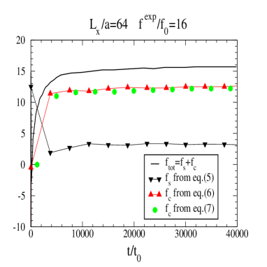
Figure 2: (colors online)Average force exerted by the fluid upon each wall of a slit of width $L_{x}=64a$, versus time. The total expected value is $f^{exp}=16f_{0}$; $f_{s}$ and $f_{c}$ are the force exerted during the streaming and the collision steps.

For the slit geometry it is easy to adapt the general expression for the stress tensor of the MPCD fluid with periodic BC Ihle and Kroll (2001); Ihle and D.M. Kroll (2003) in order to measure the force just near the wall. The force exerted along the $\bm{\hat{z}}$ direction because of collisional exchange of momentum along the $\bm{\hat{x}}$ direction is:

$$f_{c}=\frac{m}{\delta t}\overset{p}{\sum_{j=1}}\Delta\xi_{j,x}^{S}\Delta v_{j,z}.$$ (7)

In this expression we have used the same notation as adopted in Ihle and Kroll (2001), where a full description of the MPCD stress tensor is provided. The meaning of the notation is as follows: $\Delta\xi_{j,x}^{S}=\xi_{j,x}(t+\delta t)-\xi_{j,x}^{S}(t+\delta t)$, $\Delta v_{j,z}=V_{j,z}(t+\delta t)-v_{j,z}(t+\delta t)$; $V_{j,z}$ and $v_{j,z}$ are the $z$ component of the velocities after and before the collision step of particle $j$. $\xi_{j}(t)=(\xi_{j,x},\xi_{j,y},\xi_{j,z})$ are the coordinates of the cell of the unshifted grid containing the particle j at time $t$. Similarly $\xi_{j}^{S}$ are the coordinates of the cell of the shifted grid containing the $j$ particle at time $t$. The sum in Eq. (7) applies only to the $p$ particles of the MPCD solvent belonging to the cells which overlap one of the walls. As shown in Fig. (2), the expressions of the forces according to Eq. (6) and (7) are in very good agreement. However, if one needs the force exerted by the fluid upon a spherical colloid or an irregularly shaped object, it is important to take into account the local curvature of the colloidal surface. In such a case the generalization of the stress tensor for the MPCD fluid is not easy, while the implementation of Eq. (6) is straightforward.

IV Friction on a sphere in the bulk

We now turn to the translational friction on a sphere which is not free to rotate. In this respect we consider the case of a single sphere of radius $R_{col}=4a$, which is kept at a fixed position by applying a constraint force $\bm{\mathcal{F}}^{c}$. This condition is similar to the case of very massive particles embedded in solvent as studied in Whitmer and Luijten (2010). We use a cubic simulation box whose side is $L=32a$. We are primarily interested in the autocorrelation function of $\bm{\mathcal{F}}^{c}$ because this can be connected, via a Green-Kubo relation, to the translational friction tensor R.L.C. Akkermans and W.J. Briels (2000):

$$\Xi_{\alpha\beta}=\lim_{t\rightarrow\infty}\frac{1}{k_{B}T}\int_{0}^{t}d\tau\left\langle\mathcal{F}_{\alpha}^{c}(t_{0}+\tau)\mathcal{F}_{\beta}^{c}(t_{0})\right\rangle_{t_{0}}$$ (8)

where $\alpha,\beta\in\{x,y,z\}$.

Because of symmetry, the friction does not depend on the cartesian direction along which we measure, see Fig. (3).

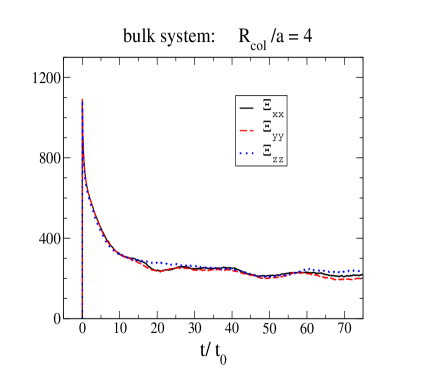
Figure 3: (Colors online) Running integral of the autocorrelation functions of the constraint force. The off-diagonal terms of Eq. (8), which are not shown here, go quickly to zero.

If we consider a particular direction $\alpha$, the long time limit of $\Xi_{\alpha\beta}$ provides the total friction $\xi$ upon the sphere, for which there are essentially two contributions: one coming from the local Brownian collisions with the particles of the fluid ($\xi_{E}$), while the other is due to the long-range hydrodynamic interactions ($\xi_{S}$). A simple empirical formula says that the hydrodynamic and the Brownian friction should be added in parallel J.T. Hynes (1977); S.H. Lee and Kapral (2004) in order to obtain the total friction:

$$1/\xi=1/\xi_{E}+1/\xi_{S}.$$ (9)

Both $\xi$ and $\xi_{E}$ may be calculated using our simulations. $\xi$ can be read from the long-time limit of the integral in Eq.(8),while $\xi_{E}$ corresponds to the height of the short-time peak J.T. Padding and W.J. Briels (2010). The hydrodynamic term can be extracted by inverting Eq.(9). In the present case we obtain $\xi_{E}^{sim}~{}=~{}1088~{}\pm~{}4$ and $\xi_{S}^{sim}~{}=~{}270~{}\pm~{}30$.
The hydrodynamic friction can be theoretically estimated from the drag force $\bm{F}_{d}$ on a colloid with no-slip BC in an infinite fluid medium, according to the Stokes law $\bm{F}_{d}=-\xi_{S}^{\infty}\bm{v}_{\infty}=-6\pi\eta R_{col}\bm{v}_{\infty}$, where $\bm{v}_{\infty}$ is the flow field at large distances. As the Stokes friction depends on the long-range hydrodynamic effects, it can be substantially affected by the finite-size $L$ of the simulation box. Detailed calculations in Dünweg and Kremer (1993) suggest that to lowest order in $R_{col}/L$, the correction is given by $\xi_{S}=\xi_{S}^{\infty}\beta\left(R_{col}/L\right)$, with

$$\beta\left(R_{col}/L\right)\approx\left(1-2.837\left(R_{col}/L\right)\right)^{-1}$$ (10)

Taking into account the finite-size effects, the value for the Stokes friction is $\xi_{S}=291$, and the simulations result is in good agreement with this.

We now turn to the Brownian friction $\xi_{E}$, due to local collisions with the solvent. A suitable starting point to calculate this term is the Enskog-Boltzmann theory for a dense gas. This model takes into account only two-bodies collisions and successive collisions are supposed to be uncorrelated. In other words no influence of the local disturbance, induced by the tagged colloidal particle on its surroundings, is included. The expression for the translational friction in a bath of particles of mass $m$ is the following J.T. Padding et al. (2005):

$$\xi^{\prime}_{E}=\frac{8}{3}\left(\frac{2\pi k_{B}TmM}{m+M}\right)^{1/2}\gamma R_{col}^{2}\frac{1+2\chi}{1+\chi},$$ (11)

where $\chi=I/MR_{col}^{2}=2/5$ is the gyration ratio for a sphere. According to this model $\xi_{E}\sim 700$, while from simulations we obtain a much larger value. The discrepancy is a consequence of the changes made to the collision step, as the exchange of momentum between the MPCD particles and the colloid, via VP, changes the effective number of local Brownian collisions.

In order to evaluate the fluctuations in the constraint force $\bm{\mathcal{F}}^{c}$ due to the VP, let us focus on one collision cell which partly overlaps with a colloid and contains $p$ MPCD particles and $q$ VP, with velocities $\mathbf{v}_{i}$ and $\mathbf{w}_{i}$, respectively. Let us suppose that the colloid moves with velocity $\mathbf{V}$ through the ideal gas bath, then we know that

$$\left\langle\mathbf{v}_{i}\right\rangle=\mathbf{0} \left\langle v_{i}^{2}\right\rangle=\frac{3k_{B}T}{m}$$ (12)

$$\left\langle\mathbf{w}_{i}\right\rangle=\mathbf{V} \left\langle(\mathbf{w}_{i}-\mathbf{V})^{2}\right\rangle=\frac{3k_{B}T}{m}$$ (13)

The collision step itself may be written as (primes indicate velocities after the collision):

$$\bm{u} = \frac{1}{p+q}\left(\sum_{i=1}^{p}\mathbf{v}_{i}+\sum_{i=1}^{q}\mathbf{w}_{i}\right)$$ (14)

$$\mathbf{v}_{i}^{\prime} = \mathbf{v}_{i}+(\bm{\Omega}-\mathbf{I})\left(\mathbf{v}_{i}-\bm{u}\right)$$ (15)

$$\mathbf{w}_{i}^{\prime} = \mathbf{w}_{i}+(\bm{\Omega}-\mathbf{I})\left(\mathbf{w}_{i}-\bm{u}\right)$$ (16)

where $\bm{\Omega}$ represents a rotation of an angle $\alpha$ around a random axis, $\mathbf{I}$ is the unit matrix, and $\bm{u}$ the average velocity of the cell center of mass. The total change of momentum of the VP, i.e. their contribution to the change of momentum of the colloid (or wall) is equal to:

$$\Delta\mathbf{P}^{VP} = m\sum_{i}^{q}\left(\mathbf{w}_{i}^{\prime}-\mathbf{w}_{i}\right)$$

$$= m(\bm{\Omega}-\mathbf{I})\left[\frac{p}{p+q}\sum_{i}^{q}\mathbf{w}_{i}-\frac{q}{p+q}\sum_{i}^{p}\mathbf{v}_{i}\right].$$

We define the force exerted on the colloid by the cell under consideration as $\bm{F}^{VP}=\Delta\bm{P}^{VP}\delta t$ and consider its contribution to the Enskog friction matrix:

$$\bm{\Xi}(t) = \beta\int_{0}^{t}\left\langle\mathbf{F}(\tau)\mathbf{F}(0)\right\rangle\mathrm{d}\tau$$

$$= \frac{1}{2}\beta\left\langle\mathbf{F}(0)\mathbf{F}(0)\right\rangle\delta t+\sum_{j=1}^{i}\left\langle\mathbf{F}(j\delta t)\mathbf{F}(0)\right\rangle\delta t.$$

Only the first term will be non-zero because velocities at different times are uncorrelated. When calculating this term, we assume $<\bm{v}_{i}\bm{v}_{j}>=\frac{k_{B}T}{m}\mathbf{I}\delta_{i,j}$, $<\bm{w}_{i}\bm{w}_{j}>=\frac{k_{B}T}{m}\mathbf{I}\delta_{i,j}$ and $<\bm{v}_{i}\bm{w}_{j}>=0$, which turns $\bm{\Xi}=\bm{\Xi}(0)$ into a diagonal matrix. Averaging over all possible orientations of the rotation axis we obtain for the diagonal elements:

$$\xi_{VP}=\frac{2}{3}(1-\cos\alpha)\frac{m}{\delta t}\frac{pq}{p+q}.$$ (19)

Since velocities in different cells are uncorrelated we may simply add the contributions of all cells overlapping with the colloid, obtaining:

$$\xi_{VP}^{tot}=\frac{2}{3}(1-\cos\alpha)\frac{m}{\delta t_{c}}\sum_{\mathrm{cells}\ k}\frac{p_{k}q_{k}}{p_{k}+q_{k}}.$$ (20)

Performing the sum over cells analytically is rather complicated, if not impossible, so we have decided to evaluate Eq. (20) numerically, during the simulation itself. Including the correction so obtained, the predicted short time friction becomes: $\xi_{E}~{}=~{}\xi^{\prime}_{E}~{}+~{}\xi_{VP}^{tot}~{}=~{}1084$, which is in very good agreement with the simulation value $\xi_{E}^{sim}~{}=~{}1088~{}\pm~{}4$.

V Friction on a sphere inside a slit

Recent developments in the field of micro- and nanofluidics have led to a renewed interest in molecular hydrodynamics phenomena near a solid surface. It has been shown theoretically Ganatos et al. (1980); Happel and Brenner (1991); Cichocki and R.B. Jones (1998); Bhattacharya et al. (2005) and experimentally Malysa and T.G.M. van de Ven (1986); Lobry and Ostrowsky (1996); Lin et al. (2000); Leach et al. (2009) that the hydrodynamic interactions with flat walls can slow down the motion of colloidal particles substantially, and that such effect also depends on the direction of the motion of the particle (for example parallel or perpendicular to the walls). We therefore apply our method to study the friction on a sphere inside a slit. In this case, as in the bulk system, we do not take into account the role played by the angular momentum, so that the present discussion is relevant only for purely translating spheres in a slit. The walls are set at $z=0$ and $z=L_{z}$ while we use periodic BC along the $x$ and $y$ directions.The length of the walls’ sides is $L_{x}=L_{y}=L$. We have chosen this particular configuration because we have access to analytical solutions of the Navier-Stokes equations for the parallel motion Happel and Brenner (1991) and numerical solutions for the perpendicular motion as well Bhattacharya et al. (2005). Such solutions have been provided under the assumption that the lateral size ($L$) of the walls is infinitely large.

Our aim is to study how the friction depends on the lateral width $L$ of the cell when the walls separation $L_{z}$ is fixed. Besides establishing finite size effects for the usual simulation boxes, this topic is also relevant for the study of experimental periodic arrangements of particles, such as trains and grids of particles under confinement. In both cases a periodic array of colloidal particles exists, exerting strong hydrodynamic interactions on each other.
Simulations have been performed keeping the colloidal particle of Sec.IV in a fixed position in the mid-plane of the slit. From the autocorrelation of the constraint force we obtain the friction coefficients (as explained in section IV) in the directions parallel and perpendicular to the walls. Under the assumption of small Reynolds numbers, it is possible to express the effects of the walls by means of a correction factor $\tau$ to the Stokes friction $\xi_{S}^{\infty}$ in an unbounded system:

$$\xi^{\perp}_{1}=\tau^{\perp}\xi_{S}^{\infty}.$$ (21)

Similarly we describe finite-size effects by a second correction factor $\beta$:

$$\xi^{\perp}_{2}=\beta^{\perp}\tau^{\perp}\xi_{S}^{\infty}.$$ (22)

In the following we will obtain $\beta^{\perp}$ as

$$\beta^{\perp}=\xi^{\perp}_{sim}/\xi_{1}^{\perp}.$$ (23)

Similar expressions hold for the parallel frictions.

Analytical expressions for the parallel and perpendicular frictions in a slit geometry are not available, but analytical expression for a single wall do exist Happel and Brenner (1991). The correction for the parallel friction due to the presence of a single wall is:

$$\tau^{||} = \left[1-1.004(R_{col}/z)+0.418(R_{col}/z)^{3}+\right.$$ (24)

$$\left.+0.21(R_{col}/z)^{4}-0.169(R_{col}/z)^{5}\right]^{-1},$$

whereas the correction for the perpendicular friction is:

$$\tau^{\perp} = \frac{4}{3}\sinh(\alpha)\sum_{{}_{n}=1}^{\infty}\frac{n(n+1}{(2n-1)(2n+3)}\times$$

$$\left(\frac{2\sinh(2n+1)\alpha+(2n+1)\sinh 2\alpha}{4\sinh^{2}(n+0.5)\alpha-(2n+1)^{2}\sinh^{2}(\alpha)}-1\right),$$

where $\alpha=\cosh^{-1}\left(z/R_{col}\right)$ and $z$ is the distance of the particle from the wall. As a first approximation, we use linear superposition theory, according to which we can add the contributions coming from each wall as if they behave independently from one another:

$$\tau_{\infty}^{\perp}\approx\tau^{\perp}_{w1}+\tau^{\perp}_{w2}-1,$$ (26)

the subscripts $w1$ and $w2$ refer to the two walls. We have subtracted 1, in order to avoid counting the bulk contribution to the friction twice. This is a mere consequence of the definition adopted for the corrective terms.

In case the walls are very far apart, this approximation works fairly well, otherwise it tends to overestimate the combined effects of the two walls. In particular, for the simulation parameters we have used here ($R_{col}=4a$ and $L_{z}=32a$), the friction obtained with the superposition model appears to be overestimated by about $15\%$ with respect to the numerical solution of the Navier-Stokes equations in the slit as given in Bhattacharya et al. (2005). In the rest of this section we will use the results provided by Eq.(26) but corrected according to Bhattacharya et al. (2005).

The values of $\beta^{\perp,||}$ are plotted in Fig. (4) as a function of lateral size $L$.

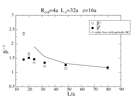
Figure 4: Finite-size effects corrections for the friction upon a spherical particle placed in the mid-plane of a slit geometry. The lateral size of the square walls is $L$, while the wall separation is $L_{z}=32a$. Circles: simulation results. Solid line: the corrective terms for a cubic box with periodic BC in all three directions (Eq.10).

For values of $L<24a$, the behavior of $\beta^{||}$ and $\beta^{\perp}$ is very different: with decreasing $L$, $\beta^{||}$ decreases while $\beta^{\perp}$ increases. For the parallel motion we expect that, when the lateral size $L$ is very small and the particle is very close to its images, a wake effect is established which reduces the friction along the lines connecting the colloid and its nearest images. A similar trend can be deduced from Bhattacharya (2008); S.C. Hohale and Khare (2008). The situation depicted in these works is slightly different from ours. They for example study the parallel friction as a function of $L_{x}$ once $L_{y}$ and $L_{z}$ are fixed, while in the present simulations we always use a square periodic space ($L_{x}=L_{y}$). However if, for each profile shown in Bhattacharya (2008); S.C. Hohale and Khare (2008), we pick up the points corresponding to $L_{x}=L_{y}$, it is seen that the friction decreases as $L$ diminishes. On the contrary when $L>24a$, the parallel and perpendicular frictions behave similarly: they decay slowly to the case of a slit whose walls are infinitely large. It is possible that the screening point where we can observe different behaviors between the parallel and perpendicular friction is for $L\sim L_{z}$.

When $L=L_{z}$, the simulation box is cubic, so we can compare our results with those provided by the correction factors in Eq. (10) plotted in Fig. (4) as a solid line. We see that there exists a significant difference which is due just to the presence of the confining walls: the latter screen even the effects due to the use of periodic BC. However, once the wall separation $L_{z}$ is fixed, the correction factor decays slower when compared to Eq. (10) where periodic BC are used in all directions (Fig. (4)).

For ease of use, we have tried to fit the data for $L>20$ with a function similar to that in Eq. (10) (see red lines in Fig. (5)): the behavior seems good for the perpendicular friction but it deteriorates for the parallel friction.

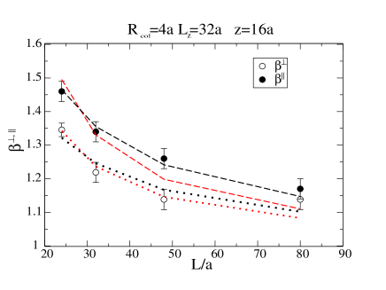
Figure 5: (Colors online) Finite-size effects for $L>20$ in comparison with two different fit functions. Red lines are based on a function of the type as in Eq. (10); black lines are based upon the function in Eq. (27). Dotted lines are for the perpendicular friction, dashed lines for the parallel one.

We have also tried a fit with the function

$$f(L)=1+A\ln(1+R_{col}/L),$$ (27)

in which $A$ is a parameter whose value depends on the direction we consider: for the parallel friction $A^{||}~{}\sim~{}2.08$ while for the perpendicular motion $A^{\perp}~{}\sim 3.02$. Eq. (27) seems to work better than Eq. (10). For example the parallel friction is better captured (see black lines in Fig. (5)). We do not have, however, indications whether the parameter $A$ is a function of the wall separation $L_{z}$ and of the particle position $z$. To clarify this point further simulations are necessary, to be compared with the solutions of the Navier-Stokes equations for the slit for different particle positions.

In summary, our results suggest that:

• There are two different regimes depending on whether the lateral size of the walls is smaller or larger than the wall separation.

• For a cubic box, the finite size effects in the slit geometry are less than in a system with periodic BC in all three directions.

• Once $L_{z}$ is fixed and $L>L_{z}$, the correction factors $\beta^{\perp,||}$ decay slowly towards unity, possibly as a logarithmic function of $L$.

VI Conclusions

In conclusion we have described a protocol for the MPCD simulation technique, which provides a satisfactory treatment of the no-slip boundary conditions (BC) and the correct evaluation of the force exerted by the solvent on solid surfaces. Such a protocol is based upon the use of virtual particles during the collision-step, a method already used in literature and which appears suited to study wall-liquid interfaces and very massive particles embedded in the solvent, or particles kept fixed by an external constraint force as in the present work. We pay particular attention to the calculation of the friction tensor for a non rotating sphere.
We have shown how the no-slip BC modifies the local Brownian friction on a spherical colloid, and how such effects can be evaluated through an Enskog-like treatment of the VP. We have also studied the friction on a particle embedded in a slit, analyzing the dependence of the simulation results on the use of periodic boundary conditions along the sides of the walls. When the lateral size of the walls is very small (less than the wall separation), strong coupling effects between a particle and its images are observed. Moreover, the parallel and the perpendicular friction show an antithetic behavior: as $L$ decreases, the parallel friction decreases too, while the perpendicular friction increases. When $L>L_{z}$, the corrective terms for the parallel and perpendicular friction are much more similar to each other and they both decrease to unity as $L$ increases, approaching more and more the case of an ideal slit made of two infinitely large walls. When $L=L_{z}$, we find that the finite-size effects (FSE) in the slit geometry are less than for a cubic box with periodic boundary conditions in all directions. Moreover, once $L_{z}$ is fixed and $L>L_{z}$, the FSE in the slit appear to be slowly varying with the system size $L$, possibly according to a logarithmic function of $R_{col}/L$.
Further studies will concern whether and how the FSE in a slit depend on the walls’ separation $L_{z}$ and on the particle distance $z$.

References

- Malevanets and Kapral (1999) A. Malevanets and R. Kapral, J. Chem. Phys. 110, 865 (1999).
- Gompper and et al. (2009) G. Gompper and et al., Adv. Polym. Sci. 221, 1 (2009).
- Boquet and J.L. Barrat (1994) L. Boquet and J.L. Barrat, PRE 49, 3079 (1994).
- Lauga et al. (2005) E. Lauga, M.P. Brenner, and H. Stone, Handbook of experimental fluid dynamics (J. Foss and C. Tropea and A. Yarin (New York: Springer), 2005).
- Lamura et al. (2001) A. Lamura, G. Gompper, T. Ihle, and D.M. Kroll, Europhysics Letters 56, 319 (2001).
- R.G. Winkler and C.C. Huang (2009) R.G. Winkler and C.C. Huang, J. Chem. Phys 130, 074907 (2009).
- I.O. Gotze et al. (2007) I.O. Gotze, H. Noguchi, and G. Gompper, PRE 76, 046705 (2007).
- M.T. Downton and Stark (2009) M.T. Downton and H. Stark, J. Phys.: Condes. Matter 21, 204101 (2009).
- Whitmer and Luijten (2010) J. Whitmer and E. Luijten, J.Phys.:Condes.Matter 22, 104106 (2010).
- Dünweg and Kremer (1993) B. Dünweg and K. Kremer, J. Chem. Phys. 99, 6983 (1993).
- Zick and Homsy (1982) A. Zick and G. Homsy, J. Fluid Mech. 115, 13 (1982).
- S.C. Hohale and Khare (2008) S.C. Hohale and R. Khare, J. Chem. Phys. 129, 164706 (2008).
- Bhattacharya (2008) S. Bhattacharya, J. Chem. Physics 128, 074709 (2008).
- Malevanets and Kapral (2000) A. Malevanets and R. Kapral, J. Chem. Phys. 112, 7260 (2000).
- Ihle and Kroll (2001) T. Ihle and D. Kroll, Phys. Rev. E 63, 020201(R) (2001).
- J.T. Padding and A.A. Louis (2006) J.T. Padding and A.A. Louis, Phys. Rev. E 74, 031402 (2006).
- Durst (2008) F. Durst, Fluid Mechanics:An introduction to the theory of fluid flows (Springer, 2008).
- Ihle and D.M. Kroll (2003) T. Ihle and D.M. Kroll, Phys. Rev. E p. 066706 (2003).
- R.L.C. Akkermans and W.J. Briels (2000) R.L.C. Akkermans and W.J. Briels, J. Chem. Phys. 132, 054511 (2000).
- J.T. Hynes (1977) J.T. Hynes, Annu.Rev.Phys.Chem. 28, 301 (1977).
- S.H. Lee and Kapral (2004) S.H. Lee and R. Kapral, J. Chem. Phys. 121, 11163 (2004).
- J.T. Padding and W.J. Briels (2010) J.T. Padding and W.J. Briels, J. Chem. Phys. 132, 054511 (2010).
- J.T. Padding et al. (2005) J.T. Padding, A. Wysocki, H. Lowen, and A.A. Louis, J. Phys.: Condensed Matter 17, S3393 (2005).
- Ganatos et al. (1980) P. Ganatos, S. Weinbaum, and R. Pfeffer, J. Fluid Mech. 99, 739 (1980).
- Happel and Brenner (1991) J. Happel and H. Brenner, Low Reynolds Number Hydrodynamics (Lluwer, 1991), 5th edition.
- Cichocki and R.B. Jones (1998) B. Cichocki and R.B. Jones, Physica A 258, 273 (1998).
- Bhattacharya et al. (2005) S. Bhattacharya, J. Blawzdziewicz, and E. Wajnryb, Physica A 356, 294 (2005).
- Malysa and T.G.M. van de Ven (1986) K. Malysa and T.G.M. van de Ven, Int. J. Multiphase Flow 12, 459 (1986).
- Lobry and Ostrowsky (1996) L. Lobry and N. Ostrowsky, PRE 53, 12050 (1996).
- Lin et al. (2000) B. Lin, J. Yu, and S.A. Rice, PRE 62, 3909 (2000).
- Leach et al. (2009) J. Leach, H. Mushfique, S. Keen, R. Di Leonardo, G. Ruocco, and M.J. Padgett, PRE 79, 026301 (2009).