Slow relaxation and aging kinetics for the driven lattice gas

Abstract

We numerically investigate the long-time behavior of the density-density auto-correlation function in driven lattice gases with particle exclusion and periodic boundary conditions in one, two, and three dimensions using precise Monte Carlo simulations. In the one-dimensional asymmetric exclusion process on a ring with half the lattice sites occupied, we find that correlations induce extremely slow relaxation to the asymptotic power law decay. We compare the crossover functions obtained from our simulations with various analytic results in the literature, and analyze the characteristic oscillations that occur in finite systems away from half-filling. As expected, in three dimensions correlations are weak and consequently the mean-field description is adequate. We also investigate the relaxation towards the nonequilibrium steady state in the two-time density-density auto-correlations, starting from strongly correlated initial conditions. We obtain simple aging scaling behavior in one, two, and three dimensions, with the expected power laws.

I Introduction

Driven lattice gases represent perhaps the simplest models of interacting non-equilibrium systems that nevertheless display intriguingly complex features, and consequently have been carefully studied for many years now beatebook ; hh_rev ; derr1 ; guntbook ; kirone_rev . Since there exists to date no general theoretical framework to adequately capture and classify the macroscopic properties of non-equilibrium systems, simple paradigmatic models such as driven lattice gases have proven useful to gain a thorough understanding of at least certain models driven towards out-of-equilibrium stationary states, characterized by non-vanishing macroscopic (probability, particle, or energy) currents.

Let us briefly review the basic features of driven lattice gases with particle exclusion to provide a proper context for the present investigation. For the one-dimensional driven lattice gas with periodic boundary conditions, equal-time correlations have long been established to be trivial and governed by a simple product measure derr1 . Its temporal evolution, in contrast, displays rich features, and is not easily accessible analytically. The Bethe ansatz method was used to calculate the spectral gap at half filling which gives the value of the dynamic exponent dhar ; bethe_1 ; bethe_2 ; spec_osc3 . This approach was later generalized for arbitrary densities spec_osc2 ; spec_osc1 . The Bethe ansatz also allows for calculation of conditional time-dependent probabilities for the lattice gas exact1 ; exact2 . Yet time-dependent correlation functions have only been amenable to very limited general exact solutions most of which are tractable only for very small system sizes. The correlation functions are governed by non-trivial scaling laws even in the stationary state derr1 .

It is well-understood that the large-scale behavior of the driven lattice gas in one dimension is governed in the coarse-grained continuum limit by the noisy Burgers equation Forster , and is also mappable to a surface growth model that belongs to the KPZ universality class kpz . The scaling form of the density-density correlation of the driven lattice gas has been derived and the associated scaling exponents calculated by means of renormalization group techniques Forster ; Jan ; kpz . Scaling functions have been computed by means of the mode-coupling approximation mc_4 ; mc_2 ; uwehwa ; mc_5 ; cola2 ; mc_1 ; mc_3 , exact numerical integration cola ; spohnlong ; schwartz_1 , and other analytical approaches rg_2 ; rg_1 ; fog_1 ; scaling_exact_1 .

In this work, we employ extensive large-scale Monte Carlo simulations to confirm the exactly known scaling exponents in one, two, and three dimensions. We will also compare our numerical data to different predictions for the scaling functions. In one dimension in particular, our Monte Carlo simulations yield a remarkably slow approach to the asymptotic scaling behavior, governed by an unusual form of the associated scaling function. Non-stationary properties of the driven lattice gas in the physical aging regime are considerably less understood. For KPZ surface growth, a renormalization group analysis demonstrated that the so-called initial slip exponent can be related to the dynamical exponent, and no additional singularities associated with the initial-time surface emerge krech . We find that similar scaling relations hold for driven lattice gases in arbitrary dimensions. In addition, for appropriate highly correlated initial conditions (that in the growth model mapping correspond to a flat surface), we establish simple aging scaling in the non-stationary time regime pleimbook . This is in accord with studies that showed simple aging as well for both the KPZ surface growth model krug ; A4 ; michelnew ; yenglobal and its linear counterpart, the Edwards–Wilkinson model A1 ; A3 ; A2 ; yenglobal . A few exact results were found in the non-stationary regime, for small systems sas_lett ; sas_fluc ; time_dep ; sas_pape .

The outline of this paper is as follows. In the following section we describe the models under investigation, comment on our Monte Carlo simulation specifics, define the relevant observables, and provide the dynamic scaling forms for the density-density (and height-height) correlation function. In section III, we present our simulation results in the non-equilbrium steady state for the model, focusing on the behavior in one dimension. Short time results for densities away from half filling yield charactaristic oscillations in the density-density correlation function. Next finite-size scaling features are discussed in some detail. We generate the scaling functions from our simulation data and compare them to the accepted forms. The unusually slow relaxation of the local exponent of the density-density correlation function towards its asymptotic universal value is carefully investigated for the one-dimensional case, and contrasted with the much more straightforward behavior seen in higher dimensions. We conclude this section with a discussion of the effects of finite rather than infinite hopping bias. Section IV contains our simulation results for non-stationary properties of the driven lattice gas, starting from a correlated initial state, in one, two and three dimensions. We cast our results in the standard simple aging scaling form and compute the aging exponents by means of a simple scaling argument, which is a-posteriori confirmed by our simulations.

II The driven lattice gas with exclusion

II.1 Model description

We study driven lattice gases with site exclusion on a $d$-dimensional square lattice of size $L^{d}$ with periodic boundary conditions, with a total number of $N$ particles beatebook ; derr1 ; guntbook . The exclusion constraint limits the site occupation number at a position $x$ on the lattice to the values $n(x)\in\{0,1\}$. The particles may hop to nearest-neighbor lattice sites only if these are empty. In one dimension, this model is referred to as the periodic asymmetric simple exclusion process (ASEP). We denote the probabilities of hopping “forward” and “backward” as $p$ and $q=1-p$, respectively. For $p=q$, no net particle current arises; the system is then in equilibrium. For $p=1$ and hence $q=0$, only unidirectional motion (to the right) is possible, and the model reduces to the totally asymmetric simple exclusion process (TASEP). The generalization of the driven lattice gas model to higher dimensions $d$ is straightforward. After a single specific drive direction is selected, we define the hopping probabilities (to empty sites) along this direction to be $p_{\parallel}$ and $q_{\parallel}=1-p_{\parallel}$, while there is no hopping bias in the $d-1$ transverse dimensions, $p_{\perp}=q_{\perp}$ (symmetric exclusion process, SEP).

In one dimension, this lattice gas model can be mapped to a surface growth problem in the KPZ universality class kpz . To this end, one defines local Ising spin variables $\sigma(x)=1-2n(x)$, where $n(x)$ is the occupation number. The height variable at site $x$ is then given by the accumulated magnetization from the (arbitrary) reference point at site $1$ up to $x$:

$$h(x)=\displaystyle\sum_{y=1}^{x}\sigma(y)=x-2\displaystyle\sum_{y=1}^{x}n(y).$$ (1)

Particle exclusion restricts the local slope of the surface height profile to $\pm 1$. This mapping allows us to directly relate observables such as correlation functions calculated for the surface growth model to those for our driven lattice gas model.

II.2 Monte Carlo simulations

We employ both standard Metropolis and continuous-time Monte Carlo algorithms to study the driven lattice gas. The standard Monte Carlo algorithm New starts with all particles placed at random positions. A particle is randomly selected, and then one of the $2d$ directions for a potential nearest-neighbor hop is randomly chosen. A hop has a predetermined probability $R_{i}\in[0,1]$ ($i=1,\ldots,2d$, $R_{i}$ is either $p_{\parallel}$, $q_{\parallel}$, $p_{\perp}$, or $q_{\perp}$). A random number $r\in[0,1]$ is picked; if $r<R_{i}$ then hop $i$ is performed. Particle exclusion is realized in this simulation by setting $R_{i}=0$ for any hop that attempts to move a particle into an occupied site. One Monte Carlo time step has passed once $N$ hopping attempts have been made. On average the algorithm thus attempts to hop each particle once per Monte Carlo time step. In dimensions $d\geq 2$, the hopping probabilities are asymmetric parallel to the drive (if not mentioned otherwise we use $p_{\parallel}=1$, $q_{\parallel}=0$), and symmetric in the transverse directions $p_{\perp}=q_{\perp}=1/2$. With the periodic boundary conditions, this prescription generates a (fluctuating) particle current along the drive direction.

For the one-dimensional system we employ the continuous-time Monte Carlo algorithm Borz ; New , which is initialized the same way as the standard Monte Carlo process. The crucial feature of this algorithm is that hops are never rejected; they are simply performed at the correct rates. The probability for each possible hop $i$ from a given configuration $C$ of the system is $R_{i}$. An active list is kept of all possible hops with $R_{i}\not=0$, and the next hop is chosen by sampling the list. Time is incremented by $\Delta t=1/\sum_{i}R_{i}$. For the driven lattice gas with exclusion, each site has an equal probability of being occupied, equal to the filling fraction or mean density $\rho=N/L$; e.g., for a half-filled system the probability is $\rho=1/2$. This algorithm eliminates all attempted hops that would be rejected due to exclusion. This is realized in the simulation as follows for the ASEP. Two lists are maintained, $L_{r}$, $L_{l}$, one for the hops to the right and left with probabilities $p$ and $q$, normalized by $p+q=1$. A random number $r\in[0,1]$ is generated. If $r<p$, a hop to the right is performed, if $r>p$ we chose a hop to the left. Note that we may only proceed in this manner because the list lengths $N_{h}$ of possible left and right hops are equal. A random integer $n\in[1,N_{h}]$ is selected, and we correspondingly update the $n$th particle in the $L_{r}$ or $L_{l}$ list. The time counter is increased by $\Delta t$ which is calculated using the rates prior to the hop being performed. This continuous-time algorithm yields an efficiency enhancement of approximately a factor of $2$, because only hops which can be performed are chosen, and consequently allows us to increase the effective simulation time by that factor also. We note that in the following, all distances and times will be measured in units of the lattice spacing and Monte Carlo Steps (MCS), respectively.

II.3 Quantities of interest

Our starting point is the two-time density-density (connected) correlation function (cumulant), defined as

$$S(\vec{x}^{\prime},\vec{x},t^{\prime},t)=\langle n(\vec{x},t)n(\vec{x}^{\prime},t^{\prime})\rangle-\langle n(\vec{x}^{\prime},t^{\prime})\rangle\langle n(\vec{x},t)\rangle,$$ (2)

where $\langle\cdot\rangle$ denotes an ensemble average over (many) stochastic realizations. In the stationary state, a periodic system becomes translationally invariant in both space and time. Therefore the correlation function depends only on coordinate and time differences. Defining the average density $\rho=\langle n(\vec{x},t)\rangle=N/L$, we then obtain

$$S(\vec{x}^{\prime}-\vec{x},t^{\prime}-t)=\langle n(\vec{x},t)n(\vec{x}^{\prime},t^{\prime})\rangle-\rho^{2}.$$ (3)

For the driven lattice gas (ASEP) in the stationary state, it is well known that each possible particle configuration $C$ occurs with equal probability $P^{*}(C)$, namely the inverse of the number $N(C)={L\choose N}$ of possible states

$$P^{*}(C)=\frac{1}{N(C)}=\frac{N!(L-N)!}{L!}\ .$$ (4)

This independent-particle result remarkably remains valid even in the presence of on-site particle exclusion meak . However, if nearest-neighbor interactions were added, the stationary probabilities would depend on the particles’ relative positions.

¿From the simple product measure (4), we can readily obtain the equal-time stationary density-density correlation function $S(\vec{x}^{\prime}-\vec{x}\not=0,t^{\prime}-t=0)$. The probability to find a particle at a given site $\vec{x}$ is just the average density $\rho=N/L$, and given that site $\vec{x}$ is occupied the density at a different site $\vec{x}^{\prime}\not=\vec{x}$ is $(N-1)/(L-1)$, which yields $\langle n(\vec{x},t)n(\vec{x}^{\prime},t)\rangle=\sum_{C}P^{*}(C)n(\vec{x})n(\vec{x}^{\prime})=\sum_{C^{\prime}}P^{*}(C^{\prime})N(N-1)/L(L-1)$. The sum now extends over configurations $C^{\prime}$, which encompass all possible states of $N-2$ particles in the remaining $L-2$ sites, whose stationary probability $P^{*}(C^{\prime})$ is again given by Eq. (4). But the summation gives us a multiplicative factor $N(C^{\prime})=1/P^{*}(C^{\prime})$, which is the number of possible configurations of the remaining $N-2$ particles placed in the remaining $L-2$ sites. Hence we arrive at the simple result $\langle n(\vec{x},t)n(\vec{x}^{\prime},t)\rangle=N(N-1)/L(L-1)$, and the equal-time correlation function becomes

$$S(\vec{x}^{\prime}-\vec{x}\not=0,0)=\frac{N}{L}\frac{N-1}{L-1}-\left(\frac{N}{L}\right)^{2}.$$ (5)

Taking the thermodynamic limit $N,L\to\infty$ while keeping $\rho=N/L$ constant, the correlation function (5) vanishes for $\vec{x}\not=\vec{x}^{\prime}$. However, in a finite system, Eq. (5) yields a negative value

$$S_{\rm min}=\rho\frac{(\rho L-1)}{L-1}-\rho^{2}=-\frac{\rho(1-\rho)}{L-1},$$ (6)

reflecting the particle anti-correlations induced by site exclusion.

A more interesting quantity to study is the two-time (connected) auto-correlation function $S(\vec{x},\vec{x},t^{\prime},t)$, which in the stationary state can be written as $S(0,t)=\langle n(\vec{x},0)n(\vec{x},t)\rangle-\rho^{2}$.

In a finite one-dimensional system with periodic boundary conditions, i.e., a ring with $L$ sites, another notable quantity is the velocity of a single “tagged” particle derr1

$$v_{t}=\frac{L-N}{L-1}\ .$$ (7)

We have checked and confirmed this tagged particle velocity in our Monte Carlo simulations. Note that $v_{t}=1-\rho$ in the thermodynamic limit. Since our numerical data are obtained in finite systems, the typical return time $t_{r}=L/v_{t}$ for a specific particle to traverse the entire ring and come back to its original site posits an upper limit to the argument $t<t_{r}$ for a meaningful analysis of the time-dependent auto-correlation function $S(0,t)$. We remark that the tagged particle velocity has to be carefully distinguished from the propagation speed of a collective density fluctuation guntbook

$$v_{c}=1-2\rho,$$ (8)

which vanishes only at half-filling $\rho=1/2$.

II.4 Dynamic scaling

In the scaling limit, the steady-state density-density correlations for the driven lattice gas with exclusion in $d$ dimensions are described by a general homogeneous function of the following form beatebook

$$S(\vec{x}_{\perp},x_{\parallel},t)=b^{d+\Delta}S\Bigl{(}b\vec{x}_{\perp},b^{1+\Delta}x_{\parallel},b^{z}t\Bigr{)},$$ (9)

where $b$ represents an arbitrary real scale factor, and the subscripts $\perp$ and $\parallel$ denote transverse and parallel directions with respect to the drive. The exponents $\Delta$ and $z$ are the anisotropy and (transverse) dynamical exponents, respectively. A renormalization group analysis Jan yields the upper critical dimension $d_{c}=2$, and the exact exponent values $z=2$ and $\Delta=(2-d)/3$ for $d<d_{c}$. For $d>d_{c}$ the exponents are given by mean-field theory, i.e., $z=2$ and $\Delta=0$, with logarithmic corrections at $d_{c}=2$. Setting $b=t^{-1/z}$, Eq. (9) becomes

$$S(\vec{x}_{\perp},x_{\parallel},t)=t^{-(d+\Delta)/z}f_{d}\Bigl{(}t^{-1/z}\vec{x}_{\perp},t^{-1/z_{\parallel}}x_{\parallel}\Bigr{)},$$ (10)

where $z_{\parallel}=z/(1+\Delta)$ is the dynamical exponent along the drive direction. Taking $\vec{x}_{\perp},x_{\parallel}\to 0$, we obtain for the density auto-correlation function in the scaling limit:

$$S(0,0,t)\sim t^{-\zeta},\ \zeta=\frac{d+\Delta}{z}=\frac{d+\Delta}{(1+\Delta)z_{\parallel}}\ .$$ (11)

In order to carefully characterize the approach to the asymptotic regime in our Monte Carlo simulations, we shall utilize a corresponding local (effective) exponent defined via

$$-\zeta_{\rm eff}(t)=\frac{\log S(0,t)-\log S(0,t-1)}{\log t-\log(t-1)}\ .$$ (12)

A more detailed discussion of each dimension is in order at this point:

$d=1$. The transverse spatial directions become obsolete, and with the exact renormalization group result $\Delta=1/3$ we obtain $z_{\parallel}=3/2$ and $\zeta=1/z_{\parallel}=2/3$. As mentioned above, the scaling behavior for the equivalent surface growth model falls into the KPZ universality class kpz . The central quantity in this description is the height-height correlation function

$$C(x,t)=\Big{\langle}[h(x,t)-h(0,0)]^{2}\Big{\rangle},$$ (13)

which is related to the density-density correlation function via spohn_proc

$$S(x,t)=\frac{1}{8}\frac{\partial^{2}}{\partial x^{2}}C(x,t).$$ (14)

Asymptotically, it takes the scaling form

$$C(x,t)=b^{-2\alpha}C(bx,b^{z_{\parallel}}t),$$ (15)

with the roughness exponent $\alpha$ (note that in the growth model literature, the dynamical exponent $z_{\parallel}$ is usually labeled $z$). According to Eqs. (14) and (15), we can therefore identify $2-2\alpha=(d+\Delta)z_{\parallel}/z=1$ in one dimension, or $\alpha=1/2=2-z_{\parallel}$ Forster ; kpz ; Jan .

$d=d_{c}=2$. At the upper critical dimension, logarithmic corrections arise. The simple power law (11) is replaced with Forster ; Jan

$$S(0,0,t)\sim\frac{1}{t(\log t)^{1/2}}\ .$$ (16)

Accordingly, in order to capture the approach to the asymptotic scaling limit we need to redefine the local exponent in this case as

$$S(0,0,t)(\log t)^{1/2}\propto t^{-\zeta_{\rm eff}(t)}.$$ (17)

It turns out though that the mean-field approximation

$$S_{\rm MF}(0,0,t)\sim t^{-1}$$ (18)

provides reasonable agreement with our simuation data as well.

$d>2$. Above the critical dimension, the mean-field predictions for the scaling exponents $\Delta=0$ and $z=2=z_{\parallel}$, $\zeta=d/2$ should provide an adequate description of the density auto-correlation function data.

Finally, we address the two-time density auto-correlation function $S(0,t,s)$ in the non-stationary regime when the system relaxes from a strongly correlated initial state that considerably differs from any non-equilibrium steady-state configuration. As we shall explain in more detail in Sec. IV.B below, one expects that the physical aging scaling regime $s\ll t$ is governed by the simple aging scaling form pleimbook

$$S(0,t,s)=s^{-\zeta}h_{S}(t/s).$$ (19)

Indeed, we shall see that this scaling ansatz yields satisfactory data collapse. We remark that in the literature on glassy systems, an alternate so-called subaging fitting, $S(0,t,s)=h_{S}(t/s^{\mu}$) with $\mu<1$, has been popular pleimbook .

III Steady-state results

III.1 Recurrence oscillations in small systems

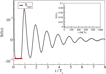
Figure 1: (Color online.) Characteristic recurrence oscillations in the density auto-correlation function $S(0,t)$ for a one-dimensional driven lattice gas (TASEP) at low density $\rho=0.1$ and $L=100$ (close-up). The horizontal (red) line indicates the minimum value $S_{\rm min}=-0.909\times 10^{-3}$ (red line), see Eq. (6). The inset has been included to show the actual magnitude of the oscillations. The return time is $T_{c}=125$ MCS. The data are averaged over 8,000,000 realizations.

We begin with a discussion of small-scale properties of the driven lattice gas on a one-dimensional ring of length $L$ (TASEP). When the total density $\rho=N/L\not=1/2$, collective density fluctuations travel around the system with mean velocity $v_{c}=1-2\rho$. This causes characteristic oscillations in the time-dependent density auto-correlation function $S(0,t)$, with peaks at multiples of the return time $T_{c}=L/v_{c}$, as can be seen clearly in Figs. 1 and 2, which show data obtained for $L=100$ and $L=2000$, respectively, both at low density $\rho=0.1$. (We only report results for densities less than $1/2$, since as a consequence of particle-hole symmetry, the results for $\rho=0.5-\delta$ are equivalent to those for $\rho=0.5+\delta$.)

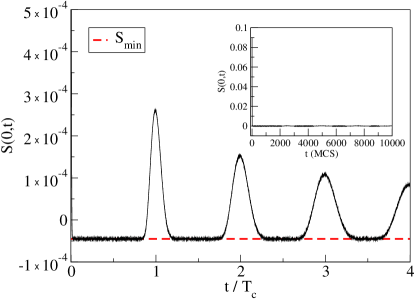
Figure 2: (Color online.) Recurrence oscillations in the driven lattice gas (TASEP) auto-correlation function $S(0,t)$, again for $\rho=0.1$, but a larger one-dimensional ring of length $L=2000$; here $S_{\rm min}=0.45\times 10^{-4}$, indicated by the dashed (red) line. The return time is $T_{c}=2500$ MCS, and the data are averaged over 8,000,000 realizations.

Observe the flat section in Fig. 1 at a negative value $S_{\rm min}=-0.9\times 10^{-3}$ in the first minimum. Invoking the fact that in the steady state, all configurations carry the same statistical weight, we can understand this lower bound on the density auto-correlation function as follows: Consider a single occupied site $x$ at time $t$, hence $n(x,t)=1$. At time $t^{\prime}>t$, assume that the particle has left the site $x$, but has not yet traversed the entire system and returned: this situation will give the lowest average possible value for the correlation function. While the new location of the particle previously at $x$ can be inferred from the tagged particle velocity $v_{t}$, Eq. (7), the other $N-1$ particles are left to fill any of the remaining $L-1$ sites with equal likelihood, which gives a probability $(N-1)/(L-1)$ for site $x$ to become occupied at $t^{\prime}$. Averaging over all $L$ sites, we thus arrive at the same average minimum value (6) for the auto-correlation function $S(0,t>0)$ when the original particle has traveled away that we derived earlier for the equal-time density cumulant for $S(\vec{x}^{\prime}-\vec{x}\not=0,t=0)$: After a brief decorrelation time, typical configurations at any given site at later time $t^{\prime}$ are statistically correlated to the reference configuration at $t<t^{\prime}$ in the same manner as different sites are at equal time in the stationary state. The amplitude of the recurrence oscillations naturally decreases with increasing system size. Note, however, that the mean negative value $S_{\rm min}=0.45\times 10^{-4}$ is still clearly visible in Fig. 2 for $L=2000$.

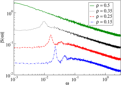
Figure 3: (Color online.) Fourier transform $|S(\omega)|$ of $S(0,t)$ for one-dimensional driven lattice gases (TASEP) with $L=400$, at various densities $\rho=0.15$, $0.25$, $0.35$, and $0.5$. The curves are vertically shifted to separate them and show the peaks. In each case, the data were averaged over 800,000 realizations.

In order to extract the period of the recurrent density fluctuations, we Fourier transform the auto-correlation function, $S(\omega)=\int S(0,t)e^{i\omega t}dt$. The first peak in $|S(\omega)|$ is caused by the movement of a density fluctuation at a frequency $\omega_{c}=2\pi/T_{c}$, see Fig. 3. At low densities, higher harmonics are also visible. The characteristic frequency $\omega_{c}$ vanishes as the density approaches $1/2$. We finally mention previous work by Adams et al. adams and Cook and Zia cook who studied density oscillations in the open TASEP that are also caused by fluctuations that traverse the entire system. Gupta et al. studied similar oscillations in the displacement variance for tagged particles oscillate . Exact calculations of the spectral gap yield evidence of oscillations as well spec_osc2 ; spec_osc1 ; kirone_rev , which are also found in exact solutions for the time-dependent conditional probabilities and single particle correlation function exact3 .

III.2 Finite-size scaling

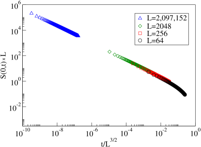
Figure 4: (Color online.) Finite-size scaling for the density auto-correlation function for $L=64$ (data averaged over 80,000 realizations), $L=256$ (10000 realizations), $L=2048$ (40,000 realizations), and $L=2,097,152$ (60 realizations).

Next we analyze the finite-size scaling properties of the density auto-correlation function for the driven lattice gas with exclusion in one dimension (TASEP). The expected finite-size scaling form is readily obtained from the general expression (9) by setting $L=b^{-(1+\Delta)}$, and omitting the transverse space directions:

$$S(x,t)=L^{-1}S_{\rm FS}\Bigl{(}x/L,t/L^{z_{\parallel}}\Bigr{)}.$$ (20)

Taking $x\to 0$ we find for the auto-correlation function

$$S(0,t)=L^{-1}S_{\rm FS}\Bigl{(}t/L^{z_{\parallel}}\Bigr{)}.$$ (21)

As shown in Fig. 4, the finite-size scaling form (21) produces satisfactory data collapse with $z_{\parallel}=3/2$ for our simulation results for vastly different lattice sizes ranging from $L=64$ to $L=2,097,152$. At $t/L^{z_{\parallel}}\approx 0.1$ one observes the expected finite-$L$ cutoff from the scaling form (21), as the return time $t_{r}$ is approached. We note that earlier work has studied the finite-size scaling properties of the TASEP with open boundaries in the maximum current phase which is equivalent to the periodic case; however much smaller system sizes of respectively $L=50$ and $L=257$ were utilized by Pierobon et al. Pier and Juhász and Santen Juh .

III.3 Long-time properties

III.3.1 Scaling functions

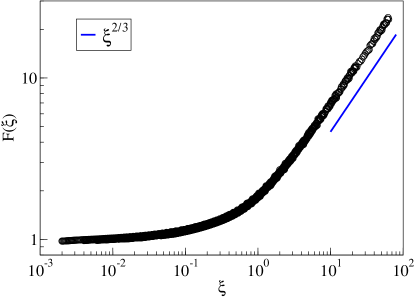
Figure 5: (Color online.) Double-logarithmic plot of the scaling function $F(\xi)$, defined in Eq. (22), obtained from Monte Carlo simulations in a driven lattice gas on a ring of length $L=2000$, with $x\in[0,64]$ and $t\in[0,64]$. The data are averaged over 200 realizations.

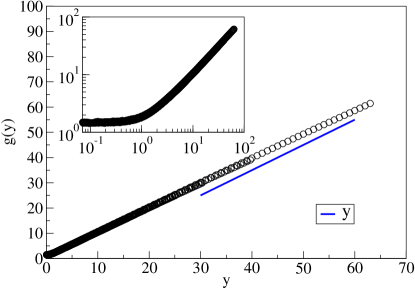
Figure 6: (Color online.) The scaling function $g(y)$ defined in Eq. (23), from the same data as in Fig. 5 ($L=2000$, $x\in[0,64]$, and $t\in[0,64]$, averaged over 200 realizations). The inset represents the same data in a double-logarithmic plot to display the crossover to a constant as $y\to 0$.

We now address the stationary height-height correlation function (13) in one dimension, and explicitly determine associated scaling functions. Setting $b=1/|x|$, and recalling $\alpha=1/2$ and $z_{\parallel}=3/2$, Eq. (15) becomes uwehwa

$$C(x,t)\propto|x|F(\xi),\ \xi=t/|x|^{3/2}\ ,$$ (22)

whereas equivalently the matching condition $b=t^{-1/z_{\parallel}}$ leads to spohnlong

$$C(x,t)\propto t^{2/3}g(y),\ y=x/t^{2/3}\ .$$ (23)

Consistency then requires that

$$F(\xi)\propto\xi^{2/3},\ g(y)\propto|y|$$ (24)

for large arguments $\xi\gg 1$ and $y\gg 1$. Figures 5 and 6 depict the scaling functions $F(\xi)$ and $g(y)$ as obtained from our simulations for a driven periodic lattice gas with exclusion on a ring of length $L=2000$. The Monte Carlo data nicely confirm the relations (24). The crossover from $F(\xi)=\rm const.$ for small arguments $\xi$ to the asymptotic behavior $\sim\xi^{2/3}$ visible in Fig. 5 can be compared with the numerical solution of the mode-coupling equations depicted in Fig. 2 of Ref. uwehwa and the simulation results shown in Fig. 2 of Ref. monte_1 . The mode-coupling approximation appears to predict sharper crossover features, with $F(\xi)$ remaining constant until $\xi\approx 0.5$, where our data already indicate a noticeable curvature in the scaling function $F$. The simulation data in Ref. monte_1 , obtained for much larger systems with $L=1048576$, also display sharper crossover features than our data for $L=2000$.

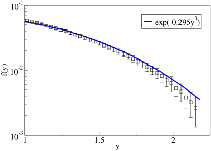
Figure 7: (Color online.) Logarithmic plot of the scaling function $f(y)$, defined in Eq. (25), for $L=2000$, with $x\in[0,256]$ and $t\in[0,256]$, with the data averaged over 400,000 realizations. The error bars indicate one standard deviation.

Combining Eqs. (14) and (23), we recover the scaling form (10) for the density-density correlation function in one dimension,

$$S(x,t)\propto t^{-2/3}f(y).$$ (25)

Our Monte Carlo simulation data for the scaling function $f(y)$, measured by averaging over a very large number of realizations, are plotted in Fig. 7. Within the error bars, our data are in reasonable aggreement with the stretched exponential function $f(y)\propto\exp(-cy^{3})$, where $c=0.295(5)$, that was computed in Ref. spohnlong .

III.3.2 Local exponent

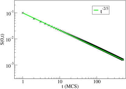
Figure 8: (Color online.) Double-logarithmic plot of the stationary auto-correlation function $S(0,t)$ for a one-dimensional driven lattice gas of length $L=2048$ with exclusion. The data are averaged over 40,000 realizations. The light green line represents a power law with exponent $-2/3$.

In Fig. 8 we plot the density auto-correlation function $S(0,t)$ as obtained from our simulations for a one-dimensional driven lattice gas with exclusion with $L=2048$ (see also Fig. 4). From Eq. (11) with $\zeta=1/z_{\parallel}=2/3$, we expect the asymptotic long-time power law $S(0,t)\sim t^{-2/3}$, which fits the Monte Carlo data well for $t>100$ on the double-logarithmic plot. The approach to the expected asymptotic power law auto-correlation decay can be carefully probed by studying the local effective exponent $\zeta_{\rm eff}(t)$ defined in Eq. (12).

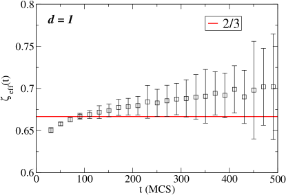
Figure 9: (Color online.) The local auto-correlation exponent (12) obtained from Monte Carlo simulation data for a one-dimensional driven lattice gases with length $L=2048$ and for $\rho=1/2$. The data are averaged over 40,000 realizations. The error bars represent one standard deviation, and the (red) horizontal line the asympotic value $2/3$.

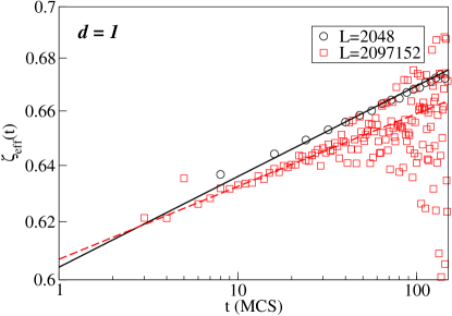
Figure 10: (Color online.) Time dependence of the local exponent $\zeta_{\rm eff}(t)$ for one-dimensional driven lattice gases with $L=2048$ (black circles, data averaged over 40,000 realizations) and $L=2097152$ (red squares, 60 realizations).

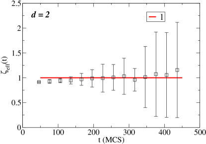
Figure 11: (Color online.) The effective exponent $\zeta_{\rm eff}(t)$, Eq. (17), for a two-dimensional driven lattice gas with $L_{x}=L_{y}=100$ and $\rho=1/2$. The data are averaged over 600,000 realizations. The error bars indicate one standard deviation, and the (red) horizontal line the asympotic value $1$.

Figure 9 shows that the local exponent increases with time and in fact surpasses the asymptotic value $2/3$, indicated by the horizontal line. In order to demonstrate that this is actually a finite-size effect, albeit a quite unusual one, we display in Fig. 10 a comparison of simulation data for the time dependence of the effective exponent for systems of sizes $L=2048$ and $L=1024\times 2048=2097152$ on a logarithmic time scale. Even in the much larger lattice, $\zeta_{\rm eff}(t)$ still rises beyond the asymptotic exponent value $\zeta=2/3$ of the infinite system, yet at later time. Since we have not observed this overshooting in unbiased lattice gases with exclusion, it is clearly a consequence of the non-equilibrium drive. We note that the extremely slow crossover towards the asymptotic temporal power law has been recorded before in a model of reconstituting dimers that can be mapped to the TASEP MBarma .

We next compare the behavior of the local auto-correlation exponent $\zeta_{\rm eff}(t)$ for the one-dimensional driven lattice gas with its two- and three-dimensional counterparts, see Figs. 11 and 12. In each case, the system is half-filled ($\rho=1/2$), and the hopping rates are equal in each direction transverse to the drive, but set totally asymmetric parallel to the drive. For a two-dimensional driven lattice gas ($L_{x}=L_{y}=100$), we depict the effective exponent as defined in Eq. (17) in Fig. 11, and analogous results for the three-dimensional case are shown in Fig. 12. Since we are at or above the critical dimension $d_{c}=2$, respectively, the asymptotic value is $\zeta=d/2$. Indeed, the local exponent $\zeta_{\rm eff}(t)$ quickly relaxes to $1$ for $d=2$ and $3/2$ for $d=3$, and never surpasses these expected asymptotic values. The anomalously slow convergence and unusual finite-size behavior in one dimension are consequently caused by the strong out-of-equilibrium correlations present only for $d<d_{c}$.

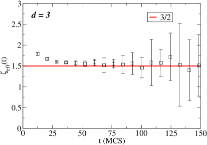
Figure 12: (Color online.) The local exponent $\zeta_{\rm eff}(t)$ for a three-dimensional driven lattice gas with $L_{x}=L_{y}=L_{z}=50$ and $\rho=1/2$. The data are averaged over 1,320,000 realizations. The error bars indicate one standard deviation, and the (red) horizontal line the asympotic value $3/2$.

Up to this point, we have provided results only for driven lattice gases with zero backward hopping rate along the drive direction (TASEP in one dimension). Assigning the forward hopping probability $p$ and backward probability $q$, we can define the bias $\Gamma=p-q=2p-1$. As long as $1/2<p<1$ and $0<\Gamma<1$ (ASEP), a macroscopic particle current persists, the system remains out of equilibrium, and one expects qualitatively the same behavior as for maximum bias or drive, $p=\Gamma=1$. Thus, at long times, the temporal decay of the density auto-correlation function should be described by a power law with exponent $\zeta=2/3$ in one dimension, for any non-zero value of the hopping bias $\Gamma$. However, note that this statement is valid at asympotically long times for sufficiently large systems, and a simple power-law decay will not necessarily be observable in finite systems with weak bias. Monte Carlo simulation data for one-dimensional driven lattice gases with various bias values are shown in Fig. 13. As can be seen, the local exponent $\zeta_{\rm eff}(t)$ relaxes increasingly slowly towards its asymptotic value $2/3$ as the bias is reduced. The figure illustrates that for low bias and at short times, the density auto-correlation decay rather follow the symmetric exclusion process (SEP) relaxation, for which $\zeta=1/2$. For example, for $\Gamma=0.2$ a distinct decrease in the local exponent is observed for $t<30$, later followed by a very slow increase.

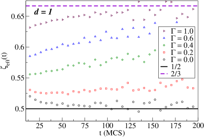
Figure 13: (Color online.) Local auto-correlation exponent $\zeta_{\rm eff}(t)$ for one-dimensional driven lattice gases (ASEP) with different hopping biases $\Gamma=1.0$ (TASEP), $0.6$, $0.4$, $0.2$ (all ASEP), and $0.0$ (vanishing drive, SEP); $L=4096$ and $\rho=1/2$. The data are averaged over 5,000,000 realizations each.

IV Non-equilibrium relaxation

IV.1 Transitions between steady states

Let us finally consider transient relaxation properties of driven lattice gases with exclusion. For example, starting from a steady state obtained with a specified set of hopping probabilites $p$ and $q=1-p$, we may wish to understand how the system responds to a sudden change of these probabilities to new values $p^{\prime}$ and $q^{\prime}=1-p^{\prime}$. However, recall that the non-equilibrium steady state probability distribution (4) is independent of the hopping probabilities. This means that statistically the stationary configurations before and after the sudden bias change are indistingishable. As a consequence, no slow relaxation processes follow the change of hopping probabilities. As we have confirmed with our Monte Carlo simulations, any macroscopic observables such as the mean particle current assume their new stationary values essentially instantaneously after the bias reset.

IV.2 Strongly correlated initial conditions

In order to construct initial conditions that generate non-stationary relaxation with broken time translation invariance, we consider the mapping of the TASEP to a surface growth problem in the KPZ universality class meak . In the growth model, one obtains slow relaxation towards the stationary state if the process is initiated with a flat surface $h(x,0)=0$ everywhere, and roughening subsequently commences on small length scales $\sim t^{1/z_{\parallel}}$. In the TASEP picture, this initial state is accomplished at half-filling $\rho=1/2$ by placing the particles alternatingly on every other site. The mean-square interface width of the corresponding finite one-dimensional growth model can be obtained from our TASEP Monte Carlo data on a ring of length $L$ via Eq. (1),

$$w(L,t)^{2}=\Big{\langle}h(x,t)^{2}\Big{\rangle}_{L}=\frac{1}{L}\displaystyle\sum_{x=1}^{L}\Bigl{[}x-2\displaystyle\sum_{y=1}^{x}n(y,t)\Bigr{]}^{2},$$ (26)

where $w(L,0)^{2}=0$. The standard finite-size scaling relation for the interface width reads family

$$w(L,t)=L^{\alpha}W(t/L^{z_{\parallel}}),$$ (27)

with $\alpha=1/2$ and $z_{\parallel}=3/2$ in the KPZ universality class, which implies the initial growth law $w(L,t)\sim t^{\alpha/z_{\parallel}}=t^{1/3}$, valid up to times $t\approx L^{z_{\parallel}}$ kpz . Our Monte Carlo simulation results nicely confirm the scaling relation (27), as evidenced in Fig. 14 by the satisfactory data collapse for various system sizes with the expected scaling exponents (compare also the analogous mode-coupling results in Fig. 3 of Ref. uwehwa , and the simulation data shown in Fig. 1 of Ref. Queiroz ). Our measurements yield an initial growth exponent $0.30$, slightly different from the expected value $1/3$, likely caused by sizeable corrections to scaling in our data. Our finite size scaling plot of the width matches the simulation data of Ref. Queiroz .

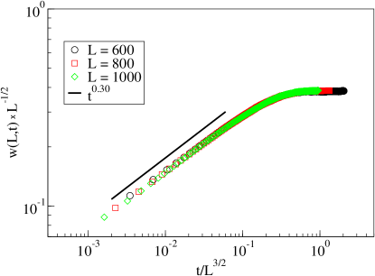
Figure 14: (Color online.) Finite-size scaling for the interface width of the one-dimensional growth model that corresponds to the TASEP, for system sizes $L=600$, $800$, and $1000$, see Eq. (27). The data are averaged over 50,000 realizations each.

Starting from the highly correlated initial configuration of alternatingly occupied sites in the TASEP that corresponds to a flat surface in the growth model representation, time translation invariance is broken during the slow approach to the stationary regime. The density-density or height-height correlation functions then depend explicitly on both time arguments $t$ and $t^{\prime}$. Henceforth we shall refer to the second argument as waiting time $s$, and consider the short-time scaling limit $s\ll t$ pleimbook . By means of a careful renormalization group analysis, Krech krech established the following scaling form for the two-time height-height correlation function in this limit:

$$C_{\rm IS}(x,t,s\ll t)=\left(\frac{s}{t}\right)^{\theta}|x|^{2\alpha}F(t/x^{z_{\parallel}}),$$ (28)

which generalizes Eq. (22) that is valid in the stationary regime. Here, the initial slip exponent $\theta=(d+4)/z_{\parallel}-2$ can be expressed in terms of the standard dynamic scaling exponent $z$. This follows since the initial-time surface does not induce any novel singularities, as a consequence of the momentum dependence of the nonlinear vertex in the KPZ problem, and thus no additional renormalizations are required.

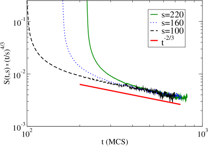
Figure 15: (Color online.) Scaling plot for the density auto-correlation function for a one-dimensional driven lattice gas (TASEP) with length $L=1000$ and density $\rho=1/2$ in the non-equilibrium relaxation regime, see Eq. (30), measured for waiting times $s=100$, $160$, and $220$. The data are averaged over 60,000 realizations.

In one dimension, the renormalization group predicts $\theta=4/3$. For the TASEP density-density correlation function, we obtain by means of Eq. (14)

$$S_{\rm IS}(x,t,s\ll t) =\left(\displaystyle\frac{s}{t}\right)^{\theta}|x|^{2\alpha-2}f(t/x^{z_{\parallel}})$$ (29)

$$=\left(\displaystyle\frac{s}{t}\right)^{4/3}|x|^{-1}f(t/x^{3/2}).$$

In order to arrive at the temporal behavior of the auto-correlation function, we must require that the scaling function $f(\xi)\sim\xi^{-2/3}$ as its argument $\xi\to\infty$, whence

$$S_{\rm IS}(0,t,s\ll t)=\left(\frac{s}{t}\right)^{4/3}t^{-2/3}.$$ (30)

Our Monte Carlo auto-correlation data displayed in Fig. 15, obtained for various waiting times $s$, convincingly confirm the scaling predicted by Eq. (30) for $s\ll t$.

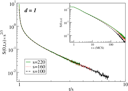
Figure 16: (Color online.) Simple aging scaling plot, see Eq. (19), for the density-density auto-correlation function for a one-dimensional driven lattice gas (TASEP) of length $L=1000$, at density $\rho=1/2$, obtained from Monte Carlo simulation data with different waiting times $s=100$, $160$, and $220$. The data sets are averaged over 60,000 realizations each.

Finally, we explore the scaling properties of the two-time height and density auto-correlation functions in the physical aging regime. As shown for the KPZ growth model, no additional renormalizations, and hence no independent new scaling exponents are required in the non-stationary relaxation regime in one dimension krech . Since this is essentially a consequence of the underlying conserved dynamics, we surmise that we can generalize the scaling laws (15) and (9) to

$$C(x,t,s)=b^{-2\alpha}C(bx,b^{z_{\parallel}}t,b^{z_{\parallel}}s),$$ (31)

$$S(x,t,s)=b^{d+\Delta}S(b{\vec{x}}_{\perp},b^{1+\Delta}x_{\parallel},b^{z}t,b^{z}s),$$ (32)

with $z=z_{\parallel}(1+\Delta)$ and $2z(1-\alpha)=z_{\parallel}(d+\Delta)$. Letting $x\to 0$ and setting $b=s^{-1/z_{\parallel}}$, Eq. (31) yields for the growth model height-height auto-correlation function

$$C(0,t,s)=s^{2\alpha/z_{\parallel}}f_{C}(t/s)=s^{2/3}f_{C}(t/s).$$ (33)

Recent Monte Carlo simulations have confirmed this simple aging scaling scenario pleimbook for the KPZ universality class krug ; michelnew ; A4 ; yenglobal . In a similar vein, for the density-density auto-correlation function in the driven lattice gas, via matching $b=s^{-1/z}$ we obtain Eq. (19), with the scaling exponent $\zeta$ given in Eq. (11). Figure 16 confirms the simple aging scenario according to Eq. (19) through the nice data collapse of our Monte Carlo simulation results for various waiting times in one dimension, where $\zeta=2/3$. We have also performed driven lattice gas simulations in two and three dimensions with alternating particle initial conditions on periodic lattices. As demonstrated in Figs. 17 and 18, we obtain simple-scaling data collapse with the expected scaling exponent $\zeta=1$ for $d=2$ and $\zeta=3/2$ for $d=3$, respectively.

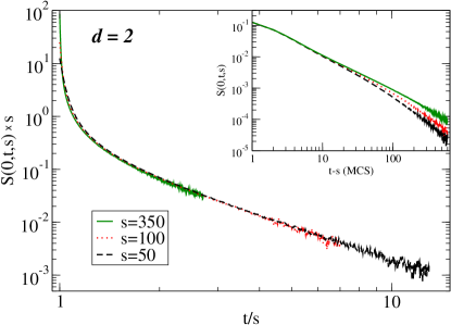
Figure 17: (Color online.) Density auto-correlation function for a two-dimensional driven lattice gas of size $L_{x}=L_{y}=128$ for density $\rho=1/2$ in the aging scaling regime for waiting times $s=50$, $100$, and $350$. Each data set is averaged over 160,000 realizations.

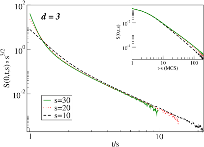
Figure 18: (Color online.) Density auto-correlation function for a three-dimensional driven lattice gas of size $L_{x}=L_{y}=L_{z}=20$ for density $\rho=1/2$ in the aging scaling regime for waiting times $s=10$, $20$, and $30$. Each data set is averaged over 4,200,000 realizations.

V Conclusion

We have performed extensive precise Monte Carlo simulations of driven lattice gases with exclusion on periodic lattices, and studied in detail the behavior of the density correlations in one, two, and three dimensions.

For the one-dimensional case, we have investigated interesting recurrence oscillations away from half-filling, and explained the minimum value in the density auto-correlation function observed for small systems. We also studied how varying the hopping bias in the ASEP affects the crossover to the long-time power law decay of the density auto-correlation function. While our large-scale simulations confirm standard finite-size scaling behavior, the effective exponent that describes the temporal decay of the auto-correlations approaches the asymptotic value exceedingly slowly, even for the TASEP, and displays very unusual finite-size corrections to scaling. Our Monte Carlo simulation results confirm all expected non-trivial scaling exponents for the driven lattice gas, in accord with the scaling properties of equivalent growth models in the KPZ universality class. This includes predictions for the simple aging scaling scenario during the non-stationary relaxation from strongly correlated initial conditions. Our data thus support the assertion that in driven lattice gas with exclusion, the entire universal scaling regime is governed by a single non-trivial exponent $\Delta$ (or equivalently, $z_{\parallel}$ or $\zeta$). Specifically, no novel scaling exponent is required to capture non-equilibrium aging properties in this system. We have moreover numerically determined several different universal scaling functions.

We extended our Monte Carlo simulations to two and three dimensions. Aside from logarithmic corrections at the critical dimension $d_{c}=2$, we have confirmed mean-field scaling behavior for the density auto-correlation function in both the stationary long-time and the non-stationary aging regimes.

- (1) B. Schmittmann and R. K. P. Zia, Statistical Mechanics of Driven Diffusive Systems edited by C. Domb and J. L. Lebowitz (Academic Press, London, 1995).
- (2) T. Halpin-Healy and Y.-C. Zhang, Phys. Rep. 254, 215 (1995).
- (3) B. Derrida, Phys. Rep. 301, 65 (1998).
- (4) G. M. Schütz, Phase Transitions and Critical Phenomena Volume 19 edited by C. Domb and J. L. Lebowitz (Academic Press, London, 2000).
- (5) K. Mallick, J. Stat. Mech. , P01024 (2011).
- (6) D. Dhar, Phase Transitions 9, 51 (1987).
- (7) L.-H. Gwa and H. Spohn, Phys. Rev. Lett. 68, 725 (1992).
- (8) L.-H. Gwa and H. Spohn, Phys. Rev. A 46, 844 (1992).
- (9) O. Golinelli and K. Mallick, J. Phys. A: Math. Gen. 37, 3321 (2004).
- (10) D. Kim, Phys. Rev. E 52, 3512 (1995).
- (11) O. Golinelli and K. Mallick, J. Phys. A: Math. Gen. 38, 1419 (2005).
- (12) G. Schütz, J. Stat. Phys. 88, 427 (1997).
- (13) V. B. Priezzhev, Phys. Rev. Lett. 91, 050601 (2003).
- (14) D. Forster, D. R. Nelson, and M. J. Stephen, Phys. Rev. A 16, 732 (1977).
- (15) M. Kardar, G. Parisi, and Y.-C. Zhang, Phys. Rev. Lett. 56, 889 (1986).
- (16) H. K. Janssen and B. Schmittmann, Z. Phys. B 63, 517 (1986).
- (17) H. van Beijeren, R. Kutner, and H. Spohn, Phys. Rev. Lett. 54, 2026 (1985).
- (18) T. Hwa and E. Frey, Phys. Rev. A 44, R7873 (1991).
- (19) E. Frey, U. C. Täuber, and T. Hwa, Phys. Rev. E 53, 4424 (1996).
- (20) F. Colaiori and M. A. Moore, Phys. Rev. Lett. 86, 3946 (2001).
- (21) F. Colaiori and M. A. Moore, Phys. Rev. E 63, 057103 (2001).
- (22) B. Hu and G. Tang, Phys. Rev. E 66, 026105 (2002).
- (23) L. Canet and M. A. Moore, Phys. Rev. Lett. 98, 200602 (2007).
- (24) F. Colaiori and M. A. Moore, Phys. Rev. E 65, 017105 (2001).
- (25) M. Prähofer and H. Spohn, J. Stat. Phys. 115, 255 (2004).
- (26) E. Katzav and M. Schwartz, Phys. Rev. E 69, 052603 (2004).
- (27) J. Krug, P. Meakin, and T. Halpin-Healy, Phys. Rev. A 45, 638 (1992).
- (28) T. Nattermann and L.-H. Tang, Phys. Rev. A 45, 7156 (1992).
- (29) H. C. Fogedby, J. Phys.: Condens. Matter 14, 1557 (2002).
- (30) P. L. Ferrari and H. Spohn, Commun. Math. Phys. 265, 1 (2006).
- (31) M. Krech, Phys. Rev. E 55, 668 (1997).
- (32) M. Henkel and M. Pleimling, Ageing and Dynamical Scaling Far from Equilibrium, Nonequilibrium phase transitions Vol. 2 (Springer, Dordrecht, 2010).
- (33) H. Kallabis and J. Krug, Europhys. Lett. 45, 20 (1999).
- (34) S. Bustingorry, J. Stat. Mech. , P10002 (2007).
- (35) M. Henkel, J. D. Noh, and M. Pleimling, Unpublished (2010).
- (36) Y.-L. Chou and M. Pleimling, J. Stat. Mech , P08007 (2010).
- (37) A. Röthlein, F. Baumann, and M. Pleimling, Phys. Rev. E 74, 061604 (2006).
- (38) S. Bustingorry, L. F. Cugliandolo, and J. L. Iguain, J. Stat. Mech., P09008 (2007).
- (39) Y.-L. Chou, M. Pleimling, and R. K. P. Zia, Phys. Rev. E 80, 061602 (2009).
- (40) T. Sasamoto, J. Phys. A: Math. Gen. 38, L549 (2005).
- (41) A. Borodin, P. Ferrari, M. Prähofer, and T. Sasamoto, J. Stat. Phys. 129, 1055 (2007).
- (42) A. M. Povolotsky and V. B. Priezzhev, J. Stat. Mech. , P08018 (2007).
- (43) T. Sasamoto, Eur. Phys. J. B 64, 373 (2008).
- (44) M. E. Newman and G. T. Barkema, Monte Carlo Methods in Statistical Physics (Oxford University Press, Oxford, 1999).
- (45) A. B. Bortz, M. H. Kalos, and J. L. Lebowitz, J. Comput. Phys. 17, 10 (1975).
- (46) P. Meakin, P. Ramanlal, L. M. Sander, and R. C. Ball, Phys. Rev. A 34, 5091 (1986).
- (47) M. Prähofer and H. Spohn, Current fluctuations for the totally asymmetric simple exclusion process, in In and Out of Equilibrium, Progr. Probab. No. 51, pp. 185–204, Birkhäuser, Boston, MA, 2002.
- (48) D. A. Adams, R. K. P. Zia, and B. Schmittmann, Phys. Rev. Lett. 99, 020601 (2007).
- (49) L. J. Cook and R. K. P. Zia, J. Stat. Mech. , P07014 (2010).
- (50) S. Gupta, S. N. Majumdar, C. Godrèche, and M. Barma, Phys. Rev. E 76, 021112 (2007).
- (51) M. Makhanova and V. Priezzhev, Theoret. and Math. Phys. 146, 421 (2006).
- (52) P. Pierobon, A. Parmeggiani, F. von Oppen, and E. Frey, Phys. Rev. E 72, 036123 (2005).
- (53) R. Juhsz and L. Santen, J. Phys. A: Math. Gen. 37, 3933 (2004).
- (54) L. H. Tang, J. Stat. Phys. 67, 819 (1992).
- (55) M. Barma, M. D. Grynberg, and R. B. Stinchcombe, J. Phys-Condens. Mat. 19, 065112 (2007).
- (56) F. Family and T. Vicsek, J. Phys. A: Math. Gen. 18 (1985).
- (57) S. L. A. de Queiroz and R. B. Stinchcombe, Phys. Rev. E 78, 031106 (2008).