Stochastic Gravitational Wave Background from Neutron Star r-mode Instability Revisited

Abstract

We revisit the possibility and detectability of a stochastic gravitational wave (GW) background produced by a cosmological population of newborn neutron stars (NSs) with r-mode instabilities. The NS formation rate is derived from both observational and simulated cosmic star formation rates (CSFRs). We show that the resultant GW background is insensitive to the choice of CSFR models, but depends strongly on the evolving behavior of CSFR at low redshifts. Nonlinear effects such as differential rotation, suggested to be an unavoidable feature which greatly influences the saturation amplitude of r-mode, are considered to account for GW emission from individual sources. Our results show that the dimensionless energy density $\Omega_{\rm{GW}}$ could have a peak amplitude of $\simeq(1-3.5)\times 10^{-8}$ in the frequency range $(200-1000)$ Hz, if the smallest amount of differential rotation corresponding to a saturation amplitude of order unity is assumed. However, such a high mode amplitude is unrealistic as it is known that the maximum value is much smaller and at most $10^{-2}$. A realistic estimate of $\Omega_{\rm{GW}}$ should be at least 4 orders of magnitude lower ($\sim 10^{-12}$), which leads to a pessimistic outlook for the detection of r-mode background. We consider different pairs of terrestrial interferometers (IFOs) and compare two approaches to combine multiple IFOs in order to evaluate the detectability of this GW background. Constraints on the total emitted GW energy associated with this mechanism to produce a detectable stochastic background (a SNR of 2.56 with 3-year cross correlation) are $\sim 10^{-3}\hskip 2.84526ptM_{\odot}c^{2}$ for two co-located advanced LIGO detectors, and $2\times 10^{-5}\hskip 2.84526ptM_{\odot}c^{2}$ for two Einstein Telescopes. These constraints may also be applicable to alternative GW emission mechanisms related to oscillations or instabilities in NSs depending on the frequency band where most GWs are emitted.

1 Introduction

A stochastic gravitational wave background (SGWB) is a target for gravitational wave (GW) interferometers (IFOs). It could have two very different origins. It may result from a large variety of cosmological processes developed in the very early universe, such as amplification of quantum vacuum fluctuations, phase transitions, cosmic strings, etc. (see, e.g., Maggiore 2000; Buonanno 2003 for reviews). Additionally, an astrophysical GW background (AGWB) is expected to be produced by the superposition of a large number of unresolved sources since the beginning of star formation (Schneider et al. 2000; Regimbau & Mandic 2008). There have been a host of literatures dedicated to the studies of various AGWB sources, such as core collapse supernovae (CCSNe) Blair & Ju (1996), leading to the formation of neutron stars (NSs) (Coward et al. 2001; Howell et al. 2004; Buonanno et al. 2005) or black holes (BHs) (Ferrari et al. 1999a; de Araujo et al. 2004; Pereira & Miranda 2009), phase transitions in NSs (Sigl 2006; de Araujo & Marranghello 2009), coalescing compact binaries consisting of NSs and/or BHs (Schneider et al. 2001; Farmer & Phinney 2002; Regimbau & de Freitas Pacheco 2006a; Regimbau & Chauvineau 2007), magnetars (Regimbau & de Freitas Pacheco 2006b) and population III stars (Sandick et al. 2006; Suwa et al. 2007; Marassi et al. 2009) among others.

In this paper we revisit the possibility that the r-mode instabilities in newly born NSs could form a SGWB. NSs, having long been considered to be likely observational sources for GW detection, emit gravitational radiation in a number of ways, for example, through CCSNe, inspiralling compact binaries, rotating deformed stars, oscillations and instabilities Andersson et al. (2010). First postulated more than ten years ago (Andersson 1998; Friedman & Morsink 1998), the r-mode instability has been attracting increased attention due to the fact that it is driven unstable by GW emission and it can be active for a wide range of core temperatures and angular velocities (Lindblom et al. 1998; Andersson & Kokkotas 2001; Andersson et al. 2003). Early estimate indicated an energy equivalent to roughly $1\%$ of a solar mass is radiated in GWs (Andersson et al. 1999) as an initially rapidly rotating star spins down. This led to an expectation of a SGWB produced by a cosmological population of young rapidly rotating NSs with closure density $h^{2}\Omega_{\rm{GW}}$ peaking at $\sim 10^{-8}$ of the present-day critical energy density of the universe Owen et al (1998); Ferrari et al. 1999b .

The most important aspect of the r-mode intability is the largest amplitude (often called the saturation amplitude $\alpha$) that the perturbation can grow to. This maximum amplitude determines how fast the NS spins down and whether the associated GW emission will be detectable (either in terms of single event or a stochastic background). In Owen et al. (1998) and then Ferrari et al. (1999b) it was taken to be of order unity (there were no estimates of this maximum at that time). Later more detailed (both analytical and numerical) studies seriously questioned the potential of the instability as well as the efficiency of GW emission (Rezzolla et al. 2000; Ho & Lai 2000; Lindblom et al. 2000; Rezzolla et al. 2001a, 2001b; Lindblom & Owen 2002). On the one hand, it was suggested that energy transfer to other stellar inertial modes can significantly reduce the saturation amplitude of r-mode Schenk et al. (2002); Morsink (2002); Brink et al. (2004). Arras et al. (2003) tested nonlinear coupling between stellar inertial modes and revealed much lower values of saturation amplitude ($\alpha\sim 10^{-4}-10^{-1}$). Then a specific resonant three-mode coupling between the r-mode and the pair of fluid modes was identified to be responsible for the catastrophic decay of large-amplitude r-modes and a perturbative analysis of the decay rate suggested a maximum dimensionless saturation amplitude $\alpha_{\rm{max}}<10^{-3}-10^{-2}$ Lin & Suen (2006). More recently Bondarescu et al. (2009) examined the 3-mode coupling between the r-mode and two other inertial modes and showed that the r-mode evolution can progress in a number of different directions depending on unknown properties of the viscosity, leading to very complex consequent mode evolution and the associated GW signal.

On the other hand, differential rotation, first suggested by Rezzolla et al. (2000, 2001a, 2001b), is an unavoidable feature of nonlinear r-modes (Stergioulas & Font 2001; Lindblom et al. 2001; Sá 2004). Small values of $\alpha$ mentioned above are also supported by studies on the role of differential rotation, causing large scale drift of fluid elements, in the nonlinear evolution of r-modes (Sá & Tomé 2005). In particular they parametrize the initial amount of differential rotation by $K$ and then relate the parameter $K$ to the largest amplitude that the r-mode can grow to. In this paper we will use the characteristic GW amplitude given by Sá & Tomé (2006) to account for the average source spectrum. The adopted GW amplitude, parametrized by parameter $K$, in fact scales with the saturation amplitude $\alpha$. Below we will discuss the influence of this quantity on the r-mode background.

In addition to the average source spectra, the properties of AGWB also depend on GW source formation rate. Studies of cosmic star formation rate (CSFR) allow estimation of the birth rate of NSs. In the last decade our knowledge of cosmic star formation has been greatly improved due to advances in astronomical observation and hydrodynamic simulation. Here we take into account both observational and simulation-based CSFR models to obtain the NS formation rate and discuss their effects on the resultant GW background. In particular, we will investigate the role of the maximal redshift of different CSFR models in our results.

The high-frequency window of GW spectrum ($10~{}\rm{Hz}\leq f\leq$ a few kHz) is open today through pioneering efforts of the first-generation terrestrial IFOs, such as Laser Interferometer Gravitational Wave Observatory (LIGO) (Abramovici et al. 1992) in Livingston (LIGOL) and in Hanford (LIGOH), Virgo (Caron et al. 1997) near Pisa, GEO600 (Lück et al. 1997) in Hanover and TAMA300 (Ando et al. 2001) at Tokyo. Although GWs were not detected, an observational upper limit ($\Omega_{\rm{GW}}<6.9\times 10^{-6}$) was placed on the energy density of SGWB at around 100 Hz, exceeding previous indirect limits from the Big Bang Nucleosynthesis and the cosmic microwave background Abbott et al. (2009). In the future the SGWB from NS r-mode instability, among others, may offer an important detection target for the proposed second and third generation detectors represented by advanced LIGO (or advanced Virgo) and the Einstein Telescope (ET) respectively.

Detectors throughout the world can act as a network in order to improve the detection ability to the SGWB. Two approaches of combining 2N IFOs are proposed in Allen & Romano (1999): (i) correlating the outputs of a pair of IFOs, then combining the multiple pairs, and (ii) directly combining the outputs of 2N IFOs. For any given real IFOs it is necessary to compare these two optimal approaches of detecting the SGWB. Cella et al. (2007) has shown that the approach of combining multiple pairs of IFOs using Virgo, LIGO and GEO can improve the detection ability to the SGWB by simulating an isotropic GW background with an astrophysically-motivated spectral shape. Fan & Zhu (2008) compared the detection ability of the two approaches for stochastic GWs from string cosmology.

Detectability of the r-mode background are demonstrated here by calculating signal-to-noise ratios (SNRs) for pairs of currently operating IFOs and advanced detectors at their design sensitivities. We also consider two approaches of combining 4 real IFOs to examine how many improvements can be obtained. The organization of this paper is as follows. In Section 2 we review works on the determination of CSFR and present five CSFR models. In Section 3 we derive the NS formation rate as a function of redshift using the adopted CSFR models. Then by combining the source formation rate from Section 3 and the characteristic GW amplitude of individual events, spectral properties of the r-mode stochastic background are investigated in Section 4. We will discuss the detectability of r-mode background in Section 5 and finally Section 6 is devoted to our conclusions.

Throughout the paper, the so-called 737 $\Lambda$CDM cosmology is assumed with $H_{0}=100h\cdot\rm{km}\hskip 1.42262pt\rm{s}^{-1}\hskip 1.42262pt\rm{Mpc}^{-1}$ with $h=0.7$ and $\Omega_{m}=0.3$, $\Omega_{\Lambda}=0.7$ (e.g., Komatsu et al. 2009).

2 Cosmic star formation rate

The CSFR, which has tight connection with GW event rate, is of intense interest to many fields of astrophysics. For many years effort has gone into studying the cosmic star formation history (see, e.g., Madau et al. 1996; Hopkins 2004; Wilkins et al. 2008). Since CSFR is not a directly observable quantity, usually the rest-frame ultraviolet (UV) light is considered to be an indicator (see Calzetti 2008 and references therein for details about CSFR indicators) of star formation because it is mainly radiated by short-lived massive stars. With the help of Hubble Space Telescope (HST) and other large telescopes, galaxy luminosity density of rest-frame UV radiation is studied, and then converted into CSFR density through the adoption of a universal stellar initial mass function (IMF) to calculate the conversion factor. Many authors have developed parameterized fits to the expected evolution of the CSFR with redshift. Firstly, following Porciani & Madau (2001), we adopt three different forms which model the CSFR density for redshifts up to $z\approx 4$:

$$\dot{\rho}_{\ast}(z)_{i}=1.67C_{i}h_{65}F(z)G_{i}(z)\quad M_{\odot}\hskip 1.42262pt\rm{yr}^{-1}\hskip 1.42262pt\rm{Mpc}^{-3},$$ (1)

with i=1, 2, 3 denoting the different models, $C_{i}$ a constant, $h_{65}=h/0.65$, $G_{i}(z)$ a function of z and $F(z)=[\Omega_{m}(1+z)^{3}+\Omega_{\Lambda}]^{1/2}/(1+z)^{3/2}$. A constant factor of $1.67$ is applied to account for conversion of a Salpeter IMF with a lower cutoff from $0.5M_{\odot}$ to $0.1M_{\odot}$ (the one we will use below). $F(z)$ convert the assumed cosmology from an Einstein-de Sitter universe to the $\Lambda$CDM cosmology (Porciani & Madau 2001). The first fit (hereafter SFR1) is given by Madau & Pozzetti (2000), with $C_{1}=0.3$ and $G_{1}(z)=e^{3.4z}/(e^{3.8z}+45)$ where the CSFR increases rapidly from $z=0$ to reach a peak at around $z=1.5$ and then gradually declines at higher redshifts. The second one (SFR2) is from Steidel et al. (1999) with $C_{2}=0.15$ and $G_{2}(z)=e^{3.4z}/(e^{3.4z}+22)$ where the CSFR remains roughly constant at $z\geq 2$. The third model (SFR3) from Blain et al. (1999) has $C_{3}=0.2$ and $G_{3}(z)=e^{3.05z-0.4}/(e^{2.93z}+15)$ where CSFR increases at higher redshifts to account for effects of dust extinction.

With the improvement in measurements of galaxy luminosity functions at a broad range of wavelengths, star formation history can be traced to higher redshifts. Here we consider the work by Hopkins & Beacom (2006), who refined the previous models up to redshift $z\sim 6$ from new measurements of the galaxy luminosity function in the UV (SDSS, GALEX, COMBO17) and far-infrared (FIR) wavelengths (Spitzer Space Telescope). A parametric fit (hereafter HB06) is given by:

$$\dot{\rho}_{\ast}(z)=h\frac{0.017+0.13z}{1+(z/3.3)^{5.3}}\quad M_{\odot}\hskip 1.42262pt\rm{yr}^{-1}\hskip 1.42262pt\rm{Mpc}^{-3},$$ (2)

assuming 737 cosmology and a modified Salpeter A IMF Baldry & Glazebrook (2003). Although the IMF used to derive HB06 is different from the standard Salpeter’s, this will not introduce considerable errors to our results because the evolution of CCSNe rate based on the CSFR and on an assumed universal IMF is largely independent of the choice of the IMF (Madau 1998).

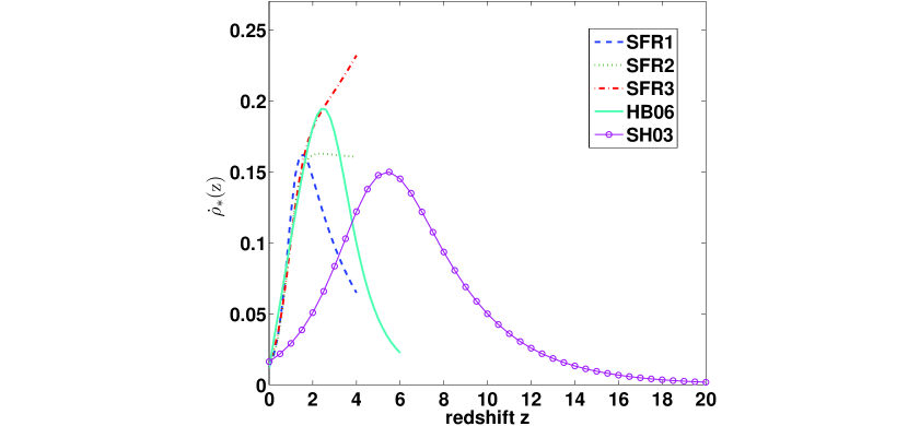
Figure 1: Evolution of the CSFR density $\dot{\rho}_{\ast}(z)$ (in $M_{\odot}\hskip 1.42262pt\rm{yr}^{-1}\hskip 1.42262pt\rm{Mpc}^{-3}$) predicted in five parameterized models (see text).

Many authors have addressed the issues of calibrating the high-z CSFR through long-duration gamma-ray bursts (GRBs) (see, e.g., Yüksel et al. 2008 and Kistler et al. 2009). Recently Wang $\&$ Dai (2009) uses latest GRBs data to constrain the CSFR up to $z=8.3$. Meanwhile there are other methods to determine the high-z CSFR, such as observations of color-selected Lyman break galaxies (LBGs) (Bouwens et al. 2008) and $Ly\alpha$ emitters (Ota et al. 2008). However, such calibrations cannot reach considerable agreements except for an overall decline at $z\geq 4$ (see Figure 1 of Yüksel et al. 2008, Kistler et al. 2009 and Wang & Dai 2009). Due to huge uncertainties and the incompleteness of data sets we will not include them here.

On the other hand, Springel & Hernquist (2003) derive the CSFR from hydrodynamic simulation of structure formation in $\Lambda$CDM cosmology. They study the history of cosmic star formation from the “dark ages”, at redshift $z=20$ to the present. The CSFR obtained in their study is broadly consistent with measurements given observational uncertainty and can be remarkably well-fitted by the following form (hereafter SH03):

$$\dot{\rho}_{\ast}(z)=\dot{\rho}_{m}\frac{\beta\exp[\alpha(z-z_{m})]}{\beta-\alpha+\alpha\cdot\exp[\beta(z-z_{m})]},$$ (3)

where $\alpha=3/5$, $\beta=14/15$, $z_{m}=5.4$ marks a break redshift and $\dot{\rho}_{m}=0.15$ $M_{\odot}\hskip 1.42262pt\rm{yr}^{-1}\hskip 1.42262pt\rm{Mpc}^{-3}$ fixes the overall normalization. It is worth mentioning that they consider a $\Lambda$CDM model with the same parameters with our assumed 737 cosmology.

In Fig. 1 we plot the CSFR predicted in the above five models as a function of redshift. SFR1, SFR2 and SFR3 show distinguishable features at $z\geq 2$. SH03 peaks at a much higher redshift, between $z=5$ and $z=6$, than observation-based models (around $z\simeq 2$). The cutoff of each curve in Fig. 1 corresponds to maximum redshifts of CSFR models: $z_{\star}=4$ for SFR1-3, $z_{\star}=6$ for HB06 and $z_{\star}=20$ for SH03. What Fig. 1 illustrates is our poor understanding about star formation history at high redshifts from astronomical observations.

Note that there are some other CSFR models, similar to or different from the five models adopt here, not included since our aim is not to make a complete survey on this issue but to phenomenologically investigate its influences on the SGWB from an ensemble of astrophysical sources. We refer readers to Calura & Matteucci (2003), Daigne et al. (2004), Bromm & Loeb (2006), Nagamine et al. (2006) and Fardal et al. (2007) for details of other studies on the determination of CSFR. In the following sections we will investigate how different CSFRs affect the rate of NS formation and spectral properties of AGWB.

3 Neutron star formation rate

Since the evolving rate of CCSNe closely tracks the star formation rate, using CSFR models presented in Section 2 we can estimate the number of NSs formed per unit time within the comoving volume out to redshift z (Ferrari et al. 1999a):

$$R_{NS}(z)=\int_{0}^{z}\dot{\rho}_{\ast}(z^{\prime})\frac{dV}{dz^{\prime}}dz^{\prime}\int_{m_{\rm{min}}}^{m_{\rm{max}}}\Phi(m)dm,$$ (4)

where $\dot{\rho}_{\ast}(z)$ is the CSFR density, $dV/dz$ is the comoving volume element, and $\Phi(m)$ is the IMF. Here we assume that each CCSN results in either a NS or a BH and take a NS progenitor mass range of $8M_{\odot}-25M_{\odot}$. In order to make comparison with Ferrari et al. (1999b) we also consider a lower upper limit for NS progenitor masses $m_{\rm{max}}=20M_{\odot}$ as indicated from core collapse simulations by Fryer (1999). However according to Belczynski & Taam (2008) the mass of NS progenitor might be greater than $40M_{\odot}$ for stars in a binary system. So we will also include a higher limit of $m_{\rm{max}}=40M_{\odot}$ for our calculations of NS formation rate (In Sigl 2006 the progenitor mass to form a NS ranges from $10M_{\odot}$ to $40M_{\odot}$).

Note that in some studies (e.g., Coward et al. 2001; de Araujo et al. 2004; Regimbau & Mandic 2008) with respect to AGWB there is an additional $(1+z)$ term in Eq.(4) dividing the CSFR to account for the time dilatation of CSFR due to cosmic expansion. Here we do not include such a term according to de Araujo & Miranda (2005) who argue that the inclusion of this additional term is inadequate.

To integrate through Eq.(4) one still needs to know the forms of $dV/dz$ and $\Phi(m)$. Following Regimbau & Mandic (2008), the comoving volume element is related to z through

$$\frac{dV}{dz}=4\pi\frac{c}{H_{0}}\frac{r(z)^{2}}{E(\Omega,z)},$$ (5)

where $H_{0}$ the Hubble constant, $E(\Omega,z)=\sqrt{\Omega_{\Lambda}+\Omega_{m}(1+z)^{3}}$ and $r(z)$ the comoving distance related to the luminosity distance by $d_{L}=r_{z}(1+z)$.

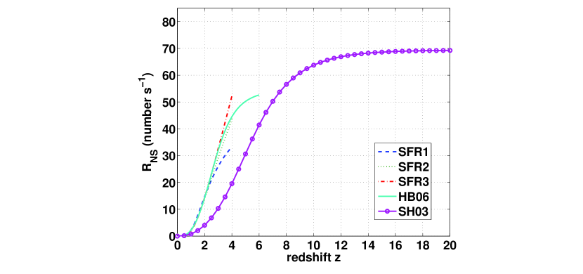
Figure 2: Evolution of the NS formation rate under different CSFR models.

We consider the standard Salpeter IMF: $\Phi(m)=Am^{-(1+x)}$ with $x=1.35$, where A is a normalization constant, obtained through the relation $\int_{m_{1}}^{m_{u}}m\Phi(m)dm=1$ with $m_{1}=0.1M_{\odot}$ and $m_{u}=125M_{\odot}$. Then we plot the NS formation rate $R_{\rm{NS}}(z)$ defined in Eq.(4) for the CSFR models presented in Section 2 with a modest value of $m_{\rm{max}}=25M_{\odot}$ in Fig. 2. Note that SFR1, SFR2 and SFR3 show quite different behaviors for $z>2.5$ and observation-based models give rise to more NS formation than SH03 up to respective redshift limits, but SH03 predicts a much higher cumulative NS formation rate for $z\geq 10$.

In Table 1 we present the total number (per unit time) of CCSN explosions leaving behind a NS out to corresponding redshift limits for the five CSFR models, and for three values of $m_{\rm{max}}$ : $20M_{\odot}$, $25M_{\odot}$ and $40M_{\odot}$. We compare the results obtained here with those in Ferrari et al. (1999b), and find a factor of $\sim 2-3$ enhancement for the total NS formation rate, which is mainly due to differences of CSFR models and cosmology terms (e.g., different forms for the comoving volume element).

Table 1: Total rate of NS formation in five CSFR models for three values of the upper limits of NS progenitor masses.

Model (redshift limit)	$m_{\rm{max}}=20M_{\odot}$	$25M_{\odot}$	$40M_{\odot}$
SFR1   ($z_{\star}=4$)	30.0	33.2	37.4
SFR2   ($z_{\star}=4$)	39.3	44.5	49.1
SFR3   ($z_{\star}=4$)	47.2	52.2	58.9
HB06   ($z_{\star}=6$)	47.5	52.6	59.3
SH03   ($z_{\star}=20$)	62.0	68.6	77.4

4 Spectral properties of the SGWB from NS r-mode instability

In this section we will evaluate the spectral properties of the stochastic background produced by an ensemble of newly born NSs with nonlinear r-mode instabilities. Initially, let us review the formalism used to characterize the AGWB.

It is useful to characterize the spectral properties of a SGWB by specifying how the energy is distributed in frequency domain. Explicitly, one introduces a dimensionless quantity, $\Omega_{\rm{GW}}$ given by:

$$\Omega_{\rm{GW}}(\nu_{\rm{obs}})=\frac{1}{\rho_{c}}\frac{d\rho_{\rm{GW}}}{d\ln\nu_{\rm{obs}}},$$ (6)

where $\rho_{\rm{GW}}$ is the GW energy density, $\nu_{\rm{obs}}$ the frequency in the observer frame and $\rho_{c}=3H_{0}^{2}/8\pi G$ is the critical energy density required to close the universe today. For a stochastic background of astrophysical origin, the energy density is given by:

$$\Omega_{\rm{GW}}(\nu_{\rm{obs}})=\frac{\nu_{\rm{obs}}}{c^{3}\rho_{c}}F_{\nu}(\nu_{\rm{obs}}),$$ (7)

where the spectral density of the flux at the observed frequency $\nu_{obs}$ is defined as

$$F_{\nu}=\int f_{\nu}(\nu_{\rm{obs}})dR,$$ (8)

where $f_{\nu}(\nu_{\rm{obs}})$ is the energy flux per unit frequency (in $\rm{erg}\cdot\rm{cm}^{-2}\cdot\rm{Hz}^{-1}$) produced by a single source and $dR$ is the differential GW event rate.

The energy flux per unit frequency $f_{\nu}(\nu_{\rm{obs}})$ can be written as follows (Carr 1980)

$$f_{\nu}(\nu_{\rm{obs}})=\frac{\pi c^{3}}{2G}h_{c}^{2},$$ (9)

where $h_{c}$ is the dimensionless amplitude produced by an event that generates a signal with observed frequency $\nu_{\rm{obs}}$.

In order to obtain the spectral properties (e.g., the values of $\Omega_{\rm{GW}}$ as a function of $\nu_{\rm{obs}}$) of the r-mode stochastic background, we have the differential rate of source formation $dR_{\rm{NS}}(z)$ through Eq.(4) and still need to know the energy flux emitted by a single source.

It has been shown that differential rotation can significantly influence the detectability of GWs emitted by a spinning-down newborn NS due to r-mode instability (Sá & Tomé 2006). Studies of mode-mode coupling in rotating stars also indicate that the maximum amplitude that r-mode can grow to is much smaller than previously estimated (Arras et al. 2003). Here we use the characteristic GW amplitude given by Sá & Tomé (2006):

$$h_{c}(\nu)=\frac{5.5\times 10^{-22}}{\sqrt{K+2}}\sqrt{\frac{\nu}{\nu_{\rm{max}}}}\left(\frac{20Mpc}{d_{L}}\right),$$ (10)

where $K$ is a constant giving the initial amount of differential rotation associated with the r-mode, and lies in the interval $-5/4\leq K\leq 10^{13}$ (see Sá & Tomé (2006) for details), $\nu=\nu_{\rm{obs}}(1+z)$ is the frequency in the source frame, $\nu_{\rm{max}}$ the maximum frequency of emitted GWs given by $2\Omega_{\rm{K}}/3\pi$ where $\Omega_{\rm{K}}=5612$ Hz is the Keplerian frequency at which the star starts shedding mass at the equator, assumed to be the initial value of the angular velocity of the star, and $d_{L}$ is the luminosity distance to the source. Note that the saturation amplitude $\alpha\propto(K+2)^{-1/2}$ (Sá & Tomé 2006), which means the GW amplitude is proportional to $\alpha$, same as those given in Bondarescu et al. (2009). In the following calculations we should keep in mind that the parameter $K$ used in this paper is equivalent to the saturation amplitude $\alpha$ of NS r-mode instability.

From the above equations we can obtain the dimensionless energy density:

$$\Omega_{\rm{GW}}(\nu_{\rm{obs}})={4\pi^{2}(1.1\times 10^{-20})^{2}\over 3H_{0}^{2}(K+2)}\frac{\nu_{\rm{obs}}^{2}}{\nu_{\rm{max}}}\times\bigg{[}\int_{z_{\rm{min}}}^{z_{\rm{max}}}\int_{m_{\rm{min}}}^{m_{\rm{max}}}\dot{\rho}_{\ast}(z)(1+z)\bigg{(}\frac{1\rm{Mpc}}{d_{L}}\bigg{)}^{2}{dV\over dz}\Phi(m)dmdz\bigg{]}.$$ (11)

Thus, by setting a value for $K$ one can calculate $\Omega_{GW}$ numerically through Eq.(11) combined with corresponding equations for CSFR, comoving volume element and IMF. Here we set $m_{\rm{min}}=8M_{\odot}$ and $m_{\rm{max}}=25M_{\odot}$, while $z_{\rm{min}}$ and $z_{\rm{max}}$ can be determined in such a way: since frequencies of emitted GWs in the source frame range from $\nu_{\rm{min}}=77-80$ Hz to $\nu_{\rm{max}}=2\Omega_{\rm{K}}/3\pi=1191$ Hz, where the minimum frequency corresponds to the final angular velocity of the star - $0.065\Omega_{\rm{K}}$ for $K=-5/4$ and $0.067\Omega_{\rm{K}}$ if $K\gg 1$, we have $\nu_{\rm{min}}/(1+z)\leq\nu_{\rm{obs}}\leq\nu_{\rm{max}}/(1+z)$, which means sources with different redshifts that produce a signal at the same frequency $\nu_{\rm{obs}}$ should meet the condition: $\nu_{\rm{min}}/\nu_{\rm{obs}}-1\leq z\leq\nu_{\rm{max}}/\nu_{\rm{obs}}-1$. Besides, we consider signals emitted at early epochs up to the present ($z\geq 0$) and take into account the maximal redshift ($z_{\ast}$) of CSFR model. Then we obtain $z_{\rm{min}}=\rm{max}(0,\nu_{\rm{min}}/\nu_{\rm{obs}}-1)$, $z_{\rm{max}}=\rm{min}(z_{\ast},\nu_{\rm{max}}/\nu_{\rm{obs}}-1)$, which is similar to that of Owen et al. (1998) where $z_{\ast}\simeq 4$ is considered to be the maximum redshift where there was significant star formation.

In Fig. 3 we plot the dimensionless energy density $\Omega_{\rm{GW}}$ calculated for the five CSFR models presented in Section 2 by setting $K$ at its minimal value: $K=-5/4$ corresponding to the smallest amount of differential rotation at the time when the r-mode instability becomes active. However, as emphasized by Sá & Tomé (2005), if $K$ is small, namely, $K\approx 0$, it is necessary to consider other nonlinear effects like mode-mode couplings in the calculation of $\alpha$, which will again limit the maximum r-mode amplitude to values much smaller than unity Arras et al. (2003). In this respect, our choice of a minimum $K$ results in an unrealistically high upper limit for r-mode background.

It is worth noting from Fig. 3 that no obvious differences are recorded for the three curves of SFR1, SFR2 and SFR3, and observation-based CSFR models give rise to stochastic backgrounds about two times stronger than that of SH03 over a broad frequency band, although SH03 leads to a much higher NS formation rate. The sharp contrast between Fig. 3 and Fig. 2 indicates that the main contribution to the GW background comes from low-redshift sources because those events happened at higher redshifts have minor influences due to the inverse squared luminosity distance dependence of the single event energy flux. For the same reason, poor observational understanding of high-z star formation history (see Fig. 1) is not severe to studies about AGWB here.

To assess the role of $z_{\ast}$ in our results, we choose SFR2 (since it remains constant for $z\geq 2$), set three values for $z_{\ast}$ ($z_{\ast}=4,10$ and $20$), and then plot the $\Omega_{\rm{GW}}$ in Fig. 4. It is surprising that the three curves exhibit almost the same pattern in the frequency range $\nu_{\rm{obs}}\geq 100$ Hz, and extending the redshift limit from 4 to 20 results in a growth of the lower-frequency background. Increasing $z_{\ast}$ will enhance the background at lower frequencies and even enable some formerly “unavailable” low-frequency signals to emerge. This low-frequency GW “tail” can be accounted for by the contribution from high-redshift sources. However if CSFR is much lower at high-z, this effect will be negligible. Thus Fig. 4 further support the conclusions from Fig. 3 and indicate that the most significant contribution to an AGWB comes from GW events occurring at redshifts $z\leq 4$.

From Eq. (11) we find that $\Omega_{\rm{GW}}$ depends on the values of $\nu_{\rm{max}}\sim\Omega_{\rm{K}}$ and $K$ ($\Omega_{\rm{GW}}\propto\frac{1}{K+2}\sim\alpha^{2}$). As suggested by Ferrari et al. (1999b), the Keplerian velocity $\Omega_{\rm{K}}$ may have a broad distribution due to different masses and radii of rotating NSs. Here we arbitrarily set $\nu_{\rm{max}}$ ranging from $1000$ Hz to $2000$ Hz. For $K$ we set $-5/4,100$ and $10^{4}$ corresponding to $\alpha=1,0.1$ and $10^{-2}$ respectively. Then we adopt HB06 as the CSFR model (below we will use only HB06) and plot $\Omega_{\rm{GW}}$ as a function of observed frequency for different values of $\alpha$ and $\nu_{\rm{max}}$ in Fig. 5. We can see a higher peak for $\Omega_{\rm{GW}}$ when we increase the maximum emitting frequency, while the r-mode background for smaller $\nu_{\rm{max}}$ is slightly enhanced at lower frequencies ($\leq 400$ Hz). On the other hand, increasing the amount of differential rotation significantly reduce the closure density and then affect the detectability of r-mode background as we will discuss later. Considering a maximum value of $10^{-2}$ for $\alpha$, a realistic estimate of r-mode background should have a energy density at most $\sim 10^{-12}$ like the lowest curve shown in Fig. 5.

Another important quantity of the AGWB is the so-called duty cycle, which classifies the stochastic backgrounds in terms of continuous background, popcorn noise and short noise (Coward & Regimbau 2006):

$$D=\int_{0}^{\infty}\bar{\tau}(1+z)dR_{\rm{NS}}(z),$$ (12)

where $\bar{\tau}$ is the average time duration of the GW emission from a single source at the source frame, which dilated to $\bar{\tau}(1+z)$ by the cosmic expansion, and $dR_{\rm{NS}}(z)$ is the differential rate of NS formation in Eq.(4). It has been suggested that differential rotation can remarkably influence the long-term spin and thermal evolution of NSs by prolonging the duration of the r-modes (Yu et al. 2009). In view of the prolonged r-mode, the spinning-down phase can last even longer than 1 yr, which indicates a duty cycle $>\sim 10^{9}$. In the next section, we will discuss the detectability of this continuous GW background.

5 Detectability

5.1 Detecting the r-mode background with a network of IFOs

We cannot reach sufficient sensitivity for detection of a SGWB with a single terrestrial IFO since the output of a detector is dominated by the noise rather than by the signal due to the stochastic background itself (Allen 1996a; Maggiore 2000). The optimal strategy to search for a SGWB is to cross correlate measurements of two or more detectors. It has been shown that after correlating signals of two detectors for a (i) isotropic, (ii) unpolarized, (iii) stationary, and (iv) Gaussian stochastic background (see Allen & Romano 1999 for discussions of these assumptions), the optimal SNR during an integration time T (here we assume $T=3\rm{yr}\simeq 10^{8}$ s) is given by an integral over frequency $f$:

$$\left({S\over N}\right)^{2}={9H_{0}^{4}\over 50\pi^{4}}T\int_{0}^{\infty}df\>{\gamma^{2}(f)\Omega_{\rm{GW}}^{2}(f)\over f^{6}P_{1}(f)P_{2}(f)}\ ,$$ (13)

where $P_{1}(f)$ and $P_{2}(f)$ are the power spectral noise densities of the two detectors and $\gamma(f)$ is the so-called overlap reduction function, first calculated by Flanagan (1993). This is a dimensionless function of frequency and determined by the relative locations and orientations of two detectors. For $\gamma(f)$, we refer readers to Flanagan (1993), Allen & Romano (1999), Maggiore (2000) for more details.

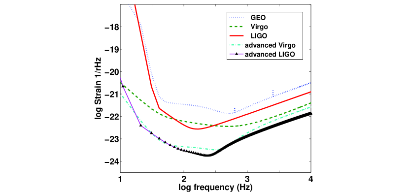
Figure 6: The designed noise power spectrum of the GEO, Virgo, initial LIGO, advanced Virgo and advanced LIGO. Data are taken from Lazzarini et al. 1996, Punturo 2004, http://www.aei.mpg.de/jrsmith/geocurves.html, http://wwwcascina.virgo.infn.it/advirgo/ and https://dcc.ligo.org/cgi-bin/DocDB/ShowDocument?docid=2974.

To assess the detectability of the r-mode background, we will calculate the SNRs for several pairs of detectors for $\Omega_{\rm{GW}}$ computed with HB06 CSFR model, $K=-5/4$ and $\nu_{\rm{max}}=1191$ Hz (unless otherwise stated we use these parameters in Section 5). Here we consider the four IFOs which are in routine operations - LIGOH (4km), LIGOL (4km), Virgo (3km) and GEO (600m), as well as the second generation detectors - advanced LIGO and advanced Virgo. Design sensitivity curves of these detectors are shown in Fig. 6. It is worth mentioning that the first-generation GW interferometric detectors have taken data at, or close to, their design sensitivities (Fairhurst et al 2009). In particular, the design sensitivity curve for initial LIGO was almost attained by its S5 run. In the following calculations we will use real $\gamma(f)$ for different pairs of IFOs unless otherwise stated.

Two approaches of combining 2N detectors to improve the detection ability to the SGWB are proposed in Allen & Romano (1999): (i) correlating the outputs of a pair of detectors, then combining multiple pairs (combining pairs, “c-p”), and (ii) directly combining the outputs of 2N detectors (directly combining, “d-c”). For the first approach, the squared SNR is given by:

$$\left({S\over N}\right)^{2}_{optI}=\sum_{pair}\left({S\over N}\right)^{2}_{pair},$$ (14)

and for the second one:

$$\left({S\over N}\right)^{2}_{op\,tII}\approx{}^{(12)}\left({S\over N}\right)^{2}\ {}^{(34)}\left({S\over N}\right)^{2}\cdots{}^{(2N-1,2N)}\left({S\over N}\right)^{2}+\hbox{{\rm\ all possible permutations}}\ .$$ (15)

Table 2: Concerning the detection of the r-mode background, we present the SNRs calculated for multiple detector pairs of LIGOH (H), LIGOL (L), Virgo (V) and GEO (G) and two approaches of combining the four IFOs - combining pairs (c-p) and directly combining (d-c). Case 1 corresponds to first-generation detectors and Case 2 adopts sensitivities of advanced LIGO and advanced Virgo, while G refers to an assumed interferometer with the same sensitivity as advanced Virgo at the GEO site.

Case	H-L	L-V	H-V	V-G
1	$1.8\times 10^{-3}$	$1.0\times 10^{-3}$	$8.5\times 10^{-4}$	$2.6\times 10^{-4}$
2	0.40	0.21	0.17	0.25
Case	L-G	H-G	c-p	d-c
1	$1.4\times 10^{-4}$	$9.7\times 10^{-5}$	$2.3\times 10^{-3}$	$5.0\times 10^{-7}$
2	0.16	0.11	0.58	0.11

We show in Table 2 the SNRs calculated for different pairs of LIGOH, LIGOL, Virgo and GEO, and for two combinations of these four IFOs. We consider here two cases representing two real networks of first/second generation IFOs: Case 1 is for these four IFOs with design sensitivities; Case 2 consists of two advanced LIGO detectors and two advanced Virgo detectors both with proposed sensitivities. Note that SNRs in Table 2 are lower than unity even for pairs of advanced detectors. The most promising one ($SNR=0.58$) comes from combining pairs of four advanced IFOs. If we assume an optimized value of unity for $\gamma(f)$, which is only possible for co-located GW detectors Fotopoulos & LSC (2008), the SNR is $11.0$ and $4.1$ for a pair of advanced LIGO and advanced Virgo IFOs respectively. We note that by considering new detectors with comparable sensitivities to advanced LIGO, such as LCGT in Japan (Kuroda et al. 1999) and AIGO in Australia (Blair et al. 2008), it could be possible to reach a higher, but still not significant SNR with a network of second-generation IFOs.

In order to obtain some detectable parameter space we need at least one order of magnitude higher SNRs than those in Case 2 of Table 2. Then we reduce the noise power spectral densities of advanced LIGO and advanced Virgo by a factor of 10 by hand, and investigate the role of differential rotation ($K$) and maximum emitting frequency ($\nu_{\rm{max}}$) in the detectability of the r-mode background. We are motivated here by the fact that third-generation detectors like ET can reach a sensitivity roughly an order of magnitude better than that of advanced LIGO (Hild et al. 2008).

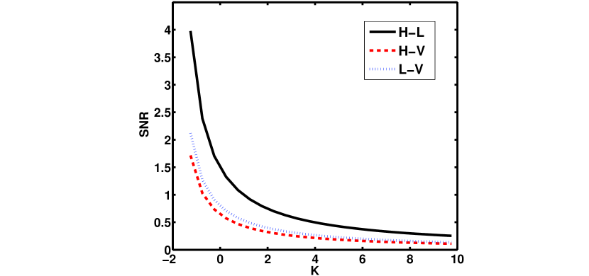
Figure 7: SNR as a function of $K$ for H-L, H-V and L-V pairs when we set $\nu_{\rm{max}}=1191$ Hz. We assume a factor of 10 folds improvement in sensitivity for advanced LIGO and advanced Virgo detectors.

In Fig. 7 we plot the SNR as a function of $K$ for H-L, H-V and L-V pairs. As a natural result from Fig. 5, the detectability of SGWB from r-mode instability is drastically reduced to 0 as $K$ approaching 10. The higher SNR of H-L pair reflects the lower noise level of advanced LIGO. Due to similarity of the overlap reduction functions (see Fig. 2 of Fan & Zhu 2008) no significant difference is shown between L-V and H-V pairs.

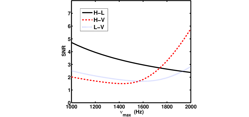
Figure 8: Same as Fig. 7, SNR as a function of $\nu_{\rm{max}}$ for H-L, H-V and L-V pairs when we set $K=-5/4$.

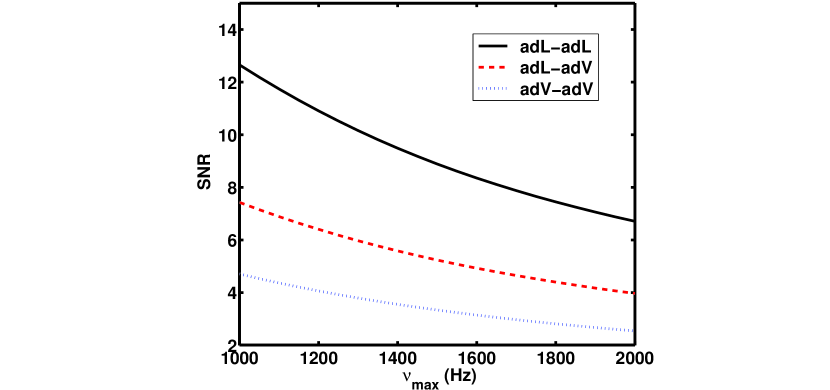
Figure 9: SNR as a function of $\nu_{\rm{max}}$ assuming $\gamma(f)=1$ for two advanced LIGO (adL) detectors, two advanced Virgo (adV) detectors and the combination between them (here no improvement of sensitivity is assumed).

Fig. 8 shows the SNR evolution with $\nu_{\rm{max}}$ for H-L, H-V and L-V pairs. In contrast to Fig. 5, in which a higher peak value of $\Omega_{\rm{GW}}$ was obtained for larger $\nu_{\rm{max}}$, there are no identical features for SNR evolutions here. For H-L pair, we note that SNR varies inversely as the increase of $\nu_{\rm{max}}$. This can be explained that the low-frequency GW background is enhanced for smaller $\nu_{\rm{max}}$ while the growth of high-frequency background due to larger $\nu_{\rm{max}}$ is suppressed by the $1/f^{6}$ term in Eq. (13). On the other hand, we can reach higher SNRs for H-V and L-V pairs for larger $\nu_{\rm{max}}$ ($\geq 1600$ Hz). This unique feature can be attributed to particular evolving behaviors of $\gamma(f)$ for the two pairs (see again Fig. 2 of Fan & Zhu 2008 and we will find that $\gamma(f)$ is extremely close to zero at high frequencies for H-L, while it still fluctuates above and below zero up to $1000$ Hz for H-V and L-V pairs). This is strongly supported by three curves in Fig. 9, where we plot the SNR as a function of $\nu_{\rm{max}}$ by assuming $\gamma(f)=1$ , show exactly the same evolving pattern as the curve of H-L in Fig. 8.

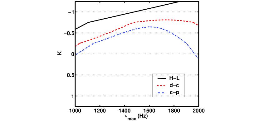
Figure 10: The region of parameter space for which SGWB produced from an ensemble of NSs with r-mode instability is detectable by H-L pair (here an order of magnitude improvement for advanced LIGO sensitivity is assumed), the approach of directly combining (labeled “d-c”) four third-generation detectors (an order of magnitude improvement in detector sensitivities for Case 2 in Table 2 is assumed) and the approach of combining multiple pairs of detectors (labeled “c-p”). With $10\%$ false alarm and $90\%$ detection rate, the region above the curves shows the detectable parameter space.

For a detection rate $90\%$ and a false alarm rate $10\%$, the total optimal SNR threshold should be 2.56. In order to evaluate the promise of detecting the r-mode background we present in Fig. 10 the regions in the ($\nu_{\rm{max}},K$) plane where SNR could be higher than 2.56 for multiple detector pairs. It is shown that the detectable parameter space is quite limited even for a real network of third-generation IFOs. In particular, a strong constraint for ($K<0$ or equivalently $\alpha\sim 1$) is obtained. Meanwhile we find that two approaches of combining multiple IFOs can effectively improve the detection ability as compared to H-L pair, and “c-p” method performs better than “d-c” approach in terms of detecting the r-mode background.

5.2 The detection prospects of future detectors

In this section we discuss further the detection prospects of a SGWB from NS r-mode instability by networks of third generation instruments.

Fig. 10 indicates that only when the initial amount of differential rotation is near its minimum value ($K\simeq 0$), the r-mode background could be detectable by a real network of third-generation GW detectors. However, as emphasized by Sá & Tomé (2005), if $K$ is near its minimum value, other nonlinear effects like mode-mode couplings should be included in the calculation of saturation amplitude $\alpha$. Still in this case, $\alpha$ will be limited to values much smaller than unity Arras et al. (2003). In this respect the physically reasonable values of parameter $K$ introduced in Sá & Tomé (2005) should be larger than $10^{4}$ in order to be consistent with a maximum saturation amplitude $\alpha\leq 10^{-2}$ Lin & Suen (2006).

It seems most probable that the r-mode background is not going to be detectable. Given the relation $SNR\sim\Omega_{\rm{GW}}\sim\alpha^{2}$, a $10^{-2}$ saturation amplitude (compared with a value of order unity) will reduce the SNR by 4 orders of magnitude for any measurements of SGWB from NS r-mode instability. In particular, to reach the same SNR requires 10000 times improvements in sensitivities of two detectors.

If we leave the small $\alpha$ issue (the dominant aspect) aside, it is still quite pessimistic to detect the r-mode background as seen from Table 2 and Fig. 10. This is due to the following facts: 1) the closure density of this background peaks at much higher frequencies than the most sensitive frequency band of ground-based detectors; 2) the minimum frequency of r-mode GW signal $\nu_{\rm{min}}=80$ Hz just misses the frequency band (1-60 Hz) where the overlap reduction functions of real detector pairs are significant; 3) we should not forget that we assumed all NSs are born with angular velocities near their maximal value $\Omega_{\rm{K}}$. This is not necessarily always the case since it would make more sense to consider some fraction of NSs are born with rapid spins (Owen et al. 1998). Actually it has been suggested that most NSs are born with very small rotation rates Spruit & Phinney (1998). Current population synthesis studies favor spin periods of NSs at birth in the range from tens to hundreds of milliseconds Ott et al. 2006 ; Perna et al. (2008).

Realistic overlap reduction functions are adopted here for multiple ground-based IFOs. Recall that two co-located advanced LIGO detectors ($\gamma(f)=1$, SNR=11) perform even better than combining four IFOs with 10-fold better sensitivities (SNR=5.8). With this in mind we also evaluate the detectability of r-mode background with ET, assuming two detectors located in Cascina, of triangular shape ($60^{\circ}$ between the two arms) and separated by an angle of $120^{\circ}$ Howell et al. (2010). The $\gamma(f)$ benefits a lot from this configuration, nearly linearly decreasing from $-0.372$ at 1000 Hz to $-0.375$ at 1 Hz. We adopt the ET-B sensitivity from Hild et al. (2008). For 3-year integration, a SNR of 2.56 requires $K\leq\sim 150$ corresponding to $\alpha\sim 0.1$.

Then we convert the constrains on $K$ or $\alpha$ to absolute numbers: the total emitted GW energy associated with NS r-mode instability that enable the stochastic background to be detectable by future detectors. The energy flux of single event can also be written as:

$$f(\nu_{\rm{obs}},z)=\frac{1}{4\pi d_{L}(z)^{2}}\frac{dE_{\rm{GW}}}{d\nu}(1+z),$$ (16)

where $dE_{\rm{GW}}/{d\nu}$ is the gravitational spectral energy. Combined with Eq.(9) and Eq.(10) we can obtain the spectral energy density and thus the total GW energy emitted by individual sources that contribute to this background. We give the results (required energy level in order to obtain a SNR of 2.56 by 3-year integration) as follows (in $M_{\odot}c^{2}$): i) $1.8\times 10^{-3}$ for a real network of “third-generation” IFOs; ii) $9.4\times 10^{-4}$ for two co-located advanced LIGO detectors; iii) $2\times 10^{-5}$ for two detectors with ET-B sensitivity.

6 Conclusions

We revisit the possibility and detectability of a SGWB produced by a cosmological population of young NSs with an r-mode instabilities. Source formation rate is accounted for by using a set of CSFR models, both observational and simulated. Our results show that the resultant GW background is insensitive to the choice of CSFR models (although they predict quite different NS formation rates), but dependent on the evolving behavior of CSFR at low redshifts ($z\leq 2$). This is in good agreement with that in Howell et al. (2004). But here we further investigate the effect of the maximal redshift of CSFR models on the AGWB and find that high-redshift ($z>4$) sources could form a GW “tail” in the low-frequency side ($\leq 30$ Hz, this number depends on particular source spectrum and thus only applies to r-mode background) and has no effect on the high-frequency background. Such an effect will be negligible if high-z CSFR is much smaller. Our Fig. 3 and Fig. 4 indicate that the most significant contribution to the GW background of astrophysical origin comes from GW events occurring at redshifts $z\leq 4$.

The characteristic GW amplitude parametrized with the initial amount of differential rotation ($K$) during r-mode evolution is adopted as the average GW signal for individual sources. While a minimum $K$ corresponding to a saturation mode amplitude $\alpha\sim 1$ is assumed, the energy density $\Omega_{\rm{GW}}$ has a maximum amplitude at around $3\times 10^{-8}$, agreeing well with those of Owen et al. (1998) and Ferrari et al. (1999b). However since we know that the maximum amplitude $\alpha$ that r-mode can grow to is at most $10^{-3}-10^{-2}$. This means the physically reasonable values of parameter $K$ is at least $10^{4}$. Consequently a realistic estimate of $\Omega_{\rm{GW}}$ for r-mode background should be at most $\sim 10^{-12}$.

We further consider multiple IFOs, including the first-generation ones that are in routine operations and upgraded counterparts, for the detection of r-mode background. We also illustrate how a network of ground-based IFOs could improve the detection ability to this GW background. Since the detectability is dominated by the square of saturation amplitude ($SNR\propto\alpha^{2}$), it is likely that the r-mode background will not be detectable for any future detectors. Still we give the constraints on the total emitted GW energy associated with this mechanism to enable a detection with $90\%$ detection rate ($SNR=2.56$) by 3-year cross correlation as: $\sim 10^{-3}\hskip 2.84526ptM_{\odot}c^{2}$ for two co-located advanced LIGO detectors and $2\times 10^{-5}$ for two IFOs with ET sensitivity. Considering the relatively certain NS formation rate, these constraints might be applicable to alternative emission mechanisms associated with NS oscillations and instabilities. This requires further investigation. The requirement on GW energy level could be lower if more signals are emitted near the most sensitive frequency band of ground-based detectors ($\sim 40-200$ Hz). Through reasonable assumptions of average source spectra, the lowest detectable (in terms of stochastic background) GW energy for individual source will be $10^{-7}\hskip 2.84526ptM_{\odot}c^{2}$ for third generation detectors like ET Zhu et al. (2010). Overall, for the detection of SGWB from NS instabilities, more efficient emitters are required (see, e.g., Andersson et al. 2010 for reviews of GW emission from NSs and Kastaun et al. 2010 for details of a possible more efficient mechanism - f-mode).

While the SGWB from NS r-mode instability is difficult to detect, the associated GW signal is still detectable in terms of single events Owen 2010 , although this possibility also depends strongly on the saturation amplitude. For instance, initially it was believed that GWs from r-mode instability in a newborn NS could be detected by advanced LIGO out to a distance of 20 Mpc Owen & Lindblom (2002). However even for the most optimistic case in Bondarescu et al. (2009), the detectable distance for advanced LIGO is only 1 Mpc. The LIGO Scientific Collaboration and Virgo Collaboration have already performed many searches for periodic GWs from rapidly rotating NSs including the first search targeting the youngest known NS - Cassiopeia A Abadie et al. (2010). Although no GWs have been detected, direct upper limits on GW emission from known pulsars like the Crab pulsar have beaten down the indirect spin-down limits Abbott et al. (2008).

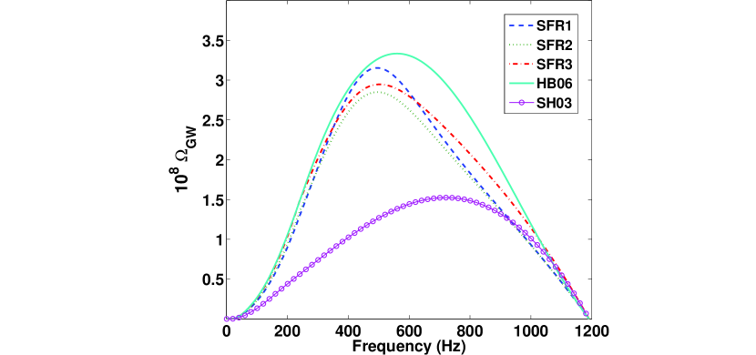
Figure 3: The dimensionless energy density $\Omega_{\rm{GW}}$ as a function of observed frequency $\nu_{\rm{obs}}$, calculated for five CSFR models and by setting $K=-5/4$, $\nu_{\rm{max}}=1191$ Hz.

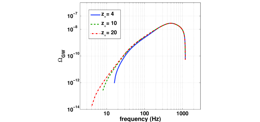
Figure 4: $\Omega_{\rm{GW}}$ as a function of observed frequency $\nu_{\rm{obs}}$, calculated for SFR2 model with three different values of maximum redshift $z_{\ast}$ and for other parameters same as Fig. 3.

Figure 5: $\Omega_{\rm{GW}}$ as a function of $\nu_{\rm{obs}}$, calculated for different values of ($\alpha$, $\nu_{\rm{obs}}$).

References

- Abadie et al. (2010) Abadie J. et al., 2010, arXiv:1006.2535
- Abbott et al. (2008) Abbott B. et al., 2008, ApJ, 683, L45
- Abbott et al. (2009) Abbott, B., et al. 2009, Nature, 460, 990
- Abramovici et al. (1992) Abramovici, A., et al. 1992, Science, 256, 325; http://www.ligo.org
- (5) Allen, B. 1996a, Lectures at Les Houches School, arXiv:gr-qc/9604033
- (6) Allen, B. 1996b, arXiv:gr-qc/9607075
- Allen & Romano (1999) Allen, B., & Romano, J. D. 1999, Phys. Rev. D, 59, 102001
- Andersson (1998) Andersson, N. 1998, ApJ, 502, 708
- Andersson (2003) Andersson, N. 2003, Classical Quantum Gravity, 20, 105
- Andersson et al. (1999) Andersson, N., Kokkotas, K., & Schutz, B. F. 1999, ApJ, 510, 846,
- Andersson & Kokkotas (2001) Andersson, N., Kokkotas K.D. 2001, International Journal of Modern Physics D, 10, 381
- Andersson et al. (2010) Andersson, N., et al. 2010, General Relativity and Gravitation, 156; arXiv:0912.0384
- Ando et al. (2001) Ando, M., et al. [TAMA Collaboration] 2001, Phys. Rev. Lett., 86, 3950; http://tamago.mtk.nao.ac.jp/
- Arras et al. (2003) Arras, P., Flanagan, E. E., Morsink, S. M., Schenk, A. K., Teukolsky, S. A., & Wasserman, I. 2003, ApJ, 591, 1129
- Baldry & Glazebrook (2003) Baldry I. K., Glazebrook K., 2003, ApJ, 593, 258
- Belczynski & Taam (2008) Belczynski, K., & Taam, R. E. 2008, ApJ, 685, 400
- Blain et al. (1999) Blain, A. W., Kneib, J. P., Ivison, R. J., & Smail, I. 1999, ApJ, 512, L87
- Blair & Ju (1996) Blair, D., Ju, L. 1996, MNRAS, 283, 648
- Blair et al. (2008) Blair, D. G., et al. 2008, Journal of Physics Conference Series, 122, 012001; http://www.aigo.org.au/
- (20) Bondarescu, R., Teukolsky, S. A., & Wasserman, I. 2009, Phys. Rev. D, 79, 104003
- Bouwens et al. (2008) Bouwens, R. J., et al. 2008, ApJ, 686, 230
- Brink et al. (2004) Brink, J., Teukolsky, S. A., & Wasserman, I. 2004, Phys. Rev. D, 70, 121501
- Bromm (2005) Bromm, V., & Loeb, A. 2006, ApJ, 642, 382
- Buonanno (2003) Buonanno, A. 2003, TASI Lectures on Gravitational Waves from the Early Universe, arXiv:gr-qc/0303085
- Buonanno et al. (2005) Buonanno, A., Sigl, G., Raffelt, G. G., Janka, H. T., & Müller, E. 2005, Phys. Rev. D, 72, 084001
- Calura & Matteucci (2003) Calura, F., & Matteucci, F. 2003, ApJ, 596, 734
- Calzetti (2008) Calzetti, D. 2008, ASP Conference Series, 390, 121; arXiv: 0707.0467
- Caron et al. (1997) Caron, B., et al. 1997, Classical Quantum Gravity, 14, 1461; http://www.virgo.infn.it
- Carr (1980) Carr, B. J. 1980, A&A, 89, 6
- Cella et al. (2007) Cella, G., et al. 2007, Classical Quantum Gravity, 24, 639
- Coward et al. (2001) Coward, D. M., Burman, R. R., & Blair, D. G. 2001, MNRAS, 324, 1015
- Coward & Regimbau (2006) Coward, D. M., & Regimbau, T. 2006, New Astron. Rev., 50, 461
- Daigne et al. (2004) Daigne, F., Olive, K. A., Vangioni-Flam, E., Silk, J., & Audouze, J. 2004, ApJ, 617, 693
- de Araujo & Marranghello (2009) de Araujo, J. C. N., & Marranghello, G. F. 2009, General Relativity and Gravitation, 41, 1389
- de Araujo & Miranda (2005) de Araujo, J. C. N., & Miranda, O. D. 2005, Phys. Rev. D, 71, 127503
- de Araujo et al. (2004) de Araujo, J. C. N., Miranda, O. D., & Aguiar, O. D. 2004, MNRAS, 348, 1373
- Fairhurst et al. (2009) Fairhurst, S., et al. 2009, arXiv: 0908.4006
- Fan & Zhu (2008) Fan, X.-L., & Zhu, Z.-H. 2008, Phys. Lett. B, 663, 17
- Fardal et al. (2007) Fardal, M., Katz, N., Weinberg, D., & Dave, R. 2007, MNRAS, 379, 985
- Farmer & Phinney (2002) Farmer, A. J., & Phinney, E. S. 2002, MNRAS, 346, 1197
- (41) Ferrari, V., Matarrese, S., & Schneider, R. 1999a, MNRAS, 303, 247
- (42) Ferrari, V., Matarrese, S., & Schneider, R. 1999b, MNRAS, 303, 258
- Finn et al. (2009) Finn, L. S., Larson, S. L., & Romano, J. D. 2009, Phys. Rev. D, 79, 062003
- Flanagan (1993) Flanagan, E. 1993, Phys. Rev. D, 48, 2389
- Fotopoulos & LSC (2008) Fotopoulos, N. V., & the LIGO Scientific Collaboration 2008, Journal of Physics Conference Series, 122, 012032
- Friedman & Morsink (1998) Friedman, J. L., & Morsink, S. M. 1998, ApJ, 502, 714
- Fryer (1999) Fryer, C. 1999, ApJ, 522, 413
- Hild et al. (2008) Hild, S., Chelkowski, S., & Freise, A. 2008, arXiv: 0810.0604
- Ho & Lai (2000) Ho, W. C. G., & Lai, D. 2000, ApJ, 543, 386
- Hopkins (2004) Hopkins, A. M. 2004, ApJ, 615, 209
- Hopkins & Beacom (2006) Hopkins, A. M., & Beacom, J. F. 2006, ApJ, 651, 142
- Howell et al. (2004) Howell, E., Coward, D., Burman, R., Blair, D., & Gilmore, J. 2004, MNRAS, 351, 1237
- Howell et al. (2010) Howell, E., Regimbau, T., Corsi, A., Coward, D., & Burman, R. 2010, MNRAS, accepted (arXiv:1008.3941)
- Kastaun et al. (2010) Kastaun, W., Willburger, B., & Kokkotas, K. D. 2010, arXiv:1006.3885
- Kistler et al. (2009) Kistler, M. D., et al. 2009, ApJ, 705, L104
- Komatsu et al. (2009) Komatsu, E., et al. 2009, ApJS, 180, 330
- Kuroda et al. (1999) Kuroda, K., et al. 1999, International Journal of Modern Physics D, 8, 557; http://gw.icrr.u-tokyo.ac.jp/lcgt/
- Lazzarini et al. (1996) Lazzarini, A., et al. 1996, LIGO Science Requirement Documents, LIGO E950018-02 and http://www.ligo.caltech.edu/lazz/distribution/LSC_Data/
- Lin & Suen (2006) Lin, L.-M., & Suen, W.-M. 2006, MNRAS, 370, 1295
- (60) Lindblom, L., & Owen, B. J. 2002, Phys. Rev. D, 65, 063006
- Lindblom et al. (1998) Lindblom, L., Owen, B. J., & Morsink, S. M. 1998, Phys. Rev. Lett., 80, 4843
- Lindblom et al. (2000) Lindblom, L., Owen, B. J., & Ushomirsky, G. 2000, Phys. Rev. D, 62, 084030
- Lindblom et al. (2001) Lindblom, L., Tohline, J. E., & Vallisneri, M. 2001, Phys. Rev. Lett. 86, 1152
- Lück et al. (1997) Lück, H., et al. 1997, Classical Quantum Gravity, 14, 1471; http://www.geo600.uni-hannover.de
- Madau (1998) Madau, P. 1998, in The Young Universe: Galaxy Formation and Evolution at Intermediate and High Redshift, ed. D’Odorico S., Fontana A., Giallongo E., ASP Conference Series Vol. 148, 289
- Madau et al. (1996) Madau, P., Ferguson, H. C., Dickinson, M. E., Giavalisco, M., Steidel, C. C., & Fruchter, A. 1996, MNRAS, 283, 1388
- Madau & Pozzetti (2000) Madau, P., & Pozzetti, L. 2000, MNRAS, 312, L9
- Maggiore (2000) Maggiore, M. 2000, Phys. Rep., 331, 283
- Marassi et al. (2009) Marassi, S., Schneider, R., & Ferrari, V. 2009, MNRAS, 398, 293
- Morsink (2002) Morsink, S. M. 2002, ApJ, 571, 435
- Nagamine et al. (2006) Nagamine, K., Ostriker, J., Fukugita, M., & Cen, R. 2006, ApJ, 653, 881
- Ota et al. (2008) Ota, K., et al. 2008, ApJ, 677, 12
- (73) Ott, C. D., Burrows, A., Thompson, T. A., Livne, E., & Walder, R. 2006, ApJS, 164, 130
- (74) Owen, B. J. 2010, arXiv:1006.1994
- Owen & Lindblom (2002) Owen, B. J., & Lindblom, L. 2002, Classical Quantum Gravity, 19, 1247
- Owen et al (1998) Owen, B. J., Lindblom, L., Cutler, C., Schutz, B. F., Vecchio, A., & Andersson, N. 1998, Phys. Rev. D, 58, 084020
- Pereira & Miranda (2009) Pereira, E. S., & Miranda, O. D. 2009, MNRAS, 401, 1924
- Perna et al. (2008) Perna, R., Soria, R., Pooley, D., & Stella, L. 2008, MNRAS, 384, 1638
- Porciani & Madau (2001) Porciani, C., & Madau, P. 2001, ApJ, 548, 522
- Punturo (2004) Punturo, M. 2004, Virgo note VIR-NOT-PER-1390-51, Issue 10. Digital format from http://www.virgo.infn.it/senscurve/
- Regimbau & Chauvineau (2007) Regimbau, T., & Chauvineau, B. 2007, Classical Quantum Gravity, 24 627
- (82) Regimbau, T., & de Freitas Pacheco, J. A. 2006a, ApJ, 642, 455
- (83) Regimbau, T., & de Freitas Pacheco, J. A. 2006b, A&A, 447, 1
- Regimbau & Mandic (2008) Regimbau, T., & Mandic, V. 2008, Classical Quantum Gravity, 25, 184018
- (85) Rezzolla, L., Lamb, F. K., Marković, D., & Shapiro, S. L. 2001a, Phys. Rev. D, 64, 104013
- (86) Rezzolla, L., Lamb, F. K., Marković, D., & Shapiro, S. L. 2001b, Phys. Rev. D, 64, 104014
- Rezzolla et al. (2000) Rezzolla, L., Lamb, F. K., & Shapiro, S. L. 2000, ApJ, 531, L139
- Sá (2004) Sá, P. M. 2004, Phys. Rev. D, 69, 084001
- Sá & Tomé (2005) Sá, P. M., & Tomé, B. 2005, Phys. Rev. D, 71, 044007
- Sá & Tomé (2006) Sá, P. M., & Tomé, B. 2006, Phys. Rev. D, 74, 044011
- Sandick et al. (2006) Sandick, P., Olive, K. A., Daigne, F., & Vangioni, E. 2006, Phys. Rev. D, 73, 104024
- Schenk et al. (2002) Schenk, A. K., Arras, P., Flanagan, É. É., Teukolsky, S. A., & Wasserman, I. 2002, Phys. Rev. D, 65, 024001
- (93) Schneider, R., Ferrari, V., & Matarrese, S. 2000, Nuclear Physics B Proceedings Supplements, 80, 722
- Schneider et al. (2001) Schneider, R., Ferrari, V., Matarrese, S., & Potergies Zwart, S. F. 2001, MNRAS, 324, 797
- Sigl (2006) Sigl, G. 2006, JCAP, 4, 2
- Springel & Hernquist (2003) Springel, V., & Hernquist, L. 2003, MNRAS, 339, 312
- Spruit & Phinney (1998) Spruit, H., & Phinney, E. S. 1998, Nature, 393, 139
- Steidel et al. (1999) Steidel, C. C., Adelberger, K. L., Giavalisco, M., Dickinson, M., & Pettini, M. 1999, ApJ, 519, 1
- Stergioulas & Font (2001) Stergioulas, N., & Font, J. A. , 2001, Phys. Rev. Lett. 86, 1148
- Suwa et al. (2007) Suwa, Y., Takiwaki, T., Kotake, K., & Sato, K. 2007, ApJ, 665, L43
- Wang & Dai (2009) Wang, F.-Y., & Dai, Z.-G. 2009, MNRAS, 400, L10
- Wilkins et al. (2008) Wilkins, S. M., Trentham, N., & Hopkins, A. 2008, MNRAS, 385, 687
- Yu et al. (2009) Yu, Y.-W., Cao, X.-F., & Zheng, X.-P. 2009, Research in Astronomy and Astrophysics, 9, 1024
- Yüksel et al. (2008) Yüksel, H., et al. 2008, ApJ, 683, L5
- Zhu et al. (2010) Zhu, X.-J., Howell, E., & Blair, D. 2010, arXiv:1008.0472