Electromagnetic production of hypernuclei.

Abstract

A formalism for the electromagnetic production of hypernuclei is developed where the cross section is written as a contraction between a leptonic tensor and a hadronic tensor. The hadronic tensor is written in a model-independent way by expanding it in terms of a set of five nuclear structure functions. These structure functions are calculated by assuming that the virtual photon interacts with only one bound nucleon. We use the most recent model for the elementary current operator which gives a good description of the experimental data for the corresponding elementary process. The bound state wave functions for the bound nucleon and hyperon are calculated within a relativistic mean-field model. We calculate the unpolarized triple differential cross section for the hypernuclear production process $e+{{}^{12}{\rm C}}\,\,\longrightarrow\,\,e+K^{+}+{{}^{12}_{~{}\Lambda}}{\rm B}$ as a function of the kaon scattering angle. The nuclear structure functions are calculated within a particle-hole model. The cross section displays a characteristic form of being large for small values of the kaon scattering angle with a smooth fall-off to zero with increasing angle. The shape of the cross section is essentially determined by the nuclear structure functions. In addition, it is found that for the unpolarized triple differential cross section one structure function is negligible over the entire range of the kaon scattering angle.
Keywords: Hypernuclear; Relativistic Mean Field Models; Structure Functions; Strangeness Production

I Introduction

The study of strange particles and hypernuclei remains an area of intense theoretical and experimental activity. Hypernuclei represent an exotic state of matter since they contain particles with quantum numbers such as strangeness which are not associated with ordinary nuclear matter. Whereas the nucleon-nucleon interaction is very well-known from elastic scattering data, our knowledge of the hyperon-nucleon, and hyperon-hyperon interactions is still relatively incomplete. A major goal of nuclear physics should also be a unified understanding of baryon-baryon interactions. Studies of hypernuclei are also important since they can give us insight into the role of strangeness in the stellar environment. A free $\Lambda$ particle is unstable and will primarily decay via the weak interaction to a nucleon-pion system. However, a $\Lambda$ in the nuclear medium will interact strongly with the other nucleons, hence forming a hypernucleus. The $\Lambda$ is unaffected by the Pauli exclusion principle and can therefore occupy any one of the states already filled by the nucleons. In a one-boson-exchange picture the zero isospin of the $\Lambda$ forbids the exchange of isovector mesons such as a pion or the rho meson with a nucleon, and therefore leads to a lack of strong tensor components in the $\Lambda N$ interaction. Consequently the $\Lambda N$ interaction is much weaker than the $NN$ interaction, and the $\Lambda$ in the nucleus does not lead to a major disruption of the shell structure Gibson (1995). Hypernuclei therefore provide remarkable experimental evidence for the shell-model of nuclear structure.

A wealth of experimental data on hypernuclei have been accumulated by making use of hadronic probes Gibson (1995). These include the strangeness exchange reaction

$$K^{-}\,(s\bar{u}\,)+n\,(uud\,) \longrightarrow \Lambda\,(uds\,)+\pi^{-}\,(d\bar{u}\,)$$ (1)

and the associate production process

$$\pi^{+}\,(u\bar{d}\,)+n\,(udd\,) \longrightarrow \Lambda\,(uds\,)+K^{+}\,(u\bar{s}\,).$$ (2)

An alternative production mechanism is through the use of real or virtual photons, i.e.,

$$\gamma+p\,(uud\,) \longrightarrow K^{+}\,(u\bar{s}\,)+\Lambda\,(uds\,).$$ (3)

Hyperon production via the electromagnetic interaction requires the production of a strange quark/anti-quark pair. The large momentum transfer for associate production decreases the sticking probability of the $\Lambda$, and consequently the probability for obtaining a bound hypernuclear system in the final state Hinton (2000). Since the production of the reaction particles are limited to the very forward angles, it is necessary to detect the electron and the kaon in coincidence Hungerford (2001).

However, electron beams offer a number of distinct advantages. Indeed, with the advent of Jlab, our understanding of the role of the electromagnetic production process has greatly increased. The precision of the electron beam, as well as good spatial and energy resolution make up for the small $(e,e^{\prime},K^{+})$ cross section relative to hadronic production mechanisms Hinton (2000). The $(e,e^{\prime},K^{+})$ reaction converts a proton in a target nucleus, and populates proton-hole $\Lambda$-particle states. This reaction therefore produces neutron-rich $\Lambda$ hypernuclei. Electroproduction excites both natural and unnatural parity states with comparable strength Cohen (1985). Both the photon and the $K^{+}$ interacts relatively weakly with the nucleus and therefore the $(e,e^{\prime}K^{+})$ reaction is not confined to the nuclear surface, hence hypernuclear states can be studied with a deeply-bound hyperon. In heavier nuclei the behavior of a $\Lambda$ in nuclear matter may be studied. The transition operator has a spin-part, hence one can also probe spin-flip states. The electron beam can be polarized, whereas no polarized $K^{-}$ (or $\pi^{+}$) beams exist Cohen (1985).

The study of baryonic resonances is an important field in hadron phenomenology. Theoretical work to determine the excitation spectrum of nucleons has been done mainly within the quark model framework. However, these models predict a much richer spectrum than what has been observed with $\pi N\,\longrightarrow\,\pi N$ scattering experiments. These missing resonances may therefore be identified by studying the electromagnetic production of kaons and hyperons Mart and Bennhold (1999). In the electromagnetic production process, resonant baryon formation and kaon exchange play a primary role. The coupling of $N^{*}$’s and $\Delta$’s to meson-hyperon final states may be studied, and compared to SU(3) flavor symmetry predictions. In the case of electroproduction $(q^{2}\,\neq\,0)$ two new features are introduced: (i) the longitudinal coupling of the photons in the initial state, and (ii) the electromagnetic and hadronic form factors of the exchanged particles. In the case of electroproduction, the cross sections for $\Lambda$ and $\Sigma^{0}$ production is quite different. This is due to the isospin selectivity. In the $K^{+}\Lambda$ final states only the $N^{*}$ resonances are allowed, whereas for $K^{+}\Sigma^{0}$ final states, $\Delta$ resonances may also contribute to hyperon formation. More information about the elementary process may be gleaned from electroproduction than from photoproduction, since the virtual photon mass and polarization may be varied independently Niculescu et al. (1998).

A number of experiments have been performed over the years to investigate strangeness effects in nuclear physics. See for example Table I in Ref. Tamura (2004). Indeed, the experimental pursuit of the electromagnetic production of strangeness was given great impetus by the Jlab facility Schumacher (1995). Longitudinal and transverse cross sections were measured for the reaction ${}^{1}H(e,e^{\prime}K^{+})\Lambda$ Niculescu et al. (1998); Mohring et al. (2003). In experiment E89-009 the focus was on the production of hypernuclei Zhu (2001); Yuan (2002). The hypernucleus ${}^{12}_{~{}\Lambda}$B was produced via the reaction $(e,e^{\prime}K^{+})$ using high-energy electron beams Miyoshi et al. (2003). Experiment E91-016 focussed on kaon electroproduction from deuterium Koltenuk (1999); Cha (2000), as well as from ³He and ⁴He targets Uzzle (2002); Dohrmann et al. (2004). The quasi-free electroproduction of unbound $\Lambda$, $\Sigma^{0}$ and $\Sigma^{-}$ hyperons on carbon and aluminum targets was studied in Ref. Hinton (2000). Strangeness production off the proton and from nuclear targets has been investigated by the CLAS collaboration. Cross section and recoil polarization data for the reactions $\gamma+p\,\longrightarrow\,K^{+}+\Lambda$ and $\gamma+p\,\longrightarrow\,K^{+}+\Sigma^{0}$ for center-of-mass energies between 1.6 and 2.3 GeV McNabb et al. (2004).

The theoretical description of the elementary process is essential for studying hypernuclei formation. Obtaining results directly from QCD is a formidable task, and the standard approach is to use an effective field theory based on baryonic and mesonic degrees of freedom. The use of these so-called isobaric models has been pursued by a number of authors Thom (1966); Deo and Bisoi (1974); Cotanch and Hsiao (1986); Ji and Cotanch (1988); Tanabe et al. (1989); Adelseck and Saghai (1990); Williams et al. (1991, 1992); David et al. (1996); Mizutani et al. (1998); Bennhold et al. (1999); Bydzovsky and Sotona (2005); Mart and Bennhold (2004, 1999) with a summary of theoretical work given in Ref. Saghai (2003).

When making the transition from a theoretical description of the elementary process to that of hypernuclei production, a number of additional complications enter. These include (i) the description of the current operator in the nuclear medium, (ii) the nuclear structure model for the bound nucleons and hyperons, and (iii) the effect of nuclear distortion effects on the incoming and outgoing particles. The electromagnetic production of hypernuclei has been investigated by a number of authors for photoproduction Hsiao and Cotanch (1983); Rosenthal et al. (1988); Bennhold and Wright (1989, 1988); Lee et al. (2001); Motoba et al. (1994); Bennhold (1989, 1991) and electroproduction Cohen (1985); Sotona and Frullani (1994). The first complication is addressed by invoking the impulse approximation, i.e., the elementary current operator is assumed unchanged in the nuclear medium. The nuclear structure is described by non-relativistic shell model wave functions or by solving the Dirac equation with scalar and vector potentials to obtain bound state nucleon and hyperon wave functions. Finally, the nuclear distortion effects are treated within an optical potential formalism. In this work we adhere to the basic philosophy of these works, but also add a new feature, namely we write the triple differential cross section as a contraction of a leptonic tensor and a hadronic tensor. Following Refs. Picklesimer and Tandy (1986); van der Ventel and Piekarewicz (2004, 2006) we write the hadronic tensor in terms of a set of five nuclear structure functions. Apart from the one-photon exchange approximation, and the additional assumption that the virtual photon interacts with only one bound nucleon, the formalism is still model-independent. In principle this allows one to study the cross section by doing a Rosenbluth-type separation. We do not explore this avenue in this work, but instead calculate the structure functions using a definite model for the process occuring at the hadronic vertex. Further, we calculate the bound state wave functions for the nucleons and hyperons using three different relativistic mean-field models. These are the linear Walecka model Serot and Walecka (1986), the successful NL3 parameter set Lalazissis et al. (1997), and the recently-introduced FSUGold parameter set Todd-Rutel and Piekarewicz (2005). Finally, we employ the most up-to-date form of the elementary current operator that gives a satisfactory description of the elementary process Mart and Bennhold (1999). In this work we use the model for the corresponding elementary process, together with the incorporation of nuclear structure effects, through an accurately-calibrated relativistic mean-field model. Thus, accurate binding energies and nucleon momentum distributions are employed. This method is based on the impulse approximation and provides a fully relativistic study both in the reactive content and the nuclear structure. In addition, it provides a simple way to study medium modifications of the produced mesons, as well as the resonances contributing to the elementary amplitude.

This paper is organized as follows. In Sec. II we discuss the kinematics, and show how the cross section may be written in terms of a contraction between the leptonic tensor and the hadronic tensor. Most of the technical details are deferred to Appendices A and B. The model for the elementary amplitude as well as the nuclear structure models are discussed in Secs. II.3.2 and II.3.1. Results for both the free process and the unpolarized triple differential cross section for hypernuclear production are given in Sec. III with a summary in Sec. IV.

II Formalism

II.1 Cross section and kinematics

Consider the electromagnetic production of hypernuclei

Figure 1: Lowest-order Feynman diagram for meson and hypernuclei electromagnetic production.

$$e+{\rm A} \longrightarrow e+\mbox{meson}+{{}_{\Lambda}{\rm B}}$$ (4)

which is shown schematically in Fig. 1. If we confine ourselves to the extreme relativistic limit, then the incoming (outgoing) electrons may be specified by their four-momenta and helicity, i.e., $(k,h)$ $[(k^{\prime},h^{\prime}\,)]$. In the one-photon exchange approximation the reaction proceeds via the exchange of a virtual photon with four-momentum $q^{\mu}\,=\,k^{\mu}-k^{\prime\mu}\,=\,(q_{0},{\bf q}\,)$. The outgoing meson is specified by its four-momentum $p_{1}^{\prime}$. The target and residual hypernucleus have four-momenta $P$ and $P^{\prime}$, respectively. The differential cross section may be written in terms of these kinematical quantities and the transition matrix element ${\cal M}$ as

$$d\sigma = \displaystyle\frac{1}{|{\bf v_{1}}-{\bf v_{2}}\,|}\,\frac{d^{3}{\bf k}^{\prime}}{(2\pi)^{3}}\,\frac{d^{3}{\bf p_{1}^{\prime}}}{2E_{p_{1}^{\prime}}(2\pi)^{3}}\,\frac{d^{3}{\bf P}^{\prime}}{(2\pi)^{3}}\,(2\pi)^{4}\,\delta(k+P-k^{\prime}-p_{1}^{\prime}-P^{\prime}\,)\,|{\cal M}|^{2}$$ (5)

where $|{\bf v_{1}}-{\bf v_{2}}\,|$ is the initial relative velocity. The transition amplitude ${\cal M}$ contains all the dynamical information about the reaction and will be studied in detail in Secs. II.2 and II.3. In the laboratory frame the initial flux for massless electrons is equal to one. The spatial part of the four-dimensional Dirac delta function allows the integral over $d^{3}{\bf P^{\prime}}$ to be performed. This fixes the three-momentum of the residual hypernucleus to be

$${\bf P^{\prime}} = {\bf k}-{\bf k^{\prime}}-{\bf p_{1}^{\prime}}\,=\,{\bf q}-{\bf p_{1}^{\prime}}$$ (6)

where ${\bf q}\,=\,{\bf k}-{\bf k^{\prime}}$ is the three-momentum transfer to the nucleus. In Appendix A it is shown that the triple differential cross section for the electromagnetic production of hypernuclei in the electron-nucleus laboratory frame is given by

$$\displaystyle\frac{d\sigma}{dE_{k^{\prime}}\,d\left(\cos\theta^{\prime}\,\right)\,d\Omega_{1}^{\prime}} = K\,|{\cal M}|^{2}$$ (7)

where $K$ is a kinematic quantity that is fully determined by the energies and masses of the reaction particles, as well as the scattering angles of the ejectiles [see Eq. (81)].

II.2 Triple differential cross section in terms of leptonic and hadronic tensors

Within the framework of the relativistic plane wave impulse approximation, the transition matrix element ${\cal M}$ for the electromagnetic production of hypernuclei may be defined as

$${\cal M} = \left[\overline{U}({\bf k^{\prime}},h^{\prime}\,)\gamma_{\mu}\,U({\bf k},h)\,\right]\,\left(\frac{e^{2}}{q^{2}}\right)\,\langle\,p_{1}^{\prime};\,_{\Lambda}\Psi(P^{\prime}\,)\,|\hat{J}^{\mu}(q)\,|\Psi(P)\,\rangle$$ (8)

with $e^{2}/4\pi\,=\,1/137$. In Eq. (8) $\hat{J}^{\mu}$ is the nuclear current operator, and $U({\bf k},h)$ is the plane wave Dirac spinor (defined in Eq. (87)) for the incident or ejectile electrons. $|\Psi(P)\,\rangle$ represents the many-body state for the incident nucleus, and $|p_{1}^{\prime};\Psi(P^{\prime}\,)\,\rangle$ represents the final state consisting of the many-body residual hypernucleus state, and the outgoing meson. Using Eq. (8) it follows that

$$|{\cal M}|^{2}\,=\,{\cal M}\,{\cal M}^{*} = \left(\frac{e^{2}}{q^{2}}\right)^{2}\,\ell_{\mu\nu}\,{\cal W}^{\mu\nu}$$ (9)

where we have introduced the leptonic tensor

$$\ell_{\mu\nu} = \left[\,\overline{U}({\bf k^{\prime}},h^{\prime}\,)\gamma_{\mu}\,U({\bf k},h)\,\right]\,\left[\,\overline{U}({\bf k^{\prime}},h^{\prime}\,)\gamma_{\nu}\,U({\bf k},h)\,\right]^{*}$$ (10)

and the hadronic tensor

$${\cal W}^{\mu\nu} = \langle\,p_{1}^{\prime};\,_{\Lambda}\Psi(P^{\prime}\,)\,|\hat{J}^{\mu}(q)\,|\Psi(P)\,\rangle\,\langle\,p_{1}^{\prime};\,_{\Lambda}\Psi(P^{\prime}\,)\,|\hat{J}^{\nu}(q)\,|\Psi(P)\,\rangle^{*}.$$ (11)

These two tensors are studied in detail in Appendix B. In addition, it is shown in Appendix B that the unpolarized triple differential cross section for electromagnetic hypernuclei production in the electron-nucleus laboratory frame is given by

$$\displaystyle\frac{d\sigma}{dE_{k^{\prime}}\,d\left(\cos\theta^{\prime}\,\right)\,d\Omega_{1}^{\prime}} = K\,\left(\frac{e^{2}}{q^{2}}\right)^{2}\,\ell_{\mu\nu}^{(0)}\,{\cal W}^{\mu\nu}_{S}$$ (12)

$$= K\,\displaystyle\left(\frac{e^{2}}{q^{2}}\right)^{2}\,\frac{1}{E_{k}\,E_{k^{\prime}}}\,\left[W_{1}\,\left(-3k\cdot k^{\prime}+2f_{1}(k,k^{\prime}\,)\,\right)+W_{2}\,\left(-k\cdot k^{\prime}\,f_{1}(P,P)+\right.\right.$$

$$\left.2f_{1}(k,P)\,f_{1}(k^{\prime},P)\,\right)+W_{3}\,\left(-k\cdot k^{\prime}\,f_{1}(p_{1}^{\prime},p_{1}^{\prime}\,)+2f_{1}(k,p_{1}^{\prime})\,f_{1}(k^{\prime},p_{1}^{\prime}\,)\right)+$$

$$\left.W_{4}\,\left(2f_{2}(P,p_{1}^{\prime}\,)\,\right)\,\right]$$

where $K$ is a kinematic quantity that is fully determined by the energies and masses of the reaction particles, as well as the scattering angles of the ejectiles (see Eq. (81)). The functions $f_{i}$ are defined in Eq. (132) and (133). Apart from the one-photon exchange approximation and the additional assumption that the virtual photon interacts with only one bound nucleon, Eq. (12) is still model-independent. It shows that the unpolarized triple differential cross section may be determined from purely kinematical quantities, and a set of four nuclear structure functions, $W_{1}$ to $W_{4}$. In this sense Eq. (12) is in line with the philosophy of Refs. Picklesimer et al. (1985); van der Ventel and Piekarewicz (2004, 2006). In the following section we present a calculation of these structure functions by evaluating the matrix element

$$\langle\,p_{1}^{\prime};\,_{\Lambda}\Psi(P^{\prime}\,)\,|\hat{J}^{\mu}(q)\,|\Psi(P)\,\rangle$$ (13)

in a model-dependent way.

II.3 Model-dependent form of the hadronic tensor

In the previous section a general formalism was developed for the electromagnetic production of hypernuclei. We now present a model-dependent evaluation of the structure functions $W_{i}$.

The exact expression for the hadronic tensor is given in Eq. (93), and is defined in terms of the following matrix element (and its complex conjugate):

$$J^{\mu} = \langle\,p_{1}^{\prime};\,_{\Lambda}\Psi(P^{\prime}\,)\,|\hat{J}^{\mu}(q)\,|\Psi(P)\,\rangle.$$ (14)

Figure 2: Graphical representation for the approximation employed at the hadronic vertex in order to obtain a tractable form for the matrix element given in Eq. (13).

To obtain a tractable form for this extremely complicated object, we rely on a number of approximations which are depicted schematically in Fig. 2. The principle assumption is that the virtual photon interacts with only one bound nucleon. This neglects two- and many-body components of the electromagnetic current operator. Secondly, it is assumed that the resulting meson and hyperons are produced from the interaction between the virtual photon and the nucleon to which it had coupled. This neglects two- and many-body rescattering processes. Additionally, nuclear distortion effects on the kaon are neglected. These simplifying assumptions lead to the following expression for the hadronic matrix element

$$J^{\mu}_{\alpha_{\Lambda},\alpha_{N}} = \int\,d^{3}{\bf p^{\prime\prime}}\,d^{3}{\bf p}\,\delta({\bf q}+{\bf p}-{\bf p_{1}^{\prime}}-{\bf p^{\prime\prime}})\,\overline{{\cal U}}_{\alpha_{\Lambda}}({\bf p^{\prime\prime}})\,\hat{J}^{\mu}(q)\,{\cal U}_{\alpha_{N}}({\bf p})$$ (15)

$$= \int\,d^{3}\,{\bf p}\,\overline{{\cal U}}_{\alpha_{\Lambda}}({\bf q}+{\bf p}-{\bf p_{1}^{\prime}})\,\hat{J}^{\mu}(q)\,{\cal U}_{\alpha_{N}}({\bf p})$$ (16)

$$= \int_{0}^{1}dp^{\prime\prime}\int_{0}^{1}d\theta^{\prime\prime}\int_{0}^{1}d\phi^{\prime\prime}\left(2\pi^{2}p_{\rm max}\right)\,\left(p^{2}\sin\theta\right)\,\overline{{\cal U}}_{\alpha_{\Lambda}}({\bf q}+{\bf p}-{\bf p_{1}^{\prime}})\,\hat{J}^{\mu}(q)\,{\cal U}_{\alpha_{N}}({\bf p})$$ (17)

where

$$p = p_{\rm max}p^{\prime\prime},$$ (18)

$$\theta = \pi\,\theta^{\prime\prime},$$ (19)

$$\phi = 2\pi\,\phi^{\prime\prime}.$$ (20)

In Eqs. (15) - (17) the labels $\alpha_{\Lambda}$ and $\alpha_{N}$ refer to the quantum numbers necessary to specify the bound state wave functions of the nucleon and hyperon, respectively. In Eq. (18) $p_{\rm max}$ refers to the maximum momentum for which the momentum space wave function is still appreciable. More detail will be provided in Sec. II.3.1. The operator $\hat{J}^{\mu}$ refers to the current operator for the corresponding elementary process. The model for $J^{\mu}$ given in Eq. (17) limits our results to simple particle-hole configurations of the produced hypernucleus. The model-dependent hadronic tensor is then given by

$${\cal W}^{\mu\nu}_{model} = \sum_{\alpha_{N},\alpha_{\Lambda}}\,J^{\mu}_{\alpha_{N},\alpha_{\Lambda}}\,\left(J^{\nu}_{\alpha_{N},\alpha_{\Lambda}}\right)^{*}.$$ (21)

The model-dependent structure functions are then determined from the equation below (see also Eq. (114)):

$$\underline{W}\,=\,\left(\begin{array}[]{c}W_{1}\\[0.7113pt] W_{2}\\[0.7113pt] W_{3}\\[0.7113pt] W_{4}\end{array}\right) = \left(U^{-1}\right)\,u_{i,\mu\nu}\,{\cal W}^{\mu\nu}_{model}$$ (26)

where the $4\times 4$ matrix $U$ is given by Eq. (120). The two critical ingredients namely the bound state wave functions and the elementary current operator will be discussed in the following two sections.

II.3.1 Nuclear structure

In this work the bound state wave functions for the nucleon and the lambda are both determined from relativistic mean-field theory. For the nucleon bound state wave functions we use the linear Walecka model Serot and Walecka (1986), the successful NL3 parameter set Lalazissis et al. (1997), and the recently-introduced FSUGold parameter set Todd-Rutel and Piekarewicz (2005). For the hyperon state we employed the Lagrangian density of Ref. Lu et al. (2003).

For spherically symmetric nuclei the single-particle bound state wave function in position space is given by

$${\cal U}_{\alpha}({\bf x}) = {\cal U}_{E\kappa m}({\bf x})\,=\,\left(\begin{array}[]{c}\left[\displaystyle\frac{g_{E\kappa}(r)}{r}\right]\,{\cal Y}_{+\kappa m}({\bf\hat{x}})\\[14.22636pt] \left[\displaystyle\frac{if_{E\kappa}(r)}{r}\right]\,{\cal Y}_{-\kappa m}({\bf\hat{x}})\end{array}\right)$$ (29)

where $m$ is the magnetic quantum number, $E$ is the binding energy, $\kappa$ the generalized angular momentum, and the spinor-spherical harmonics are defined as

$${\cal Y}_{\kappa m}({\bf\hat{x}}) = \sum_{s_{z}^{\prime}\,=\,\pm\,1/2}\,\langle l\frac{1}{2},m-s_{z}^{\prime},s_{z}^{\prime},|jm\,\rangle\,Y_{l,m-s_{z}^{\prime}}({\bf\hat{x}})\,\chi_{s_{z}^{\prime}}.$$ (30)

The orbital angular momentum $l$, and the total angular momentum $j$, may be obtained as follows

$$j = |\kappa|-\displaystyle\frac{1}{2}$$ (31)

and

$$l = \left\{\begin{array}[]{c}\kappa,\qquad\kappa\,>\,0\\[7.11317pt] -1-\kappa,\qquad\kappa\,<\,0.\end{array}\right.$$ (34)

The momentum space bound state wave function is defined by

$${\cal U}_{E\kappa m}({\bf p}) = \int\,d^{3}{\bf p}\,e^{-i{\bf p}\cdot{\bf x}}\,{\cal U}_{E\kappa m}({\bf x})$$ (35)

$$= 4\pi\left(-i\right)^{l}\,\left(\begin{array}[]{c}g_{E\kappa}(p)\,{\cal Y}_{\kappa m}({\bf\hat{p}})\\[7.11317pt] f_{E\kappa}(p)\,{\bf\sigma}\cdot{\bf\hat{p}}\,{\cal Y}_{\kappa m}({\bf\hat{p}})\end{array}\right)$$ (38)

where

$$g_{E\kappa}(p) = \int_{0}^{\infty}\,dr\,\,rg_{E\kappa}(r)\,j_{l}(pr)$$ (39)

and

$$f_{E\kappa}(p) = \mbox{sgn}(\kappa)\,\int_{0}^{\infty}\,dr\,\,rf_{E\kappa}(r)\,j_{2j-l}(pr)$$ (40)

where $j_{l}(z)$ is the spherical Bessel function.

II.3.2 Elementary scattering operator

The approximation depicted in Fig. 2 shows that the electromagnetic hypernuclei production process is essentially determined by the elementary process

$$\gamma\,\mbox{(virtual)}\,+\,\mbox{nucleon} \longrightarrow \mbox{meson}\,+\,\mbox{hyperon}.$$ (41)

In this work we invoke the impulse approximation and employ the model for $\hat{J}^{\mu}$ as discussed in Ref. Mart and Bennhold (1999). There are six different reaction channels which may be explored using this formalism, namely

$$e+p \longrightarrow e+K^{+}+\Lambda$$ (42)

$$e+n \longrightarrow e+K^{0}+\Lambda$$ (43)

$$e+p \longrightarrow e+K^{+}+\Sigma^{0}$$ (44)

$$e+p \longrightarrow e+K^{0}+\Sigma^{+}$$ (45)

$$e+n \longrightarrow e+K^{+}+\Sigma^{-}$$ (46)

$$e+n \longrightarrow e+K^{0}+\Sigma^{0}.$$ (47)

An application of the formalism in this paper will however, only be to the production of $\Lambda$ hypernuclei. The electromagnetic current operator for each of these reaction channels is written as

$$\hat{J}^{\mu} = \sum_{i\,=\,1}^{6}\,A_{i}(s,t,q^{2}\,)\,M_{i}^{\mu}$$ (48)

where

$$M_{1}^{\mu} = \displaystyle\frac{1}{2}\,\gamma^{5}\,m_{1}^{\mu}\,=\,\displaystyle\frac{1}{2}\gamma^{5}\,\left(\gamma^{\mu}\hbox to0.0pt{/\hss}q-\hbox to0.0pt{/\hss}q\gamma^{\mu}\right)$$ (49)

$$M_{2}^{\mu} = \gamma^{5}\,m_{2}^{\mu}\,=\,\gamma^{5}\,\left[\displaystyle\frac{1}{2}\left(p\cdot q+p_{2}^{\prime}\cdot q\right)\left(2p_{1}^{\prime\mu}-q^{\mu}\,\right)-\displaystyle\frac{1}{2}\left(2p_{1}^{\prime}\cdot q-q^{2}\right)\,\left(p^{\mu}+p_{2}^{\prime\mu}\,\right)\,\right]$$ (50)

$$M_{3}^{\mu} = \gamma^{5}\,m_{3}^{\mu}\,=\,\gamma^{5}\,\left(p_{1}^{\prime}\cdot q\,\gamma^{\mu}-p_{1}^{\prime\mu}\,\hbox to0.0pt{/\hss}q\right)$$ (51)

$$M_{4}^{\mu} = -i\epsilon_{\alpha\lambda\beta\nu}\,p_{1}^{\prime\beta}\,q^{\nu}\,\gamma^{\alpha}\,g^{\mu\lambda}$$ (52)

$$M_{5}^{\mu} = \gamma^{5}\,m_{5}^{\mu}\,=\,\gamma^{5}\,\left(p_{1}^{\prime\mu}q^{2}-p_{1}^{\prime}\cdot q\,q^{\mu}\,\right)$$ (53)

$$M_{6}^{\mu} = \gamma^{5}\,m_{6}^{\mu}\,=\,\gamma^{5}\,\left(q^{\mu}\hbox to0.0pt{/\hss}q-q^{2}\gamma^{\mu}\,\right).$$ (54)

In Eq. (48) $s$ and $t$ are the usual Mandelstam variables defined as

$$s = \left(q+p\right)^{2}\,=\,\left(p_{1}^{\prime}+p_{2}^{\prime}\,\right)^{2}$$ (55)

$$t = \left(q-p_{1}^{\prime}\,\right)^{2}\,=\,\left(p_{2}^{\prime}-p\right)^{2}$$ (56)

$$u = \left(q-p_{2}^{\prime}\,\right)^{2}\,=\,\left(p_{1}^{\prime}-p\right)^{2}.$$ (57)

In Eqs. (55) to (57) the four-momenta of the bound nucleon and bound hyperon are denoted by $p$ and $p_{2}^{\prime}$, respectively. The four-momentum of the bound nucleon is defined as

$$p^{\mu} = \left(M_{p}-E_{B}^{(N)},{\bf p}\right)\,=\,\left(M_{p}-E_{B}^{(N)},p\sin\theta\cos\phi,p\sin\theta\sin\phi,p\cos\theta\,\right)$$ (58)

where $p$, $\theta$ and $\phi$ refer to the integration variables defined in Eq. (17). The invariant amplitudes $A_{i}$ are determined using an isobar model Mart and Bennhold (1999). Feynman diagrams are written down for the $s$-, $t$- and $u$-channels for kaon electroproduction from the nucleon. The following resonances are included $S_{11}(1650),P_{11}(1710),P_{13}(1720),D_{13}(1895),K^{*}(892)$ and $K_{1}(1270)$.

III Results

As a first application of the formalism developed in Sec. II we calculate the unpolarized triple differential cross section for the hypernuclear production process

$$e+{{}^{12}{\rm C}} \longrightarrow e+K^{+}+{{}^{12}_{~{}\Lambda}{\rm B}}.$$ (59)

This was the first hypernuclear spectroscopy experiment via electroproduction performed at Jlab Miyoshi et al. (2003). Before presenting cross section results we first need to investigate the two critical components that enter our formalism: (i) the elementary operator $\hat{J}^{\mu}$, and (ii) the nuclear structure input, namely the bound state wave functions for the bound nucleon and bound hyperon.

The underlying elementary process for reaction (59) is

$$e+p \longrightarrow e+K^{+}+\Lambda.$$ (60)

It can be shown that the triple differential cross section for the elementary hyperon production process can be written as Williams et al. (1992):

$$\displaystyle\frac{d\sigma}{dE_{k^{\prime}}\,d(\cos\theta^{\prime}\,)\,d\Omega_{1}^{\prime}} = K_{lep}\,\displaystyle\frac{d\sigma_{V}}{d\Omega_{1}^{\prime}}$$ (61)

where $K_{lep}$ is a kinematic factor that is purely described by the leptonic kinematics, and $d\sigma_{V}/d\Omega_{1}^{\prime}$ represents the differential cross section for kaon production from a virtual photon. This can be expanded in four terms which are related to the polarization of the virtual photon. In particular for longitudinally polarized virtual photons we have that $d\sigma_{L}/d\Omega_{1}^{\prime}$ may be written in terms of the $\mu\,=\,3$ and $\nu\,=\,3$ components of the hadronic tensor Williams et al. (1992), i.e.,

$$\displaystyle\frac{d\sigma_{L}}{d\Omega_{1}^{\prime}} = \left[\displaystyle\frac{-2|{\bf p_{1}^{\prime}}\,|\,\sqrt{s}\,q^{2}}{\left(s-M^{2}\,\right)\,q_{0}^{2}}\right]\,\left[\displaystyle\frac{E_{p_{1}}\,E_{p_{2}^{\prime}}}{2s}\right]\,{\cal W}^{33}.$$ (62)

Similarly the unpolarized transverse cross section is given by

$$\displaystyle\frac{d\sigma_{T}}{d\Omega_{1}^{\prime}} = \displaystyle\frac{|{\bf p_{1}^{\prime}}\,|\sqrt{s}\,}{2(s-M^{2})}\,\left({\cal W}^{11}+{\cal W}^{22}\right).$$ (63)

In Eqs. (62) and (63) the hadronic tensor ${\cal W}^{\mu\nu}$ for the elementary process is defined as

$${\cal W}^{\mu\nu} = \displaystyle\sum_{s_{1},s_{2}^{\prime}}\,\hat{J}^{\mu}\,\left(\hat{J}^{\nu}\,\right)^{*}$$ (65)

$$= \displaystyle\sum_{s_{1},s_{2}^{\prime}}\,\left\{\overline{U}({\bf p_{2}^{\prime}},s_{2}^{\prime}\,)\,\left(\sum_{i=1}^{6}\,A_{i}\,M_{i}^{\mu}\,\right)\,U({\bf p_{1},s_{1}})\,\right\}$$

$$\displaystyle\left\{\overline{U}({\bf p_{2}^{\prime}},s_{2}^{\prime}\,)\,\left(\sum_{j=1}^{6}\,A_{j}\,M_{j}^{\nu}\,\right)\,U({\bf p_{1},s_{1}})\,\right\}^{*}$$

$$= \displaystyle\sum_{i,j=1}^{6}\,A_{i}\,A_{j}^{*}\,\mbox{Tr}\,\left[M_{i}^{\mu}\,\left(\hbox to0.0pt{/\hss}p_{1}+M\right)\,\overline{M_{j}^{\nu}}\,\left(\hbox to0.0pt{/\hss}{p^{\prime}}_{2}+M_{Y}\right)\,\right].$$ (66)

In Eqs. (65) - (66) we have summed over the spin projections of the initial proton and the outgoing hyperon. For the elementary process the baryons may be represented by plane wave Dirac spinors $U({\bf p},s)$. The hadronic tensor was calculated in two independent ways: (i) from Eq. (65) by explicitly programming the Dirac spinors $U({\bf p},s)$ , the matrices $M_{i}^{\mu}$ (defined in Eqs. (49) to (54)) and the current operator $\hat{J}^{\mu}$ (defined in Eq. (48)), and (ii) from Eq. (66) by explicitly performing the trace algebra over the Dirac matrices (i.e., the matrices $M_{i}^{\mu}$). Both methods give identical results. This ensures that the current operator $\hat{J}^{\mu}$ inserted in Eq. (17) has been correctly implemented numerically. In Fig. 3 we show a graph of the longitudinal and unpolarized transverse cross sections as a function of $Q^{2}\,=\,-q^{2}$ for the elementary process $e+p\,\longrightarrow\,e+K^{+}+\Lambda$ with $W\,=\,\sqrt{s}\,=\,1.84$ GeV and the kaon scattering angle $\theta_{1}^{\prime}\,=\,0^{\circ}$. The data are from Ref. Mohring et al. (2003). The relatively good prediction of the scarce data by our model for the elementary current operator provides the confidence to embed this operator in the nuclear medium, for describing reactions on nuclei, and therefore obtain quantitative results for the triple differential cross section for hypernuclei production.

Figure 3: Longitudinal (top figure) and unpolarized transverse (bottom figure) differential cross sections for the reaction $e+p\,\longrightarrow\,e+K^{+}+\Lambda$, as a function of $Q^{2}\,=\,-q^{2}$ (four-momentum transfer). The kinematical quantities are $W\,=\,\sqrt{s}\,=\,1.84$ GeV and the kaon scattering angle $\theta_{1}^{\prime}\,=\,0^{\circ}$. The data are from Ref. Mohring et al. (2003).

Figure 4: Upper $(g(r))$ and lower $(f(r))$ radial wave functions in position space for the $1s^{1/2}$ and $1p^{3/2}$ proton orbitals of ¹²C. The solid and dashed lines represent linear Walecka model predictions Serot and Walecka (1986), the long-dashed–short-dashed represents the NL3 calculation Lalazissis et al. (1997), and the dotted line represents the FSUGold model prediction Todd-Rutel and Piekarewicz (2005).

Figure 5: Upper $(g(r))$ and lower $(f(r))$ radial wave functions in position space for the $1s^{1/2}$ and $1p^{3/2}$ orbitals of ¹²C and    ${}_{\Lambda}^{12}$ B. The solid line represents the $1s^{1/2}$ proton orbital of ¹²C, the dashed line the $1s^{1/2}$ orbital of    ${}_{\Lambda}^{12}$ B, the long-dashed–short-dashed line represents the $1p^{3/2}$ orbital of ¹²C, and the dotted line the $1p^{3/2}$ orbital of    ${}_{\Lambda}^{12}$ B. For this figure we only employed the FSUGold model.

In our formalism nuclear structure effects enter exclusively in terms of the momentum distribution of the bound nucleons and hyperons, and are calculated within a relativistic mean-field approximation. As was mentioned previously, there were three models that we considered, namely the linear Walecka model Serot and Walecka (1986), the successful NL3 parameter set Lalazissis et al. (1997), and the recently-introduced FSUGold parameter set Todd-Rutel and Piekarewicz (2005). In Fig. 4 we show the results for the upper $(g(r))$ and lower $(f(r))$ radial wave functions in position space obtained from these three models for the $1s^{1/2}$ and $1p^{3/2}$ proton orbitals of ¹²C. At the wave function level there is no real discernable difference between the different model predictions. The upper $(g(r))$ and lower $(f(r))$ proton wave functions (employing only the FSUGold model) together with the upper and lower lambda wave functions are displayed in Fig. 5. The momentum space wave functions are calculated from Eqs. (39) and (40). The results are shown in Fig. 6 for the upper $g(p)$ and lower $(f(p))$ momentum space wave functions. Once again there is very little difference between the models. We note that the wave functions are appreciable only for $p\,\approx\,0.6$ GeV. This fixes the parameter $p_{\rm max}$ referred to in Eqs. (17) and (18).

Figure 6: Upper $(g(p))$ and lower $(f(p))$ radial wave functions in momentum space for the $1s^{1/2}$ and $1p^{3/2}$ proton orbitals of ¹²C. The solid and dashed lines represent linear Walecka model predictions Serot and Walecka (1986), the long-dashed–short-dashed represents the NL3 calculation Lalazissis et al. (1997), and the dotted line represents the FSUGold model prediction Todd-Rutel and Piekarewicz (2005).

In Fig. 7 we show the radial momentum space wave functions for the proton and the lambda. For the proton wave function we only employed the FSUGold model. The binding energies for the proton and lambda for the different orbitals of ¹²C and ${}_{\Lambda}^{12}$ B is shown in Table 1. These binding energies are needed for the calculation of the magnitude of the three-momentum of the outgoing kaon. See Eq. (82).

Figure 7: Upper $(g(p))$ and lower $(f(p))$ radial wave functions in momentum space for the $1s^{1/2}$ and $1p^{3/2}$ orbitals of ¹²C and    ${}_{\Lambda}^{12}$ B. The solid line represents the $1s^{1/2}$ orbital of ¹²C, the dashed line the $1s^{1/2}$ orbital of    ${}_{\Lambda}^{12}$ B, the long-dashed–short-dashed line represents the $1p^{3/2}$ orbital of ¹²C, and the dotted line the $1p^{3/2}$ orbital of    ${}_{\Lambda}^{12}$ B. For this figure we only employed the FSUGold model.

Figure 8: Unpolarized triple differential cross section for the hypernucleus production process e + ¹²C   $\longrightarrow$   e + $K^{+}+{{}^{12}_{~{}\Lambda}}$B as a function of the kaon laboratory scattering angle $\theta_{1}^{\prime}$. The incident electron laboratory kinetic energy is $E_{k}\,=\,3$ GeV, the outgoing electron laboratory scattering angle is $\theta^{\prime}\,=\,5^{\circ}$, the outgoing electron laboratory kinetic energy is $E_{k^{\prime}}\,=\,2$ GeV, and the angle between the leptonic and hadronic planes is $\phi^{\prime}\,=\,0^{\circ}$. The solid line represents the calculation for a proton in the $1p^{3/2}$ orbital, and a $\Lambda$ in the $1p^{3/2}$ orbital, the dashed line a proton in the $1p^{3/2}$ orbital and a $\Lambda$ in the $1s^{1/2}$ orbital, the long-dashed–short-dashed line a proton in the $1s^{1/s}$ orbital and the $\Lambda$ in the $1p^{3/2}$ orbital, and the dotted line a proton in the $1s^{1/2}$ orbital and the $\Lambda$ in the $1s^{1/2}$ orbital.

Next we display in Fig. 8 results for the unpolarized differential cross section (Eq. (12)) as a function of the kaon scattering angle $\theta_{1}^{\prime}$, based on the following choice of kinematics: $\{E_{k},\theta^{\prime},E_{k^{\prime}},\phi^{\prime}\,\}\,=\,\{3\,\mbox{GeV},5^{\circ},2\,\mbox{GeV},0^{\circ}\}$. For the hypernuclear production process given in Eq. (59) there are four particle-hole transitions which may be studied within our simplified model-dependent form for ${\cal W}^{\mu\nu}$ (see Eqs. (15),(16), (17) and (29)). The cross section has the same behavior for all the possible transitions namely, large for small angles and a smooth fall-off to zero with increasing angle. The two upper cross sections (solid and dashed lines) correspond to the probe interacting with a $1p^{3/2}$ valence proton. Of these, the cross section is highest for a $\Lambda$ in the $1s^{1/2}$ shell. The two lower cross sections (dotted and long-dashed–short-dashed lines) are for a proton in the $1s^{1/2}$ shell. Again, the $1s^{1/2}$ $\Lambda$ yields a higher cross section.

Figure 9: Model-dependent structure functions $W_{1}$ and $W_{2}$ as function of the kaon scattering angle $\theta_{1}^{\prime}$. The solid line represents the calculation for a proton in the $1p^{3/2}$ orbital, and a $\Lambda$ in the $1p^{3/2}$ orbital, the dashed line a proton in the $1p^{3/2}$ orbital and a $\Lambda$ in the $1s^{1/2}$ orbital, the long-dashed–short-dashed line a proton in the $1s^{1/s}$ orbital and the $\Lambda$ in the $1p^{3/2}$ orbital, and the dotted line a proton in the $1s^{1/2}$ orbital and the $\Lambda$ in the $1s^{1/2}$ orbital.

Figure 10: Model-dependent structure functions $W_{3}$ and $W_{4}$ as function of the kaon scattering angle $\theta_{1}^{\prime}$. The solid line represents the calculation for a proton in the $1p^{3/2}$ orbital, and a $\Lambda$ in the $1p^{3/2}$ orbital, the dashed line a proton in the $1p^{3/2}$ orbital and a $\Lambda$ in the $1s^{1/2}$ orbital, the long-dashed–short-dashed line a proton in the $1s^{1/s}$ orbital and the $\Lambda$ in the $1p^{3/2}$ orbital, and the dotted line a proton in the $1s^{1/2}$ orbital and the $\Lambda$ in the $1s^{1/2}$ orbital.

Figure 11: The top graph shows triple differential cross section as a function of the kaon scattering angle $\theta_{1}^{\prime}$. The solid line represents the total triple differential cross section, i.e., where a sum over all four possible transitions has been performed, and the dashed line represents a similar calculation, but where the structure function $W_{1}$ has been neglected. The bottom graph shows the quantity $\Delta$ defined in Eq. (67).

It is also instructive to plot the model-dependent structure functions $W_{1}$ to $W_{4}$ as a function of the kaon scattering angle $\theta_{1}^{\prime}$. This is shown in Figs. 9 and 10 for each of the four possible transitions under consideration. It is clear from these figures that the shape of the cross section is determined by the structure functions. In Fig. 11 we plot the total cross section (indicated by the solid line), i.e., summed over all four possible transitions. The dashed line represents a similar calculation, but where the structure function $W_{1}$ has been neglected. This graph suggests that $W_{1}$ is negligible for $\theta_{1}^{\prime}\,\geq\,16^{\circ}$, and makes a very small contribution for angles less than $16^{\circ}$. To quantify this we show in the bottom figure of Fig. 11 the quantity $\Delta$ defined as:

$$\Delta = \left(\frac{{\displaystyle\frac{d\sigma}{dE_{k^{\prime}}\,d\left(\cos\theta^{\prime}\,\right)\,d\Omega_{1}^{\prime}}}-{\displaystyle\left(\frac{d\sigma}{dE_{k^{\prime}}\,d\left(\cos\theta^{\prime}\,\right)\,d\Omega_{1}^{\prime}}\right)_{\mbox{{\small no }}\,W_{1}}}}{\displaystyle\frac{d\sigma}{dE_{k^{\prime}}\,d\left(\cos\theta^{\prime}\,\right)\,d\Omega_{1}^{\prime}}}\right)\times 100\%$$ (67)

as a function of $\theta_{1}^{\prime}$. This extremely small difference illustrates that $W_{1}$ is truly negligible over a wide angular range. The unpolarized triple differential cross section is therefore essentially just a function of three structure functions, namely $W_{2}$, $W_{3}$ and $W_{4}$. This could, in principle, allow a Rosenbluth-type analysis, similar to electron-proton scattering, to be performed for hypernuclei electromagnetic production to disentangle the various structure functions.

Figure 12: Unpolarized triple differential cross section for the hypernucleus production process e + ¹²C   $\longrightarrow$   e + $K^{+}+{{}^{12}_{~{}\Lambda}}$B as a function of the kaon laboratory scattering angle $\theta_{1}^{\prime}$. The incident electron laboratory kinetic energy is $E_{k}\,=\,1.8$ GeV, the outgoing electron laboratory scattering angle is $\theta^{\prime}\,=\,1^{\circ}$, the outgoing electron laboratory kinetic energy is $E_{k^{\prime}}\,=\,0.5$ GeV, and the angle between the leptonic and hadronic planes is $\phi^{\prime}\,=\,0^{\circ}$. The solid line represents the total cross section, i.e., where we have summed over all four possible transitions within our simplified particle-hole model for the transition matrix element.

Finally, we show in Fig. 12 the unpolarized triple differential cross section as a function of the kaon scattering angle $\theta_{1}^{\prime}$, for the kinematical set: $\{E_{k},\theta^{\prime},E_{k^{\prime}},\phi^{\prime}\,\}\,=\,\{1.8\,\mbox{GeV},1^{\circ},0.5\,\mbox{GeV},0^{\circ}\}$. The calculation shown is for the total cross section, i.e., we have summed over all four possible transitions allowed within our simplified particle-hole model. As before the cross section is high for small values of the kaon scattering angle, with a smooth fall-off to zero as the angle increases.

Table 1: Binding energies for the proton and lambda for the different orbitals of ¹²C and ${}_{\Lambda}^{12}$ B. The four numbers in square brackets for the proton orbitals are the predictions for the binding energy (in MeV) of the different models in the order QHDI, QHDII, NL3 and FSUGold.

proton 12C	lambda ${}_{\Lambda}^{12}$B
$1s^{1/2}$           [42.97, 38.99, 49.70, 39.19]	$1s^{1/2}$           [12.31]
$1p^{3/2}$           [16.17, 12.86, 16.04, 13.67]	$1p^{3/2}$           [1.11]

IV Summary

In this work a momentum space formalism was developed for the electromagnetic production of hypernuclei. The basic philosophy is to write the cross section as a contraction of a leptonic tensor and a hadronic tensor. The leptonic tensor is dependent on the helicity of the incoming and outgoing electron beams. We can therefore calculate fully, partially or unpolarized triple differential cross sections. The hadronic tensor is written in terms of five nuclear structure functions. The merit of writing the cross section in this way is that it could in principle allow a Rosenbluth-type separation to investigate the nature of the hadronic tensor. In this work we have not explored this avenue, but instead calculated the hadronic tensor based on the following model: it is assumed that the virtual photon interacts with only one bound nucleon in the nucleus, and that the elementary operator is left unchanged when it is embedded in the nuclear medium, i.e., we invoke the impulse approximation. There are two critical ingredients when calculating hypernuclei cross sections. Firstly, the model that is used to describe the elementary operator, and secondly, the model that is adopted to describe the nuclear structure. To calculate the elementary current operator we first expand it in terms of a set of six invariant amplitudes. These invariant amplitudes are calculated by writing down the Born diagrams, as well as the $s$-, $t$-, and $u$-channel Feynman diagrams. The following nucleon and meson resonances are included namely, $S_{11}(1650),P_{11}(1710),P_{13}(1720),D_{13}(1895),K^{*}(892)$ and $K_{1}(1270)$. In our model nuclear structure, which enter exclusively in terms of the momentum distribution of the bound nucleon and bound hyperon, are calculated within the framework of relativistic mean-field theory. We considered three models namely the linear Walecka model as well as the NL3 and FSUGold models. On the wave function level there is not a very big difference between the models and therefore we employed the FSUGold model for all our cross section calculations. As a first application of our formalism we calculated the unpolarized triple differential cross section for hypernuclear electroproduction from ¹²C. A simple model for the transition matrix element was adopted which only included particle-hole transitions. The calculations indicate that the cross section is high for small values of the kaon scattering angle, and falls off smoothly to zero with increasing angle. The cross section for the four possible transitions has a specific structure. The cross section for transitions from the $1p^{3/2}$ proton shell is larger than transitions from the $1s^{1/2}$ proton shell. In turn, for a specific proton shell, the cross section for the $1s^{1/2}$ lambda shell is higher. The individual model-dependent structure functions were also calculated. The results indicate that the shape of the structure functions is remarkably similar to the shape of the cross section. In addition, it is found that the $W_{1}$ structure function is negligible over a wide angular range of the kaon scattering angle. This indicates that the unpolarized triple differential cross section is essentially just determined by three structure functions. This could, in principle, allow a Rosenbluth-type analysis to be performed for for hypernuclear electromagnetic production. There are many other questions which may addressed, such as the role of resonances in hypernuclear production compared to the free process or the role of spin observables as an additional tool to study how sensitive the hypernuclear cross section is to the elementary operator. Our formalism also allows the study of possible medium effects on the resonances. Further improvements also need to be made to the calculation of the transition matrix element which in this work was based on a simple particle-hole model. However, we have established a model-independent form of the unpolarized and polarized cross sections in terms of nuclear structure functions. Improvements to the calculation of the transition matrix element will therefore only impact on the hadronic tensor.

Appendix A Kinematics for electromagnetic hypernuclei production

As is shown in Sec. II.1 the differential cross section is given by

$$d\sigma = \displaystyle\frac{1}{|{\bf v_{1}}-{\bf v_{2}}\,|}\,\frac{d^{3}{\bf k}^{\prime}}{(2\pi)^{3}}\,\frac{d^{3}{\bf p_{1}^{\prime}}}{2E_{p_{1}^{\prime}}(2\pi)^{3}}\,\frac{d^{3}{\bf P}^{\prime}}{(2\pi)^{3}}\,(2\pi)^{4}\,\delta(k+P-k^{\prime}-p_{1}^{\prime}-P^{\prime}\,)\,|{\cal M}|^{2}.$$ (68)

We can simplify Eq. (68) by employing the spatial part of the four-dimensional Dirac delta function to do the integral over the three-momentum of the residual hypernucleus which leads to

$$d\sigma = \displaystyle\frac{\delta(E_{k}+M_{A}-E_{k^{\prime}}-E_{p_{1}^{\prime}}-E_{P^{\prime}})}{2(2\pi)^{5}\,E_{p_{1}^{\prime}}}\,d^{3}{\bf k^{\prime}}\,d^{3}{\bf p_{1}^{\prime}}\,|{\cal M}|^{2}.$$ (69)

In order to derive a triple differential cross section which may be compared to experiment, it is necessary to derive expressions that fully specify the four-vectors of the incoming and outgoing electrons, as well as the outgoing meson. The kinematical set-up for hypernuclei production is shown in Fig. 13. The direction of the virtual photon three-momentum defines the $\hat{{\bf z}}$-axis, i.e.,

$$\hat{{\bf z}} = \displaystyle\frac{{\bf q}}{|{\bf q}|}.$$ (70)

The unit vectors $\hat{{\bf x}}$ and $\hat{{\bf y}}$ define the leptonic plane in Fig. 13.

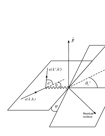
Figure 13: Leptonic and hadronic planes for hypernuclei electroproduction.

The right-handed coordinate system is completed by defining

$$\hat{{\bf y}} = \hat{{\bf z}}\times\hat{{\bf x}}.$$ (71)

In the leptonic plane the electron scattering angle is $\theta^{\prime}$, and the direction of the incident electron with respect to the $\hat{{\bf z}}$ is denoted by the angle $\alpha$. In the hadronic plane the meson scattering angle is denoted by $\theta_{1}^{\prime}$. The hadronic plane makes an angle $\phi$ with respect to the leptonic plane. The three-momentum of the incoming electron ${\bf k}$ (defined with respect to the coordinate system in Fig. 13) is given by, for massless electrons,

$${\bf k} = \left(E_{k}\sin\alpha\right)\,{\bf\hat{x}}+\left(E_{k}\cos\alpha\right)\,{\bf\hat{z}}.$$ (72)

The energy transfer to the nucleus is given by

$$q_{0} = E_{k}-E_{k^{\prime}}.$$ (73)

The three-momentum of the outgoing electron ${\bf k^{\prime}}$ is given by

$${\bf k^{\prime}} = \left[E_{k^{\prime}}\sin(\alpha+\theta^{\prime})\right]{\bf\hat{x}}+\left[E_{k^{\prime}}\cos(\alpha+\theta^{\prime})\right]{\bf\hat{z}}.$$ (74)

Since the virtual photon direction defines the ${\bf\hat{z}}$-axis, it follows that ${\bf q}\,=\,(0,0,|{\bf q}|)$, and therefore we can determine the angle $\alpha$ in Fig. 13 by demanding that $q_{x}\,=\,k_{x}-k_{x}^{\prime}$ should be zero. This yields the following equation for the angle $\alpha$:

$$\sin^{2}\alpha = \displaystyle\frac{E_{k^{\prime}}^{2}\,\sin^{2}\theta^{\prime}}{E_{k}^{2}+E_{k^{\prime}}^{2}-2E_{k}E_{k^{\prime}}\,\cos\theta^{\prime}}.$$ (75)

Geometric arguments show that the laboratory three-momentum of the outgoing meson is given by

$${\bf p_{1}^{\prime}} = \sqrt{E_{p_{1}^{\prime}}-M_{K}^{2}}\,\left[\,\left(\sin\theta_{1}^{\prime}\cos\phi^{\prime}\right)\,{\bf\hat{x}}+\left(\sin\theta_{1}^{\prime}\sin\phi^{\prime}\right)\,{\bf\hat{y}}+\left(\cos\theta_{1}^{\prime}\right)\,{\bf\hat{z}}\,\right].$$ (76)

To proceed any further in specifying the kinematics, we need to determine the energy of the outgoing meson $E_{p_{1}^{\prime}}$. This is done by using the Dirac delta function in Eq. (69). The total energy of the residual hypernucleus is given by

$$E_{P^{\prime}} = \sqrt{{\bf P^{\prime}}+_{\Lambda}M_{A}}\,=\,\sqrt{\left({\bf q}-{\bf p_{1}^{\prime}}\,\right)^{2}+_{\Lambda}M_{A}}$$ (77)

$$= \sqrt{\left({\bf q}-{\bf p_{1}^{\prime}}\,\right)^{2}+\left[M_{A}-\left(M_{p}-E_{B}^{(N)}\right)+\left(M_{Y}-E_{B}^{(Y)}\right)\,\right]^{2}}$$ (78)

where $E_{B}^{(N)}$ and $E_{B}^{(Y)}$ are the bound state energies for the nucleon and hyperon orbitals, respectively. These two quantities will be obtained from a relativistic mean-field model of the nuclear structure (see Sec. II.3.1). The quantity $E_{P^{\prime}}$ can be written as a function of the outgoing meson energy $E_{p_{1}^{\prime}}$. In addition, using the relations

$$d^{3}{\bf k^{\prime}} = 2\pi E_{k^{\prime}}^{2}\,dE_{k^{\prime}}\,d\left(\cos\theta^{\prime}\,\right),$$ (79)

$$d^{3}{\bf p_{1}^{\prime}} = \sqrt{E_{p_{1}^{\prime}}^{2}-M_{K}^{2}}\,E_{p_{1}^{\prime}}\,dE_{p_{1}^{\prime}}\,d\Omega_{1}^{\prime}$$ (80)

the triple differential cross section for the electromagnetic production of hypernuclei can be written as

$$\displaystyle\frac{d\sigma}{dE_{k^{\prime}}\,d\left(\cos\theta^{\prime}\,\right)\,d\Omega_{1}^{\prime}} = \displaystyle\frac{E_{k^{\prime}}^{2}\,\sqrt{E_{p_{1}^{\prime}}^{2}-M_{K}^{2}}}{2\left(2\pi\right)^{4}|f^{\prime}(E_{p_{1}^{\prime}})\,|}\,|{\cal M}|^{2}$$ (81)

where the energy of the outgoing meson $E_{p_{1}^{\prime}}$ is obtained by finding the roots of the equation

$$f(E_{p_{1}^{\prime}}) = E_{k}+M_{A}-E_{k^{\prime}}-E_{p_{1}^{\prime}}-\left[{\bf q}^{2}+E_{p_{1}^{\prime}}^{2}-M_{K}^{2}-2|{\bf q}|\,\sqrt{E_{p_{1}^{\prime}}^{2}-M_{K}^{2}}\,\cos\theta_{1}^{\prime}+\right.$$ (82)

$$\left.\left(M_{A}-M_{p}+M_{Y}+E_{B}^{(N)}-E_{B}^{(Y)}\,\right)^{2}\,\right]^{\frac{1}{2}}$$

where

$$|{\bf q}| = \left[E_{k}^{2}+E_{k^{\prime}}^{2}-2E_{k}\,E_{k^{\prime}}\,\cos\theta^{\prime}\,\right]^{\frac{1}{2}}.$$ (83)

We can see that the leptonic four-vectors, as well as the outgoing meson four-vector are fully determined if we specify the following kinematical quantities $\left[E_{k},E_{k^{\prime}},\theta^{\prime},\Omega_{1}^{\prime}\equiv\left(\theta_{1}^{\prime},\phi^{\prime}\,\right)\,\right]$.

Appendix B Leptonic and hadronic tensors

The transition matrix element ${\cal M}$ for the electromagnetic production of hypernuclei may be defined as

$${\cal M} = \left[\overline{U}({\bf k^{\prime}},h^{\prime}\,)\gamma_{\mu}\,U({\bf k},h)\,\right]\,\left(\frac{e^{2}}{q^{2}}\right)\,\langle\,p_{1}^{\prime};\,_{\Lambda}\Psi(P^{\prime}\,)\,|\hat{J}^{\mu}(q)\,|\Psi(P)\,\rangle$$ (84)

with $e^{2}/4\pi\,=\,1/137$. In Eq. (84) $\hat{J}^{\mu}$ is the nuclear current operator. Since we are neglecting the electron mass with respect to the total energy, we employ the helicity representation van der Ventel and Piekarewicz (2004) of the plane wave Dirac spinor

$$U({\bf k},h) = \displaystyle\frac{1}{\sqrt{2}}\,\left(\begin{array}[]{c}\phi_{h}({\bf\hat{k}})\\[14.22636pt] h\phi_{h}({\bf\hat{k}})\end{array}\right)$$ (87)

with

$$\phi_{h^{\prime}}({\bf\hat{k}^{\prime}}) = \left(\begin{array}[]{c}\delta_{h^{\prime},1}\,\cos\displaystyle\frac{\theta^{\prime}}{2}-\delta_{h^{\prime},-1}\,e^{-i\phi^{\prime}}\,\sin\displaystyle\frac{\theta^{\prime}}{2}\\[7.11317pt] \delta_{h^{\prime},1}\,e^{i\phi^{\prime}}\,\sin\displaystyle\frac{\theta^{\prime}}{2}+\delta_{h^{\prime},-1}\,\cos\displaystyle\frac{\theta^{\prime}}{2}\end{array}\right)$$ (90)

where the unit vector ${\bf\hat{k}}$ is specified by the polar and azimuthal angles, $\theta$ and $\phi$, respectively. This spinor is non-covariantly normalized to $U^{\dagger}U\,=\,1$, and corresponds to the normalization adopted for the bound state spinors. See Sec. II.3. It follows that $|{\cal M}|^{2}$ can be written as a contraction between the leptonic and hadronic tensors, i.e.,

$$|{\cal M}|^{2} = \left(\frac{e^{2}}{q^{2}}\right)^{2}\,\ell_{\mu\nu}\,{\cal W}^{\mu\nu}$$ (91)

where

$$\ell_{\mu\nu} = \left[\,\overline{U}({\bf k^{\prime}},h^{\prime}\,)\gamma_{\mu}\,U({\bf k},h)\,\right]\,\left[\,\overline{U}({\bf k^{\prime}},h^{\prime}\,)\gamma_{\nu}\,U({\bf k},h)\,\right]^{*}$$ (92)

and

$${\cal W}^{\mu\nu} = \langle\,p_{1}^{\prime};\,_{\Lambda}\Psi(P^{\prime}\,)\,|\hat{J}^{\mu}(q)\,|\Psi(P)\,\rangle\,\langle\,p_{1}^{\prime};\,_{\Lambda}\Psi(P^{\prime}\,)\,|\hat{J}^{\nu}(q)\,|\Psi(P)\,\rangle^{*}.$$ (93)

We will now study each one of these tensors in detail. The leptonic tensor may be written as a trace over Dirac matrices. This is done by using the identity

$$U({\bf k},h)\,\overline{U}({\bf k^{\prime}},h^{\prime}\,) = \displaystyle\frac{\hbox to0.0pt{/\hss}k}{4E_{k}}\,\left(1-h\gamma^{5}\,\right).$$ (94)

It follows from Eq. (94) that the leptonic tensors will in general be dependent on the helicity of the incoming and outgoing electrons. We may therefore distinguish four different cases for the leptonic tensor. In the first case both the incident and outgoing electron beams are unpolarized. In this case we define

$$\ell^{(0)}_{\mu\nu} = \mbox{Tr}\,\left[\gamma_{\mu}\;\left(\sum_{h\,=\,\pm 1}\,U({\bf k},h)\,\overline{U}({\bf k},h)\,\right)\,\gamma_{\nu}\,\left(\sum_{h^{\prime}\,=\,\pm 1}\,U({\bf k^{\prime}},h^{\prime})\,\overline{U}({\bf k^{\prime}},h^{\prime}\,)\,\right)\,\right]$$ (95)

$$= \displaystyle\frac{1}{E_{k}\,E_{k^{\prime}}}\,\left(k_{\mu}\,k_{\nu}^{\prime}+k_{\mu}^{\prime}k_{\nu}-k\cdot k^{\prime}\,g_{\mu\nu}\right).$$ (96)

Note that $\ell^{(0)}_{\mu\nu}$ is completely symmetric in $\mu$ and $\nu$. In the second case the incident electron beam is polarized and the outgoing electron beam is unpolarized. In this case we define

$$\ell^{(1)}_{\mu\nu}(k,h;k^{\prime}\,) = \mbox{Tr}\left[\gamma_{\mu}\,\left(U({\bf k},h)\,\overline{U}({\bf k},h)\,\right)\,\gamma_{\nu}\,\left(\sum_{h^{\prime}\,=\,\pm 1}\,U({\bf k^{\prime}},h^{\prime})\,\overline{U}({\bf k^{\prime}},h^{\prime}\,)\right)\,\right]$$ (97)

$$= \displaystyle\frac{1}{2}\,\ell^{(0)}_{\mu\nu}-\displaystyle\frac{ih}{2E_{k}E_{k^{\prime}}}\,k^{\alpha}\,k^{\prime\beta}\,\epsilon_{\mu\nu\alpha\beta}$$ (98)

where we adopt the convention $\epsilon^{0123}\,=\,+1$ for the Levi-Civita tensor. Note that the lepton tensor now contains an anti-symmetric term due to the polarization of the incoming electron beam. If the incident beam is unpolarized and the outgoing beam is polarized then we define

$$\ell^{(2)}_{\mu\nu}(k;k^{\prime},h^{\prime}\,) = \mbox{Tr}\left[\gamma_{\mu}\,\left(\sum_{h^{\prime}\,=\,\pm}\,U({\bf k},h)\,\overline{U}({\bf k},h)\right)\,\gamma_{\nu}\,\left(U({\bf k^{\prime}},h^{\prime})\,\overline{U}({\bf k^{\prime}},h^{\prime})\right)\,\right]$$ (99)

$$= \ell^{(1)}_{\nu\mu}(k^{\prime},h^{\prime};k).$$ (100)

In the final case the incoming and outgoing beams are polarized. Now

$$\ell_{\mu\nu}(k,h;k^{\prime},h^{\prime}\,) = \mbox{Tr}\,\left[\gamma_{\mu}\,\left(U({\bf k},h)\,\overline{U}({\bf k},h)\,\right)\,\gamma_{\nu}\,\left(U({\bf k^{\prime}},h^{\prime})\,\overline{U}({\bf k^{\prime}},h^{\prime}\,)\,\right)\,\right]$$ (101)

$$= \displaystyle\frac{1+hh^{\prime}}{4}\,\ell^{(0)}_{\mu\nu}+\displaystyle\frac{i(h+h^{\prime}\,)}{4E_{k}E_{k^{\prime}}}\,k^{\alpha}\,k^{\prime\beta}\,\epsilon_{\mu\nu\alpha\beta}.$$ (102)

Next we turn our attention to the hadronic tensor ${\cal W}^{\mu\nu}$. The definition in Eq. (93) shows that this is an extremely complicated object since it contains exact many-body wave functions. However, ${\cal W}^{\mu\nu}$ can only be a function of the three independent four-momenta, namely $q^{\mu}$, $P^{\mu}$ and $p_{1}^{\prime\mu}$. Note that four-momentum conservation fixes

$$P^{\prime} = q+P-p_{1}^{\prime}.$$ (103)

We can therefore expand ${\cal W}^{\mu\nu}$ in terms of a basis constructed from $\{g^{\mu\nu},q^{\mu},P^{\mu},p_{1}^{\prime\mu}\}$. This is similar to the approach in Ref. van der Ventel and Piekarewicz (2004) with the exception that a parity conserving electromagnetic current forbids the presence of any terms linear in the Levi-Civita tensor. The expansion for ${\cal W}^{\mu\nu}$ then assumes the form

$${\cal W}^{\mu\nu} = W_{1}^{\prime}\,g^{\mu\nu}+W_{2}^{\prime}\,q^{\mu}q^{\nu}+W_{3}^{\prime}\,P^{\mu}P^{\nu}+W_{4}^{\prime}\,p_{1}^{\prime\mu}p_{1}^{\prime\nu}+W_{5}^{\prime}\,\left(P^{\mu}q^{\nu}+q^{\mu}P^{\nu}\,\right)+$$ (104)

$$W_{6}^{\prime}\,\left(p_{1}^{\prime\mu}q^{\nu}+q^{\mu}p_{1}^{\prime\nu}\,\right)+W_{7}^{\prime}\,\left(p_{1}^{\prime\mu}P^{\nu}+P^{\mu}p_{1}^{\prime\nu}\,\right)+W_{8}^{\prime}\,\left(P^{\mu}q^{\nu}-q^{\mu}P^{\nu}\,\right)+$$

$$W_{9}^{\prime}\,\left(p_{1}^{\prime\mu}q^{\nu}-q^{\mu}p_{1}^{\prime\nu}\,\right)+W_{10}^{\prime}\,\left(p_{1}^{\prime\mu}P^{\nu}-P^{\mu}p_{1}^{\prime\nu}\,\right).$$

At this point ${\cal W}^{\mu\nu}$ contains ten independent nuclear structure functions. However, the imposition of electromagnetic current conservation, i.e.,

$$q_{\mu}{\cal W}^{\mu\nu}\,=\,q_{\nu}{\cal W}^{\mu\nu} = 0$$ (105)

reduces the hadronic tensor to the following form Picklesimer et al. (1985)

$${\cal W}^{\mu\nu} = W_{1}\,G^{\mu\nu}+W_{2}\,A^{\mu}A^{\nu}+W_{3}\,B^{\mu}B^{\nu}+W_{4}\,\left(A^{\mu}B^{\nu}+B^{\mu}A^{\nu}\,\right)+$$ (106)

$$W_{5}\,\left(A^{\mu}B^{\nu}-B^{\mu}A^{\nu}\,\right)$$

where

$$G^{\mu\nu} = g^{\mu\nu}-\displaystyle\frac{q^{\mu}q^{\nu}}{q^{2}}$$ (107)

$$A^{\mu} = P^{\mu}-\displaystyle\frac{P\cdot q}{q^{2}}\,q^{\mu}$$ (108)

$$B^{\mu} = p_{1}^{\prime\mu}-\displaystyle\frac{p_{1}^{\prime}\cdot q}{q^{2}}\,q^{\mu}.$$ (109)

Note that

$$A\cdot q\,=\,B\cdot q = 0.$$ (110)

The hadronic tensor consists of four terms which are symmetric with respect to $\mu$ and $\nu$, and the last term which is anti-symmetric with respect to $\mu$ and $\nu$, hence

$${\cal W}^{\mu\nu} = {\cal W}_{S}^{\mu\nu}+{\cal W}_{A}^{\mu\nu}\,=\,\sum_{i\,=\,1}^{4}\,W_{i}\,u_{i}^{\mu\nu}+W_{5}\,u_{5}^{\mu\nu}$$ (111)

where

$$\{u_{1}^{\mu\nu},u_{2}^{\mu\nu},u_{3}^{\mu\nu},u_{4}^{\mu\nu},u_{5}^{\mu\nu}\} = \{G^{\mu\nu},A^{\mu}A^{\nu},B^{\mu}B^{\nu},A^{\mu}B^{\nu}+B^{\mu}A^{\nu},A^{\mu}B^{\nu}-B^{\mu}A^{\nu}\}.$$ (112)

Since the contraction of a symmetric and an anti-symmetric tensor is zero, it follows immediately that

$$W_{5} = \displaystyle\frac{u_{5,\mu\nu}\,{\cal W}^{\mu\nu}}{u_{5,\mu\nu}\,u_{5}^{\mu\nu}}.$$ (113)

Since the basis $\{u_{i}^{\mu\nu}\}$ is not orthogonal, we can determine the structure functions $W_{i}\,(i\,=\,1,2,3,4)$ by solving the following set of coupled linear equations

$$\underline{W}_{U} = U\,\underline{W}$$ (114)

where

$$\left(\underline{W}_{U}\,\right)_{i} = u_{i,\mu\nu}\,{\cal W}^{\mu\nu},\qquad i\,=\,1,2,3,4$$ (115)

and the $4\times 4$ matrix $U$ is given by

$$U = \left(\begin{array}[]{cccc}3&\hskip 14.22636ptA^{2}&\hskip 14.22636ptB^{2}&\hskip 14.22636pt2A\cdot B\\[7.11317pt] A^{2}&\hskip 14.22636ptA^{4}&\hskip 14.22636pt\left(A\cdot B\right)^{2}&\hskip 14.22636pt2A^{2}\,\left(A\cdot B\right)\\[7.11317pt] B^{2}&\hskip 14.22636pt\left(A\cdot B\right)^{2}&\hskip 14.22636ptB^{4}&\hskip 14.22636pt2B^{2}\left(A\cdot B\right)\\[7.11317pt] 2A\cdot B&\hskip 14.22636pt2A^{2}\,\left(A\cdot B\right)&\hskip 14.22636pt2B^{2}\,\left(A\cdot B\right)&\hskip 14.22636pt2A^{2}B^{2}+2\left(A\cdot B\right)^{2}\end{array}\right)$$ (120)

with

$$\underline{W} = \left(\begin{array}[]{c}W_{1}\\[7.11317pt] W_{2}\\[7.11317pt] W_{3}\\[7.11317pt] W_{4}\end{array}\right).$$ (125)

Using the general expansion of ${\cal W}^{\mu\nu}$ we can now work out its contraction with $\ell_{\mu\nu}$. As shown previously, the leptonic tensor can be written in four different forms, depending on whether the incident and/or outgoing electron beams are polarized or not. The four contractions are

$$|{\cal M}^{(0)}\,|^{2} = \left(\frac{e^{2}}{q^{2}}\right)^{2}\,\ell_{\mu\nu}^{(0)}\,{\cal W}^{\mu\nu}_{S}$$ (126)

$$= \displaystyle\left(\frac{e^{2}}{q^{2}}\right)^{2}\,\frac{1}{E_{k}\,E_{k^{\prime}}}\,\left[W_{1}\,\left(-3k\cdot k^{\prime}+2f_{1}(k,k^{\prime}\,)\,\right)+W_{2}\,\left(-k\cdot k^{\prime}\,f_{1}(P,P)+\right.\right.$$

$$\left.2f_{1}(k,P)\,f_{1}(k^{\prime},P)\,\right)+W_{3}\,\left(-k\cdot k^{\prime}\,f_{1}(p_{1}^{\prime},p_{1}^{\prime}\,)+2f_{1}(k,p_{1}^{\prime})\,f_{1}(k^{\prime},p_{1}^{\prime}\,)\right)+$$

$$\left.W_{4}\,\left(2f_{2}(P,p_{1}^{\prime}\,)\,\right)\,\right],$$

$$|{\cal M}^{(1)}\,|^{2} = \left(\frac{e^{2}}{q^{2}}\right)^{2}\,\ell_{\mu\nu}^{(1)}(k,h;k^{\prime}\,)\,{\cal W}^{\mu\nu}$$ (127)

$$= \displaystyle\left(\frac{e^{2}}{q^{2}}\right)^{2}\,\left[\frac{1}{2}\,\ell_{\mu\nu}^{(0)}\,{\cal W}^{\mu\nu}_{S}-\displaystyle\frac{ih}{2E_{k}\,E_{k^{\prime}}}\,k^{\alpha}\,k^{\prime\beta}\,\epsilon_{\mu\nu\alpha\beta}\,\left(A^{\mu}B^{\nu}-B^{\mu}A^{\nu}\,\right)\,W_{5}\,\right],$$ (128)

$$|{\cal M}^{(2)}\,|^{2} = \left(\frac{e^{2}}{q^{2}}\right)^{2}\,\ell_{\mu\nu}^{(2)}(k;k^{\prime},h^{\prime}\,)\,{\cal W}^{\mu\nu}\,=\,\left(\frac{e^{2}}{q^{2}}\right)^{2}\,\ell_{\nu\mu}^{(1)}(k^{\prime},h^{\prime};k)\,{\cal W}^{\mu\nu},$$ (129)

$$|{\cal M}\,|^{2} = \left(\frac{e^{2}}{q^{2}}\right)^{2}\,\ell_{\mu\nu}(k,h;k^{\prime},h^{\prime}\,)\,{\cal W}^{\mu\nu}$$ (130)

$$= \left(\frac{e^{2}}{q^{2}}\right)^{2}\,\left[\displaystyle\frac{1+hh^{\prime}}{4}\,\ell_{\mu\nu}^{(0)}\,{\cal W}^{\mu\nu}_{S}-\displaystyle\frac{i(h+h^{\prime}\,)}{4E_{k}\,E_{k^{\prime}}}\,k^{\alpha}\,k^{\beta}\,\epsilon_{\mu\nu\alpha\beta}{\cal W}^{\mu\nu}_{A}\right]$$ (131)

where

$$f_{1}(x,y) = x\cdot y-\displaystyle\frac{x\cdot q\,y\cdot q}{q^{2}}\,=\,f_{1}(y,x)$$ (132)

$$f_{2}(x,y) = f_{1}(k,x)\,f_{1}(k^{\prime},y)+f_{1}(k^{\prime},x)\,f_{1}(k,y)-k\cdot k^{\prime}\,f_{1}(x,y).$$ (133)

We can now substitute Eqs. (126), (128), (129) or (131) into Eq. (81) to obtain an unpolarized, partially polarized or fully polarized cross section. The resulting cross section will only depend on kinematical quantities (determined by the experimental set-up), and a set of nuclear structure functions.

References

• Gibson (1995) B. F. Gibson, Phys. Rept. 257, 349 (1995).
• Hinton (2000) W. Hinton, Ph.D. thesis, Hampton University (2000).
• Hungerford (2001) E. V. Hungerford, Nucl. Phys. A691, 21 (2001).
• Cohen (1985) J. Cohen, Phys. Rev. C32, 543 (1985).
• Mart and Bennhold (1999) T. Mart and C. Bennhold, Phys. Rev. C61, 012201 (1999), eprint nucl-th/9906096.
• Niculescu et al. (1998) G. Niculescu et al., Phys. Rev. Lett. 81, 1805 (1998).
• Tamura (2004) H. Tamura, Prog. Theor. Phys. Suppl. 156, 104 (2004).
• Schumacher (1995) R. A. Schumacher, Nucl. Phys. A585, 63c (1995).
• Mohring et al. (2003) R. M. Mohring et al. (E93018), Phys. Rev. C67, 055205 (2003), eprint nucl-ex/0211005.
• Zhu (2001) X. Zhu, Ph.D. thesis, Graduate college of China Institute of Atomic Energy (2001).
• Yuan (2002) L. Yuan, Ph.D. thesis, Hampton University (2002).
• Miyoshi et al. (2003) T. Miyoshi et al. (HNSS), Phys. Rev. Lett. 90, 232502 (2003), eprint nucl-ex/0211006.
• Koltenuk (1999) D. M. Koltenuk, Ph.D. thesis, University of Pennsylvania (1999).
• Cha (2000) J. Cha, Ph.D. thesis, Hampton University (2000).
• Uzzle (2002) A. Uzzle, Ph.D. thesis, Hampton University (2002).
• Dohrmann et al. (2004) F. Dohrmann et al. (Jefferson Lab E91-016), Phys. Rev. Lett. 93, 242501 (2004), eprint nucl-ex/0412027.
• McNabb et al. (2004) J. W. C. McNabb et al., Phys. Rev. C69, 042201 (2004).
• Thom (1966) H. Thom, Phys. Rev. C151, 1322 (1966).
• Deo and Bisoi (1974) B. B. Deo and A. K. Bisoi, Phys. Rev. C9, 288 (1974).
• Cotanch and Hsiao (1986) S. R. Cotanch and S. S. Hsiao, Nucl. Phys. A450, 419c (1986).
• Ji and Cotanch (1988) C.-R. Ji and S. R. Cotanch, Phys. Rev. C38, 2691 (1988).
• Tanabe et al. (1989) H. Tanabe, M. Kohno, and C. Bennhold, Phys. Rev. C39, 741 (1989).
• Adelseck and Saghai (1990) R. A. Adelseck and B. Saghai, Phys. Rev. C42, 108 (1990).
• Williams et al. (1991) R. A. Williams, C. R. Ji, and S. R. Cotanch, Phys. Rev. C43, 452 (1991).
• Williams et al. (1992) R. A. Williams, C. R. Ji, and S. R. Cotanch, Phys. Rev. C46, 1617 (1992).
• David et al. (1996) J. C. David, C. Fayard, G. H. Lamot, and B. Saghai, Phys. Rev. C53, 2613 (1996).
• Mizutani et al. (1998) T. Mizutani, C. Fayard, G. H. Lamot, and B. Saghai, Phys. Rev. C58, 75 (1998), eprint nucl-th/9712037.
• Bennhold et al. (1999) C. Bennhold, H. Haberzettl, and T. Mart (1999), eprint nucl-th/9909022.
• Bydzovsky and Sotona (2005) P. Bydzovsky and M. Sotona, Nucl. Phys. A754, 243 (2005), eprint nucl-th/0408039.
• Mart and Bennhold (2004) T. Mart and C. Bennhold (2004), eprint nucl-th/0412097.
• Saghai (2003) B. Saghai (2003), eprint nucl-th/0310025.
• Hsiao and Cotanch (1983) S. S. Hsiao and S. R. Cotanch, Phys. Rev. C28, 1668 (1983).
• Rosenthal et al. (1988) A. S. Rosenthal, D. Halderson, K. Hodgkinson, and F. Tabakin, Ann. Phys. 184, 33 (1988).
• Bennhold and Wright (1989) C. Bennhold and L. E. Wright, Phys. Rev. C39, 927 (1989).
• Bennhold and Wright (1988) C. Bennhold and L. E. Wright, Prog. Part. Phys. Nucl. 20, 377 (1988).
• Lee et al. (2001) F. X. Lee, T. Mart, C. Bennhold, and L. E. Wright, Nucl. Phys. A695, 237 (2001), eprint nucl-th/9907119.
• Motoba et al. (1994) T. Motoba, M. Sotona, and K. Itonaga, Prog. Theor. Phys. Suppl. 117, 123 (1994).
• Bennhold (1989) C. Bennhold, Phys. Rev. C39, 1944 (1989).
• Bennhold (1991) C. Bennhold, Phys. Rev. C43, 775 (1991).
• Sotona and Frullani (1994) M. Sotona and S. Frullani, Prog. Theor. Phys. Suppl. 117, 151 (1994).
• Picklesimer and Tandy (1986) A. Picklesimer and P. C. Tandy, Phys. Rev. C34, 1860 (1986).
• van der Ventel and Piekarewicz (2004) B. I. S. van der Ventel and J. Piekarewicz, Phys. Rev. C 69, 035501 (2004), eprint nucl-th/0310047.
• van der Ventel and Piekarewicz (2006) B. I. S. van der Ventel and J. Piekarewicz, Phys. Rev. C73, 025501 (2006), eprint nucl-th/0506071.
• Serot and Walecka (1986) B. D. Serot and J. D. Walecka, Adv. Nucl. Phys. 16, 1 (1986).
• Lalazissis et al. (1997) G. A. Lalazissis, J. Konig, and P. Ring, Phys. Rev. C 55, 540 (1997).
• Todd-Rutel and Piekarewicz (2005) B. G. Todd-Rutel and J. Piekarewicz (2005), eprint [http://xxx.lanl.gov/abs]nucl-th/0504034.
• Picklesimer et al. (1985) A. Picklesimer, J. W. Van Orden, and S. J. Wallace, Phys. Rev. C32, 1312 (1985).
• Lu et al. (2003) H. F. Lu, J. Meng, S. Q. Zhang, and S.-G. Zhou, J. Eur. Phys. A17, 19 (2003).