Convergence of Perturbations for a Big Bounce in Loop Quantum Cosmology

Abstract

We investigate the convergence behaviors of the scalar and the vector perturbations for a big bounce phase in loop quantum cosmology. Two models are discussed: one is the universe filled by a massless scalar field; the other is a toy model which is radiation-dominated in the asymptotic past and future. We find that the behaviors of the Bardeen potential of the scalar mode near both the bounce point and the transition point of the null energy condition are good, moreover, the unlimited growth of the vector perturbation can be avoided in our bounce model. This is different from the bounce models in pure general relativity. And we also find that the maximum of an observable vector mode is inversely proportional to the square of the minimum scalar factor $a_{bounce}$. This conclusion is independent with the bounce model, and we may conclude that the bounce in loop quantum cosmology is reasonable.

I Introduction

There are several ways to solve the singularity problem in cosmology r7 , one of them is the bounce model r8 ; r9 ; r10 . In the studying of the bounce model in pure general relativity (GR) r11 , the scalar hydrodynamic perturbation can lead to a singular behavior of the Bardeen potential. The further study r12 ; r13 ; r14 show that the divergence of the Bardeen potential can be avoided only in some models with special matter.

Another mode of perturbations must be considered is the vector perturbation. It is known that the vector mode will decay quickly in expanding phase of the universe. So it exhibits a growing mode solution in a contracting universe r97 . This growing will in general lead to the breakdown of perturbation theory near the bounce. So, it is necessary to check the behaviors of the vector perturbations near the bounce.

Generally speaking, the bouncing phase originates from a quantum effect of gravity. So it is interesting to study the bounce model in quantum gravity theory.

At present, the issue of finding a complete theory of quantum gravity is still open. In current approaches, one of the most active is loop quantum gravity. Loop quantum gravity (LQG) lqg1 ; lqg2 ; lqg3 is a mathematically well-defined, non-perturbative and background independent quantization of general relativity. And, Loop Quantum Cosmology (LQC) B , a symmetry reduction of LQG to the homogeneous and isotropic spacetime, has achieved many successes. A major success of LQC is the resolution of the Big Bang singularity bb ; nbb1 ; nbb2 , this result depends crucially on the discreteness of the spacetime. Instead of Big Bang, there will be a Big Bounce.

In GR bounce, the divergence of the Bardeen potential occurs at two point r11 , i.e., near the bounce point and near the transition point of null energy condition (NEC). The difference is that the LQC bounce is governed by a discrete quantum geometry r15 . This will lead to some different behaviors of the Bardeen potential. In this paper, we consider the behaviors of the perturbations near both the bounce point and the transition point of NEC under the framework of the effective theory of LQC.

The paper is organized as follows. In Sec. II, we give the framework of the effective theory of LQC with holonomy corrections, it can yield the bounce background. In Sec.III, we introduce the scalar perturbation based on the Sec. II. Two models are analyzed in this section: one is the universe filled by a massless scalar field; the other is a toy model which is radiation-dominated in the asymptotic past and future. In Sec. IV we discuss the vector perturbation near the bounce. The discussion and conclusions are presented in Sec. V.

II background of LQC bounce

The canonical variables used in LQG are the Ashtekar connection $A_{a}^{i}$ and the densitized triad $E_{i}^{a}$ lqg1 ; lqg2 ; lqg3 , where $A_{a}^{i}=\Gamma_{a}^{i}+K_{a}^{i}$ with $\Gamma$ the spin connection and $K$ the extrinsic curvature, and $E_{i}^{a}=e_{i}^{a}/|dete_{i}^{b}|$ with $e_{i}^{a}e_{i}^{b}=q^{ab}$ and $q_{ab}$ the spatial metric. For a spatially homogeneous and isotropic universe model (FRW metric), the Ashtekar variables can be reduced to the diagonal form, i.e., $A^{i}_{a}=c\delta^{i}_{a}$ and $E^{a}_{i}=p\delta^{a}_{i}$ B . Therefore, the basic canonical variables for the gravitational field are $(\bar{c},\bar{p})$ and for the scalar field $(\bar{\varphi},p_{\bar{\varphi}})$. Here we denote the background variables with a bar. In this paper, we consider only the flat space universe. Thus the canonical variables can be expressed in terms of the standard FRW variables as: $(\bar{c},|\bar{p}|)=(\gamma\dot{a},a^{2})$, where $a$ is the scale factor; and the effective Hamlitonian of the considered model is given by

$$H=-\frac{3}{8\pi G\gamma^{2}}\sqrt{|\bar{p}|}\bar{c}^{2}+\frac{1}{2}\frac{p_{\bar{\varphi}}^{2}}{|\bar{p}|^{3/2}}+|\bar{p}|^{3/2}V(\bar{\varphi}),$$ (1)

where the factor $\gamma$ is called the Barbero-Immirzi parameter which is a constant of the theory.

In the process of quantization, we can find that there is no operator corresponding to the canonical variable $\bar{c}$ itself but we can return to the holonomy. This fact can lead to the so-called holonomy correction in an effective theory of LQC. The effects of this correction can be obtain by simply replacing the $\bar{c}$ to $\sin(\tilde{\mu}\bar{c})/\tilde{\mu}$ with the choice of

$$\tilde{\mu}=\sqrt{\frac{\Delta}{|\bar{p}|}},$$ (2)

where $\Delta\equiv 2\sqrt{3}\pi\gamma l_{p}^{2}$ is a area gap, and $l_{p}$ denotes the Planck length. So, the effective Hamiltonian with holonomy correction is

$$H_{eff}=-\frac{3}{8\pi G\gamma^{2}}\sqrt{|\bar{p}|}\left[\frac{\sin(\tilde{\mu}\bar{c})}{\tilde{\mu}}\right]^{2}+\frac{1}{2}\frac{p_{\bar{\varphi}}^{2}}{|\bar{p}|^{3/2}}+|\bar{p}|^{3/2}V(\bar{\varphi}).$$ (3)

From now on, we focus on a positive $\bar{p}$.

The equations of motion can now be derived by the using of the Hamilton equation

$$\dot{f}=\{f,H_{eff}\},$$ (4)

where the dot denotes the derivative with respect to the cosmic time $t$ and the Poisson bracket is defined as

$$\{f,g\}= \frac{8\pi G\gamma}{3}\left[\frac{\partial f}{\partial\bar{c}}\frac{\partial g}{\partial\bar{p}}-\frac{\partial f}{\partial\bar{p}}\frac{\partial g}{\partial\bar{c}}\right]$$ (5)

$$+ \left[\frac{\partial f}{\partial\bar{\varphi}}\frac{\partial g}{\partial p_{\bar{\varphi}}}-\frac{\partial f}{\partial p_{\bar{\varphi}}}\frac{\partial g}{\partial\bar{\varphi}}\right].$$

From this definition we can obtain two elementary brackets

$$\{\bar{c},\bar{p}\}=\frac{8\pi G\gamma}{3},\ \ \ \ \{\bar{\varphi},p_{\bar{\varphi}}\}=1.$$ (6)

By using these brackets, one can derive two equations, i.e., an effective Friedmann equation and an effective Raychaudhuri equation. However, in theory of perturbation, the use of the conformal time $\eta$ may be convenient than the cosmic time. The conformal time can be related to the cosmic time $t$ through the scale factor $a$, $ad\eta=dt$. Thence the effective Friedmann equation and the effective Raychaudhuri equation with conformal time are respectively r1 ,

$$\left[\frac{\sin(\tilde{\mu}\gamma\bar{\mathfrak{K}})}{\gamma\tilde{\mu}}\right]^{2}=\frac{8\pi G}{3}\left[\frac{1}{2}(\bar{\varphi}^{\prime})^{2}+\bar{p}V(\bar{\varphi})\right],$$ (7)

$$\bar{\mathfrak{K}}^{\prime} + \frac{1}{2}\left[\frac{\sin(\tilde{\mu}\gamma\bar{\mathfrak{K}})}{\gamma\tilde{\mu}}\right]^{2}+\bar{p}\frac{\partial}{\partial\bar{p}}\left[\frac{\sin(\tilde{\mu}\gamma\bar{\mathfrak{K}})}{\gamma\tilde{\mu}}\right]^{2}$$ (8)

$$=4\pi G\left[-\frac{1}{2}(\bar{\varphi}^{\prime})^{2}+\bar{p}V(\bar{\varphi})\right],$$

where the prime denotes the derivative with respect to the conformal time $\eta$ and $\gamma\bar{\mathfrak{K}}\equiv\bar{c}$. In addition, the Klein-Gordon equation can also be derived as follows:

$$\bar{\varphi}^{\prime\prime}+2\left[\frac{\sin(2\tilde{\mu}\gamma\bar{\mathfrak{K}})}{2\gamma\tilde{\mu}}\right]\bar{\varphi}^{\prime}+\bar{p}V_{,\bar{\varphi}}(\bar{\varphi})=0.$$ (9)

From Eq.(4) and the relation between cosmic time and conformal time, one can get the motion equation of $\bar{p}$ with conformal time

$$\bar{p}^{\prime}=2\bar{p}\left[\frac{\sin(2\tilde{\mu}\gamma\bar{\mathfrak{K}})}{2\gamma\tilde{\mu}}\right].$$ (10)

So, one can further define a conformal Hubble parameter $\mathbb{H}$ by

$$\mathbb{H}:=\frac{\bar{p}^{\prime}}{2\bar{p}}=\frac{\sin(2\tilde{\mu}\gamma\bar{\mathfrak{K}})}{2\gamma\tilde{\mu}}.$$ (11)

Moreover, we can also define

$$\mathfrak{S}_{1} := \mathbb{H}^{2}-\left[\frac{\sin(\tilde{\mu}\gamma\bar{\mathfrak{K}})}{\gamma\tilde{\mu}}\right]^{2},$$ (12)

$$\mathfrak{S}_{2} := \mathbb{H}^{\prime}-\bar{\mathfrak{K}}^{\prime}-\bar{p}\frac{\partial}{\partial\bar{p}}\left[\frac{\sin(\tilde{\mu}\gamma\bar{\mathfrak{K}})}{\gamma\tilde{\mu}}\right]^{2}.$$ (13)

In fact, $\mathfrak{S}_{1}$ and $\mathfrak{S}_{2}$ can be taken as two effective corrections to the evolution equations of the Bardeen potential. This is because that one can obtain the classical evolution equations by taking $\mathfrak{S}_{1}\rightarrow 0$ and $\mathfrak{S}_{2}\rightarrow 0$ at the same time.

We rewrite the Eqs.(7) and (8) in terms of $\mathfrak{S}_{1}$, $\mathfrak{S}_{2}$ and $\mathbb{H}$

$$\mathbb{H}^{2}-\mathfrak{S}_{1}=\frac{8\pi G}{3}\bar{p}\times\rho_{s},$$ (14)

$$-\frac{1}{3}(\mathbb{H}^{2}-\mathfrak{S}_{1})-\frac{2}{3}(\mathbb{H}^{\prime}-\mathfrak{S}_{2})=\frac{8\pi G}{3}\bar{p}\times P_{s},$$ (15)

where

$$\rho_{s}:=\frac{(\bar{\varphi}^{\prime})^{2}}{2\bar{p}}+V(\bar{\varphi}),$$ (16)

and

$$P_{s}:=\frac{(\bar{\varphi}^{\prime})^{2}}{2\bar{p}}-V(\bar{\varphi})$$ (17)

are the energy density and pressure of scalar field respectively.

By using Eqs.(11) and (16), one can rewrite the Eq.(14) to

$$\mathbb{H}^{2}=l_{p}^{2}\bar{p}\ \rho_{s}\left(1-\frac{\rho_{s}}{\rho_{c}}\right),$$ (18)

where

$$\rho_{c}=\frac{1}{l_{p}^{2}\gamma^{2}\Delta}.$$ (19)

Obviously, one can easily check that when $\rho_{s}=\rho_{c}$, $\mathbb{H}=0$, and this means that a bounce occurs. The bounce density $\rho_{c}$ is related to $\Delta$ which is the smallest eigenvalue of area operator, so this LQC bounce is originated from the quantum effects of spacetime.

From Eqs.(14) and (15) we can get a useful relation equation

$$\rho_{s}+P_{s}=\frac{1}{4\pi G\bar{p}}\beta,$$ (20)

where

$$\beta:=\mathbb{H}^{2}-\mathbb{H}^{\prime}-\mathfrak{S}_{1}+\mathfrak{S}_{2}.$$ (21)

Thus, the relationship r3 between the null energy condition and the stress-energy tensor can be written as:

$$NEC\Longleftrightarrow\rho_{s}+P_{s}\geqslant 0\Longleftrightarrow\beta\geqslant 0.$$ (22)

III scalar perturbation with holonomy corrections

In this section, we introduce the scalar perturbation based on the Sec. II and analyze in detail the following two models: one is the universe filled by a massless scalar field; the other is a toy model which is radiation-dominated in the asymptotic past and future. In our models, the spacetime is described by the metric

$$ds^{2}=a^{2}(\eta)\left[-(1+2\Phi)d\eta^{2}+(1-2\Psi)\delta_{ab}dx^{a}dx^{b}\right],$$ (23)

where $\Phi$ and $\Psi$ are the Bardeen potential. In the case of vanishing anisotropic stresses, $\Phi$ and $\Psi$ are equal r4 . Therefore, we set $\Phi=\Psi$ from now on. The evolution equations of the Bardeen potential with holonomy corrections have been given in r1 :

$$\nabla^{2}\Phi-3\mathbb{H}\Phi^{\prime}-\left[\bar{\mathfrak{K}}^{\prime}+6\mathbb{H}^{2}-4\left[\frac{\sin(\tilde{\mu}\gamma\bar{\mathfrak{K}})}{\gamma\tilde{\mu}}\right]^{2}+\bar{p}\frac{\partial}{\partial\bar{p}}\left[\frac{\sin(\tilde{\mu}\gamma\bar{\mathfrak{K}})}{\gamma\tilde{\mu}}\right]^{2}\right]\Phi = 4\pi G\bar{p}\ \delta\rho_{s},$$

(24)

$$\Phi^{\prime\prime}+\left\{3\mathbb{H}+\frac{1}{\mathbb{H}}\left[\mathbb{H}^{\prime}-\bar{\mathfrak{K}}^{\prime}-\bar{p}\frac{\partial}{\partial\bar{p}}\left[\frac{\sin(\tilde{\mu}\gamma\bar{\mathfrak{K}})}{\gamma\tilde{\mu}}\right]^{2}\right]\right\}\Phi^{\prime}+\left[2\mathbb{H}^{2}+4\mathbb{H}^{\prime}-3\bar{\mathfrak{K}}^{\prime}-3\bar{p}\frac{\partial}{\partial\bar{p}}\left[\frac{\sin(\tilde{\mu}\gamma\bar{\mathfrak{K}})}{\gamma\tilde{\mu}}\right]^{2}\right]\Phi = 4\pi G\bar{p}\ \delta P_{s}.$$

By Using the definitions of Eqs.(12) and (13), we can rewrite the Eqs.(24) and (LABEL:e21) as

$$\nabla^{2}\Phi-3\mathbb{H}\Phi^{\prime}-\left[2\mathbb{H}^{2}+\mathbb{H}^{\prime}-4\mathfrak{S}_{1}-\mathfrak{S}_{2}\right]\Phi = 4\pi G\bar{p}\ \delta\rho_{s},$$

$$\Phi^{\prime\prime}+\left(3\mathbb{H}+\frac{\mathfrak{S}_{2}}{\mathbb{H}}\right)\Phi^{\prime}+\left[2\mathbb{H}^{2}+\mathbb{H}^{\prime}+3\mathfrak{S}_{2}\right]\Phi = 4\pi G\bar{p}\ \delta P_{s}.$$

We want to get the evolution equation of the Bardeen potential but the matter is not contained in it. So we should obtain the relationship between $\delta\rho_{s}$ and $\delta P_{s}$. In general, the pressure perturbation can be separated into two parts of the adiabatic and the entropic perturbation as follows

$$\delta P_{s}=\left(\frac{\partial P_{s}}{\partial\rho_{s}}\right)_{S}\delta\rho_{s}+\left(\frac{\partial P_{s}}{\partial S}\right)_{\rho_{s}}\delta S=\Upsilon\delta\rho_{s}+\tau\delta S.$$ (28)

For the hydrodynamic matter, $\Upsilon$ can be interpreted as the sound velocity. In this paper, we focus on a adiabatic perturbation only, so we have

$$\Upsilon=\frac{\delta P_{s}}{\delta\rho_{s}}=\frac{P_{s}^{\prime}}{\rho_{s}^{\prime}}.$$ (29)

From Eqs.(14), (15) and (21) we can obtain

$$\Upsilon=-\frac{1}{3}\left(1+\frac{2\beta^{\prime}+\mathfrak{S}_{1}^{\prime}-2\mathbb{H}\mathfrak{S}_{2}}{2\mathbb{H}\beta+\mathfrak{S}_{1}^{\prime}-2\mathbb{H}\mathfrak{S}_{2}}\right).$$ (30)

Using Eq.(29) and inserting Eq.(LABEL:e24) into Eq.(LABEL:e23), one gets

$$0 = \Phi^{\prime\prime}+\left[3\mathbb{H}(1+\Upsilon)+\frac{\mathfrak{S}_{2}}{\mathbb{H}}\right]\Phi^{\prime}-\Upsilon\nabla^{2}\Phi$$

$$+\left[(1+\Upsilon)\left(2\mathbb{H}^{2}+\mathbb{H}^{\prime}\right)-4\Upsilon\mathfrak{S}_{1}+\left(3-\Upsilon\right)\mathfrak{S}_{2}\right]\Phi.$$

The equation for the mode of wave number $k$ is

$$0 = \Phi_{k}^{\prime\prime}+\left[3\mathbb{H}(1+\Upsilon)+\frac{\mathfrak{S}_{2}}{\mathbb{H}}\right]\Phi_{k}^{\prime}+\left[\Upsilon k^{2}\right.$$

$$\left.+\left(1+\Upsilon\right)\left(2\mathbb{H}^{2}+\mathbb{H}^{\prime}\right)-4\Upsilon\mathfrak{S}_{1}+\left(3-\Upsilon\right)\mathfrak{S}_{2}\right]\Phi_{k}.$$

III.1 Massless scalar field

In this subsection, we discuss a simple model which the universe is filled with a massless scalar field, i.e., $V(\varphi)=0$. The exact solution of $\bar{p}(t)$ is r6

$$\bar{p}(t)=(\bar{p}_{min}^{3}+\mathcal{A}t^{2})^{1/3},$$ (33)

where

$$\bar{p}_{min}=\gamma l_{p}^{2}\left[\frac{8\sqrt{3}}{3}\pi^{2}\left(\frac{p_{\bar{\varphi}}}{l_{p}}\right)^{2}\right]^{1/3}$$ (34)

is the minimal value of $\bar{p}(t)$, and

$$\mathcal{A}=12\pi Gp_{\bar{\varphi}}^{2}.$$ (35)

Because $V(\varphi)=0$, one can get $\dot{p}_{\bar{\varphi}}=0$, $p_{\bar{\varphi}}=const.$, then $\bar{p}_{min}$ and $\mathcal{A}$ are constant too.

In our discussion, we need to know the evolution function of $\bar{p}$ with $\eta$. It can be obtained by using the relation of $ad\eta=dt$. So, we have

$$\eta=\int\frac{1}{\bar{p}(t)^{1/2}}dt.$$ (36)

However, the result of the integration is complex. To keep our discussion simple, we consider a asymptotic behavior of $\bar{p}(t)$:

$$\bar{p}(t)=\left\{\begin{aligned} \mathcal{A}^{1/3}t^{2/3},\ \ \ |t|\rightarrow\infty,\ \ \ (far\ from\ the\ bounce)\\ \bar{p}_{min},\ \ |t|\rightarrow 0.\ \ \ \ \ \ \ \ \ \ \ (near\ the\ bounce)\end{aligned}\right.$$ (37)

From the integration of Eq.(36), we can get the asymptotic behavior of $\eta$:

$$|\eta|=\left\{\begin{aligned} \frac{3}{2}\mathcal{A}^{-1/6}t^{2/3},\ \ \ |t|\rightarrow\infty,\ \ \ (far\ from\ the\ bounce)\\ \bar{p}_{min}^{-1/2}t,\ \ |t|\rightarrow 0.\ \ \ \ \ \ \ \ \ \ \ (near\ the\ bounce)\end{aligned}\right.$$ (38)

Then, we have an approximate relation between $\eta$ and $t$

$$|\eta|\approx\frac{3}{2}\mathcal{A}^{-1/6}t^{2/3}.$$ (39)

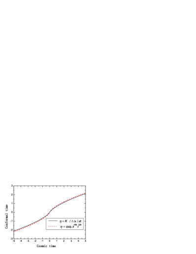
Figure 1: The relation between the conformal time $\eta$ and the cosmic time $t$. The solid line is $\eta=\int(1/a)dt$, and the dash line is $\eta=(3/2)\mathcal{A}^{-1/6}t^{2/3}$.

Fig.1 show that $|\eta|=(3/2)\mathcal{A}^{-1/6}t^{2/3}$ is a good approximation for $\eta=\int(1/a)dt$. The most straightforward way is to insert this approximate relation to Eq.(33). However, this relation is only a asymptotic behavior corresponding to the case of $|t|\rightarrow\infty$, not the behavior on all time. So we should consider the asymptotic behavior of $\bar{p}(\eta)$.

Under the approximation of Eq.(39), the asymptotic behavior of $\bar{p}(\eta)$ is

$$\bar{p}(\eta)=\left\{\begin{aligned} \frac{2}{3}\mathcal{A}^{1/2}|\eta|,\ \ \ |t|\rightarrow\infty,\ \ \ (far\ from\ the\ bounce)\\ \bar{p}_{min},\ \ |t|\rightarrow 0.\ \ \ \ \ \ \ \ \ \ \ (near\ the\ bounce)\end{aligned}\right.$$ (40)

Now, we construct a function of $\bar{p}(\eta)$ approximately. The approximate function should satisfy the asymptotic behavior of $\bar{p}(\eta)$. One class of such functions are

$$\bar{p}(\eta)=\left[\bar{p}_{min}^{n}+\left(\frac{2}{3}\right)^{n}\mathcal{A}^{n/2}|\eta|^{n}\right]^{1/n},$$ (41)

where $n$ is a natural number.

One can find that if $n$ is even, there will not be an absolute value like $|\eta|$ appeared in the equation. So, from now on we set $n=2$. There is another reason to choose $n=2$ that only $n=2$ can lead to a evolution equation of the Bardeen potential which have analytical solution (see Eq.(47)).

So we set the approximate function of $\bar{p}(\eta)$ is

$$\bar{p}(\eta)=\left(\bar{p}_{min}^{2}+\mathbb{A}\eta^{2}\right)^{1/2},$$ (42)

where $\mathbb{A}=\frac{4}{9}\mathcal{A}$. Eq.(42) is different with Eq.(33). Equation (33) is exact evolution of $\bar{p}$ but Eq.(42) is a approximation of Eq.(33).

Under the condition of $V(\bar{\varphi})=0$, we have $P_{s}=\rho_{s}$, so $\Upsilon=1$. From Eqs.(14), (15) and (21) we can obtain

$$\beta = 3(\mathbb{H}^{2}-\mathfrak{S}_{1}),$$ (43)

$$\mathfrak{S}_{2} = 2\mathbb{H}^{2}-2\mathfrak{S}_{1}+\mathbb{H}^{\prime}.$$ (44)

Using these equations and Eq.(LABEL:e29) one can get

$$\Phi^{\prime\prime}_{k}+\left(8\mathbb{H}+\frac{\mathbb{H}^{\prime}}{\mathbb{H}}-2\frac{\mathfrak{S}_{1}}{\mathbb{H}}\right)\Phi^{\prime}_{k}+(k^{2}+4\mathfrak{S}_{1})\Phi_{k}=0.$$ (45)

Using Eq.(42) and Eq.(45), we can discuss the behaviors of the evolution equation of the Bardeen potential in the following cases.

III.1.1 Near the bounce

Near the bounce point, $|\eta|\rightarrow 0$, and the leading order of the coefficients of evolution equation are

$$8\mathbb{H}+\frac{\mathbb{H}^{\prime}}{\mathbb{H}}-2\frac{\mathfrak{S}_{1}}{\mathbb{H}}\approx\left(1+\frac{2p_{\bar{\varphi}}^{2}l_{p}^{2}}{\mathbb{A}}\right)\frac{1}{\eta},\quad 4\mathfrak{S}_{1}\approx-\frac{2p_{\bar{\varphi}}^{2}}{l_{p}^{2}}.$$ (46)

And the evolution equation changes to

$$\Phi^{\prime\prime}_{k}+\left(1+\frac{2p_{\bar{\varphi}}^{2}l_{p}^{2}}{\mathbb{A}}\right)\frac{1}{\eta}\Phi^{\prime}_{k}+\left(k^{2}-\frac{2p_{\bar{\varphi}}^{2}}{l_{p}^{2}}\right)\Phi_{k}=0.$$ (47)

and the solutions of Eq.(47) is

$$\Phi_{k}(\eta)=\eta^{\nu}[C_{1}Z_{\nu}(\mathcal{K}\eta)+C_{2}Z_{-\nu}(\mathcal{K}\eta)]$$ (48)

where

$$\mathcal{K}=\sqrt{k^{2}-\frac{2p_{\varphi}^{2}}{l_{p}^{2}}},\ \ \ \nu=-\frac{p_{\bar{\varphi}}^{2}l_{p}^{2}}{\mathbb{A}}.$$ (49)

and $Z_{\nu}$ is Bessel function, $C_{1}$, $C_{2}$ are arbitrary constants.

The leading order of this solution is

$$\Phi_{k}(\eta)\approx\Phi_{(1)}+\Phi_{(2)}\eta^{2\nu},$$ (50)

where $\Phi_{(1)}$ and $\Phi_{(2)}$ are constants which related to $k$.

One can found that, $\nu<0$, and the second term in Eq.(50) is divergence. But we can choose the arbitrary constant $C_{2}=0$, which means $\Phi_{(2)}=0$. Thus we can obtain a convergence solution of scalar perturbations near the bounce.

III.1.2 NEC transition problem

In our model, the point of NEC transition is obtained form $\beta=0$. When $V(\bar{\varphi})=0$, the $\beta$ is Eq.(43).

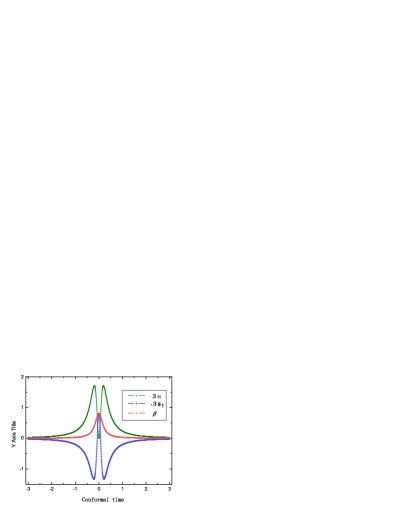
Figure 2: The evolutions of $\mathbb{H}$, $-\mathfrak{S}_{1}$ and $\beta$ near the bounce point.

From the Fig.2, we can see that $\beta$ is always positive in our model. So there is no NEC transition. And then, there is not the problem of the divergence near the point of NEC transition.

In GR, if the matter always satisfies NEC, there will be no bounce. The reason is that the GR bounce is led by some exotic matter which violates the NEC. However, in LQC, the bounce is originated in the discrete spacetime geometry. It is a quantum effect of spacetime. So, even if the matter never violates the NEC, there is also a bounce phase.

III.2 Toy model

In this subsection, we extend our discussion slightly, and consider a toy model which was introduced in r98 ; r99 . In this model, the universe is radiation-dominated in the asymptotic past and future. In other words, the asymptotic behavior of $a(\eta)$ should be $a\propto\eta$ or $\bar{p}\propto\eta^{2}$. So we assume that there are some $V(\bar{\varphi})$ that can make the form of $\bar{p}(\eta)$ as

$$\bar{p}(\eta)=(b^{m}+\alpha\eta^{2m})^{1/m},$$ (51)

where $b$, $\alpha$ are constants, and $b>0,m>1$.

III.2.1 Near the bounce

Under the assumption of Eq.(51), we can obtain the evolution equation of the perturbation near the bounce point from Eq.(LABEL:e29)

$$\Phi_{k}^{\prime\prime} + \left[1-\frac{2m-2}{\sqrt{b}}-(2m-1)(\sqrt{b}+b)\right]\frac{1}{\eta}\Phi_{k}^{\prime}$$ (52)

$$- \frac{b^{(2m-1)/2}(2m-2)(1+\sqrt{b})}{3\alpha}\frac{k^{2}}{\eta^{2m}}\Phi_{k}=0.$$

In fact, Eq.(52) is only accurate to its leading order. We can obtain the following analytical solution

$$\Phi_{k}(\eta)=\eta^{(1-m)\nu}[\Phi_{(1)}\mathcal{Z}_{\nu}(\kappa\eta^{1-m})+\Phi_{(2)}\mathcal{Z}_{-\nu}(\kappa\eta^{1-m})],$$ (53)

where $\mathcal{Z}_{\nu}$ is the Bessel function, $\Phi_{(1)}$ and $\Phi_{(2)}$ are constants, and

$$\nu = \frac{1}{1-m}\left[\frac{m-1}{\sqrt{b}}+\left(n-\frac{1}{2}\right)(\sqrt{b}+b)\right],$$ (54)

$$\kappa = \frac{ik}{m-1}\sqrt{\frac{b^{(2m-1)/2}(2m-2)(1+\sqrt{b})}{3\alpha}}.$$ (55)

The leading order of Eq.(53) is

$$\Phi_{k}(\eta)\approx\kappa^{\nu}[\Phi_{(1)}+\Phi_{(2)}\eta^{2(1-m)\nu}].$$ (56)

Because $2(1-m)\nu=(2m-2)/\sqrt{b}+(m-1)(\sqrt{b}+b)>0$, so the behavior of the perturbation near the bounce point is good.

III.2.2 NEC transition problem

Near the bounce point, the leading order of $\beta$ is

$$\beta\approx-\frac{\alpha(2m-1)(\sqrt{b}+b)}{b^{m}}\eta^{2m-2}<0.$$ (57)

So, there must be a time point corresponding to $\beta=0$. To get this point, we consider the next order of $\beta$

$$\beta\approx - \frac{\alpha(2m-1)(\sqrt{b}+b)}{b^{m}}\eta^{2m-2}$$

$$+ \frac{\alpha^{2}[(2m-1)(4m-1)(\sqrt{b}+b)+b]}{2mb^{2m}}\eta^{4m-2}.$$

Near the bounce point, the leading order term is $\eta^{2m-2}$ term, so $\beta<0$. When $|\eta|$ get larger, the leading order term will be $\eta^{4m-2}$, so $\beta>0$. The transition point is $\beta=0$, it leads to a transition point

$$\eta_{0}\approx\pm\left[\frac{b^{m}}{\alpha(4m-1)}\right]^{\frac{1}{2m}},$$ (59)

$\eta_{0}$ denotes the transition time.

When we discuss the perturbation near the $\eta_{0}$, we can shift the origin of the time such that $\eta_{0}=0$. If we do that, the function of $\bar{p}(\eta)$ will be

$$\bar{p}(\eta)=[b^{m}+\alpha(\eta+\eta_{0})^{2m}]^{1/m}.$$ (60)

Near the point $\eta_{0}$, $\beta\approx 0$ and $\Upsilon\approx-2/3$. Moreover, from the definition of $\beta$ and $\beta=0$, we have $\mathfrak{S}_{2}=\mathfrak{S}_{1}-\mathbb{H}^{2}+\mathbb{H}^{\prime}$. Thus, Eq.(LABEL:e29) changes to

$$\Phi_{k}^{\prime\prime}+\frac{\mathfrak{S}_{1}+\mathbb{H}^{\prime}}{\mathbb{H}}\Phi_{k}^{\prime}+\left(-\frac{2}{3}k^{2}+5\mathfrak{S}_{1}-\frac{5}{3}\mathbb{H}^{2}+\frac{8}{3}\mathbb{H}^{\prime}\right)\Phi_{k}=0.$$ (61)

Near the $\eta_{0}$, the leading order of this equation is

$$\Phi_{k}^{\prime\prime}+L_{1}\Phi_{k}^{\prime}+\left(-\frac{2}{3}k^{2}+L_{2}\right)\Phi_{k}=0,$$ (62)

where $L_{1}$ and $L_{2}$ are constants which can be related to $m,\Delta$ etc. The solution of this equation is

$$\Phi_{k}=\Phi_{(1)}\exp\left[-\frac{1}{2}(L_{1}+\hat{k})\eta\right]+\Phi_{(2)}\exp\left[-\frac{1}{2}(L_{1}-\hat{k})\eta\right],$$ (63)

where $\Phi_{(1)}$ and $\Phi_{(2)}$ are constants again and

$$\hat{k}=\sqrt{4\left(\frac{2}{3}k^{2}-L_{2}\right)+L_{1}^{2}}.$$ (64)

Near the NEC transition point, we can see a convergence behavior of the perturbation.

IV vector perturbation with holonomy corrections

In the most of research on perturbations of cosmology, a lot of attention have been focused on the scalar and the tensor mode. The reason is that the vector mode will decay quickly in expanding phase of universe.

However, in the pre-bounce phase of the bounce models, the universe undergoes a contracting. It is shown that, in contrast with the expanding phase, the vector mode will exhibit a growing behavior r97 . The unlimited growth of the perturbation will breakdown the perturbation theory. So, it is necessary to check the behaviors of the vector mode near the bounce.

The effective linearized equations of vector mode with holonomy corrections have been given in r96 (in Newton gauge):

$$-\frac{1}{2a^{2}}\nabla^{2}{\cal S}^{i}=(8\pi G)^{2}(\rho+P){\cal V}^{i},$$ (65)

$$-\frac{1}{2}\partial_{\eta}\left({\cal S}_{~{},j}^{i}+{\cal S}_{~{},i}^{j}\right)-\frac{\bar{\mathfrak{K}}}{2a}\left(1+\left[\frac{\sin(2\tilde{\mu}\gamma\bar{\mathfrak{K}})}{2\gamma\tilde{\mu}\bar{\mathfrak{K}}}\right]\right)\left({\cal S}_{~{},j}^{i}+{\cal S}_{~{},i}^{j}\right)+{\cal{G}}_{(i}^{~{}~{}j)}=(8\pi G)^{2}\bar{p}\left(\Pi_{~{},j}^{i}+\Pi_{~{},i}^{j}\right),$$ (66)

where $\mathcal{S}^{i}$ and $\mathcal{V}^{i}$ are the metric perturbation and the 4-velocity perturbation of the vector mode respectively, $\Pi^{i}$ is the anisotropic stress, and ${\cal{G}}_{i}^{~{}j}$ is the anomaly term r96 . To have a consistent set of the evolution equations, we require the anomaly term to vanish i.e. ${\cal{G}}_{i}^{~{}j}=0$.

From Eq.(65), one can obtain a relation between $\mathcal{V}$ and $\mathcal{S}$ in Fourier mode of $k$:

$$\mathcal{V}_{k}^{i}=\frac{1}{2(8\pi G)^{2}\bar{p}(\rho+P)}k^{2}\mathcal{S}_{k}^{i}.$$ (67)

If we do not take into account the anisotropic of perturbations, the Eq.(66) will be:

$$\left[-\frac{1}{2}\partial_{\eta}-\frac{\bar{\mathfrak{K}}}{2a}\left(1+\left[\frac{\sin(2\tilde{\mu}\gamma\bar{\mathfrak{K}})}{2\gamma\tilde{\mu}\bar{\mathfrak{K}}}\right]\right)\right]\left(\mathcal{S}^{i}_{~{},j}+\mathcal{S}^{j}_{~{},i}\right)=0,$$ (68)

and the equation of the Fourier mode $k$ is

$$\frac{\partial}{\partial\eta}\mathcal{S}^{i}_{k}+\frac{\bar{\mathfrak{K}}}{a}\left(1+\left[\frac{\sin(2\tilde{\mu}\gamma\bar{\mathfrak{K}})}{2\gamma\tilde{\mu}\bar{\mathfrak{K}}}\right]\right)\mathcal{S}^{i}_{k}=0.$$ (69)

We will solve the Eq.(69) in two models which is the same as the Sec. III.

IV.1 Massless scalar field

For the same massless scalar field model discussed in Sec. III.1, the evolution of the scale factor is Eq.(42), and the Eq.(69) changes into

$$\frac{\partial}{\partial\eta}\mathcal{S}^{i}_{k}+\frac{\mathbb{A}^{2}}{\bar{p}_{min}}\eta\mathcal{S}^{i}_{k}=0.$$ (70)

We only consider the leading term and thus

$$\mathcal{S}^{i}_{k}\propto\exp\left(-\frac{\mathbb{A}^{2}}{2\bar{p}_{min}}\eta^{2}\right)$$ (71)

We can see that, even though the vector mode is growing when the universe contracting to bounce, there is a maximum at the point of the bounce. It means that the vector mode should not growing unlimited.

As pointed out in r97 that, only the combination $(\rho+P)\mathcal{V}^{i}$ appears in the energy momentum tensor; therefore it is this combination that could in principle be observable and may thus be called physically relevant.

From Eq.(67), we can obtain:

$$(\rho+P)\mathcal{V}^{i}_{k}\propto\frac{\exp\left(-\frac{\mathbb{A}^{2}}{2\bar{p}_{min}}\eta^{2}\right)}{(\bar{p}_{min}^{2}+\mathbb{A}\eta^{2})^{1/2}}$$ (72)

This also have a maximum at the point of bounce and it inversely proportional with $\bar{p}_{min}=a_{bounce}^{2}$.

IV.2 Toy model

For the same toy model discussed in Sec. III.2, the form of $\bar{p}(\eta)$ is taken as Eq.(51) and the Eq.(69) approximating into the leading order becomes

$$\frac{\partial}{\partial\eta}\mathcal{S}^{i}_{k}+\frac{2\alpha}{b^{m}}\eta^{2m-1}\mathcal{S}^{i}_{k}=0.$$ (73)

We can obtain

$$\mathcal{S}^{i}_{k}\propto\exp\left(-\frac{\alpha}{mb^{m}}\eta^{2m}\right).$$ (74)

This means that the limited growing is the same as Eq.(71), and we also have

$$(\rho+P)\mathcal{V}^{i}_{k}\propto\frac{\exp\left(-\frac{\alpha}{mb^{m}}\eta^{2m}\right)}{(b^{m}+\alpha\eta^{2m})^{1/m}}.$$ (75)

We find that, the maximum of $(\rho+P)\mathcal{V}^{i}_{k}$ is also inversely proportional with $b=a_{bounce}^{2}$. It means that the maximum of the observable quantity $(\rho+P)\mathcal{V}^{i}_{k}$ near the bounce is inversely proportional to the square of scale factor at the bounce point, and this conclusion is independent with the model.

V discussion and conclusions

In this paper, we examined the behaviors of the scalar and the vector perturbations in the bounce phase of the effective theory of LQC. Differing from the bounce model in r3 , the scalar perturbations in our model is not divergence near both the bounce point and the NEC transition point. Another conclusion is that the vector mode of perturbations have maximum at the bounce point, and this maximum is inversely proportional to the square scale factor at the bounce point.

In the model of GR bounce, the emergence of bounce phase is rooted in the matter in the universe. According to the singularity theorems r2 ; r16 , if one requires the matter satisfies the energy conditions, the universe can be emerged from an initial singularity. However, there is no evidence that the exotic matter which violates the NEC does not exist. So one can choose some exotic matter to make the universe to experience a bounce. It is also because of this, the behavior of the bounce and the perturbation near the bounce point is decided by some exotic matter which have been chosen. Therefore, we can select the matter carefully to make the behavior of perturbation near the bounce have good performance like in r12 ; r13 ; r14 . But too much artificial factors will make the physics of the model unnatural.

On the other hand, the LQC bounce is originated in the discrete spacetime geometry. Just like the model in Sec. III.1, even if the matter satisfies the NEC, there is also a bounce phase. So the behavior of the bounce is decided by the effects of discrete spacetime geometry. From the analysis in Sec. III.1 and III.2, one can find that, the effects of discrete spacetime geometry lead to the convergence of the Bardeen potential.

One should note that, our discussion is in the framework of the effective theory of LQC, so we find that this effective theory reflects the nature of quantum spacetime geometry effectively. Moreover, from the discussion of this paper, we also can obtain the conclusion that the existence of LQC bounce is reasonable, it do not lead to unbounded growth of the perturbation.

References

(1)Borde A and Vilenkin A, Int. J. Mod. Phys. D 5 813
(1996).
(2)Tolman R C, Phys. Rev. 38 1758
(1996).
(3)Durrer R and Laukenmann J, Class. Quantum Grav. 13
1069 (1996).
(4)Elbaz E, Novello M, Salim J M and Oliverira L A R, Int. J. Mod. Phys. D 1
641 (1993).
(5)Patrick Peter and Nelson Pinto-Neto, Phys. Rev. D 65
023513 (2001).
(6)Patrick Peter, Nelson Pinto-Neto and Diego A Gonzalez, J. Cosmology and Astroparticle Phys. 12
003 (2003).
(7)Patrick Peter and Nelson Pinto-Neto, Phys. Rev. D 66
063509 (2002).
(8)Fabio Finelli, Patrick Peter and Nelson Pinto-Neto, Phys. Rev. D 77
103508 (2008).
(9)T. J. Battefeld and R. Brandenberger,
Phys. Rev. D 70, 121302(R) (2004)
(10)T.Thiemann,Introduction to Modern Canaoical Quantum General Relativity (Cambridge University Press, Cambridge, England,
2007).
(11)C.Rovell,Quantum Gravity (Cambridge University Press, Cambridge, England,
2004).
(12)A.Ashtekar and J.Lewandowski, Class. Quantum Grav. 21,
R53 (2004).