Resonant enhancement of ultracold photoassociation rate by electric field induced anisotropic interaction

Abstract

We study the effects of a static electric field on the photoassociation of a heteronuclear atom-pair into a polar molecule. The interaction of permanent dipole moment with a static electric field largely affects the ground state continuum wave function of the atom-pair at short separations where photoassociation transitions occur according to Franck-Condon principle. Electric field induced anisotropic interaction between two heteronuclear ground state atoms leads to scattering resonances at some specific electric fields. Near such resonances the amplitude of scattering wave function at short separation increases by several orders of magnitude. As a result, photoaasociation rate is enhanced by several orders of magnitude near the resonances. We discuss in detail electric field modified atom-atom scattering properties and resonances. We calculate photoassociation rate that shows giant enhancement due to electric field tunable anisotropic resonances. We present selected results among which particularly important are the excitations of higher rotational levels in ultracold photoassociation due to electric field tunable resonances.

1 Introduction

Research interest in the field of cold molecules has witnessed a tremendous growth in recent times. The possibility to investigate molecular behaviour at low temperatures motivates physicists and chemists from diverse backgrounds to study cold and dense molecular gases. Certainly, this development is inspired by the great success in the closely related field of cold atoms. Molecules can have properties which are not available with atoms, for instance a hetero-nuclear molecule can possess permanent electric dipole moment. While the rich internal structure of molecules possesses new challenges for cooling and trapping them, the potential applications of cold molecules are remarkable. This is especially true for ultracold polar molecules which allow for a wealth of interesting studies. The interaction of permanent dipoles with an external electric field provides a tool to manipulate physical processes taking place in the ultracold regime. Several quantum computation devices have been proposed based on the interaction of the heteronuclear dimers with external electric fields [1, 2]. External electric fields can also alter the internal rovibrational structure and dynamics of heteronuclear molecules [3, 4, 5]. The orientation, angular motion, hybridization, and changes in the transition rates and lifetimes of the rovibrationally excited state of a LiCs molecule in a strong static electric field have been theoretically studied [6, 7]. Electric field is used to enhance the interaction between Li and Cs atoms in an ultracold collision [8, 9]. This enhancement is due to the interaction of the instantaneous dipole moment of the heteronuclear collision complex with the static electric field. The interaction of a heteronuclear pair of atoms with an electric field can couple states of different angular momenta in the electronic ground continuum of the pair leading to resonances in an ultracold collision.

Our purpose here is to utilize the static electric field induced scattering resonances to influence free-bound photoassociation (PA) [10] process of molecule formation. PA of ultracold atoms via the interaction with an electromagnetic field has become a standard technique to produce cold and ultracold molecules. The experimental techniques previously used for the formation of homonuclear molecules have been extended to heteronuclear alkali-metal dimers. Several experimental groups have reported the photoassociative formation of ultracold alkali-metal dimers , such as NaCs [11], KRb [12, 13, 14], RbCs [15, 16] and LiCS [17] in their electronic ground states. The effect of a static electric field on the formation of heteronuclear molecules in their electronic ground state via one-photon stimulated emmision from ground continuum has been theoretically studied [18].

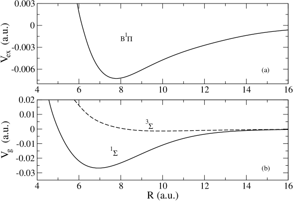
Figure 1: Adiabatic Born-Oppenheimer potentials of LiCs without hyperfine interaction for excited (a) and ground (b) states. The ground state asymptotically corresponds to both Li and Cs atoms in electronic S state while excited state corresponds to Li in S state and Cs in P state.

Here we investigate the effect of a static electric field on the photoassociation process of a heteronuclear atom pair to produce molecules in an excited electronic state. Since an electric field can couple different angular momentum states (partial waves), we need to investigate anisotropic scattering at low energy. Taking LiCs molecule as a prototype, we first present a detailed investigation of low-energy anisotropic atomic collision in the presence of a static electric field. We have used Numerov-Cooley algorithm-based multichannel scattering techniques and found several anisotropic resonant structures in the scattering cross-sections of ⁷Li + ¹³³Cs collision. Although the effects of a magnetic Feshbach resonance [19] on PA has been recently studied both experimentally [20, 21] and theoretically [22, 23, 24, 25, 26], to the best of our knowledge, the effects of electric field induced anisotropic resonances on PA into excited molecular levels have not been yet studied. One notable feature of the influence of these anisotropic resonances on PA is the occurrence of higher rotational excitations in excited molecule. This follows from the large modification of two-atom continuum wave functions for higher partial waves. Owing to the strong spatial dependence of permanent dipole moment at short separations, the interaction of a static electric field with the permanent dipole moment of a heteronuclear atom-pair leads to large enhancement of continuum wave functions at short separations, near electric fields at which anisotropic resonances occur.

This paper is organised as follows: First, we briefly discuss how an external static electric field modifies the effective interaction potential between two heteronuclear collision pair. In section 2, we present mathemetical formulation of the problem with an emphasis on anisotropic scattering. The effects of an external static electric field on the ground state scattering of ⁷Li + ¹³³Cs are discussed in section 3. In section 4, we discuss the effects of static electric field-induced anisotropic interaction on PA rate and present our main results. Finally we summarize and come to the conclusion in section 5.

2 Formulation

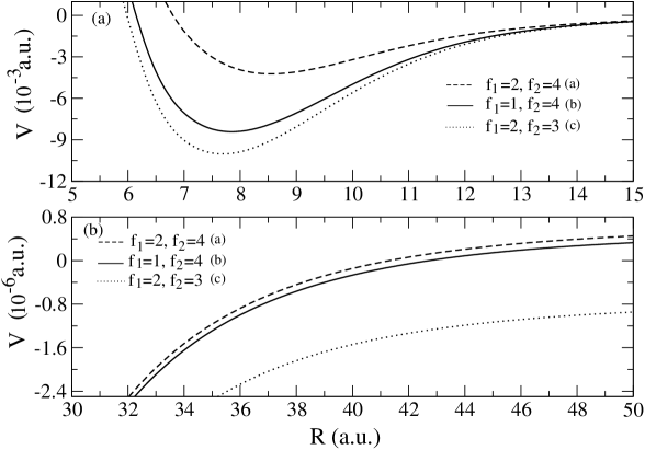
Figure 2: The potentials V(R) of LiCs in different diabatic hyperfine channels as a function of internuclear distance R are plotted. Panel (a) shows the short range and panel (b) shows the long range part of the potentials. $f_{1}$ and $f_{2}$ are the hyperfine quantum numbers of ⁷Li and ¹³³Cs, respectively (See Tabel-I in the text).

The dynamics of Li-Cs collision in the presence of an electric field is effectively described by the radial Hamiltonian

$$\hat{H}_{R}=-\frac{1}{2\mu R}\frac{\partial^{2}}{\partial R^{2}}R+\frac{\hat{L}^{2}(\theta,\phi)}{2\mu R^{2}}+\hat{V}_{c}(R)+\hat{V}_{hf}+\hat{V}_{\cal E}$$ (1)

where $\mu={m_{1}m_{2}}/{(m_{1}+m_{2})}$ is the reduced mass of two atoms ⁷Li and ¹³³Cs with masses $m_{1}$ and $m_{2}$ respectively, R is the interatomic distance, $\hat{L}^{2}$ is the rotational angular momentum of the collision complex and the angles $\theta$ and $\phi$ specify the orientation of the interatomic axis in the space fixed coordinate frame. The electronic interaction potential can be represented as

$$\hat{V}_{c}(R)=\sum_{S}\sum_{M_{S}}\mid SM_{S}\rangle V_{S}(R)\langle SM_{S}\mid$$ (2)

where S is the total electronic spin of the two atoms and $M_{S}$ is the projection of S on the Z-axis. $V_{S}(R)$ represents the adiabatic interaction potential of the molecule in the spin state S. The ground state $V_{g}(R)$ and the excited state $V_{ex}(R)$ potentials as shown in figure 1, are taken from [27] and [28], respectively. This interaction is therefore diagonal in the adiabatic basis $\mid IM_{I};SM_{S}\rangle$,

$$\langle S^{\prime}M_{S}^{\prime};I^{\prime}M_{I}^{\prime}\mid\hat{V}_{c}(R)\mid SM_{S};IM_{I}\rangle=\delta_{I,I^{\prime}}\delta_{M_{I},M_{I}^{\prime}}\delta_{S,S^{\prime}}\delta_{M_{S},M_{S}^{\prime}}V_{S}(R)$$ (3)

where $\vec{S}=\vec{s_{1}}+\vec{s_{2}}$ and $\vec{I}=\vec{i_{1}}+\vec{i_{2}}$, $\vec{s_{1}}$ and $\vec{s_{2}}$ are the electronic spins while $\vec{i_{1}}$ and $\vec{i_{2}}$ are the nuclear spins of the Li and Cs atoms, respectively. The total hyperfine Hamiltonian $\hat{V}_{hf}$ for the collision complex can be written as a sum of the two atomic hyperfine Hamiltonian

$$\hat{V}_{hf}=\sum_{j=1}^{2}\frac{a_{hf}^{(j)}}{\hbar^{2}}\vec{s}_{j}.\vec{i}_{j}=\sum_{j=1}^{2}\frac{a_{hf}^{(j)}}{2\hbar^{2}}(\vec{f}_{j}^{2}-\vec{s}_{j}^{2}-\vec{i}_{j}^{2})$$ (4)

where $\vec{f}_{j}=\vec{s}_{j}+\vec{i}_{j}$ is the total spin and $a_{hf}^{(j)}$ is the hyperfine constant of atom $j$ which is 402.00 MHz for ⁷Li and 2298.25 MHz for ¹³³Cs [29]. This hyperfine interaction is diagonal in the atomic or diabatic or long range basis $\mid\ell,f,f_{1},f_{2}\rangle$ in which $\hat{V}_{c}(R)$ can be expressed as,

$$\langle(f_{1}^{\prime}f_{2}^{\prime})f^{\prime}m_{f^{\prime}}\ell^{\prime}m_{\ell^{\prime}}\mid\hat{V}_{c}(R)\mid(f_{1}f_{2})fm_{f}\ell m_{\ell}\rangle$$

$$=\sum_{S^{\prime}M_{S^{\prime}},I^{\prime}M_{I^{\prime}}}V_{S}\langle SM_{S};IM_{I};\ell m_{\ell}\mid(f_{1}f_{2})fm_{f}\ell m_{\ell}\rangle$$

$$\times\langle(f_{1}^{\prime}f_{2}^{\prime})f^{\prime}m_{f^{\prime}};\ell^{\prime}m_{\ell^{\prime}}\mid S^{\prime}M_{S^{\prime}};I^{\prime}M_{I^{\prime}};\ell^{\prime}m_{\ell^{\prime}}\rangle.$$ (5)

The transformation from coupled hyperfine representation to short range representation is given by

$$\langle SM_{S};IM_{I};\ell^{\prime}m_{\ell^{\prime}}\mid(f_{1}f_{2})fm_{f};\ell m_{\ell}\rangle$$

$$=\delta_{\ell\ell^{\prime}}\delta_{m_{\ell}m_{\ell^{\prime}}}\langle SM_{S};IM_{I}\mid fm_{f}\rangle\sqrt{(2f_{1}+1)(2f_{2}+1)(2S+1)(2I+1)}$$

$$\times\left\{\begin{array}[]{ccc}s_{1}&i_{1}&f_{1}\\ s_{2}&i_{2}&f_{2}\\ S&I&f\end{array}\right\}$$ (9)

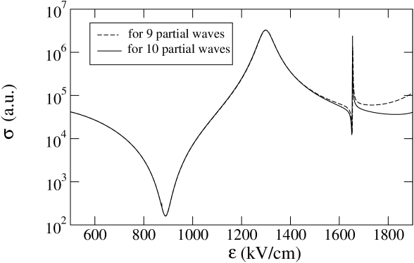
Figure 3: Total elastic cross-section $\sigma$ in a.u. vs electric field $\cal E$ in kV/cm is plotted for different total number of partial waves to show the convergence of the first resonance point at $\cal E$ = 1298 kV/cm.

Table 1: Three different hyperfine channels of ⁷Li and ¹³³Cs.

Channel index	$f_{1}$(7Li)	$f_{2}$(133Cs)	$f$
a	2	4	5
b	1	4	5
c	2	3	5

where $\langle SM_{S};IM_{I}\mid fm_{f}\rangle$ is Clebsch Gordon coefficient and the quantity in curly braket is 9j-symbol. The hyperfine Hamiltonian can only couples channels with the same total angular momentum projection $m_{f}=m_{f1}+m_{f2}=M_{S}+M_{I}$ where $m_{f1}$, $m_{f2}$, $M_{S}$ and $M_{I}$ are the projections of $f_{1}$, $f_{2}$, S and I respectively. For ⁷Li, $i_{1}=3/2$ and for ¹³³Cs, $i_{2}=7/2$ (both with $s_{1}$ = $s_{2}$ = 1/2). Since $m_{f}$ takes values from -6 to +6, the total degeneracy of the atom pair is 128. However, atoms mainly collide on the Li($2{{}^{2}{S}_{{1}/{2}}},f_{1}=2$) + Cs($6{{}^{2}{S}_{{1}/{2}}},f_{2}=3$) channel, and thus only 35 degenerate entrance channels have to be considered. For $f=5$, three collisional channels are possible as given in Table 1. The potentials of these three channels are shown in figure 2 . We consider a single asymptotic hyperfine channel (c) with $f_{1}=2,f_{2}=3$ since the difference in energy of this channel from the other two channels is large enough compared to collision energy at ultracold temperatures. Thus we can approximate our calculation as a single channel with $f_{1}=2,f_{2}=3$. The operator $\hat{V}_{\cal E}(R)$ describes the interaction of the atoms with an external electric field. It can be written in the form

$$\hat{V}_{\cal E}(R)=-\cal E\rm cos\theta\sum_{S}\sum_{M_{S}}\mid SM_{S}\rangle d_{S}(R)\langle SM_{S}\mid$$ (10)

where d_S(R) denotes the dipole moment functions of LiCs in the different spin states and $\cal E$ the electric field magnitude. Li and Krems [9] have given an analytical expression for this dipole moment function approximating the numerical data computed by Aymar and Dulieu [30]. This analytical expression is given by

$$d_{S}(R)=D\exp\left[-\alpha(R-R_{e})^{2}\right],$$ (11)

with the parameters $R_{e}$ = 7.7 $a_{0}$, $\alpha$ = 0.1 $a_{0}^{-2}$, and $D=6$ Debye for the singlet state and $D=0.5$ Debye for the triplet state (where $a_{0}$ = Bohr radius ). The matrix element of $\hat{V}_{\cal E}(R)$ are evaluated using the expressions

$$\langle\ell m_{\ell}\mid\cos\theta\mid\ell^{\prime}m_{\ell^{\prime}}\rangle = \delta{m_{\ell}m_{\ell^{\prime}}}(-1)^{m_{\ell}}\left(\!\!\begin{array}[]{ccc}\ell&1&\ell^{\prime}\\ -m_{\ell}&0&m_{\ell^{\prime}}\\ \end{array}\!\!\right)\left(\!\!\begin{array}[]{ccc}\ell&1&\ell^{\prime}\\ 0&0&0\\ \end{array}\!\!\right)$$

$$\times \left[(2\ell+1)(2\ell^{\prime}+1)\right]^{{1}/{2}}$$

and

$$\langle SM_{s}\mid\left(\sum_{S^{\prime\prime}}\sum_{M_{S}^{\prime\prime}}\mid S^{\prime\prime}M_{S}^{\prime\prime}\rangle d_{S^{\prime\prime}}\langle S^{\prime\prime}M_{S}^{\prime\prime}\mid\right)\mid S^{\prime}M_{S}^{\prime}\rangle=d_{S}\delta_{SS^{\prime}}\delta_{M_{S}M_{S^{\prime}}}$$ (17)

where $\langle\vec{R}\mid\ell,m_{\ell}\rangle=Y_{\ell m_{\ell}}(\hat{R})$. Due to the symmetry of the z-component of the angular momentum, the matrix element $\langle\ell m_{\ell}\mid\cos\theta\mid\ell^{\prime}m_{\ell^{\prime}}\rangle$ exists only if $\ell-\ell^{\prime}=\pm 1$ and $m_{\ell}=m_{\ell^{\prime}}$. Therefore electric field can couple even and odd parity channels to each other but not to themselves.

The scattering wave function can be expressed as

$$\Psi(\vec{R})=\frac{1}{R}\sum_{\ell m_{\ell}}\psi_{\ell,m_{\ell}}(R)Y_{\ell m_{\ell}}^{*}(\hat{k})Y_{\ell m_{\ell}}(\hat{R})$$ (18)

which has the asymptotic form

$$R\Psi(\vec{R})\sim R\exp(i\vec{k}.\vec{R})+f_{\vec{k},\vec{k}^{\prime}}\exp(ikR),$$ (19)

where $\vec{k}$ and $\vec{k}^{\prime}$ are the incident and the scattered momentum, respectively. The on-shell elastic scattering is then described by $f_{\vec{k},\vec{k}^{\prime}}$, with the scattered momentum $\vec{k}^{\prime}=k\hat{R}$. Expanding the scattering amplitude $f_{\vec{k},\vec{k}^{\prime}}$ into the complete basis $Y_{\ell m_{\ell}}$, we have

$$f_{\vec{k},\vec{k}^{\prime}}=\frac{4\pi}{k}\sum_{\ell,m_{\ell}}T_{\ell m_{\ell}}(\vec{k})Y_{\ell m_{\ell}}(\hat{R})$$ (20)

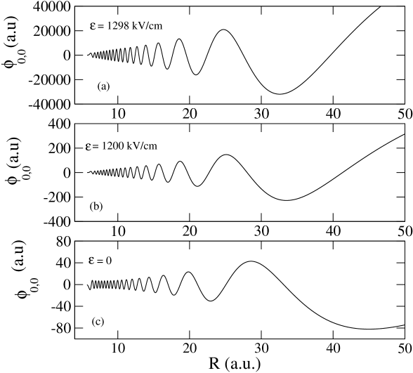
Figure 4: Energy-normalised scattering wave function $\phi_{0,0}$ (a.u.) is plotted as a function of interatomic distance R (a.u.) at the first resonant electric field $\cal E$ = 1298 kV/cm (a), $\cal E$ = 1200 kV/cm (b) and $\cal E$ = 0 (c).

where $T_{\ell m_{\ell}}$ is a T-matrix element which can also be expanded in the following form

$$\frac{1}{k}T_{\ell m_{\ell}}(\vec{k})=\sum_{\ell^{\prime},m_{\ell^{\prime}}}t_{\ell m_{\ell}}^{\ell^{\prime}m_{\ell^{\prime}}}(k)Y_{\ell^{\prime}m_{\ell^{\prime}}}(\hat{k}),$$ (21)

and

$$\exp(i\vec{k}.\vec{R})=4\pi\sum_{\ell,m_{\ell}}i^{\ell}j_{\ell}(kR)Y_{\ell m_{\ell}}^{*}(\hat{k})Y_{\ell m_{\ell}}(\hat{R}).$$ (22)

Substituting equations (13) and (15) in equation (12) we get

$$R\Psi(\vec{R}) \sim \frac{4\pi}{k}\sum_{\ell,m_{\ell}}i^{\ell}[Y_{\ell m_{\ell}}^{*}(\hat{k})\sin(kR-\ell\pi/2)+T_{\ell m_{\ell}}(\vec{k})$$ (23)

$$\times \exp(ikR-i\ell\pi/2)]Y_{\ell m_{\ell}}(\hat{R})$$

where the asymptotic form $j_{\ell}(kr)\sim\sin(kR-\ell\pi/2)/(kR)$ has been used. We get the multichannel form of the scattering equation which is given by

$$h_{\ell}\psi_{\ell m_{\ell}}(R)=\sum_{\ell^{\prime},m_{\ell^{\prime}}}i^{\ell^{\prime}-\ell}\langle\ell m_{\ell}\mid V_{\cal E}(R)\mid\ell^{\prime}m_{\ell^{\prime}}\rangle\psi_{\ell^{\prime}m_{\ell^{\prime}}},$$ (24)

where

$$h_{\ell}=-\frac{\hbar^{2}}{2\mu}\frac{d^{2}}{dR^{2}}+\frac{\hbar^{2}}{2\mu}\frac{\ell(\ell+1)}{R^{2}}+V-E.$$ (25)

$E=\hbar^{2}k^{2}/2\mu$ is the collision energy and V is the central potential for the chosen hyperfine channel. The asymptotic boundary condition on $\psi_{\ell m_{\ell}}$ can be set as

$$\psi_{\ell m_{\ell}}\sim\sin(kR-\ell\pi/2)+T_{\ell m_{\ell}}(k)\exp(ikr-i\ell\pi/2).$$ (26)

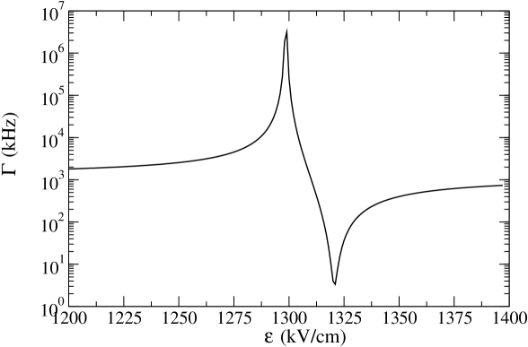
Figure 5: Plot of stimulated linewidth $\Gamma$ vs. electric field $\cal E$ at laser intensity 1W/cm².

Under the approximation of single asymptotic hyperfine channel as discussed earlier, we can write the coupled equation (17) in a matrix form in relative angular momentum $(\ell)$ basis as given by

$$\left[\left(-\frac{\hbar^{2}}{2\mu}\frac{d^{2}}{dR^{2}}+{V}\right){\bf I}+\frac{\hbar^{2}}{2\mu R^{2}}{\bf L^{2}}+{{\bf V}_{\cal E}}\right]\bf{\Phi}={E}{\bf\Phi}$$ (27)

where ${\bf I}$ is the identity matrix, $\bf L^{2}\equiv$ Diag[1(1+1), 2(2+1),……., $\ell$($\ell$+1)…..] is a diagonal matrix. The wave function $\bf\Phi$ is a matrix whose elements are given by $\phi_{\gamma^{\prime}\gamma}$ where $\gamma\equiv\ell,m_{\ell}$ and $\gamma^{\prime}\equiv\ell^{\prime},m_{\ell^{\prime}}$ are the incident and the scattered angular states respectively. Therefore the overall wave function for an incident partial wave $\gamma(\ell,m_{\ell})$ becomes

$$\psi_{\gamma=\ell,m_{\ell}}(E,R)=\sum_{\gamma^{\prime}=\ell^{\prime},m_{\ell^{\prime}},}\phi_{\gamma^{\prime}\gamma}(E,R)\mid\gamma^{\prime}\rangle.$$ (28)

By imposing the boundary conditions on the partial waves as given by equation (19), we can get the T-matrix elements, $t_{\ell m_{\ell}}^{\ell^{\prime}m_{\ell^{\prime}}}$. The total elastic cross-section is given by

$$\sigma=4\pi\sum_{\ell{\ell^{\prime}}}\sum_{m_{\ell}m_{\ell^{\prime}}}\mid t_{\ell m_{\ell}}^{\ell^{\prime}m_{\ell^{\prime}}}\mid^{2}$$ (29)

3 Ground state scattering: Electric field induced resonances

To obtain asymptotic scattering solutions, Numerov technique was adopted to numerically propagate equation (20). In the asymptotic region, the free wave function goes like

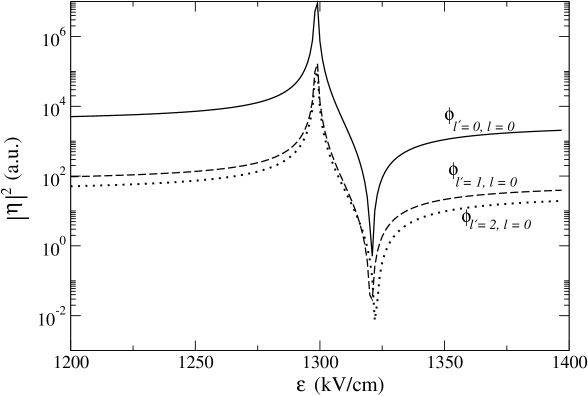
Figure 6: Square of franck-condon factor $\mid\eta\mid^{2}$ (a.u.) vs. electric field $\cal E$ (kV/cm) for transitions between the excited bound state $v=26$, $J=1$ and different scattering states $\phi_{\ell^{\prime}0,\ell 0}$ with incident partial wave $\ell=0$ and scattered partial wave $\ell^{\prime}$ = 0 (solid line), $\ell^{\prime}$ = 1 (dashed line) and $\ell^{\prime}$ = 2 (dotted line).

$$\phi_{lm}=c_{1}\sin(kR-l\pi/2)+c_{2}\cos(kR-l\pi/2).$$ (30)

We construct $S$-matrix with its elements given by $(c_{1}-ic_{2})^{-1}(c_{1}+ic_{2})$ and the $T$ matrix $(S-1)/(2i)$. In the absence of electric fields, different partial wave states of the Li-Cs collision complex are uncoupled and s-wave scattering almost entirely determines the cross-sections at ultralow kinetic energies. The interaction of pemanent dipole moment of the colliding pair of heteronuclear atoms with electric field as given by equation (7), induces coupling between different angular momentum states and may thus affect the ground state scattering wave functions. Ultracold s-wave scattering is isotropic: the probability to find the atoms after s-wave collisions does not depend on the scattering angle. The interaction with electric fields, however couples the spherically symmetric s-waves to anisotropic p-wave which in turn is coupled to d-wave, d-wave to g-wave and so on. Figure 3 shows anisotropic resonance structures in the scattering cross-section of ⁷Li + ¹³³Cs collision at 50$\mu$K energy. Typically convergent results are obtained for a minimum angular momentum of $\ell$= 9, as shown in figure 3. Larger the electric field, larger is the number of partial waves required for convergence. We get the first resonance peak near 1298 kV/cm and the second one near 1650 kV/cm. To show the effect of these resonances on PA, we have carried out PA calculations near the first resonance peak.

The permanent dipole moment function of the collision complex as given by equation (8) is typically peaked around the equilibrium distance of the diatomic molecule in the ground state and quickly decreases as the atoms separate. Due to this strong spatial dependence of permanent dipole moment at short separations, the interaction of a static electric field with the permanent dipole moment of the collision pair leads to large modification of continuum wave functions at short separations. Figure 4 demonstrates that the modification is particularly significant near the resonant electric fields. Since PA transitions take place at short separations near the outer turning point of $B^{1}\Pi$, modification of the continuum wave functions at short separations influences PA transition probability as described in the following section 4.

4 Photoassociation: Electric field effects

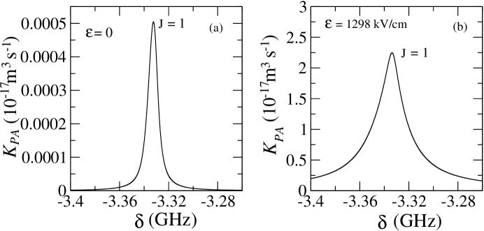
Figure 7: The photoassociation rate ${K_{PA}}$ (in unit of 10^-17cm³s^-1) is plotted as a function of atom-field detuning $\delta$ in GHz $\cal E$ = 0 (a) and at resonant electric field $\cal E$ = 1298 kV/cm.

Recently, an experiment has demonstrated the formation of ultracold bosonic ⁷Li¹³³Cs molecule in their rovibrational ground state by a two-step PA procedure [31]. For illustration of electric field effects on PA, we consider PA transition from Li($2{{}^{2}{S}_{{1}/{2}}},f_{1}=2$) + Cs($6{{}^{2}{S}_{{1}/{2}}},f_{2}=3$) continuum to the $v=26$ , $J=1$ level of $B^{1}\Pi$, near the electric fields at which anisotropic resonances occur. Photoassociation rate coefficient [32] is given by

$$K_{PA}(T,\omega_{L})=\left\langle\frac{\pi v_{rel}}{k^{2}}\sum_{\ell=0}^{\infty}(2\ell+1)\mid S_{PA}(E,\ell,\omega_{L})\mid^{2}\right\rangle$$ (31)

where $v_{rel}=\hbar k/\mu$ is the relative velocity of the two atoms, $S_{PA}(E,\ell,\omega_{L})$ is the S-matrix element for the process of loss of atoms due to PA and $\langle....\rangle$ implies an averaging over thermal velocity distribution. Assuming Maxwell-Boltzman distribution at temperature T we have,

$$K_{PA}(T,\omega_{L})=\frac{1}{hQ_{T}}\sum_{\ell=0}^{\infty}(2\ell+1)\int_{0}^{\infty}\mid S_{PA}(E,\ell,\omega_{L})\mid^{2}e^{(-E/K_{B}T)}dE$$ (32)

where

$$\mid S_{PA}(E,\ell,\omega_{L})\mid^{2}=\frac{\Gamma\gamma_{s}}{[(\delta+\frac{E-E_{v,J}}{\hbar})^{2}+((\Gamma+\gamma_{s})/2)^{2}]}.$$ (33)

Here $Q_{T}=({2\pi\mu K_{B}T}/{h^{2}})^{3/2}$ is the translational partition function and $\gamma_{s}$ is the natural linewidth of the photoassociated level. $E={\mu v_{rel}^{2}}/2$ is the relative kinetic energy of the colliding pair of atoms with reduced mass $\mu$, $E_{v,J}$ is the bound state energy and $\delta=\omega_{L}-\omega_{A}$ is the frequency offset between the laser frequency $\omega_{L}$ and atomic resonance frequency $\omega_{A}$. The stimulated linewidth $\Gamma$ is given by

$$\Gamma=\frac{\pi I}{\epsilon_{0}c}\mid\langle\phi_{v,J}\mid D_{t}(R)\mid\psi_{\gamma=l,m_{l}}(E,R)\rangle\mid^{2}$$ (34)

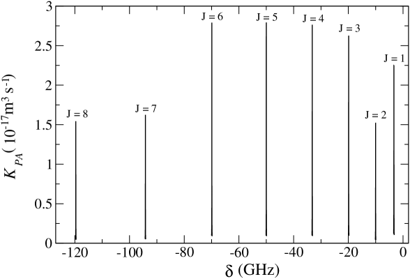
Figure 8: The photoassociation rate ${K_{PA}}$ (in unit of 10^-17cm³s^-1) is plotted as a function of atom-field detuning $\delta$ in GHz at the resonant electric field $\cal E$ = 1298 kV/cm. The rate increases for $J=3,4,5$ and $6$ rotational levels and then start decreasing for $J>7$.

where I is the intensity of the PA laser, $\epsilon_{0}$ and c are the vaccum permitivity and speed of light, respectively. $D_{t}(R)$ is the transition dipole moment. At zero electric field and for 50$\mu$K collisional energy we find $\Gamma$ = 0.315 kHz at laser intensity 1W/cm². Figure 5 demonstrates that the stimulated linewidth as a function of electric field $\cal E$ has a resonant structure with giant enhancement near the resonant electric field even at low laser intensity. This is because of large modifications of continuum wave functions at short separations. To know which components $\phi_{\gamma^{\prime},\gamma}$ of the continuum wave functions have significant contribution to such resonant enhancement of $\Gamma$, we plot square of Franck-Condon (FC) overlap integral $\mid\eta\mid^{2}$ for a few wave component $\phi_{\ell^{\prime}0,\ell 0}$ in figure 6. $\eta$ is defined by

$$\eta=\langle\phi_{v,J}\mid\psi_{\gamma=\ell,m_{\ell}}(E,R)\rangle=\langle\phi_{v,J}\mid\sum_{\gamma^{\prime}=l^{\prime},m_{l}^{\prime}}\phi_{\gamma^{\prime}\gamma}(E,R)\mid\gamma^{\prime}\rangle.$$ (35)

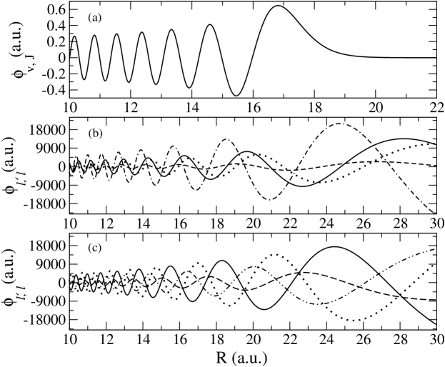
Figure 9: (a) The unit normalised bound state $\phi_{v,J}$ in a.u. In panel (b) plotted are the energy normalised scattering wave functions $\phi_{\ell^{\prime},\ell=0}$ as a function of R (a.u.) for $\ell^{\prime}$ = 0 (dashed-dotted line), $\ell^{\prime}$ = 1 (dotted line), $\ell^{\prime}$ = 2 (solid line) and $\ell^{\prime}$ = 3 (dashed line). Panel (c) shows $\phi_{\ell^{\prime},\ell=0}$ for $\ell^{\prime}$ = 4 (dotted line), $\ell^{\prime}$ = 5 (solid line), $\ell^{\prime}$ = 6 (dashed-dotted line) and $\ell^{\prime}$ = 7 (dashed line) at the resonant electric field $\cal E$ = 1298 kV/cm.

In fact, we find that a large number of partial waves significantly contribute to the resonant features. This is perhaps due to the formation of a quasibound complex inside the centrifugal barrier of a large number of partial waves which are strongly coupled among them. Figure 7 shows that ${K_{PA}}$ near the resonant electric field increases by four orders of magnitude compared to that at zero electric field. This enhancement is due to the electric field induced coupling between different partial waves. The coupling is so strong that higher rotational levels of the excited electronic state can be populated as shown in figure 8. These higher rotational excitations are not possible at ultracold temperatures in the absence of electric field. The PA rate increases for rotational levels $J=3,4,5$ and $6$ and then starts decreasing for $J>7$ as shown in figure 8. This can be understood from figure 9 which shows that the amplitude of $\phi_{\ell^{\prime}=4,\ell=0}$, $\phi_{\ell^{\prime}=5,\ell=0}$ and $\phi_{\ell^{\prime}=6,\ell=0}$,wave functions near the outer turning point of the excited molecular level are larger than $\phi_{\ell^{\prime}=1,\ell=0}$, $\phi_{\ell^{\prime}=2,\ell=0}$ and $\phi_{\ell^{\prime}=3,\ell=0}$ waves. The selection rule for free-bound transition $\left|J-|\overrightarrow{L}+\overrightarrow{S}|\right|\leq\ell^{\prime}\leq\left|J+|\overrightarrow{L}+\overrightarrow{S}|\right|$ allows the scattered partial waves $\ell^{\prime}$ = 0, 1 and 2 to be accessible for PA with J=1. Similarly, higher rotational levels $J>1$ become populated due to excitations of higher partial waves in the ground continuum through electric field induced anisotropic scattering.

The enhancement of PA rate near resonant electric fields critically depends on the outer turning point of the molecular bound state that is accessible to the PA transition. As mentioned earlier, the anisotropic resonances bring about large modification of the amplitude of continuum wave functions at relatively short separations. Now, if a prominent antinode of the modified continuum wave functions lies at a separation near the outer turning point of the bound state, then enhancement of PA rate is expected due to large FC overlap. We have chosen a particular bound state for which enhancement can be achieved. Although, in this paper we have studied enhancement of the rate of formation of excited molecular states only, the similar method of electric field induced resonances can readily be extended to enhance the formation rate of ground molecular states via one photon stimulated emission [18]. Enhancement can also be achieved using quantum interference [22, 23, 33] via laser-coupling another bound state with the continuum. In case of PA in the presence of a magnetic Feshbach resonance, a quasi-bound state embedded in the ground continuum gives rise to Fano type quantum interference [23] leading to enhancement in PA [20]. In case of heteronuclear atoms, quantum interference can be used to enhance the production of ground molecules due to the existence of permanent dipole moment. Recently, an all optical method of quantum interference scheme has been proposed for efficient production of ground state polar molecules [33]. The unique feature of the electric field induced enhancement would be the controllability of the excitations of higher rotational states.

5 Conclusion:

In conclusion, we have analysed the effects of a static electric field on the PA of a heteronuclear atom-pair. Our results show that it is possible to enhance PA rate by several orders of magnitude by tuning electric field near anisotropic resonances. Due to anisotropic nature of the interaction, a large number of partial waves in the ground continuum become strongly coupled. As a consequence, higher rotational levels can be populated in an excited dimer formed by PA at ultralow tempertures. This leads to the possibility of selectively populating higher rotational levels in ground state polar molecule by Raman-type two-color coherent PA. Furthermore it may be interesting to investigate into the effects of electric field on stimulated Raman adiabatic passage (STIRAP) from free atoms to ground state molecules. Electric field induced resonances may be coupled with multiple transition pathways to devise novel opto-electrical quantum interference schemes for efficient production of selective rovibrational molecular states.

6 Acknowledgment

One of us (Debashree Chakraborty) is grateful to CSIR, Government of India, for a support.

References

References

- [1] DeMille D. 2002 Phys. Rev. Lett. 88 067901
- [2] Yelin S. F., Kirby K. and Ct R. 2006 Phys. Rev. A 74 050301(R)
- [3] Gonzlez-Frez R. and Schmelcher P. 2004 Phys. Rev. A 69 023402
- [4] Gonzlez-Frez R. and Schmelcher P. 2005 Phys. Rev. A 71 033416
- [5] Gonzlez-Frez R. and Schmelcher P. 2005 Europhys. Lett. 72 555
- [6] Gonzlez-Frez R., Mayle M. and Schmelcher P. 2006 Chem. Phys. 329 203
- [7] Mayle M., Gonzlez-Frez R. and Schmelcher P. 2007 Phys. Rev. A 75 013421
- [8] Krems R. V. 2006 Phys. Rev. Lett. 96 123202
- [9] Li Z. and Krems R.V. 2007 Phys. Rev. A. 75 032709
- [10] Jones K. M., Tiesinga E., Lett P. D. and Julienne P. S. 2006 Rev. Mod. Phys. 78 483
- [11] Haimberger C., Kleinert J., Bhattacharya M. and Bigelow N. P. 2004 Phys. Rev. A. 70 021402(R)
- [12] Mancini M. W., Telles G. D., Caires A. R. L., Bagnato V. S. and Marcassa L. G. 2004 Phys. Rev. Lett. 92 133203
- [13] Wang D., Qi J., Stone M. F., Nikolayeva O., Hattaway B., Gensemer S. D., Wang H., Zemke W. T., Gould P. L., Eyler E. E. and Stwalley W. C. 2004 Eur. Phys. J. D. 31 165-177
- [14] Wang D., Eyler E. E., Gould P. L. and Stwalley W. C. 2006 J. Phys. B. 39 S849
- [15] Kerman A. J., Sage J. M., Sainis S., Bergeman T. and DeMille D. 2004 Phys. Rev. Lett. 92 153001
- [16] Sage J. M., Sainis S., Bergeman T. and DeMille D. 2005 Phys. Rev. Lett. 94 203001
- [17] Kraft S. D., Stunnum P., Lange J., Vogel L., Wester R. and Weidemuller M. 2006 J. Phys. B. 39 S993
- [18] Gonzlez-Frez R., Weidemuller M., and Schmelcher P. 2007 Phys. Rev. A 76 023402
- [19] Kohler T., Goral K. and Julienne P. S. 2006 Rev. Mod. Phys. 78 1311
- [20] Junker M., Dries D., Welford C., Hitchcock J., Chen Y. P. and Hulet R. G. 2008 Phys. Rev. Lett. 101 060406
- [21] Vuletic V., Chin C., Kerman A. J. and Chu. S. 1999 Phys. Rev. Lett. 83 943
- [22] Deb B. and Rakshit A. 2009 J. Phys. B: At. Mol. Opt. Phys. 42 195202
- [23] Deb B. and Agarwal G. S. 2009 J. Phys. B: At. Mol. Opt. Phys. 42 215203
- [24] Mackie M., Matthew F., Savage D. and Kesselman J. et al. 2008 Phys. Rev. Lett. 101 040401
- [25] Pellegrini P., Gacesa M. and Ct R. 2008 Phys. Rev. Lett. 101 053201
- [26] Deiglmayr J., Pellegrini P., Grochola A., Repp M., Ct R., Duliue O., Wester R. and Weidemuller M. 2009 New. J. Phys. 11 055034
- [27] Stunnum P., Pashov A., Knockel H and Tiemann E. 2007 Phys. Rev. A 75 042513
- [28] Grochola A., Pashov A., Deiglmayr J., Repp M., Tiemann E. and Wester R. 2009 J. Chem. Phys. 131 054304
- [29] Metcalf H. J. and Straten P. V. 1999 Laser Cooling and Trapping (Springer-Verlag New York, Inc.) p 277.
- [30] Aymar M. and Dulieu O. 2005 J. Chem. Phys. 122 204302
- [31] Deiglmayr J., Grochola A., Repp M., Mortelbauer K., Gluck C., Lange J., Duliue O., Wester R. and Weidemuller M. 2008 Phys. Rev. Lett. 101 133004
- [32] Napolitano R., Weiner J., Williams C. J. and Julienne P. S. 1994 Phys. Rev. Lett. 73 1352
- [33] Mackie M. and Debrosse C. 2010 Phys. Rev. A 81 043627