Measurement Bounds for Sparse Signal Ensembles via Graphical Models

Abstract

In compressive sensing, a small collection of linear projections of a sparse signal contains enough information to permit signal recovery. Distributed compressive sensing (DCS) extends this framework by defining ensemble sparsity models, allowing a correlated ensemble of sparse signals to be jointly recovered from a collection of separately acquired compressive measurements. In this paper, we introduce a framework for modeling sparse signal ensembles that quantifies the intra- and inter-signal dependencies within and among the signals. This framework is based on a novel bipartite graph representation that links the sparse signal coefficients with the measurements obtained for each signal. Using our framework, we provide fundamental bounds on the number of noiseless measurements that each sensor must collect to ensure that the signals are jointly recoverable.

I Introduction

A unique framework for signal sensing and compression has recently developed under the rubric of compressive sensing (CS). CS builds on the work of Candès, Romberg, and Tao [3] and Donoho [4], who showed that if a signal $x\in\mathbb{R}^{N}$ can be expressed as a sparse superposition of just $K<N$ elements from some dictionary, then it can be recovered from a small number of linear measurements $y=\Phi x$, where $\Phi$ is a measurement matrix of size $M\times N$, and $M<N$. One intriguing aspect of CS is that randomly chosen measurement matrices can be remarkably effective for nonadaptively capturing the information in sparse signals. In fact, if $x$ is a fixed $K$-sparse signal and just $M=K+1$ random measurements are collected via a matrix $\Phi$ with independent and identically distributed (i.i.d.) Gaussian entries, then with probability one $x$ is the unique $K$-sparse solution to $y=\Phi x$ [5]. While there are no tractable recovery algorithms that guarantee recovery when so few measurements are collected, there do exist a variety of practical and provably effective algorithms [3, 4, 6, 7] that work when $M=O(K\log(N))$.

The current CS theory has been designed mainly to facilitate the sensing and recovery of a single signal $x\in\mathbb{R}^{N}$. It is natural to ask whether CS could help alleviate the burdens of acquiring and processing high-dimensional data in applications involving multiple sensors. Some work to date has answered this question in the affirmative. For example, if the entries of an unknown vector $x\in\mathbb{R}^{N}$ are spread among a field of sensors (e.g., if $x$ represents a concatenation of the ambient temperatures recorded by $N$ sensors at a single instant), then certain protocols have been proposed for efficiently computing $y=\Phi x$ through proper coordination of the sensors [8, 9, 10, 11]. Given $y$, standard CS recovery schemes can then be used to recover $x$ using a model for its sparse structure.

It is interesting, however, to consider cases where each sensor observes not a single scalar value but rather a longer vector. For example, consider an ensemble of signals $x_{1},x_{2},\dots,x_{J}\in\mathbb{R}^{N}$ observed by a collection of $J$ sensors, where each sensor $j\in\{1,2,\dots,J\}$ observes only signal $x_{j}$ (e.g., $x_{j}$ might represent a time series of $N$ temperature recordings at sensor position $j$). In such a scenario, one could employ CS on a sensor-by-sensor basis, recording random measurements $y_{j}=\Phi_{j}x_{j}$ of each signal, and then reconstructing each signal $x_{j}$ from the measurements $y_{j}$. Such an approach would exploit intra-signal dependencies (manifested in a sparse model for each $x_{j}$), but would not exploit any inter-signal dependencies that may exist among the signals $x_{j}$.

Motivated by this observation, we have proposed a framework known as distributed compressive sensing (DCS) that allows the exploitation of both intra- and inter-signal dependency structures. In a typical DCS scenario, each sensor separately collects measurements $y_{j}=\Phi_{j}x_{j}$ as described above, but these measurements are then transmitted to a single collection point (a single “decoder”) where the ensemble of signals is reconstructed jointly using a model that characterizes dependencies among the sparse signals. By exploiting the inter-signal dependencies, DCS allows the overall measurement burden to be shared among the $J$ sensors; in other words, the signal ensemble can be reconstructed jointly from significantly fewer measurements than would be required if each signal were reconstructed individually. Although we do not go into the details here, one can make interesting connections between DCS and the Slepian-Wolf framework for distributed source coding, in which correlated random sources can each be encoded below their nominal entropy rate if they are decoded jointly [5, 16, 17, 12].

As mentioned above, any DCS decoder must rely on a dependency model that describes the anticipated structure within and among the signals in the ensemble. There are many conceivable ways in which dependencies can be described among a collection of sparse signals. We have previously proposed [5, 12, 13, 14, 15] several models for capturing such dependencies and studied each model in isolation, developing a variety of practical reconstruction algorithms and theoretical arguments customized to the nuances of each model. The goal of this paper is to develop a broader, general purpose framework for quantifying the sparsity of an ensemble of correlated signals. Our analysis framework is rooted in a set of definitions that characterize and quantify the dependencies between signals in the ensemble. In Section II, we introduce a factored representation of the signal ensemble that decouples its location information from its value information: a single vector encodes the values of all nonzero signal entries, while a binary matrix maps these values to the appropriate locations in the ensemble. We term the resulting models ensemble sparsity models (ESMs). ESMs are natural and flexible extensions of single-signal sparse models; in fact, the ensemble dependency model proposed in [18] and all of our previously proposed models fit into the ESM framework as special cases.

The bulk of this paper (Section III, Section IV, and several supporting appendices) is dedicated to answering a fundamental question regarding the use of ESMs for DCS: how many measurements must each sensor collect to ensure that a particular signal ensemble is recoverable? Not surprisingly, this question is much more difficult to answer in the multi-signal case than in the single-signal case. For this reason, we focus not on tractable recovery algorithms or robustness issues but rather on the foundational limits governing how the measurements can be amortized across the sensors while preserving the information required to uniquely identify the sparse signal ensemble. To study these issues, we introduce a bipartite graph representation generated from the ESM that reflects, for each measurement, the sparse signal entries on which it depends. This bipartite graph representation allows us to explicitly quantify the degree of dependency within any subset of sparse signals in the ensemble. We provide new measurement bounds that relate intimately to this quantified dependency. While our previous work in DCS has helped inspire a number of algorithms for recovery of real-world signal ensembles [19, 20, 21], we believe that the results in this paper and the analytical framework that we introduce will help establish a solid foundation for the future development of DCS theory. Furthermore, the bounds obtained with our new formulation match those obtained in our prior work, while obviating the need for some of the technical conditions assumed by our prior analysis [5, 12, 13, 14, 15].

II Ensemble Sparsity Signal Models

In this section, we propose a general framework to quantify the sparsity of an ensemble of correlated signals. Our approach is based on a factored representation of the signal ensemble that decouples its location information from its value information. Later, in Section III, we explain how the framework can be used in the joint recovery of sparse signals from compressive measurements, and we describe how such measurements can be allocated among the sensors.

II-A Notation and Definitions

We use the following notation for signal ensembles. Let $\Lambda:=\{1,2,\dots,J\}$ index the $J$ signals in the ensemble. For a subset $\Gamma\subseteq\Lambda$, we define $\Gamma^{C}:=\Lambda\setminus\Gamma$ as the complement of $\Gamma$. Denote the signals in the ensemble by $x_{j}$, with $j\in\Lambda$. We assume that each signal $x_{j}\in\mathbb{R}^{N}$, and we let

$$X=[x_{1}^{T}~{}x_{2}^{T}~{}\cdots x_{J}^{T}]^{T}\in\mathbb{R}^{JN}$$

denote the concatenation of the signals. For a given vector $v$, we use $v(n)$ to denote the $n^{\mathrm{th}}$ entry of $v$, and we use the $\ell_{0}$ “norm” $\|v\|_{0}$ to denote the number of nonzero entries in $v$. Conventionally, $\|v\|_{0}$ is referred to as the sparsity of the vector $v$; we elaborate on this point below and discuss natural extensions of the concept of sparsity to multi-signal ensembles.

II-B Sparse Modeling for a Single Signal

To motivate the use of a factored representation for modeling sparsity, we begin by considering the structure of a single sparse signal $x\in\mathbb{R}^{N}$ that has $K\leq N$ nonzero entries. We note that the degrees of freedom in such a signal are captured in the $K$ locations where the nonzero coefficients occur and in the $K$ nonzero values at these locations. It is possible to decouple the location information from the value information by writing $x=P\theta$, where $\theta\in\mathbb{R}^{K}$ contains only the nonzero entries of $x$, and where $P$ is an $N\times K$ identity submatrix that includes $x$ in its column span. Any $K$-sparse signal can be written in this manner.

In light of the above, to model the set of all possible sparse signals, define $\mathcal{P}$ to be the set of all identity submatrices of all possible sizes $N\times K^{\prime}$, with $1\leq K^{\prime}\leq N$. We refer to $\mathcal{P}$ as a sparsity model, because the concept of sparsity can in fact be defined within the context of this model. To be specific, given an arbitrary signal $x\in\mathbb{R}^{N}$, one can consider all possible factorizations $x=P\theta$ with $P\in\mathcal{P}$. Among these factorizations, the dimensionality of the unique smallest representation $\theta$ equals the sparsity level of the signal $x$; in other words, we will have $\mathrm{dim}(\theta)=\|x\|_{0}$.

II-C Sparse Modeling for a Signal Ensemble

We generalize the formulation of Section II-B to the signal ensemble case by considering factorizations of the form $X=P\Theta$, where $X\in\mathbb{R}^{JN}$ represents the entire signal ensemble as defined above, $P$ is a matrix of size $JN\times Q$ for some integer $Q$, and $\Theta\in\mathbb{R}^{Q}$. In any such factorization, we refer to $P$ and $\Theta$ as the location matrix and value vector, respectively.

Definition 1

An ensemble sparsity model (ESM) is a set $\mathcal{P}$ of admissible location matrices $P$. The number of columns among the $P\in\mathcal{P}$ may vary, but each has $JN$ rows.

As we discuss further below, there are a number of natural choices for what should constitute a valid location matrix $P$, and consequently, there are a number of possible ESMs that could be used to describe the dependencies among sparse signals in an ensemble.

For a fixed ESM, not every matrix $P\in\mathcal{P}$ can be used to generate a given signal ensemble $X$.

Definition 2

For a given ensemble $X$ and ESM $\mathcal{P}$, the set of feasible location matrices is

$$\mathcal{P}_{F}(X):=\{P\in\mathcal{P}~{}\textrm{s.t.}~{}X\in\mathrm{colspan}(P)\},$$

where $\mathrm{colspan}(P)$ denotes the column span of $P$. In the context of an ESM $\mathcal{P}$, the ensemble sparsity level of a signal ensemble $X$ is

$$D=D(X,\mathcal{P}):=\min_{P\in\mathcal{P}_{F}(X)}\mathrm{dim}(\mathrm{colspan}(P)).$$

Note that $\mathcal{P}_{F}(X)\subseteq\mathcal{P}$. When $P$ is full rank, the dimension of its column span is equal to its number of columns; we will expand on this property in Section II-E. For many ESMs, we may expect to have $D<\sum_{j\in\Lambda}\|x_{j}\|_{0}$.

II-D Common/Innovation Location Matrices

There are a number of natural choices for the location matrices $P$ that could be considered for sparse modeling of a signal ensemble. In this paper (as we studied earlier in [5]), we are interested in the types of multi-signal dependencies that arise when a number of sensors observe a common phenomenon (which may have a sparse description) and each of those same sensors observes a local innovation (each of which may also have a sparse description). To support the analysis of such scenarios, we restrict our attention in this paper to location matrices $P$ of the form

$$P=\left[\begin{array}[]{ccccc}P_{C}&P_{1}&{\bf 0}&\ldots&{\bf 0}\\ P_{C}&{\bf 0}&P_{2}&\ldots&{\bf 0}\\ \vdots&\vdots&\vdots&\ddots&\vdots\\ P_{C}&{\bf 0}&{\bf 0}&\ldots&P_{J}\end{array}\right],$$ (1)

where $P_{C}$ and each $P_{j}$, $j\in\Lambda$, are identity submatrices with $N$ rows, and where each 0 denotes a matrix of appropriate size with all entries equal to 0. For a given matrix $P$ of this form, let $K_{C}(P)$ denote the number of columns of the element $P_{C}$ contained in $P$, and for each $j\in\Lambda$, let $K_{j}(P)$ denote the number of columns of $P_{j}$.

Let us explain why such location matrices are conducive to the analysis of signals sharing the common/innovation structure mentioned above. When a signal ensemble $X\in\mathbb{R}^{JN}$ is expressed as $X=P\Theta$ for some $P$ of the form (1), we may partition $\Theta$ into the corresponding components

$$\Theta=[\theta_{C}^{T}~{}\theta_{1}^{T}~{}\theta_{2}^{T}~{}\ldots~{}\theta_{J}^{T}]^{T},$$

where $\theta_{C}\in\mathbb{R}^{K_{C}(P)}$ and each $\theta_{j}\in\mathbb{R}^{K_{j}(P)}$. Then, letting

$$z_{C}:=P_{C}\theta_{C}~{}~{}~{}\mathrm{and}~{}~{}~{}z_{j}:=P_{j}\theta_{j}~{}\mathrm{for~{}each}~{}j\in\Lambda,$$ (2)

we can write each signal in the ensemble as

$$x_{j}=z_{C}+z_{j},$$

where the common component $z_{C}$ has sparsity $K_{C}(P)$ and is present in each signal and the innovation components $z_{1},z_{2},\dots z_{J}$ have sparsities $K_{1}(P),K_{2}(P),\dots,K_{J}(P)$, respectively, and are unique to the individual signals.

Example 1

Consider $J=2$ signals of dimension $N=4$ each, specifically $x_{1}=[3~{}1~{}0~{}0]^{T}$ and $x_{2}=[1~{}1~{}0~{}0]^{T}$. Different choices of $P$ can account for the common structure in $x_{1}$ and $x_{2}$ in different ways. For example, we could take

$$P_{C}=\left[\begin{array}[]{ccc}1&0\\ 0&1\\ 0&0\\ 0&0\\ \end{array}\right],~{}~{}P_{1}=\left[\begin{array}[]{ccc}1\\ 0\\ 0\\ 0\\ \end{array}\right],~{}\textrm{and}~{}~{}P_{2}=[\;\;],$$ (3)

in which case we can write $X=P\Theta$ by taking $\Theta=[1~{}1~{}2]^{T}$. Under this choice of $P$, we have $z_{C}=[1~{}1~{}0~{}0]^{T}$, $z_{1}=[2~{}0~{}0~{}0]^{T}$ and $z_{2}=[0~{}0~{}0~{}0]^{T}$, and the sparsity levels for the respective components are $K_{C}(P)=2$, $K_{1}(P)=1$, and $K_{2}(P)=0$. Alternatively, we could take

$$\widetilde{P}_{C}=P_{C},~{}\widetilde{P}_{1}=P_{2},~{}\textrm{and}~{}\widetilde{P}_{2}=P_{1},$$ (4)

in which case we can write $X=\widetilde{P}\widetilde{\Theta}$ by taking $\widetilde{\Theta}=[3~{}1~{}-2]^{T}$. Under this choice of $\widetilde{P}$, we have $\widetilde{z}_{C}=[3~{}1~{}0~{}0]^{T}$, $\widetilde{z}_{1}=[0~{}0~{}0~{}0]^{T}$ and $\widetilde{z}_{2}=[-2~{}0~{}0~{}0]^{T}$, and the sparsity levels for the respective components are ${K}_{C}(\widetilde{P})=2$, ${K}_{1}(\widetilde{P})=0$, and ${K}_{2}(\widetilde{P})=1$.

II-E Common/Innovation ESMs

In this paper, we restrict our attention to ESMs that are populated only with a selection of the common/innovation location matrices described in Section II-D.

Definition 3

An ESM $\mathcal{P}$ is called a common/innovation ESM if every $P\in\mathcal{P}$ has the form (1) and is full-rank.

The requirement that each $P\in\mathcal{P}$ have full rank forbids any $P$ for which $P_{C}$ and all $\{P_{j}\}_{j\in\Lambda}$ have one or more columns in common; it is natural to omit such matrices, since a full-rank matrix of the form (1) could always be constructed with equivalent column span by removing each shared column from $P_{C}$ or any one of the $P_{j}$.

Depending on the type of structure one wishes to characterize within an ensemble, a common/innovation ESM $\mathcal{P}$ could be populated in various ways. For example:

• One could allow $\mathcal{P}$ to contain all full-rank matrices $P$ of the form (1). This invokes a sparse model for both the common and innovation components.

• Or, one could consider only full-rank matrices $P$ of the form (1) where $P_{C}=\mathbf{I}_{N\times N}$. This removes the assumption that the common component is sparse.

• Alternatively, one could consider only full-rank matrices $P$ of the form (1) where $P_{C}=[\;\;]$ and where $P_{1}=P_{2}=\cdots=P_{J}$. This model assumes that no common component is present, but that the innovation components all share the same sparse support.

• Finally, one could consider only full-rank matrices $P$ of the form (1) where $P_{C}=[\;\;]$ and where all of the matrices $P_{j}$ share some minimum number of columns in common. This model assumes that all innovations components share some support indices in common.

We have previously studied each of the first three cases above [5, 12, 13, 14, 15], proposing a variety of practical reconstruction algorithms and theoretical arguments customized to the nuances of each model. Later, the fourth case above was proposed and studied in [18]. In this paper, however, we present a unified formulation, treating each model as a special case of the more general common/innovation ESM framework. Consequently, the theoretical foundation that we develop starting in Section III is agnostic to the choice of which matrices $P$ of the form (1) are chosen to populate a given ESM $\mathcal{P}$ under consideration, and therefore our results apply to all of the cases in [5, 12, 13, 14, 15, 18].

III Distributed Measurement Bounds

In this section, we present our main results concerning the measurement and reconstruction of signal ensembles in the context of common/innovation ESMs.

III-A Distributed Measurements

We focus on the situation where distributed measurements of the signals in an ensemble $X\in\mathbb{R}^{JN}$ are collected. More precisely, for each $j\in\Lambda$, let $\Phi_{j}$ denote a measurement matrix of size $M_{j}\times N$, and let $y_{j}=\Phi_{j}x_{j}$ represent the measurements collected of component signal $x_{j}$. When appropriate below, we make explicit an assumption that the matrices $\Phi_{j}$ are drawn randomly with i.i.d. Gaussian entries, though other random distributions could also be considered.

Suppose that the collection of measurements

$$Y=[y_{1}^{T}~{}y_{2}^{T}~{}\cdots y_{J}^{T}]^{T}\in\mathbb{R}^{\sum_{j=1}^{J}M_{j}}$$

is transmitted to some central node for reconstruction. Defining

$$\Phi=\left[\begin{array}[]{cccc}\Phi_{1}&{\bf 0}&\ldots&{\bf 0}\\ {\bf 0}&\Phi_{2}&\ldots&{\bf 0}\\ \vdots&\vdots&\ddots&\vdots\\ {\bf 0}&{\bf 0}&\ldots&\Phi_{J}\end{array}\right]\in\mathbb{R}^{(\sum_{j=1}^{J}M_{j})\times JN},$$

we may write $Y=\Phi X$. In the context of a common/innovation ESM $\mathcal{P}$, we are interested in characterizing the requisite numbers of measurements $M_{1},M_{2},\dots,M_{J}$ that will permit the decoder to perfectly reconstruct the ensemble $X$ from $Y$.

III-B Reconstruction of a Value Vector

Let us begin by considering the case where the decoder has knowledge of some full-rank location matrix $P\in\mathcal{P}_{F}(X)$. In this case, perfect reconstruction of the ensemble $X$ is possible if the decoder can identify the unique value vector $\Theta$ such that $X=P\Theta$.

To understand when perfect reconstruction may be possible, note that for any $\Theta$ such that $X=P\Theta$, we can write

$$Y =\Phi X=\Phi P\Theta$$ (5)

$$=\underbrace{\left[\begin{array}[]{ccccc}\Phi_{1}P_{C}&\Phi_{1}P_{1}&{\bf 0}&\ldots&{\bf 0}\\ \Phi_{2}P_{C}&{\bf 0}&\Phi_{2}P_{2}&\ldots&{\bf 0}\\ \vdots&\vdots&\vdots&\ddots&\vdots\\ \Phi_{J}P_{C}&{\bf 0}&{\bf 0}&\ldots&\Phi_{J}P_{J}\end{array}\right]}_{\Upsilon}\underbrace{\left[\begin{array}[]{c}\theta_{C}\\ \theta_{1}\\ \theta_{2}\\ \vdots\\ \theta_{J}\end{array}\right]}_{\Theta}.$$ (15)

To ensure that $\Theta$ can be uniquely recovered from $Y$, certain conditions must be met. For example, it is clear that the total number of measurements cannot be smaller than the total number of unknowns, i.e., that we must have

$$\sum_{j=1}^{J}M_{j}\;\geq\;\mathrm{dim}(\Theta)\;=\;K_{C}(P)+\sum_{j=1}^{J}K_{j}(P).$$ (16)

However, only certain distributions of these measurements among the sensors will actually permit recovery. For example, the component $\theta_{j}\in\mathbb{R}^{K_{j}(P)}$ is measured only by sensor $j$, and so we require that

$$M_{j}\geq K_{j}(P)$$ (17)

for each $j\in\Lambda$. Taken together, conditions (16) and (17) state that each sensor must collect enough measurements to allow for recovery of the local innovation component, while the sensors collectively must acquire at least $K_{C}(P)$ extra measurements to permit recovery of the common component. While these conditions are indeed necessary for permitting recovery of $\Theta$ from $Y$ (see Theorem 2), they are not sufficient—there are additional restrictions governing how these extra measurements may be allocated to permit recovery of the common component.

To appreciate the reason for these additional restrictions, consider the case where for some indices $n\in\{1,2,\dots,N\}$ and $j\in\Lambda$, row $n$ of $P_{C}$ contains a $1$ and row $n$ of $P_{j}$ contains a $1$. Recalling the definitions of $z_{C}$ and $z_{j}$ from (2), this implies that both $z_{C}(n)$ and $z_{j}(n)$ have a corresponding entry in the unknown value vector $\Theta$. In such an event, however, it is impossible to recover the values of both $z_{C}(n)$ and $z_{j}(n)$ from measurements of $x_{j}$ alone because these pieces of information are added into the single element $x_{j}(n)=z_{C}(n)+z_{j}(n)$. Intuitively, since the correct value for $z_{j}(n)$ can only be inferred from $y_{j}$, it seems that the value $z_{C}(n)$ can only be inferred using measurements of other signals that do not feature the same overlap, i.e., from those $y_{j^{\prime}}$ such that row $n$ of $P_{j^{\prime}}$ contains all zeros.

Based on the considerations above, we propose the following definition.

Definition 4

For a given location matrix $P$ belonging to a common/innovation ESM $\mathcal{P}$ and a given set of signals $\Gamma\subseteq\Lambda$, the overlap size $K_{C}(\Gamma,P)$ is the number of indices in which there is overlap between the common and innovation component supports at all signals $j\in\Gamma^{C}$:

$$\small K_{C}(\Gamma,P):= \left|\{n\in\{1,\ldots,N\}:\mathrm{~{}row~{}}n\mathrm{~{}of~{}}P_{C}\mathrm{~{}is~{}nonzero}\right.$$

$$\left.\mathrm{and~{}}\forall j\notin\Gamma,\mathrm{~{}row~{}}n\mathrm{~{}of~{}}P_{j}\mathrm{~{}is~{}nonzero}\}\right|.$$ (18)

We note that $K_{C}(\Lambda,P)=K_{C}(P)$ and $K_{C}(\emptyset,P)=0$.

Relating to our discussion above, for each entry $n\in\{1,\ldots,N\}$ counted in $K_{C}(\Gamma,P)$, we expect that some sensor in $\Gamma$ must take one extra measurement to account for that entry of the common component—it is impossible to recover such entries from measurements made only by sensors outside $\Gamma$. Our first main result confirms that ensuring the sensors in every $\Gamma\subseteq\Lambda$ collectively acquire at least $K_{C}(\Gamma,P)$ extra measurements is indeed sufficient to permit recovery of $\Theta$ from $Y$.

Theorem 1

(Achievable, known $P$) Let $X$ denote a signal ensemble, and let $P\in\mathcal{P}_{F}(X)$ be a full-rank location matrix in a common/innovation ESM $\mathcal{P}$. For each $j\in\Lambda$, let $\Phi_{j}$ be a random $M_{j}\times N$ matrix populated with i.i.d. Gaussian entries. If

$$\sum_{j\in\Gamma}M_{j}\;\geq\;\left(\sum_{j\in\Gamma}K_{j}(P)\right)+K_{C}(\Gamma,P)$$ (19)

for all subsets $\Gamma\subseteq\Lambda$, then with probability one over $\{\Phi_{j}\}_{j\in\Lambda}$, there exists a unique solution $\widehat{\Theta}$ to the system of equations $Y=\Phi P\widehat{\Theta}$, and hence, letting $\widehat{X}:=P\widehat{\Theta}$ we have $\widehat{X}=X$.

Our proof of Theorem 1 is presented in Section IV. The proof is based on a bipartite graph formulation that represents the dependencies between the obtained measurements $Y$ and the coefficients in the value vector $\Theta$. Intuitively, the bipartite graph arises from an interpretation of the matrix $\Upsilon=\Phi P$ as a biadjacency matrix [22]. The graph is fundamental both in the derivation of the number of measurements needed for each sensor and in the formulation of a combinatorial recovery procedure for the case where $P$ is unknown; we revisit that problem in Section III-C below.

Although Theorem 1 can be invoked with any feasible location matrix, the right hand side of (19) takes its lowest values when Theorem 1 is invoked using a location matrix that contains just $D$ columns. One implication of this theorem is that, when a location matrix $P\in\mathcal{P}_{F}(X)$ is known, reconstruction of a signal ensemble $X$ can be achieved using fewer than $\|x_{j}\|_{0}$ measurements at some or all of the sensors $j$. This highlights the benefit of joint reconstruction in DCS.

Our second main result establishes that the the measurement bound presented in Theorem 1 cannot be improved. We defer the proof of the following theorem to Appendix A.

Theorem 2

(Converse) Let $X$ denote a signal ensemble, and let $P\in\mathcal{P}_{F}(X)$ be a full-rank location matrix in a common/innovation ESM $\mathcal{P}$. For each $j\in\Lambda$, let $\Phi_{j}$ be an $M_{j}\times N$ matrix (not necessarily random). If

$$\sum_{j\in\Gamma}M_{j}\;<\;\left(\sum_{j\in\Gamma}K_{j}(P)\right)+K_{C}(\Gamma,P)$$ (20)

for some nonempty subset $\Gamma\subseteq\Lambda$, then there exists a value vector $\widehat{\Theta}$ such that $Y=\Phi P\widehat{\Theta}$ but $\widehat{X}:=P\widehat{\Theta}\neq X$.

Example 2

Consider again the signal ensemble presented in Example 1. For the matrix $P$ specified in (3), the overlap sizes are $K_{C}(\{1\},P)=0$ (since there is no overlap between common and innovation components in sensor 2), $K_{C}(\{2\},P)=1$ (since there is overlap in the common and innovation components at sensor 1 for index 1), and $K_{C}(\{1,2\},P)=K_{C}(P)=2$. Alternatively, for the matrix $\widetilde{P}$ specified in (4), the overlap sizes are ${K}_{C}(\{1\},\widetilde{P})=1$, ${K}_{C}(\{2\},\widetilde{P})=0$, and ${K}_{C}(\{1,2\},\widetilde{P})={K}_{C}(\widetilde{P})=2$. Thus, for a decoder with knowledge of either one of these location matrices, Theorem 1 tells us that $X$ can be uniquely recovered if $M_{1}\geq 1$, $M_{2}\geq 1$, and $M_{1}+M_{2}\geq 3$. Conversely, Theorem 2 tells us that $X$ cannot be uniquely recovered using either of these location matrices if $M_{1}=0$, if $M_{2}=0$, or if $M_{1}=M_{2}=1$.

III-C Identification of a Feasible Location Matrix

In general, when presented with only the measurements $Y$, it may be necessary for a decoder to find both a feasible location matrix $P\in\mathcal{P}_{F}(X)$ and a value vector $\Theta$ such that $X=P\Theta$. Just as identifying the sparse coefficient locations in single-signal CS can require more measurements than solving for the values if the locations are known [5], the multi-signal problem of jointly recovering $P$ and $\Theta$ could require more measurements than specified in Theorem 1 for the case where $P$ is known. Our final main result, however, guarantees that a moderate increase in the number of measurements beyond the bound specified in (19) is sufficient.

Theorem 3

(Achievable, unknown $P$) Let $X$ denote a signal ensemble, and let $\mathcal{P}$ denote a common/innovation ESM. For each $j\in\Lambda$, let $\Phi_{j}$ be a random $M_{j}\times N$ matrix populated with i.i.d. Gaussian entries. If there exists a full-rank location matrix $P^{*}\in\mathcal{P}_{F}(X)$ such that

$$\sum_{j\in\Gamma}M_{j}\;\geq\;\left(\sum_{j\in\Gamma}K_{j}(P^{*})\right)+K_{C}(\Gamma,P^{*})+|\Gamma|$$ (21)

for all subsets $\Gamma\subseteq\Lambda$, then $X$ can be recovered from $Y$.

The achievable measurement bound in Theorem 3 can be met by taking just one additional measurement per sensor above the rate specified in Theorem 1. This additional measurement per sensor is used to cross-validate each possible location matrix $P\in\mathcal{P}$; see the proof in Appendix B for details. Note that Theorem 2 also serves as a converse for Theorem 3. Like Theorem 1, Theorem 3 yields the lowest bounds when invoked using a location matrix that contains just $D$ columns.

The proof of Theorem 3 involves an algorithm based on an enumerative search over all $P\in\mathcal{P}$; this is akin to the $\ell_{0}$ minimization problem in single-signal CS. Indeed, removing the common component and taking $J=1$, our bound reduces to the classical single-signal CS result that $K+1$ Gaussian random measurements suffice with probability one to enable recovery of a fixed $K$-sparse signal via $\ell_{0}$ minimization [23, 5]. Although such an algorithm may not be practically implementable or robust to measurement noise, we believe that our Theorem 3 (taken together with Theorems 1 and 2) provides a theoretical foundation for understanding the core issues surrounding the measurement and reconstruction of signal ensembles in the context of ESMs.

It is worth noting that the bounds obtained in Theorems 1, 2, and 3 match those we previously obtained for specific signal ensemble dependencies [5, 12, 13, 14]. However, in contrast to our prior results, Theorems 1–3 do not require a statistical model for the signal ensemble [12, 13, 14] and are not asymptotic in the number of signals in the ensemble [13, 14].

Example 3

We once again revisit the signal ensemble presented in Example 1. Using either of the feasible matrices $P$ specified in (3) or (4) for the purpose of evaluating the bound (21), Theorem 3 tells us that an a priori unknown feasible location matrix and corresponding value vector can be found to allow perfect recovery of the signal ensemble $X$, as long as $M_{1}\geq 2$, $M_{2}\geq 2$, and $M_{1}+M_{2}\geq 5$. For example, $x_{1}$ and $x_{2}$ can be recovered when $M_{1}=3$ and $M_{2}=2$. For this choice of $M_{1}$ and $M_{2}$ and for the location matrix $P$ specified in (3), Figure 1 shows that there exists a matching that associates each element of the value vector $\Theta$ to a unique measurement. Our exposition of the graph based formulation (see Section IV) explains how the existence of such a matching ensures perfect recovery of $\Theta$, given $P$, and our proof of Theorem 3 (see Appendix B) explains how the remaining measurements can be used to identify a feasible location matrix.

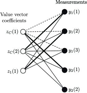
Figure 1: Graphical representation of the dependencies between value vector coefficients and compressive measurements for the signal ensemble $X$ and location matrix $P$ discussed in Example 3. Each edge in this graph denotes a dependency of a measurement on a value vector coefficient, but dashed lines indicate dependencies that cannot be exploited due to overlap of common and innovation coefficients. Among the edges that remain, the thick solid lines indicate the existence of a matching from each value vector coefficient to a distinct measurement; the existence of such a matching ensures that the system of equations $Y=\Phi P\Theta$ is invertible (see Theorem 1 and its proof in Section IV). Measurements that remain unassigned in this matching can then be used to verify the correctness of the solution (see Theorem 3 and its proof in Appendix B).

IV Central Proof and Bipartite Graph Formulation

This section is dedicated to proving Theorem 1. In order to prove this theorem, we introduce a bipartite graph formulation that represents the dependencies between the obtained measurements $Y$ and the coefficients in the value vector $\Theta$.

IV-A Proof of Theorem 1

For brevity, we denote $K_{C}(P)$ and $K_{j}(P)$ simply as $K_{C}$ and $K_{j}$. We denote the number of columns of $P$ by

$${D^{\prime}}={D^{\prime}}(P):=K_{C}+\sum_{j\in\Lambda}K_{j},$$ (22)

and note that $D^{\prime}\geq D$. Because $P\in\mathcal{P}_{F}(X)$, there exists $\Theta\in\mathbb{R}^{D^{\prime}}$ such that $X=P\Theta$. Because $Y=\Phi X$, $\Theta$ is a solution to $Y=\Phi P\Theta$.

We will argue that, with probability one over $\Phi$, $\Upsilon:=\Phi P$ has rank ${D^{\prime}}$, and thus $\Theta$ is the unique solution to the equation $Y=\Phi P\Theta=\Upsilon\Theta$. To prove that $\Upsilon$ has rank ${D^{\prime}}$, we invoke the following lemma, which we prove in Section IV-B.

Lemma 1

If (19) holds, then there exists a mapping $\mathcal{C}:\{1,2,\dots,K_{C}\}\rightarrow\Lambda$, assigning each element of the common component to one of the sensors, such that for all nonempty subsets $\Gamma\subseteq\Lambda$,

$$\sum_{j\in\Gamma}M_{j}\;\geq\;\sum_{j\in\Gamma}(K_{j}+C_{j}),$$ (23)

where $C_{j}:=|\{k\in\{1,2,\dots,K_{C}\}:~{}\mathcal{C}(k)=j\}|$ for each $j\in\Lambda$, and such that for each $k\in\{1,2,\dots,K_{C}\}$, the $k^{\mathrm{th}}$ column of $P_{C}$ is not a column of $P_{\mathcal{C}(k)}$.

Intuitively, the existence of such a mapping suggests that ($i$) each sensor has taken enough measurements to cover its own innovation component (requiring $K_{j}$ measurements) and perhaps some of the common component, ($ii$) for any $\Gamma\subseteq\Lambda$, the sensors in $\Gamma$ have collectively taken enough extra measurements to cover the requisite $K_{C}(\Gamma,P)$ elements of the common component, and ($iii$) the extra measurements are taken at sensors where the common and innovation components do not overlap. Formally, we will use the existence of such a mapping to prove that $\Upsilon$ has rank ${D^{\prime}}$.

We proceed by noting that $\Upsilon$ has the block structure illustrated in (5), where each $\Phi_{j}P_{C}$ (respectively, $\Phi_{j}P_{j}$) is an $M_{j}\times K_{C}$ (respectively, $M_{j}\times K_{j}$) submatrix of $\Phi_{j}$ obtained by selecting columns from $\Phi_{j}$ according to the columns contained in $P_{C}$ (respectively, $P_{j}$). Referring to (22), we see that, in total, $\Upsilon$ has ${D^{\prime}}$ columns. To argue that $\Upsilon$ has rank ${D^{\prime}}$, we will consider a sequence of three matrices $\Upsilon_{0}$, $\Upsilon_{1}$, and $\Upsilon_{2}$ constructed from modifications to $\Upsilon$.

Construction of $\Upsilon_{0}$: We begin by letting $\Upsilon_{0}$ denote the “partially zeroed” matrix obtained from $\Upsilon$ using the following construction:

1. Let $\Upsilon_{0}=\Upsilon$ and $k=1$.

2. For each $j$ such that $P_{j}$ has a column that matches column $k$ of $P_{C}$ (note that by Lemma 1 this cannot happen if $\mathcal{C}(k)=j$), let $k^{\prime}$ represent the column index of the full matrix $P$ where this column of $P_{j}$ occurs. Subtract column $k^{\prime}$ of $\Upsilon_{0}$ from column $k$ of $\Upsilon_{0}$. This forces to zero all entries of $\Upsilon_{0}$ formerly corresponding to column $k$ of the block $\Phi_{j}P_{C}$.

3. If $k<K_{C}$, then increment $k$ and go to step 2.

The matrix $\Upsilon_{0}$ is identical to $\Upsilon$ everywhere except on the first $K_{C}$ columns, where any portion of a column equal to a column of $\Phi_{j}P_{j}$ to its right has been set to zero. Thus, $\Upsilon_{0}$ satisfies the next two properties, which will be inherited by matrices $\Upsilon_{1}$ and $\Upsilon_{2}$ that we subsequently define:

1. Each entry of $\Upsilon_{0}$ is either zero or a Gaussian random variable.

2. All Gaussian random variables in $\Upsilon_{0}$ are i.i.d.

Finally, because $\Upsilon_{0}$ was constructed only by subtracting columns of $\Upsilon$ from one another, $\mathrm{rank}(\Upsilon_{0})=\mathrm{rank}(\Upsilon)$.

Construction of $\Upsilon_{1}$: We now let $\Upsilon_{1}$ be the matrix obtained from $\Upsilon_{0}$ using the following construction: For each $j\in\Lambda$, we select $K_{j}+C_{j}$ arbitrary rows from the portion of $\Upsilon_{0}$ corresponding to sensor $j$ (the first $M_{1}$ rows of $\Upsilon_{0}$ correspond to sensor $1$, the following $M_{2}$ rows correspond to sensor $2$, and so on). The resulting matrix $\Upsilon_{1}$ has

$$\sum_{j\in\Lambda}(K_{j}+C_{j})\;=\;\left(\sum_{j\in\Lambda}K_{j}\right)+K_{C}\;=\;{D^{\prime}}$$

rows; note that this is fewer than the number of rows in $\Upsilon_{0}$ if $K_{j}+C_{j}<M_{j}$ for any $j$. Also, because $\Upsilon_{1}$ was obtained by selecting a subset of rows from $\Upsilon_{0}$, it has ${D^{\prime}}$ columns (just like $\Upsilon_{0}$) and satisfies $\mathrm{rank}(\Upsilon_{1})\leq\mathrm{rank}(\Upsilon_{0})=\mathrm{rank}(\Upsilon)$.

Construction of $\Upsilon_{2}$: We now let $\Upsilon_{2}$ be the ${D^{\prime}}\times{D^{\prime}}$ matrix obtained by permuting columns of $\Upsilon_{1}$ using the following construction:

1. Let $\Upsilon_{2}=[~{}]$, and let $j=1$.

2. For each $k$ such that $\mathcal{C}(k)=j$, let $\Upsilon_{1}(k)$ denote the $k^{\mathrm{th}}$ column of $\Upsilon_{1}$, and concatenate $\Upsilon_{1}(k)$ to $\Upsilon_{2}$, i.e., let $\Upsilon_{2}\leftarrow[\Upsilon_{2}~{}\Upsilon_{1}(k)]$. There are $C_{j}$ such columns.

3. Let $\Upsilon_{1,j}$ denote the columns of $\Upsilon_{1}$ corresponding to the entries of $\Phi_{j}P_{j}$ (the innovation components of sensor $j$), and concatenate $\Upsilon_{1,j}$ to $\Upsilon_{2}$, i.e., let $\Upsilon_{2}\leftarrow[\Upsilon_{2}~{}\Upsilon_{1,j}]$. There are $K_{j}$ such columns.

4. If $j<J$, then increment $j$ and go to Step 2.

In total, Step 2 chooses $\sum_{j=1}^{J}C_{j}=K_{C}$ columns, while Step 3 chooses $\sum_{j=1}^{J}K_{j}$ columns, and thus referring to (22), $\Upsilon_{2}$ has $K_{C}+\sum_{j=1}^{J}K_{j}=D^{\prime}$ columns. The number of rows is the same as that of $\Upsilon_{1}$, making $\Upsilon_{2}$ a square matrix. Because $\Upsilon_{1}$ and $\Upsilon_{2}$ share the same columns up to reordering, it follows that

$$\mathrm{rank}(\Upsilon_{2})=\mathrm{rank}(\Upsilon_{1})\leq\mathrm{rank}(\Upsilon).$$ (24)

Based on its dependency on $\Upsilon_{0}$, and following from Lemma 1, $\Upsilon_{2}$ meets properties P1 and P2 defined above in addition to a third property:

1. All entries along the main diagonal of $\Upsilon_{2}$ are Gaussian random variables (none are deterministically zero).

Property P3 follows because each diagonal element of $\Upsilon_{2}$ will either be an entry of some $\Phi_{j}P_{j}$, which remains Gaussian throughout our constructions, or it will be an entry of some $k^{\mathrm{th}}$ column of some $\Phi_{j}P_{C}$ for which $\mathcal{C}(k)=j$. In the latter case, we know by Lemma 1 and the construction of $\Upsilon_{0}$ (Step 2) that the $k^{\mathrm{th}}$ column of $\Phi_{j}P_{C}$ is not zeroed out, and thus the corresponding diagonal entry remains Gaussian throughout our constructions.

Having identified these three properties satisfied by $\Upsilon_{2}$, we will prove by induction that, with probability one over $\Phi$, such a matrix has full rank.

Lemma 2

Let $\Upsilon^{(d-1)}$ be a $(d-1)\times(d-1)$ matrix having full rank. Construct a $d\times d$ matrix $\Upsilon^{(d)}$ as follows:

$$\Upsilon^{(d)}:=\left[\begin{array}[]{cc}\Upsilon^{(d-1)}&v_{1}\\ v_{2}^{T}&\omega\end{array}\right]$$

where $v_{1},v_{2}\in\mathbb{R}^{d-1}$ are column vectors with each entry being either zero or a Gaussian random variable, $\omega$ is a Gaussian random variable, and all random variables are i.i.d. and independent of $\Upsilon^{(d-1)}$. Then with probability one, $\Upsilon^{(d)}$ has full rank.

Applying Lemma 2 inductively ${D^{\prime}}$ times, the success probability remains one. It follows that with probability one over $\Phi$, $\mathrm{rank}(\Upsilon_{2})={D^{\prime}}$. Combining this last result with (24), we conclude that $\mathrm{rank}(\Upsilon)={D^{\prime}}$ with probability one over $\Phi$. It remains to prove Lemma 2.

Proof of Lemma 2: When $d=1$, $\Upsilon^{(d)}=[\omega]$, which has full rank if and only if $\omega\neq 0$, which occurs with probability one.

When $d>1$, using expansion by minors, the determinant of $\Upsilon^{(d)}$ satisfies $\det(\Upsilon^{(d)})=\omega\cdot\det(\Upsilon^{(d-1)})+C,$ where $C=C(\Upsilon^{(d-1)},v_{1},v_{2})$ is independent of $\omega$. The matrix $\Upsilon^{(d)}$ has full rank if and only if $\det(\Upsilon^{(d)})\neq 0$, which is satisfied if and only if $\omega\neq\frac{-C}{\det(\Upsilon^{(d-1)})}.$ By the inductive assumption, $\det(\Upsilon^{(d-1)})\neq 0$ and $\omega$ is a Gaussian random variable that is independent of $C$ and $\det(\Upsilon^{(d-1)})$. Thus, $\omega\neq\frac{-C}{\det(\Upsilon^{(d-1)})}$ with probability one. ∎

IV-B Proof of Lemma 1

To prove Lemma 1, we apply tools from graph theory.

We introduce a bipartite graph $G=(V_{V},V_{M},E)$ that captures the dependencies between the entries of the value vector $\Theta\in\mathbb{R}^{D^{\prime}}$ and the entries of the measurement vector $Y=\Phi P\Theta$. This graph is defined as follows. The set of value vertices $V_{V}$ has elements with indices $d\in\{1,\ldots,D^{\prime}\}$ representing the entries $\Theta(d)$ of the value vector. The set of measurement vertices $V_{M}$ has elements with indices $(j,m)$ representing the measurements $y_{j}(m)$, with $j\in\Lambda$ and $m\in\{1,\ldots,M_{j}\}$ (the range of possible $m$ varies depending on $j$). The cardinalities for these sets are $|V_{V}|=D^{\prime}$ and $|V_{M}|=\sum_{j\in\Lambda}M_{j}$. Finally, the set of edges $E$ is defined according to the following rules:

• For every $d\in\{1,2,\dots,K_{C}\}\subseteq V_{V}$ and $j\in\Lambda$ such that column $d$ of $P_{C}$ does not also appear as a column of $P_{j}$, we have an edge connecting $d$ to each vertex $(j,m)\in V_{M}$ for $1\leq m\leq M_{j}$.

• For every $d\in\{K_{C}+1,K_{C}+2,\dots,{D^{\prime}}\}\subseteq V_{V}$, we consider the sensor $j$ associated with column $d$ of $P$, and we have an edge connecting $d$ to each vertex $(j,m)\in V_{M}$ for $1\leq m\leq M_{j}$.

An example graph for a distributed sensing setting appears in Figure 2.

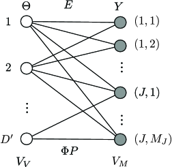
Figure 2: The bipartite graph $G=(V_{V},V_{M},E)$ indicates the relationship between the value vector coefficients and the measurements.

We seek a matching within the bipartite graph $G=(V_{V},V_{M},E)$, namely, a subgraph $(V_{V},V_{M},\overline{E})$ with $\overline{E}\subseteq E$ that pairs each element of $V_{V}$ with a unique element of $V_{M}$. Such a matching will immediately give us the desired mapping $\mathcal{C}$ as follows: for each $k\in\{1,2,\dots,K_{C}\}\subseteq V_{V}$, let $(j,m)\in V_{M}$ denote the single vertex matched to $k$ by an edge in $\overline{E}$; we then set $\mathcal{C}(k)=j$.

To prove the existence of such a matching within the graph, we invoke a version of Hall’s marriage theorem for bipartite graphs [24]. Hall’s theorem states that within a bipartite graph $(V_{1},V_{2},E)$, there exists a matching that assigns each element of $V_{1}$ to a unique element of $V_{2}$ if for any collection of elements $\Pi\subseteq V_{1}$, the set $E(\Pi)$ of neighbors of $\Pi$ in $V_{2}$ has cardinality $|E(\Pi)|\geq|\Pi|$. To apply Hall’s theorem in the context of our lemma, we will show that if (19) is satisfied, then for any set $\Pi\subseteq V_{V}$ of entries in the value vector, the set $E(\Pi)$ of neighbors of $\Pi$ in $V_{M}$ has size $|E(\Pi)|\geq|\Pi|$.

Let us consider an arbitrary set $\Pi\subseteq V_{V}$. We let $S_{\Pi}=\{j\in\Lambda:(j,m)\in E(\Pi)\mathrm{~{}for~{}some~{}}m\}\subseteq\Lambda$ denote the set of signal indices whose measurement vertices have edges that connect to $\Pi$. Since a connection between a value vertex and a measurement vertex at a given sensor implies a connection to all other measurement vertices for that sensor, it follows that $|E(\Pi)|=\sum_{j\in S_{\Pi}}M_{j}$. Thus, in order to satisfy Hall’s condition for $\Pi$, we require

$$\sum_{j\in S_{\Pi}}M_{j}\geq|\Pi|.$$ (25)

We would now like to show that $\sum_{j\in S_{\Pi}}K_{j}+K_{C}(S_{\Pi},P)\geq|\Pi|$, and thus if (19) is satisfied for all $\Gamma\subseteq\Lambda$, then (25) is satisfied in particular for $S_{\Pi}\subseteq\Lambda$.

In general, the set $\Pi$ may contain vertices for both common components and innovation components. We write $\Pi=\Pi_{C}\cup\Pi_{I}$ to denote the disjoint union of these two sets.

By construction, $|\Pi_{I}|\leq\sum_{j\in S_{\Pi}}K_{j}$, because $\Pi_{I}$ cannot include any innovation component outside the set of sensors $S_{\Pi}$. We will also argue that $|\Pi_{C}|\leq K_{C}(S_{\Pi},P)$ as follows. By definition, for a set $\Gamma\subseteq\Lambda$, $K_{C}(\Gamma,P)$ counts the number of columns in $P_{C}$ that also appear in $P_{j}$ for all $j\notin\Gamma$. By construction, for each $k\in\Pi_{C}$, vertex $k$ has no connection to vertices $(j,m)$ for $j\notin S_{\Pi}$, and so it must follow that the $k^{\mathrm{th}}$ column of $P_{C}$ is present in $P_{j}$ for all $j\notin S_{\Pi}$. Thus, the index $k$ is among the indices counted in the definition (18) of $K_{C}(S_{\Pi},P)$, and therefore $|\Pi_{C}|\leq K_{C}(S_{\Pi},P)$.

We conclude that $|\Pi|=|\Pi_{I}|+|\Pi_{C}|\leq\sum_{j\in S_{\Pi}}K_{j}+K_{C}(S_{\Pi},P)$, and so (19) implies (25) for any $\Pi$, and so Hall’s condition is satisfied, and a matching exists. Finally, consider any set $\Gamma\subseteq\Lambda$. To confirm that (23) holds for this set, note that there are a total of $\sum_{j\in\Gamma}M_{j}$ vertices $(j,m)\in V_{M}$ such that $j\in\Gamma$. Each of these vertices is matched to at most one vertex in $V_{V}$, which must correspond either to an innovation component counted in $K_{j}$ for some $j\in\Gamma$ or to a common component indexed by some $k$ such that $\mathcal{C}(k)\in\Gamma$. It follows that $\sum_{j\in\Gamma}M_{j}\geq\sum_{j\in\Gamma}(K_{j}+C_{j})$. ∎

V Discussion

In this paper, we have introduced the ensemble sparsity model (ESM) framework for modeling intra- and inter-signal dependencies within a collection of sparse signals. This framework is based on a factored representation of the signal ensemble that decouples its location information from its value information. We have also proposed an analytical framework based on bipartite graphs that allowed us, in the context of a common/innovation ESM $\mathcal{P}$, to characterize the numbers of measurements $M_{1},M_{2},\dots,M_{J}$ needed for successful recovery of a signal ensemble $X$. Our bounds highlight the benefit of joint reconstruction in distributed compressive sensing (DCS), since sparse signals can be recovered from fewer measurements than their nominal sparsity level would indicate.

The factored representation that we have proposed for modeling sparse signal ensembles is closely related to the recently proposed union-of-subspaces modeling frameworks for CS [25, 26, 27, 28]. What is particularly novel about our treatment is the explicit consideration of the block structure of matrices such as $P$ and $\Phi$, and the explicit accounting for measurement bounds on a sensor-by-sensor basis. Most of the conventional union-of-subspaces theory in CS is intended to characterize the number of measurements required to recover a vector $X$ from measurements $\Phi X$, where $\Phi$ is a dense matrix.

Finally, as we have discussed in Section II-E, common/innovation ESMs can be populated using various choices of matrices $P$ of the form (1). Our bounds in Section III are relatively agnostic to such design choices. Past experience, however, has indicated that practical algorithms for signal recovery can benefit from being tuned to the particular type of signal dependencies under consideration [5, 12, 13, 14, 15, 19, 20, 29, 30, 21, 31, 32, 33, 18]. Our focus in this paper has been not on tractable recovery algorithms or robustness issues, but rather on foundational limits governing how the measurements may be amortized across the sensors while preserving the information required to uniquely identify the sparse signal ensemble. However, we believe that our results and our graphical modeling framework may pave the way for a better, perhaps more unified, development of practical DCS algorithms.

Appendix A Proof of Theorem 2

As in (22), we let ${D^{\prime}}$ denote the number of columns in $P$. Because $P\in\mathcal{P}_{F}(X)$, there exists $\Theta\in\mathbb{R}^{D^{\prime}}$ such that $X=P\Theta$. Because $Y=\Phi X$, then $\Theta$ is a solution to $Y=\Phi P\Theta$. We will argue for $\Upsilon:=\Phi P$ that $\mathrm{rank}(\Upsilon)<{D^{\prime}}$, and thus there exists $\widehat{\Theta}\neq\Theta$ such that $Y=\Upsilon\Theta=\Upsilon\widehat{\Theta}$. Since $P$ has full rank, it follows that $\widehat{X}:=P\widehat{\Theta}\neq P\Theta=X$.

We let $\Upsilon_{0}$ be the “partially zeroed” matrix obtained from $\Upsilon$ using the identical procedure detailed in Section IV-A. Again, because $\Upsilon_{0}$ was constructed only by subtracting columns of $\Upsilon$ from one another, it follows that $\mathrm{rank}(\Upsilon_{0})=\mathrm{rank}(\Upsilon)$.

Suppose that $\Gamma\subseteq\Lambda$ is a set for which (20) holds. We let $\Upsilon_{3}$ be the submatrix of $\Upsilon_{0}$ obtained by selecting the following columns:

• For any $k\in\{1,2,\dots,K_{C}\}$ such that column $k$ of $P_{C}$ also appears as a column in $P_{j}$ for all $j\notin\Gamma$, we include column $k$ of $\Upsilon_{0}$ as a column in $\Upsilon_{3}$. There are $K_{C}(\Gamma,P)$ such columns $k$.

• For any $k\in\{K_{C}+1,K_{C}+2,\dots,{D^{\prime}}\}$ such that column $k$ of $P$ corresponds to an innovation for some sensor $j\in\Gamma$, we include column $k$ of $\Upsilon_{0}$ as a column in $\Upsilon_{3}$. There are $\sum_{j\in\Gamma}K_{j}$ such columns $k$.

This submatrix has $\sum_{j\in\Gamma}K_{j}+K_{C}(\Gamma,P)$ columns. Because $\Upsilon_{0}$ has the same size as $\Upsilon$ (see Section IV-A), and in particular has only ${D^{\prime}}$ columns, then in order to have that $\mathrm{rank}(\Upsilon_{0})={D^{\prime}}$, it is necessary that all $\sum_{j\in\Gamma}K_{j}+K_{C}(\Gamma,P)$ columns of $\Upsilon_{3}$ be linearly independent.

Based on the method described for constructing $\Upsilon_{0}$, it follows that $\Upsilon_{3}$ is zero for all measurement rows not corresponding to the set $\Gamma$. These rows were nonzero only for two sets of columns of $\Upsilon_{0}$: ($i$) the columns corresponding to the innovations for signals $j\notin\Gamma$, and ($ii$) the columns $k\in\{1,2,\ldots,K_{C}\}$ for which the $k^{th}$ column of $P_{C}$ appears in none of the matrices $P_{j},j\notin\Gamma$. Both of these sets of columns are discarded during the construction of $\Upsilon_{3}$. Therefore, consider the submatrix $\Upsilon_{4}$ of $\Upsilon_{3}$ obtained by selecting only the measurement rows corresponding to the set $\Gamma$. Because all the rows discarded from $\Upsilon_{3}$ are zero, it follows that $\mathrm{rank}(\Upsilon_{3})=\mathrm{rank}(\Upsilon_{4})$. However, since $\Upsilon_{4}$ has only $\sum_{j\in\Gamma}M_{j}$ rows, we invoke (20) and have that $\mathrm{rank}(\Upsilon_{3})=\mathrm{rank}(\Upsilon_{4})\leq\sum_{j\in\Gamma}M_{j}<\sum_{j\in\Gamma}K_{j}+K_{C}(\Gamma,P)$. Thus, all $\sum_{j\in\Gamma}K_{j}+K_{C}(\Gamma,P)$ columns of $\Upsilon_{3}$ cannot be linearly independent, and so $\Upsilon$ does not have full rank. This means that there exists $\widehat{\Theta}\neq\Theta$ such that $Y=\Upsilon\Theta=\Upsilon\widehat{\Theta}$, and thus we cannot distinguish between the two solutions $\widehat{X}:=P\widehat{\Theta}\neq P\Theta=X$. ∎

Appendix B Proof of Theorem 3

Given the measurements $Y$ and measurement matrix $\Phi$, we will show that it is possible to recover some $P\in\mathcal{P}_{F}(X)$ and a corresponding vector $\Theta$ such that $X=P\Theta$ using the following algorithm.

• Extract from each measurement vector $y_{j}$ its final entry, and sum these entries to obtain the quantity $\overline{y}=\sum_{j\in\Gamma}y_{j}(M_{j})$. Similarly, add the corresponding rows of $\Phi$ into a single row $\overline{\phi}^{T}$. The row vector $\overline{\phi}^{T}$ is a concatenation of the final rows of the matrices $\Phi_{j}$, and thus its entries are i.i.d. Gaussian. Note that $\overline{y}=\overline{\phi}^{T}X$; this quantity will be used in a cross-validation step below.

• Group the remaining $\left(\sum_{j\in\Lambda}M_{j}\right)-J$ measurements into a vector $\overline{Y}$, and let $\overline{\Phi}$ contain the corresponding rows of $\Phi$. We note that $\overline{\phi}$ is independent from $\overline{\Phi}$ and that $\overline{Y}=\overline{\Phi}X$.

• For each matrix $P\in\mathcal{P}$ such that $\overline{Y}\in\mathrm{colspan}(\overline{\Phi}P)$, choose a single solution $\Theta_{P}$ to $\overline{Y}=\overline{\Phi}P\Theta_{P}$ independently of $\overline{\phi}$. Then, perform the following cross-validation: if $\overline{y}=\overline{\phi}^{T}P\Theta_{P}$, then return the estimate $\widehat{X}=P\Theta_{P}$; otherwise, continue with the next matrix $P$.

We begin by noting that there exists at least one matrix $P\in\mathcal{P}$ for which $\overline{Y}\in\mathrm{colspan}(\overline{\Phi}P)$ and for which $X=P\Theta_{P}$. In particular, consider the matrix $P^{*}\in\mathcal{P}_{F}(X)$ mentioned in the theorem statement. Because (21) holds for $P^{*}$, Theorem 1 guarantees that with probability one, $\overline{\Phi}P^{*}$ will have full rank, and so there is a unique solution $\Theta_{P^{*}}$ to $\overline{Y}=\overline{\Phi}P^{*}\Theta_{P^{*}}$. Since $P^{*}\in\mathcal{P}_{F}(X)$ and $P^{*}$ is full rank, we know that $X=P^{*}\Theta_{P^{*}}$. Also, since $Y=\Phi X$, we know that $\overline{y}=\overline{\phi}^{T}P^{*}\Theta_{P^{*}}$, and so this matrix will clear the cross-validation step.

Now suppose that, for some $P\in\mathcal{P}$, the algorithm above considers a candidate solution $\Theta_{P}$ to $\overline{Y}=\overline{\Phi}P\Theta_{P}$, but suppose also that $X\neq P\Theta_{P}$. The algorithm will fail to discard this incorrect solution if $\Theta_{P}$ passes the cross-validation test, i.e., if $\overline{\phi}^{T}P\Theta_{P}=\overline{y}=\overline{\phi}^{T}X$. Recall, however, that $\overline{\phi}$ is an i.i.d. Gaussian random vector and that it is independent of both $X$ and $P\Theta_{P}$. It then follows that $\overline{\phi}$ is orthogonal to $X-P\Theta_{P}$ with probability zero, and therefore we will have $\overline{\phi}^{T}(X-P\Theta_{P})\neq 0$ (equivalently, $\overline{\phi}^{T}P\Theta_{P}\neq\overline{y}$) with probability one. Therefore, this incorrect solution will be discarded with probability one. Since $\mathcal{P}$ contains only a finite number of matrices, the probability of cross-validation discarding all incorrect solutions remains one. ∎

Marco F. Duarte (S’99–M’09) received the B.Sc. degree in computer engineering (with distinction) and the M.Sc. degree in electrical engineering from the University of Wisconsin-Madison in 2002 and 2004, respectively, and the Ph.D. degree in electrical engineering from Rice University, Houston, TX, in 2009. He was an NSF/IPAM Mathematical Sciences Postdoctoral Research Fellow in the Program of Applied and Computational Mathematics at Princeton University, Princeton, NJ, from 2009 to 2010, and in the Department of Computer Science at Duke University, Durham, NC, from 2010 to 2011. He is currently an Assistant Professor in the Department of Electrical and Computer Engineering at the University of Massachusetts, Amherst, MA. His research interests include machine learning, compressed sensing, sensor networks, and optical image coding. Dr. Duarte received the Presidential Fellowship and the Texas Instruments Distinguished Fellowship in 2004 and the Hershel M. Rich Invention Award in 2007, all from Rice University. He is also a member of Tau Beta Pi.

Michael B. Wakin (S’01–M’07) received the B.A. degree in mathematics in 2000, and the B.Sc., M.Sc., and Ph.D. degrees, all in electrical engineering, all from Rice University, Houston, TX, in 2000, 2002, and 2007, respectively. He was an NSF Mathematical Sciences Postdoctoral Research Fellow with the California Institute of Technology, Pasadena, from 2006 to 2007, and an Assistant Professor with the University of Michigan, Ann Arbor, from 2007 to 2008. He is currently an Assistant Professor with the Department of Electrical Engineering and Computer Science at the Colorado School of Mines. His research interests include sparse, geometric, and manifold-based models for signal and image processing, approximation, compression, compressive sensing, and dimensionality reduction Dr. Wakin shared the Hershel M. Rich Invention Award in 2007 from Rice University for the design of a single-pixel camera based on compressive sensing; in 2008, he received the DARPA Young Faculty Award for his research in compressive multisignal processing; and in 2012, he received the NSF CAREER Award for research into dimensionality reduction techniques for structured data sets.

Dror Baron (M’03–SM’10) received the B.Sc. (summa cum laude) and M.Sc. degrees from the Technion—Israel Institute of Technology, Haifa, in 1997 and 1999, and the Ph.D. degree from the University of Illinois at Urbana-Champaign in 2003, all in electrical engineering. From 1997 to 1999, he was with Witcom Ltd., working in modem design. From 1999 to 2003, he was a Research Assistant at the University of Illinois at Urbana-Champaign, where he was also a Visiting Assistant Professor in 2003. He was a Postdoctoral Research Associate in the Department of Electrical and Computer Engineering at Rice University, Houston, TX, from 2003 to 2006. He was a quantitative financial analyst with Menta Capital, San Francisco, CA, from 2007 to 2008, and a Visiting Scientist in the Department of Electrical Engineering at the Technion—Israel Institute of Technology, Haifa, from 2008 to 2010. He is currently an Assistant Professor in the Electrical and Computer Engineering Department at the North Carolina State University. His research interests combine information theory, signal processing, and fast algorithms; in recent years, he has focused on compressed sensing. Dr. Baron was a recipient of the 2002 M. E. Van Valkenburg Graduate Research Award, and received honorable mention at the Robert Bohrer Memorial Student Workshop in April 2002, both at the University of Illinois. He also participated from 1994 to 1997 in the Program for Outstanding Students, comprising the top 0.5% of undergraduates at the Technion.

Shriram Sarvotham (S’00–M’01) received the B.Tech. degree from the Indian Institute of Technology, Madras, India, and the M.S. and Ph.D. degrees from Rice University, Houston, TX, all in electrical engineering. His research interests lie in the broad areas of compressed sensing, nonasymptotic information theory, and Internet traffic analysis and modeling. Currently, he works as a Principal Research Scientist at Halliburton Energy Services, Houston, TX, where he investigates optimal data acquisition and processing of NMR data in oil and gas exploration.

Richard G. Baraniuk (M’93–SM’98–F’01) received the B.Sc. degree in 1987 from the University of Manitoba (Canada), the M.Sc. degree in 1988 from the University of Wisconsin-Madison, and the Ph.D. degree in 1992 from the University of Illinois at Urbana-Champaign, all in Electrical Engineering. After spending 1992–1993 with the Signal Processing Laboratory of Ecole Normale Supérieure, in Lyon, France, he joined Rice University, where he is currently the Victor E. Cameron Professor of Electrical and Computer Engineering. His research interests lie in the areas of signal processing, machine learning, and open education. Dr. Baraniuk received a NATO postdoctoral fellowship from NSERC in 1992, the National Young Investigator award from the National Science Foundation in 1994, a Young Investigator Award from the Office of Naval Research in 1995, the Rosenbaum Fellowship from the Isaac Newton Institute of Cambridge University in 1998, the C. Holmes MacDonald National Outstanding Teaching Award from Eta Kappa Nu in 1999, the University of Illinois ECE Young Alumni Achievement Award in 2000, the Tech Museum Laureate Award from the Tech Museum of Innovation in 2006, the Wavelet Pioneer Award from SPIE in 2008, the Internet Pioneer Award from the Berkman Center for Internet and Society at Harvard Law School in 2008, the World Technology Network Education Award and IEEE Signal Processing Society Magazine Column Award in 2009, the IEEE-SPS Education Award in 2010, the WISE Education Award in 2011, and the SPIE Compressive Sampling Pioneer Award in 2012. In 2007, he was selected as one of Edutopia Magazine’s Daring Dozen educators, and the Rice single-pixel compressive camera was selected by MIT Technology Review Magazine as a TR10 Top 10 Emerging Technology. He was elected a Fellow of the IEEE in 2001 and of AAAS in 2009.

References

- [1] M. F. Duarte, S. Sarvotham, D. Baron, M. B. Wakin, and R. G. Baraniuk, “Performance limits for jointly sparse signals via graphical models,” in Workshop Sensor, Signal, Inf. Proc. (SENSIP), (Sedona, AZ), May 2008.
- [2] M. F. Duarte, S. Sarvotham, M. B. Wakin, D. Baron, and R. G. Baraniuk, “Theoretical performance limits for jointly sparse signals via graphical models,” Tech. Rep. TREE0809, Rice University, Houston, TX, July 2008.
- [3] E. Candès, J. Romberg, and T. Tao, “Robust uncertainty principles: Exact signal reconstruction from highly incomplete frequency information,” IEEE Trans. Inf. Theory, vol. 52, pp. 489–509, Feb. 2006.
- [4] D. Donoho, “Compressed sensing,” IEEE Trans. Inf. Theory, vol. 52, pp. 1289–1306, Apr. 2006.
- [5] D. Baron, M. F. Duarte, S. Sarvotham, M. B. Wakin, and R. G. Baraniuk, “Distributed compressed sensing,” Tech. Rep. TREE0612, Rice University, Houston, TX, Nov. 2006.
- [6] J. Tropp and A. C. Gilbert, “Signal recovery from partial information via orthogonal matching pursuit,” IEEE Trans. Inf. Theory, vol. 53, pp. 4655–4666, Dec. 2007.
- [7] D. Needell and J. A. Tropp, “CoSaMP: Iterative signal recovery from incomplete and inaccurate samples,” Applied and Computational Harmonic Analysis, vol. 26, no. 3, pp. 301–321, 2009.
- [8] W. U. Bajwa, J. D. Haupt, A. M. Sayeed, and R. D. Nowak, “Joint source-channel communication for distributed estimation in sensor networks,” IEEE Trans. Inf. Theory, vol. 53, pp. 3629–3653, Oct. 2007.
- [9] M. Rabbat, J. D. Haupt, A. Singh, and R. D. Nowak, “Decentralized compression and predistribution via randomized gossiping,” in Int. Workshop Inf. Proc. Sensor Networks (IPSN), (Nashville, TN), pp. 51–59, Apr. 2006.
- [10] W. Wang, M. Garofalakis, and K. Ramchandran, “Distributed sparse random projections for refinable approximation,” in Int. Workshop Inf. Proc. Sensor Networks (IPSN), (Cambridge, MA), pp. 331–339, Apr. 2007.
- [11] S. Aeron, M. Zhao, and V. Saligrama, “On sensing capacity of sensor networks for the class of linear observation, fixed SNR models,” in IEEE Workshop Stat. Signal Proc. (SSP), (Madison, WI), pp. 388–392, Aug. 2007.
- [12] D. Baron, M. F. Duarte, S. Sarvotham, M. B. Wakin, and R. G. Baraniuk, “An information-theoretic approach to distributed compressed sensing,” in Allerton Conf. Comm., Control, Comput., (Monticello, IL), pp. 814–825, Sept. 2005.
- [13] M. F. Duarte, S. Sarvotham, D. Baron, M. B. Wakin, and R. G. Baraniuk, “Distributed compressed sensing of jointly sparse signals,” in Asilomar Conf. Signals, Systems and Computers, (Pacific Grove, CA), pp. 1537–1541, Nov. 2005.
- [14] M. B. Wakin, S. Sarvotham, M. F. Duarte, D. Baron, and R. G. Baraniuk, “Recovery of jointly sparse signals from few random projections,” in Proc. Neural Inf. Proc. Sys. (NIPS), (Vancouver, Canada), pp. 1435–1442, Nov. 2005.
- [15] M. F. Duarte, M. B. Wakin, D. Baron, and R. G. Baraniuk, “Universal distributed sensing via random projections,” in Int. Workshop Inf. Proc. Sensor Networks (IPSN), (Nashville, TN), pp. 177–185, Apr. 2006.
- [16] D. Slepian and J. K. Wolf, “Noiseless coding of correlated information sources,” IEEE Trans. Inf. Theory, vol. 19, pp. 471–480, July 1973.
- [17] T. M. Cover and J. A. Thomas, Elements of Information Theory. New York: Wiley, 1991.
- [18] A. Jalali, P. Ravikumar, S. Sanghavi, and C. Ruan, “A dirty model for multi-task learning,” in Proc. Neural Inf. Proc. Sys. (NIPS), vol. 23, 2010.
- [19] M. Fornassier and H. Rauhut, “Recovery algorithms for vector valued data with joint sparsity constraints,” SIAM Journal on Numerical Analysis, vol. 46, no. 2, pp. 577–613, 2008.
- [20] M. Mishali and Y. Eldar, “Reduce and boost: Recovering arbitrary sets of jointly sparse vectors,” IEEE Trans. Signal Proc., vol. 56, pp. 4692–4702, Oct. 2008.
- [21] S. R. Schnelle, J. N. Laska, C. Hegde, M. F. Duarte, M. Davenport, and R. G. Baraniuk, “Texas Hold’Em algorithms for distributed compressive sensing,” in IEEE Int. Conf. Acoustics, Speech, Signal Proc. (ICASSP), (Dallas, TX), pp. 2886–2889, Mar. 2010.
- [22] C. Berge, The Theory of Graphs. Mineola, NY: Dover, 2001.
- [23] R. Venkataramani and Y. Bresler, “Further results on spectrum blind sampling of 2D signals,” in IEEE Int. Conf. Image Proc. (ICIP), vol. 2, (Chicago), pp. 752–756, Oct. 1998.
- [24] D. B. West, Introduction to Graph Theory. Prentice Hall, 1996.
- [25] Y. M. Lu and M. N. Do, “Sampling signals from a union of subspaces,” IEEE Signal Processing Mag., vol. 25, pp. 41–47, Mar. 2008.
- [26] T. Blumensath and M. E. Davies, “Sampling theorems for signals from the union of finite-dimensional linear subspaces,” IEEE Trans. Inf. Theory, vol. 55, pp. 1872–1882, Apr. 2009.
- [27] Y. Eldar and M. Mishali, “Robust recovery of signals from a structured union of subspaces,” IEEE Trans. Inf. Theory, vol. 55, pp. 5302–5316, Nov. 2009.
- [28] R. G. Baraniuk, V. Cevher, M. F. Duarte, and C. Hegde, “Model-based compressive sensing,” IEEE Trans. Inf. Theory, vol. 56, pp. 1982–2001, Apr. 2010.
- [29] Y. Eldar and H. Rauhut, “Average case analysis of multichannel sparse recovery using convex relaxation,” IEEE Trans. Inf. Theory, vol. 56, pp. 505–519, Jan. 2010.
- [30] E. van den Berg and M. P. Friedlander, “Theoretical and empirical results for recovery from multiple measurements,” IEEE Trans. Inf. Theory, vol. 56, pp. 2516–2527, May 2010.
- [31] K. Lee, Y. Bresler, and M. Junge, “Subspace methods for joint sparse recovery,” IEEE Trans. Inf. Theory, vol. 58, pp. 3613–3641, June 2012.
- [32] J. M. Kim, O. K. Lee, and J. C. Ye, “Compressive MUSIC: Revisiting the link between compressive sensing and array signal processing,” IEEE Trans. Inf. Theory, vol. 58, pp. 278–301, Jan. 2012.
- [33] M. Davies and Y. Eldar, “Rank awareness in joint sparse recovery,” IEEE Trans. Inf. Theory, vol. 58, pp. 1135–1146, Feb. 2012.