Repetitive Reduction Patterns
in Lambda Calculus with letrec
(Work in Progress)

Abstract

For the λ-calculus with letrec we develop an optimisation, which is based on the contraction of a certain class of `future' (also: virtual) redexes.

In the implementation of functional programming languages it is common practice to perform β-reductions at compile time whenever possible in order to produce code that requires fewer reductions at run-time. This is, however, in principle limited to redexes and created redexes that are `visible' (in the sense that they can be contracted without the need for unsharing), and cannot generally be extended to redexes that are concealed by sharing constructs such as letrec. In the case of recursion, concealed redexes become visible only after unwindings during evaluation, and then have to be contracted time and again.

We observe that in some cases such redexes exhibit a certain form of repetitive behaviour at run time. We describe an analysis for identifying binders that give rise to such repetitive reduction patterns, and eliminate them by a sort of predictive contraction. Thereby these binders are lifted out of recursive positions or eliminated altogether, as a result alleviating the amount of β-reductions required for each recursive iteration.

Both our analysis and simplification are suitable to be integrated into existing compilers for functional programming languages as an additional optimisation phase. With this work we hope to contribute to increasing the efficiency of executing programs written in such languages.

In this extended abstract we report on work in progress carried out within the framework of the NWO project Realising Optimal Sharing. Instead of discussing optimal reduction in the λ-calculus, however, here we are concerned with a static analysis of $\lambda_{\textit{letrec}}$-terms which aims at removing $\beta$-redexes that are concealed by recursion constructs and cause cyclic migration of arguments during evaluation. We have to stress that our research on this particular topic is still in an early phase.

1 Introduction

In this work we study terms in $\lambda_{\textit{letrec}}$, i.e. in $\lambda$-calculus with an explicit letrec-construct for recursive definitions, that exhibit a form of repetitive reduction pattern when evaluated. We try to identify a class of such terms for which this behaviour can be avoided by a transformation into a term with, in some sense, the same semantic denotation. Even though the presented optimisation can be described directly for $\lambda_{\textit{letrec}}$-terms, and hence is applicable in all functional languages of which $\lambda_{\textit{letrec}}$ is a meaningful abstraction, we will use Haskell to denote examples of such terms and their optimised equivalents. Additionally, we depict terms as λ-graphs with explicit sharing-nodes (multiplexers) as used, for example, in [3].

A function well-known to Haskell programmers is the $\mathit{repeat}$ function that generates an infinite, constant stream of the supplied argument. A definition is easily found, namely:

An experienced Haskell programmer, however, would spot a `space leak', which refers to an $O(n)$ memory consumption for generating $n$ stream elements while $O(1)$ is possible, due to lazy evaluation. Therefore in the Haskell standard libraries that function is defined as:

The exact reasons for this difference in efficiency involve the characteristics of the deployed Haskell compiler and run-time system. A more direct and theoretical explanation can be attempted within the formal framework of $\lambda_{\textit{letrec}}$: The improved variant of $\mathit{repeat}$ does not require any β-reductions to produce further stream elements. That becomes apparent by the λ-graphs and their infinite unfoldings (Fig. 1). We use a rewriting relation arrow indexed by a triangle ($\mathrel{\rightarrow_{\medtriangledown}}$) to mark unfolding, regardless of whether sharing is expressed by a multiplexer or a letrec-binding.

 $\mathrel{{\twoheadrightarrow\twoheadrightarrow}_{\medtriangledown}}$         ${\twoheadrightarrow\twoheadrightarrow}_{β}$         $\mathrel{{\twoheadleftarrow\twoheadleftarrow}_{\medtriangledown}}$ 

Figure 1: Term graph representation of the two $\mathit{repeat}$ implementations and their unfoldings

From a software engineering perspective it is unsatisfactory that the programmer has to recognise and mitigate such cases. One might even consider the unoptimised version superior with respect to code clarity. Therefore we propose an analysis and transformation method to automate the optimisation, which then can be integrated into the compiler pipeline of existing functional language implementations. In the following sections we will work with simple examples to develop this method and successively generalise it for wider applicability.

2 Preliminaries

The method we describe applies to the $\lambda_{\textit{letrec}}$-calculus, which is a higher-order rewrite system. Still, in this work-in-progress report we primarily intend to motivate our research and outline the approaches developed so far. Hence, for the moment we give a largely informal description, and resort to first-order formulations, λ-graphs, or Haskell, whichever seems more suited.

Definition 1 (First-order representation of $\lambda_{\textit{letrec}}$)

Let $V$ be a set of variables. Then a $\lambda_{\textit{letrec}}$-term is defined as follows:

$$\begin{array}[]{lllll}(\textit{term})&T&::=&\lambda V.T&(\textit{abstraction})\\ &&|&T~{}T&(\textit{application})\\ &&|&V&(\textit{variable})\\ &&|&\texttt{letrec}~{}\mathit{Defs}~{}\texttt{in}~{}T&(\textit{letrec})\\ (\textit{definitions})&\mathit{Defs}&::=&v_{1}=T~{}\dots~{}v_{n}=T&(\textit{equations})\\ &&&v_{1},\dots,v_{n}\in V~{}\text{all distinct}\end{array}$$

But ultimately only a higher-order formulation can be formally satisfactory, thus we propose the following representation as a higher-order rewrite system (HRS) [14] for $\lambda_{\textit{letrec}}$.

Definition 2 (Higher-order representation of $\lambda_{\textit{letrec}}$)

Let $\mathit{Var}$ be a set of variables, and $\mathit{BTypes}$ a set of base types that induce the set $\mathit{Types}$ of simple types. The terms of $\lambda_{\textit{letrec}}$ are simply-typed higher-order terms over the HRS-signature that for all $n\in\mathbb{N}$, and all types $\tau_{0},\tau_{1},\ldots,\tau_{n}\in\mathit{Types}$ contains a symbol $\texttt{let}_{n}\texttt{\_in}$ of type:

$$\texttt{let}_{n}\texttt{\_in}\,:\,(\tau_{1}\times\ldots\times\tau_{n}\to\tau_{0}\times\tau_{1}\ldots\times\tau_{n})\to\tau_{0}$$

Product types are only used for better readability. We will use the symbols $t$, $s$, $u$ for terms in $\lambda_{\textit{letrec}}$.

Based on this notion of terms, the $\lambda_{\textit{letrec}}$-calculus consists of the rewrite relations: $\beta$-reduction, $\eta$-reduction, and letrec-unfolding. Additionally, we use the concept of generalised $\beta$-reduction [12].

For example, letrec-unfolding on the informal $\lambda_{\textit{letrec}}$-terms according to the grammar above could be described by the following rewrite rules:

$$\texttt{let}{\hskip 2.0pt}{f_{1}={s_{1}}({\vec{f}}),\ldots,f_{n}={s_{n}}({\vec{f}})}{\hskip 3.0pt\texttt{in}\hskip 5.0pt}{t}\,\,\,\rightarrow_{\medtriangledown}\,\,\,t\qquad\text{(if $f_{1},\ldots,f_{n}$ not free in $t$)}$$

$$\begin{aligned} &\texttt{let}{\hskip 2.0pt}{\underbrace{f_{1}={s_{1}}({\vec{f}}),\ldots,f_{n}={s_{n}}({\vec{f}})}_{\mathit{Defs}}}{\hskip 3.0pt\texttt{in}\hskip 5.0pt}{{t}({\vec{f}})}\,\,\,\rightarrow_{\medtriangledown}\,\,\,t\bigl{(}\texttt{let}{\hskip 2.0pt}{\mathit{Defs}}{\hskip 3.0pt\texttt{in}\hskip 5.0pt}{{s_{1}}({\vec{f}})},\ldots,\texttt{let}{\hskip 2.0pt}{\mathit{Defs}}{\hskip 3.0pt\texttt{in}\hskip 5.0pt}{{s_{n}}({\vec{f}})}\bigl{)}\end{aligned}$$

which, if translated into HRS-rules (using the signature defined in Def. 2), can take the following form:

$$\texttt{let}_{n}\texttt{\_in}{\hskip 2.0pt}{{{\lambda}{f_{1}\ldots f_{n}}}.\hskip 0.5pt{(Y,{Z_{1}}({\vec{f}}),\ldots,{Z_{n}}({\vec{f}}))}}\,\,\,\rightarrow_{\medtriangledown}\,\,\,Y$$

$$\begin{aligned} &\texttt{let}_{n}\texttt{\_in}{\hskip 2.0pt}{{{\lambda}{f_{1}\ldots f_{n}}}.\hskip 0.5pt{({Y}({\vec{f}}),{Z_{1}}({\vec{f}}),\ldots,{Z_{n}}({\vec{f}}))}}\,\,\,\rightarrow_{\medtriangledown}\,\,\,\\ &\hskip 103.33301ptY(\texttt{let}_{n}\texttt{\_in}{\hskip 2.0pt}{{{\lambda}{f_{1}\ldots f_{n}}}.\hskip 0.5pt{({{Z_{1}}({\vec{f}})},{Z_{1}}({\vec{f}}),\ldots,{Z_{n}}({\vec{f}}))}})\ldots\\ &\hskip 154.99951pt\phantom{Y}\ldots(\texttt{let}_{n}\texttt{\_in}{\hskip 2.0pt}{{{\lambda}{f_{1}\ldots f_{n}}}.\hskip 0.5pt{({{Z_{n}}({\vec{f}})},{Z_{1}}({\vec{f}}),\ldots,{Z_{n}}({\vec{f}}))}})\end{aligned}$$

Notation 3 (Rewrite relations in $\lambda_{\textit{letrec}}$)

On $\lambda_{\textit{letrec}}$-terms we consider the following rewrite relations: $\beta$-reduction denoted by $\rightarrow_{\beta}\,$; generalised $\beta$-reduction denoted by $\rightarrow_{g\beta}\,$; $\eta$-reduction denoted by $\rightarrow_{\eta}\,$; letrec-unfolding denoted by $\rightarrow_{\medtriangledown}$.

For each of these rewrite relations $\rightarrow$, the many-step rewrite relation with respect to $\rightarrow$ will be written as $\twoheadrightarrow$, and the (strongly convergent) infinite rewrite relation as ${\twoheadrightarrow\twoheadrightarrow}$.

With the transformation from Section 1, which is further developed in the next sections, we aim to convert a given term $t$ with repetitive reduction patterns into a term $t^{\prime}$ that does not require these reductions to be performed any more, but such that $t$ and $t^{\prime}$ are `operationally equivalent', in a sense that guarantees that important properties observable during evaluation are preserved.

One candidate for a precisely defined notion of operational equivalence is the extension to $\lambda_{\textit{letrec}}$-terms of `applicative bisimulation' on $\lambda$-terms due to Abramsky [2]. Two $\lambda_{\textit{letrec}}$-terms $M$ and $N$ are called applicative bisimilar (symbolically: $M\mathrel{{\sim^{B}}}N$) if $M$ and $N$ behave in the same way under all possible series $E_{0},E_{1},E_{2},\ldots$ of `experiments' of the following kind: on a starting term $M_{0}$ the first experiment $E_{0}$ consists in finding out whether or not $M_{0}$ reduces to an abstraction (a weak head normal form); if the outcome $M_{i}$ of the previous experiment $E_{i}$ is indeed an abstraction ${{\lambda}{x}}.\hskip 0.5pt{N_{i}}$, then for experiment $E_{i+1}$ an arbitrary term $P_{i+1}$ is chosen, and it is determined whether or not the redex ${({{\lambda}{x}}.\hskip 0.5pt{N_{i}})}{P_{i+1}}$ reduces to an abstraction.

While applicative bisimulation has been frequently used to justify optimising transformations for functional programming languages, there may be a host of other interesting notions of operational equivalence. Since, for the moment, we do not want to commit ourselves to a particular notion of operational equivalence, we will use a syntactically defined notion of equivalence between terms instead. In fact, we will define this syntactic notion as the convertibility relation with respect to rewrite relations that we use for motivating and justifying the optimising transformation in, for example, Fig. 1 and Fig 2. There, we use, in addition to infinite convertibility with respect to $\rightarrow_{\medtriangledown}$ and $\rightarrow_{g\beta}$, a restricted form of `vector $\eta$-reduction' that is defined by the following rewrite rule:

$${{\lambda}{x_{1}\ldots x_{n}}}.\hskip 0.5pt{{M}{x_{1}\ldots x_{n}}} \mathrel{\rightarrow} M\qquad\text{(if $x_{1},\ldots,x_{n}$ distinct, and not free in $M$)}$$

The induced rewrite relation $\rightarrow_{\vec{\eta}}$ extends $\eta$-reduction, but can be mimicked with $\eta$-steps, and therefore has the same many-step relation. However, neither for $\eta$-reduction nor for vector $\eta$-reduction it holds in generality that the source and the target of a step are applicative bisimilar: for example, in the $\eta$-reduction step ${{\lambda}{x}}.\hskip 0.5pt{{y}{x}}\mathrel{\rightarrow_{\eta}}y$ the source is an abstraction, but the target is not.

Since we want to obtain a syntactically defined notion of operational equivalence that is stronger than applicative bisimilarity, we define a restriction $\rightarrow_{\vec{\eta}_{0}}$ of $\rightarrow_{\vec{\eta}}$, and a variant $\rightarrow_{{\vec{\eta}_{0}^{\text{per}}}}$ of $\rightarrow_{\vec{\eta}_{0}}$, both of which serve our purposes and, importantly, only allow steps between applicative bisimilar terms. The converse rewrite relation $\leftarrow_{\vec{\eta}_{0}}$ of $\rightarrow_{\vec{\eta}_{0}}$ performs a copying operation for $\lambda$-abstraction prefixes in terms; and the converse rewrite relation $\leftarrow_{\vec{\eta}_{0}^{\text{per}}}$ of $\rightarrow_{{\vec{\eta}_{0}^{\text{per}}}}$ both copies a $\lambda$-abstraction prefix and carries out a permutation in it.

Definition 4 (Restriction and variant of $\rightarrow_{\vec{\eta}}$)

The restricted version $\rightarrow_{\vec{\eta}_{0}}$ of the rewrite relation $\rightarrow_{\vec{\eta}}$ on $\lambda_{\textit{letrec}}$-terms is defined by the rule:

$${{\lambda}{x_{1}\ldots x_{n}}}.\hskip 0.5pt{{({{\lambda}{x_{1}\ldots x_{n}}}.\hskip 0.5pt{M})}{x_{1}\ldots x_{n}}} \mathrel{\rightarrow} {{\lambda}{x_{1}\ldots x_{n}}}.\hskip 0.5pt{M}\qquad\text{(if $x_{1},\ldots,x_{n}$ distinct, and not free in $M$)}$$

And the extension $\rightarrow_{{\vec{\eta}_{0}^{\text{per}}}}$ of $\rightarrow_{\vec{\eta}_{0}}$ with respect to permuting variable names in abstraction prefixes is defined by the rewrite rule:

$${{\lambda}{x_{1}\ldots x_{n}}}.\hskip 0.5pt{{({{\lambda}{x_{{\pi}({1})}\ldots x_{{\pi}({n})}}}.\hskip 0.5pt{M})}{x_{{\pi}({1})}\ldots x_{{\pi}({n})}}} \mathrel{\rightarrow} {{\lambda}{x_{1}\ldots x_{n}}}.\hskip 0.5pt{M}$$

(if $$x_{1},\ldots,x_{n} M \pi \{1,\ldots,n\}$$ distinct, and not free in ,    and is a permutation on )

It is easy to verify that left- and right-hand sides of these rules are applicative bisimilar.

Now we define the syntactic notion of equivalence on which we base our transformation.

Definition 5 (Equivalence relation $=^{\infty}_{\medtriangledown,g\beta}$)

Infinite convertibility with respect to $\rightarrow_{\medtriangledown}$ and $\rightarrow_{g\beta}$, extended by finitely many $\rightarrow_{{\vec{\eta}_{0}^{\text{per}}}}$-reduction steps, is the following relation on $\lambda_{\textit{letrec}}$-terms:

$$=^{\infty}_{\medtriangledown,g\beta}\,\,\,{:=}\,\,\,\,({\twoheadleftarrow_{{\vec{\eta}_{0}^{\text{per}}}}}\,∪\,{{\twoheadleftarrow\twoheadleftarrow}_{\medtriangledown}}\,∪\,{{\twoheadleftarrow\twoheadleftarrow}_{g\beta}}\,∪\,{{\twoheadrightarrow\twoheadrightarrow}_{g\beta}}\,∪\,{{\twoheadrightarrow\twoheadrightarrow}_{\medtriangledown}}\,∪\,{\twoheadrightarrow_{{\vec{\eta}_{0}^{\text{per}}}}})^{*}$$

Since source and targets of each of the rewrite relations $\rightarrow_{\medtriangledown}$, $\rightarrow_{g\beta}$, and $\rightarrow_{{\vec{\eta}_{0}^{\text{per}}}}$ are applicative bisimilar, and since applicative bisimilarity is a contextual congruence [2], the following proposition can be proved, which states that the syntactical equivalence from Definition 5 is at least as strong as, i.e. is contained in, applicative bisimulation.

Proposition 6

For all $\lambda_{\textit{letrec}}$-terms $M,N$ it holds: $M=^{\infty}_{\medtriangledown,g\beta}N\,\Rightarrow\,M\mathrel{{\sim^{B}}}N$.

3 Further Examples

The $repeat$ function shows that for some cases it is possible to lift parameters out of recursive positions and thereby improve run-time efficiency. That raises the question of when this is possible. What is the pattern that allows for such an optimisation?

What strikes the eye are the occurrences of the syntactic element $\mathit{repeat~{}x}$ on both the left-hand and the right-hand sides of the function definition. That suggests a sort of common subexpression elimination that takes into account both sides of the equation. This formulation, however, cannot cover the following example, which differs from $\mathit{repeat}$ essentially only by an additional parameter $\mathit{n}$ on the left-hand side, and the argument $\mathit{n-1}$ on the right.

As it was the case for $\mathit{repeat}$, again it is possible to lift the parameter $x$ out of the recursion.

Again we regard both variants and their infinite unfolding (Fig. 2) to understand the transformation. For reasons of clarity, however, we completely leave out the scrutinisation of parameter $n$ and the subsequent case discrimination and concentrate on the recursive pattern.

$\leftarrow_{\vec{\eta}_{0}}$ ${\twoheadrightarrow\twoheadrightarrow}_{\medtriangledown}$ ${\twoheadrightarrow\twoheadrightarrow}_{gβ}$ ${\twoheadleftarrow\twoheadleftarrow}_{\medtriangledown}$

Figure 2: Operational equivalence of the two $\mathit{replicate}$ variants depicted in graph notation

In comparison with the previous example we observe two differences. First, note the `header' $λn.λx.~{}[~{}]~{}n~{}x$ attached on top of the second graph, which we obtain by two η-expansions. This allows us to produce an optimised term that does not comprise a duplicated function body. Furthermore, instead of relying on ordinary β-reduction we have to add generalised beta-reductions (gβ-reduction) [12] to our arsenal.

The key pattern shared by the two presented examples that permits optimisation is a parameter $p$ that is being passed through unchanged in the recursive application. Consequently, once the function is called from the outside with some argument $a$ in $p$'s position, while recursively evaluating that call, $p$ can never again be bound to another value than $a$ or a descendant of $a$. In that sense one might call $p$ a `constant parameter'. It suggests itself, that components that are `constant' to a recursive construct can be lifted out of the recursion.

4 A rewrite rule for simple recursive patterns

The examples in Section 1 and Section 3 suggest that there are many similar situations in which optimisations of the kind as described can be carried out. A first attempt to obtain general formulations of such simplification steps would be to use schemata, and in effect, rewrite rules on $\lambda_{\textit{letrec}}$-terms.

As an example, let us consider the recursive definition of a function $f$ in which the $(n+1)$th parameter $y$ is passed on to all recursive calls of $f$ as the $(n+1)$th argument. In this case the transformation that eliminates the recurrent parameter $y$ can be described by the following first-order rewrite rule on $\lambda_{\textit{letrec}}$

$\rightarrow$

where $C$ is a $\lambda_{\textit{letrec}}$-context with possibly more than one occurrence of the context-hole $[\hskip 0.5pt]$, $f$ and $f^{\prime}$ do not occur in $C$, and $y$ does not get bound during hole-filling. Here the recurrent parameter $y$ in the recursive definition of $f$ is lifted out of the recursion, and the number of arguments in the recursive call of the function in the let-construct has decreased by one after the transformation. Note, that context $C$ might start off with initial lambdas, and therefore also covers the case in which $y$ is followed by further parameters.

To cover situations with multiple recursive calls to $f$ with (possibly) varying arguments, we can generalise the rewrite rule as follows, as long as the argument in question, $y$, is the same.

$\rightarrow$

$C$ is a context with m sort of holes $[]_{1}$, …, $[]_{m}$, in which holes of each sort may occur more than once, where $f$ and $f^{\prime}$ do not occur in $C$, and the parameter $y$ does not get bound during hole-filling.

In order to enhance its application to a bigger class of $\lambda_{\textit{letrec}}$-terms, the second rule can be further generalised to cover situations in which $f$ is only one amongst many functions defined in a letrec-construct, or there are also other recursive calls to $f$ that are not of the `good' form. Namely, if a definition like:

occurs somewhere in a let-binding, then it can be substituted by:

There might be calls of $f$ in $C$ that are of `bad' shape. These remain unchanged. On $\lambda_{\textit{letrec}}$-terms, this more general transformation can be expressed by the rewrite rule:

$\rightarrow$

where $E$ is a context of the form $\,D_{1},\ldots,D_{i-1},[\hskip 0.5pt],D_{i},\ldots,D_{l}\,$ consisting of definitions $D_{1}$, …, $D_{i-1}$, $D_{i+1}$, …, $D_{l}$ and a single hole $[\hskip 0.5pt]$.

4.1 Rewriting the Haskell Prelude

To demonstrate the above rewriting rule, we apply it to straightforward implementations of some well-known functions from the Haskell Prelude.

For the optimised counterparts the amount of β-reduction steps saved per recursive call amounts to one for $\mathit{map}$ and $\mathit{(++)}$, and to two for $\mathit{until}$.

In practise, however, the amount of β-reductions is only one of many factors for the run time that is necessary to evaluate a piece of code. Therefore it is to be expected that when executed with a system like the Glasgow Haskell Compiler (GHC) the obtained functions would not necessarily lead to better performance. Depending on the compiler version and the flags provided in the invocation of GHC, simple benchmarks yield mixed results, but never resulting in severe degradation (more than an increase of 5% in run time) and with one of the functions ($\mathit{until}$) consistently reaching a speed-up of over 200%.

Let us conclude that before integrating the transformation into a compiler for practical purposes an analysis on how it interacts with other optimisations remains yet to be done.

4.2 Limitations of the Rewrite Rules

While the most general rewrite rule above has proven to be applicable in a number of situations that occur in practice, it also has some severe limitations: First and foremost it applies only to patterns with immediate recursion, thus it fails to capture the repetitive reduction pattern in the evaluation of the term in Fig. 3.

Figure 3: Schematic term involving mutual recursion

If $\mathit{f}$ and $\mathit{g}$ are not used at further positions, once in the recursion initiated by $f~{}a$ both $x$ and $y$ will never be bound to a different value than $a$. The property leading to this behaviour is the relation between the parameters of $f$ and $g$. In $f$, if $g$ is called, then $x$ is passed as an argument and thereby bound to $y$. Conversely, $y$ is bound to $x$ in the call of $f$ in $g$. Thus, we observe a relation between parameters that is cyclic. Also for all of the previous example such a parameter cycle exists, however comprising only a single parameter. In the following section we shall elaborate further on the idea of parameter cycles.

5 Binding Analysis

In this section we shall develop an analysis that statically recognises repetitive reduction patterns indicated by parameter cycles, and show how this allows us to eliminate those binders that are part of such a cycle. Parameter cycles describe the possibility of a parameter being passed on from function to function unchanged, finally arriving at its original position. To detect such cycles we need to analyse which subterm might be bound to which variable during the evaluation of a term.

5.1 Binding Graph

To this end we introduce a binding relation $\mathrel{\scriptsize\fourier}\ \subseteq V\times T$ on variables $V$ and subterms $T$ of a term. It is a conservative approximation of which bindings might occur during the evaluation of the term and does not distinguish between different descendants of its components.

Since we need to take a global vantage point, i.e. to uniquely identify the term's syntactic elements we assume globally unique variable naming. To this end we could also use positional information, but only along with additional technicalities. Therefore, without loss of generality we henceforth assume that each abstraction binds a distinct variable (variables in the term are `distinctly bound'), and no variable name has both a free and a bound occurrence (the term observes `Barendregt's Variable Convention' [4, 2.1.13, p.26]). That allows us to unmistakably address a specific binding $λx$ by the variable $x$ it binds.

For example for some context $C$ in the reduction of term $t=C[(λx.e_{1})~{}e_{2}]$ the β-redex $(λx.e_{1})~{}e_{2}$ might be contracted and by consequence a descendant of $e_{2}$ be bound to an instance of $x$. Therefore $t$ implies $x\mathrel{\scriptsize\fourier}e_{2}$. This principle carries over to gβ-reduction, and more importantly, to sharing.

In order to obtain the binding relation for a term $t$ one has to identify all terms in argument position that might ever match up with $λx$ in its reduction. (More precisely: terms whose descendants might ever match up with descendants of $λx$.) This could be naively accomplished by a search that starts at each abstraction $λx$ and from there travels upwards the spine segment of $λx$. When an applicator with $a$ as an argument is encountered that matches $λx$ according to the semantics of gβ-reduction $x\mathrel{\scriptsize\fourier}a$ is noted down. When a multiplexer is encountered the search is pursued for each of the incoming edges.

The use of higher-order functions makes it impossible to enumerate the binding relation completely. Thus, if during the search the end of the spine is reached one cannot make a safe assumptions on `future' arguments for that branch. Therefore we employ an additional `artificial' blackhole node $\bullet$ that represents an unknown term on the right hand side of the binding relation. According to this, the occurrence of $e_{1}~{}(λx.e_{2})$ implies $x\mathrel{\scriptsize\fourier}\bullet$. Note, that the blackhole node is not needed to identify parameter cycles, but is however required for the domination property introduced later on.

Let us revisit the examples presented so far and enlist their binding relation. In the λ-graph of $\mathit{repeat}$ (Fig. 1) the search starting from the only abstraction $λx$ branches at the multiplexer above. The left branch yields a matching application with $x$ in argument position, so we obtain $x\mathrel{\scriptsize\fourier}x$. At right branch the spine immediately ends yielding $x\mathrel{\scriptsize\fourier}\bullet$. The directed graph that is induced by this relation features a single-node parameter cycle.

                                   

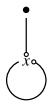
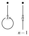
Figure 4: Binding graphs of $\mathit{repeat}$, $\mathit{replicate}$, and the term from Fig. 3

The binding-graph of $\mathit{replicate}$ is very similar featuring the same kind of parameter cycle, only does it involve an additional parameter. Also we have to apply the idea of gβ-reduction when searching upwards from $λx$. First we encounter another abstraction $λn$, which according to the notion of gβ-reduction requires us to leave out the next application node. In the left branch of the multiplexer this is the one with $n-1$ in argument position. Therefore we end up with $x$ as the argument of the matching application node, by which we obtain $x\mathrel{\scriptsize\fourier}x$. Parameter cycles of greater length would occur for scenarios involving mutual recursion such as the term in Fig. 3.

5.2 Inference Rules

To properly define the binding relation we formulate it using inference rules. Since it follows the structure of typing rules, we first give rules for a simply-typed $\lambda_{\textit{letrec}}$-calculus (Fig. 5) and then decorate these typing rules to also yield a term's binding graph, by which we hope to provide an easier access for those who are already familiar with typing rules for the λ-calculus. Type variables are denoted by Greek letters.

Var $$\displaystyle{\hbox{\hskip 18.44608pt\vbox{\hbox{\hskip-18.44606pt\hbox{\hbox{$\displaystyle\displaystyle{x:\tau\in Γ}$}}}\vbox{}}}\over\hbox{\hskip 17.33502pt\vbox{\vbox{}\hbox{\hskip-17.33502pt\hbox{\hbox{$\displaystyle\displaystyle{Γ⇒x:\tau}$}}}}}} \displaystyle{\hbox{\hskip 35.02019pt\vbox{\hbox{\hskip-35.02017pt\hbox{\hbox{$\displaystyle\displaystyle{Γ∪\{x:\tau\}⇒e:\sigma}$}}}\vbox{}}}\over\hbox{\hskip 30.15912pt\vbox{\vbox{}\hbox{\hskip-30.1591pt\hbox{\hbox{$\displaystyle\displaystyle{Γ⇒λx.e:\tau\textrightarrow\sigma}$}}}}}} \displaystyle{\hbox{\hskip 87.46355pt\vbox{\hbox{\hskip-87.46353pt\hbox{\hbox{$\displaystyle\displaystyle{\forall i\in\{0,\dots,n\}:Γ∪\{f_{1}:\tau_{1},\dots,f_{n}:\tau_{n}\}⇒e_{i}:\tau_{i}}$}}}\vbox{}}}\over\hbox{\hskip 81.81056pt\vbox{\vbox{}\hbox{\hskip-81.81056pt\hbox{\hbox{$\displaystyle\displaystyle{Γ⇒\texttt{letrec}~{}f_{1}=e_{1}~{}\dots~{}f_{n}=e_{n}~{}~{}\texttt{in}~{}~{}e_{0}~{}:~{}\tau_{0}}$}}}}}} \displaystyle{\hbox{\hskip 70.8272pt\vbox{\hbox{\hskip-70.8272pt\hbox{\hbox{$\displaystyle\displaystyle{Γ⇒e_{1}:\tau\textrightarrow\sigma\penalty-10000\hskip 20.00003pt plus 0.5fil minus 5.0ptΓ⇒e_{2}:\rho\penalty-10000\hskip 20.00003pt plus 0.5fil minus 5.0pt\tau=\rho}$}}}\vbox{}}}\over\hbox{\hskip 22.88106pt\vbox{\vbox{}\hbox{\hskip-22.88106pt\hbox{\hbox{$\displaystyle\displaystyle{Γ⇒e_{1}~{}e_{2}:\sigma}$}}}}}}$$        Abs        Letrec        App

Figure 5: Typing rules for the simply-typed $\lambda_{\textit{letrec}}$-calculus

In order to infer the binding relation (Fig. 6), at any application $e_{1}~{}e_{2}$ one has to determine to which variable $e_{2}$ might be bound to in $e_{1}$. That we accomplish by annotating the types of terms with the names of the variables that are bound by their abstractions. The annotations are in superscript position, so for some annotated types $x:\tau$, $y:\sigma$, $e_{3}:\rho$, the annotated type of $e_{1}=λx.λy.e_{3}$ is $e_{1}:(\tau\textrightarrow(\sigma\textrightarrow\rho)^{y})^{x}$. We use $\epsilon$ as an annotation to indicate that we cannot determine the associated variable (due to the use of higher-order functions).

The binding relation is denoted on the left-hand side of the turnstile symbol. Both upper-case and lower-case Greek letters denote annotated type variables, but the latter do not include the outermost annotation (which are then added explicitly).

$${\vbox{\hbox{\hbox{\small\sc Var}}\hbox{$\displaystyle\displaystyle{\hbox{\hskip 18.48778pt\vbox{\hbox{\hskip-18.48776pt\hbox{\hbox{$\displaystyle\displaystyle{x:T\in Γ}$}}}\vbox{}}}\over\hbox{\hskip 25.71pt\vbox{\vbox{}\hbox{\hskip-25.70999pt\hbox{\hbox{$\displaystyle\displaystyle{\emptyset\vdash Γ⇒x:T}$}}}}}}$}}}\penalty 50\hskip 20.00003pt plus 0.5fil minus 5.0pt{\vbox{\hbox{\hbox{\small\sc Abs}}\hbox{$\displaystyle\displaystyle{\hbox{\hskip 45.39857pt\vbox{\hbox{\hskip-45.39857pt\hbox{\hbox{$\displaystyle\displaystyle{B\vdash Γ∪\{x:\tau^{\epsilon}\}⇒e:\Sigma}$}}}\vbox{}}}\over\hbox{\hskip 46.02669pt\vbox{\vbox{}\hbox{\hskip-46.02667pt\hbox{\hbox{$\displaystyle\displaystyle{B\vdash Γ⇒λx.e:(\tau^{\epsilon}\textrightarrow\Sigma)^{x}}$}}}}}}$}}}\penalty 50\hskip 20.00003pt plus 0.5fil minus 5.0pt{\vbox{\hbox{\hbox{\small\sc Letrec}}\hbox{$\displaystyle\displaystyle{\hbox{\hskip 101.20767pt\vbox{\hbox{\hskip-101.20766pt\hbox{\hbox{$\displaystyle\displaystyle{\forall i\in\{0,\dots,n\}:B_{i}\vdash Γ∪\{f_{1}:T_{1},\dots,f_{n}:T_{n}\}⇒e_{i}:T_{i}}$}}}\vbox{}}}\over\hbox{\hskip 109.26968pt\vbox{\vbox{}\hbox{\hskip-109.26968pt\hbox{\hbox{$\displaystyle\displaystyle{B_{0}∪\dots∪B_{n}\vdash Γ⇒\texttt{letrec}~{}f_{1}=e_{1}~{}\dots~{}f_{n}=e_{n}~{}~{}\texttt{in}~{}~{}e_{0}~{}:~{}T_{0}}$}}}}}}$}}}\penalty 50\hskip 20.00003pt plus 0.5fil minus 5.0pt{\vbox{\hbox{\hbox{\small\sc App}}\hbox{$\displaystyle\displaystyle{\hbox{\hskip 129.00815pt\vbox{\hbox{\hskip-129.00815pt\hbox{\hbox{$\displaystyle\displaystyle{B_{1}\vdash Γ⇒e_{1}:(T\textrightarrow\Sigma)^{x}\penalty-10000\hskip 20.00003pt plus 0.5fil minus 5.0ptB_{2}\vdash Γ⇒e_{2}:R\penalty-10000\hskip 20.00003pt plus 0.5fil minus 5.0ptbare(T)=bare(R)}$}}}\vbox{}}}\over\hbox{\hskip 101.72905pt\vbox{\vbox{}\hbox{\hskip-101.72905pt\hbox{\hbox{$\displaystyle\displaystyle{B_{1}∪B_{2}∪bind(x,e_{2})∪blackholes(R)\vdash Γ⇒e_{1}~{}e_{2}:\Sigma}$}}}}}}$}}}\penalty 50\hskip 20.00003pt plus 0.5fil minus 5.0ptblackholes(T)=\begin{cases}blackholes(R)∪\{x\mathrel{\scriptsize\fourier}\bullet\}&\text{if $T=(\Sigma\textrightarrow R)^{x}$}\\ blackholes(R)&\text{if $T=(\Sigma\textrightarrow R)^{\epsilon}$}\\ \emptyset&\text{otherwise}\end{cases}\penalty 50\hskip 20.00003pt plus 0.5fil minus 5.0ptbind(x,e_{2})=\begin{cases}\emptyset&\text{if $x=\epsilon$}\\ \{x\mathrel{\scriptsize\fourier}e_{2}\}&\text{otherwise}\end{cases}\penalty 50\hskip 20.00003pt plus 0.5fil minus 5.0pt$$

Figure 6: Inductive definition of the binding relation based on annotated types

In the Abs rule the abstraction puts a new variable $x$, which is annotated by an $\epsilon$ because we do not make assumptions on the variables exposed by higher-order functions. The type of $λx.e$ is annotated by $x$, which is exposed. To compare types App employs a function $bare:A\textrightarrow T$, which maps annotated types $A$ to bare types $T$ by removing all annotations. Two further functions, $bind$ and $blackholes$, are used to enumerate the elements to be added to the binding relation. In case the argument $e_{2}$ is a higher-order function the expressions cannot be determined that are bound to the variables it exposes, therefore $blackholes$ binds a blackhole to each of them.

Proposition 7

Every derivation ${\cal D}$ in the type system in Fig. 5 with conclusion $\emptyset\Rightarrow M:\tau$, which justifies the assignment of type $\tau$ to the $\lambda_{\textit{letrec}}$-term $M$, can be decorated effectively with as result a derivation $\tilde{{\cal D}}$ in the proof system in Fig. 6 with conclusion $B\vdash\emptyset\Rightarrow M:\tilde{\tau}$, by which the binding graph $B$ for $M$ is obtained and justified.

The proof of this proposition consists in describing an effective algorithm that, given a derivation ${\cal D}$ in the type system in Fig. 5, proceeds as follows: First it constructs, in a step by step manner, variable decorations for the types in ${\cal D}$ (by concentrating on `spine loops' of $M$ that correspond to cyclic threads in ${\cal D}$, and starting with the decorations at formulas on such threads where the types have minimal length) in such a way that the rule instances are correct for the system in Fig. 6 when the leading binding graph annotations of the form $B\vdash$ are neglected. Second, after the first step is concluded, the algorithm constructs the binding graph annotations according to the rules in Fig. 6 in a top-down manner.

6 Transformation

Using the binding graph we will now develop a more general version of the optimisation previously formulated as rewriting rules restricted to directly recursive functions.

An edge $x\mathrel{\scriptsize\fourier}e$ in the binding graph of a term $t$ indicates a (possibly infinite) class of gβ-redexes on the infinite unfolding $T$ of $t$. While all these redexes could be at once contracted on $T$ this does not automatically carry over to its finite representation $t$. Let us for the present restrict our attention to cases where $x$ has no further incoming edges.

Proposition 8

Let $t$ be a $\lambda_{\textit{letrec}}$-term with infinite unfolding $T$ and a binding graph featuring a node $x$ with a single incoming edge $x\mathrel{\scriptsize\fourier}e$. If we label the transition that contracts all gβ-redexes with involving a $λx$-abstraction $red$, and the substitution of all occurrences of $t$ by $e$ and the subsequent elimination of all vacuous $λx$-abstractions $trans$, then the following diagram commutes.

$$\begin{array}[]{rcl}t&{\twoheadrightarrow\twoheadrightarrow}_{\medtriangledown}&T\\ trans\textdownarrow&&\textdownarrow red\\ t^{\prime}&{\twoheadrightarrow\twoheadrightarrow}_{\medtriangledown}&T^{\prime}\end{array}$$

This follows from the following considerations. Since we assume unique variable naming, the infinitely unfolding $t$ without any renaming is semantics preserving. [9] Every occurrence of $λv$ in $t$ gives rise to one ore more gβ-redexes in $T$ each having $λv$ with $p$ as an argument. This follows from $x\mathrel{\scriptsize\fourier}e$ being the sole incoming edge of $x$. By both paths from $t$ to $T^{\prime}$ one finds $T^{\prime}$ to have the same shape: There are no occurrences of neither $λx$ nor $x$. Evidently this not a very strong argument and we hope to improve on it by means of higher-order reasoning.

The restriction above to only consider nodes with a single predecessor prevents us from dealing with any of the examples shown so far since they involve cyclic binding graphs. Fortunately, it can be relaxed to a much less restrictive property.

Definition 9 (Domination, and strong domination)

Let a $G=\langle{V},\hskip 0.5pt{{\rightarrowtail}}\rangle$ be a directed graph, and $u$ and $v$ be vertices of $G$. We say that $v$ dominates $w$ ($v$ is a dominator for $w$, symbolically: ${{{\mit dom}_{G}}}({v,w})$) if either $v=w$ or $v\neq w$ and for every path $\pi$ in $G$ that leads to $w$ but does not contain $v$ it holds that the start vertex of $\pi$ is reachable from $v$; more formally, if:

$$v=w\,\,\vee\,\,\bigl{(}\,v\neq w\,\,\land\,\,\forall u_{0},\ldots,u_{n}\in V\setminus\{v\}\bigl{[}\,u_{0}\mathrel{{\rightarrowtail}}u_{1}\mathrel{{\rightarrowtail}}\ldots\mathrel{{\rightarrowtail}}u_{n}=w\,\,\Longrightarrow\,\,v\mathrel{{\rightarrowtail^{*}}}u_{0}\,\bigr{]}\bigr{)}$$ (1)

Note that $v\mathrel{{\rightarrowtail^{*}}}w$ holds if $v$ dominates $w$.

And we say that $v$ strongly dominates $w$ ($v$ is a strong dominator for $w$, symbolically: ${{{\mit sdom}_{G}}}({v,w})$) if $v\neq w$ and for every path $\pi$ in $G$ that leads to $w$ but does not contain $v$ it holds that the start vertex $u_{0}$ of $\pi$ is reachable from $v$, but does not reside on a common cycle with $v$, more formally, if:

$$v\neq w\,\,\land\,\,\forall u_{0},\ldots,u_{n}\in V\setminus\{v\}\bigl{[}\,u_{0}\mathrel{{\rightarrowtail}}u_{1}\mathrel{{\rightarrowtail}}\ldots\mathrel{{\rightarrowtail}}u_{n}=w\,\,\Longrightarrow\,\,v\mathrel{{\rightarrowtail^{*}}}u_{0}\,\,\,\land\,\,\,u_{0}\mathrel{{{\not\rightarrowtail}^{*}}}v\,\bigr{]}$$ (2)

Remark 10

The standard definition of a `$v$ dominates $w$' for control-flow graphs (see e.g. [10]) requires that each path from the start node to $w$ has to pass through $v$. The definition above is a generalisation to directed graphs that does not depend on the existence of a designated start node. Our definition of `$v$ strongly dominates $w$' excludes self-domination (i.e. makes the relation irreflexive), and adds the restriction that for all paths from $v$ to $w$ that do not repeatedly pass through $v$ it holds no vertex except the starting vertex $v$ resides on a common cycle with $v$.

The following proposition suggests an alternative, co-recursive definition of strong domination between vertices, which proceeds stepwisely by examining predecessors of the strongly dominated vertex.

Proposition 11

Let $G=\langle{V},\hskip 0.5pt{{\rightarrowtail}}\rangle$ be a directed graph. Then for all $v,w\in V$ it holds:

$${{{\mit sdom}_{G}}}({v,w})\,\,\Longleftrightarrow\,\,v\neq w\,\,\land\,\,{v}\mathrel{{\rightarrowtail^{+}}}{w}\,\,\land\,\,{w}\mathrel{{{\not\rightarrowtail}^{+}}}{v}\,\,\land\,\,\forall u\in V\bigl{(}\,u\mathrel{{\rightarrowtail}}w\,\,\land\,\,u\neq v\Rightarrow{{{\mit sdom}_{G}}}({v,u})\,\bigr{)}$$

For the definition of the optimising transformation, we choose a formulation different from the one using rewrite rules described in Section 4, one that is particularly easy to express. Such as β-reduction can be decomposed into substitution of individual occurrences of variables (local β-reduction) and the elimination of vacuous bindings (AT-removal) as described in [5], for the transformation we have the possibility of expressing the transformation with an arbitrary level of granularity. The following rule encompasses the substitution of all occurrences of one dominated variable. It could have been formulated more fine-grained by substituting only individual occurrences, or less fine-grained by including the elimination of the bindings that have become vacuous.

Proposition 12 (Main proposition)

In a $\lambda_{\textit{letrec}}$-term $t$ occurrences of a variable that is dominated by an expression $d$ in $t$'s binding graph can be substituted by $d$.

$$\displaystyle{\hbox{\hskip 67.86612pt\vbox{\hbox{\hskip-67.86612pt\hbox{\hbox{$\displaystyle\displaystyle{B\vdash\emptyset⇒t:\Sigma\qquad B⇒dom_{B}(d,x)}$}}}\vbox{}}}\over\hbox{\hskip 29.09335pt\vbox{\vbox{}\hbox{\hskip-29.09334pt\hbox{\hbox{$\displaystyle\displaystyle{t=^{\infty}_{\medtriangledown,g\beta}t\langle x:=d\rangle}$}}}}}}$$

7 Advanced Examples

There are interesting examples to which the presented transformation cannot be directly applied or does not lead to satisfactory results. Only in combination with a number well-directed unfoldings the desired effect can be obtained. Let us consider two schematic examples:

The first one exhibits dominated parameters only after a single let-unfolding (Fig. 7). Also it features repetitive reduction pattern, without having a parameter cycle. This because the argument in question is bound outside of the recursion. Still, after the unfolding the presented optimisation does cure the term.

               $\mathrel{\rightarrow_{\medtriangledown}}$               

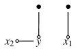
Figure 7: A term, which after one unfolding exhibits a dominated parameter

The second of the two term is particularly intricate since it can be unfolded and then transformed in many different ways with considerable differences in the amount of concealed gβ-redexes. Most solutions involve more than one recursive call with more than two arguments. The ideal transformation with respect to the number of concealed redexes of both terms is depicted in Fig. 8.

$=^{\infty}_{\medtriangledown,g\beta}$ $=^{\infty}_{\medtriangledown,g\beta}$

Figure 8: Optimisation of two terms that are not covered by the presented rewriting rules

8 Status quo

Presently this work consists mostly of an extended problem description, which is to a some extent rather informal. Ideas for resolution have been presented, but yet lack both precision and genericity. Therefore, outstanding issues to continue the investigation suggest themselves. Currently we are working on the following problems:

• Properly formalising the concepts introduced in this report. This involves putting grammars and rewrite rules into the higher-order setting of HRSs.

• Investigate whether there are other interesting notions of `operational equivalence', apart from applicative bisimulation, with respect to which we could show correctness of our optimising transformation. (We think of notions that are in line with the semantics of functional programming languages, but nevertheless are language independent, and also of theoretical interest.)

• Expressing the presented transformation as a higher-order rewrite system and proving its correctness with respect to that equivalence relation.

Once these fundamental issues are resolved, we intend to tackle the following questions:

• We have seen that unfolding a $\lambda_{\textit{letrec}}$-term in order to facilitate the optimisation can be effected in different ways, leading to terms of different quality. To obtain the most efficient terms one has to provide a procedure to select the most suitable unfolding for each situation.

• This requires an adequate measure for efficiency.

• We would like to learn more about the rewrite properties of the transformation: is it possible to find a formulation that guarantees confluence and normalisation?

• In some of the easy examples we studied, our transformation seemed to be closely connected with the concept of `lambda-dropping' [8, 6], and hence also with its converse, `lambda-lifting' [11, 13, 7]. We want to understand that relationship in detail.

• Once the analysis has been optimised in terms of genericity, i.e. that it recognises as many cases as possible for which the transformation is correct, it would be interesting to assess the frequency in which these cases occur in existing systems, such as functional programming libraries or intermediate code generated by compilers.

• The remaining question is, how the optimisation actually affects the run-time efficiency of real-world systems like Haskell programs.

Acknowledgment.

The incentive to investigate the presented optimisation was provided by Doaitse Swierstra. We thank him and Vincent van Oostrom for many insightful discussions and hints.

References

- [1]
- [2] Samson Abramsky (1990): The Lazy Lambda Calculus. In: Research Topics in Functional Programming. Addison-Wesley, pp. 65–116. Updated version (2006) available at http://web.comlab.ox.ac.uk/people/Samson.Abramsky/lazy.pdf.
- [3] Andrea Asperti & Stefano Guerrini (1998): The Optimal Implementation of Functional Programming Languages. Cambridge Tracts in Theoretical Computer Science 45, Cambridge University Press.
- [4] H.P. Barendregt (1984): The Lambda Calculus: Its Syntax and Semantics, nd edition. SLFM 103, Elsevier.
- [5] N.G. de Bruijn (1987): Generalizing Automath by Means of a Lambda-Typed Lambda Calculus. Technical Report AUT092 (AUTOMATH archive http://www.win.tue.nl/automath/), Technische Universiteit Eindhoven, Eindhoven, the Netherlands. Available at http://alexandria.tue.nl/repository/freearticles/597608.pdf.
- [6] Olivier Danvy (1999): An Extensional Characterization of Lambda-Lifting and Lambda-Dropping. In Aart Middeldorp & Taisuke Sato, editors: Functional and Logic Programming. LNCS 1722, Springer Berlin / Heidelberg, pp. 241–250, 10.1007/10705424_16.
- [7] Olivier Danvy & Ulrik Schultz (2002): Lambda-Lifting in Quadratic Time. In Zhenjiang Hu & Mario Rodríguez-Artalejo, editors: Functional and Logic Programming. LNCS 2441, Springer Berlin / Heidelberg, pp. 134–151, 10.1007/3-540-45788-7_8.
- [8] Olivier Danvy & Ulrik P. Schultz (1997): Lambda-dropping: transforming recursive equations into programs with block structure. In: Proceedings of the 1997 ACM SIGPLAN symposium on Partial evaluation and semantics-based program manipulation. PEPM '97, ACM, New York, NY, USA, pp. 90–106, 10.1145/258993.259007.
- [9] Jörg Endrullis, Clemens Grabmayer, Jan Willem Klop & Vincent van Oostrom (2010): On Equal -Terms. Submitted, currently under review, to be published in 2011.
- [10] M. S. Hecht & J. D. Ullman (1974): Characterizations of Reducible Flow Graphs. JACM 21, pp. 367–375, 10.1145/321832.321835.
- [11] Thomas Johnsson (1985): Lambda lifting: Transforming programs to recursive equations. In Jean-Pierre Jouannaud, editor: Functional Programming Languages and Computer Architecture. LNCS 201, Springer Berlin / Heidelberg, pp. 190–203, 10.1007/3-540-15975-4_37.
- [12] Fairouz Kamareddine & Rob Nederpelt (1995): Refining reduction in the lambda calculus. Journal of Functional Programming 5(4), pp. 637–651, 10.1017/S0956796800001507.
- [13] Simon L. Peyton Jones (1987): The Implementation of Functional Programming Languages (Prentice-Hall International Series in Computer Science). Prentice-Hall, Inc., Upper Saddle River, NJ, USA.
- [14] Terese (2003): Term Rewriting Systems. Cambridge Tracts in Theoretical Computer Science 55, Cambridge University Press.