Estimating and understanding exponential random graph models

Abstract

We introduce a method for the theoretical analysis of exponential random graph models. The method is based on a large-deviations approximation to the normalizing constant shown to be consistent using theory developed by Chatterjee and Varadhan [European J. Combin. 32 (2011) 1000–1017]. The theory explains a host of difficulties encountered by applied workers: many distinct models have essentially the same MLE, rendering the problems “practically” ill-posed. We give the first rigorous proofs of “degeneracy” observed in these models. Here, almost all graphs have essentially no edges or are essentially complete. We supplement recent work of Bhamidi, Bresler and Sly [2008 IEEE 49th Annual IEEE Symposium on Foundations of Computer Science (FOCS) (2008) 803–812 IEEE] showing that for many models, the extra sufficient statistics are useless: most realizations look like the results of a simple Erdős–Rényi model. We also find classes of models where the limiting graphs differ from Erdős–Rényi graphs. A limitation of our approach, inherited from the limitation of graph limit theory, is that it works only for dense graphs.

and

t1Supported in part by NSF Grant DMS-10-05312 and a Sloan Research Fellowship.

t2Supported in part by NSF Grant DMS-08-04324.

62F10, 05C80, 62P25, 60F10, Random graph, Erdos–Renyi, graph limit, exponential random graph models, parameter estimation

1 Introduction

Graph and network data are increasingly common and a host of statistical methods have emerged in recent years. Entry to this large literature may be had from the research papers and surveys in Fienberg fienberg , fienberg2 . One mainstay of the emerging theory are the exponential families

$$p_{\beta}(G)=\exp\Biggl{(}\sum_{i=1}^{k}\beta_{i}T_{i}(G)-\psi(\beta)\Biggr{)},$$ (1)

where $\beta=(\beta_{1},\ldots,\beta_{k})$ is a vector of real parameters, $T_{1},T_{2},\ldots,T_{k}$ are functions on the space of graphs (e.g., the number of edges, triangles, stars, cycles$,\ldots$), and $\psi$ is the normalizing constant. In this paper, $T_{1}$ is usually taken to be the number of edges (or a constant multiple of it).

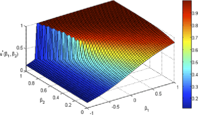
Figure 1: The plot of $u^{*}$ against $(\beta_{1},\beta_{2})$. There is a discontinuity on the left where $u^{*}$ jumps from near $0$ to near $1$; this corresponds to a phase transition. (Picture by Sukhada Fadnavis.)

We review the literature of these models in Section 2.1. Estimating the parameters in these models has proved to be a challenging task. First, the normalizing constant $\psi(\beta)$ is unknown. Second, very different values of $\beta$ can give rise to essentially the same distribution on graphs.

Here is an example: consider the model on simple graphs with $n$ vertices,

$$p_{\beta_{1},\beta_{2}}(G)=\exp\biggl{(}2\beta_{1}E+\frac{6\beta_{2}}{n}\Delta-n^{2}\psi_{n}(\beta_{1},\beta_{2})\biggr{)},$$ (2)

where $E$, $\Delta$ denote the number of edges and triangles in the graph $G$. The normalization of the model ensures nontrivial large $n$ limits. Without scaling, for large $n$, almost all graphs are empty or full. This model is studied by Strauss strauss , Park and Newman park04 , park05 , Häggstrom and Jonasson hj99 , and many others.

Theorems 3.1 and 4.1 will show that for $n$ large and nonnegative $\beta_{2}$,

$$\quad\psi_{n}(\beta_{1},\beta_{2})\simeq\sup_{0\leq u\leq 1}\biggl{(}\beta_{1}u+\beta_{2}u^{3}-\frac{1}{2}u\log u-\frac{1}{2}(1-u)\log(1-u)\biggr{)}.$$ (3)

The maximizing value of the right-hand side is denoted $u^{*}(\beta_{1},\beta_{2})$. A plot of this function appears in Figure 1. Theorem 4.2 shows that for any $\beta_{1}\in\mathbb{R}$ and $\beta_{2}>0$, with high probability, a pick from $p_{\beta_{1},\beta_{2}}$ is essentially the same as an Erdős–Rényi graph generated by including edges independently with probability $u^{*}(\beta_{1},\beta_{2})$. This phenomenon has previously been identified by Bhamidi et al. bhamidi and is discussed further in Section 2.1. Figure 2 shows the contour lines for Figure 1. All the $(\beta_{1},\beta_{2})$ values on the same contour line lead to the same Erdős–Rényi model in the limit.

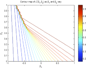
Figure 2: Contour lines for Figure 1. All pairs $(\beta_{1},\beta_{2})$ on the same contour line correspond to the same value of $u^{*}$ and hence those models will correspond to the same Erdős–Rényi model in the limit. The phase transition region is seen in the upper left-hand corner where all contour lines converge. (Picture by Sukhada Fadnavis.)

Our development uses the emerging tools of graph limits as developed by Lovász and coworkers. We give an overview in Section 2.2. Briefly, a sequence of graphs $G_{n}$ converges to a limit if the proportion of edges, triangles, and other small subgraphs in $G_{n}$ converges. There is a limiting object and the space of all these limiting objects serves as a useful compactification of the set of all graphs. Our theory works for functions $T_{i}(G)$ which are continuous in this topology. In their study of the large deviations of Erdős–Rényi random graphs, Chatterjee and Varadhan cv10 derived the associated rate functions in the language of graph limit theory. Their work is crucial in the present development and is reviewed in Section 2.3.

Our main results are in Section 3 through Section 7. These sections contain only the statements of the theorems; all proofs are given in Section 8.

Working with general exponential models, Section 3 gives an extension of the approximation (3) for $\psi_{n}$ (Theorem 3.1) and shows that, in the limit, almost all graphs from the model (1) are close to graphs where a certain functional is maximized. As will emerge, sometimes this maximum is taken on at a unique Erdős–Rényi model.

The main statistical motivation of this paper comes from the formula for the limit of the normalizing constant given in Theorem 3.1, since the normalizing constant is crucial for the computation of maximum likelihood estimates. At present, the computational tools used by practitioners to compute the normalizing constants in exponential random graph models become prohibitively time-consuming even for moderately large $n$. The theory initiated in this paper hopes to circumvent this problem by providing analytical formulas. As mentioned in the abstract, the limitation of our approach is that as of now, it applies only to dense graphs.

Incidentally, in a recent meeting at the American Institute of Mathematics, computer-intensive calculations carried out by Mark Handcock and David Hunter indicated that the formula given in Theorem 3.1 is actually a pretty good approximation to the exact value of the normalizing constant even for $n$ as small as 20.

Section 4 studies the problem for the model (1) when $\beta_{2},\ldots,\beta_{k}$ are positive ($\beta_{1}$ may have any sign). When the $T_{i}$’s are subgraph counts, positive $\beta_{i}$’s were originally intentioned (e.g., in frank ) to “encourage” the presence of the corresponding subgraphs. It is shown that the large-deviations approximation for $\psi_{n}$ can be easily calculated as a one-dimensional maximization (Theorem 4.1). Further, amplifying the results of Bhamidi et al. bhamidi , it is shown that in these cases, almost all realizations of the model (1) are close to an Erdős–Rényi graph (or perhaps a finite mixture of Erdős–Rényi graphs) (Theorem 4.2). These mixture cases actually occur for natural parameter values. Section 5 also gives a careful account of the phase transitions and near-degeneracies observed in the edge-triangle model (3).

Sections 6 and 7 investigate cases where $\beta_{i}$ is allowed to be negative. While the general case remains open (and appears complicated), in Section 6 it is shown that Theorems 4.1 and 4.2 hold as stated if $(\beta_{i})_{2\leq i\leq k}$ are sufficiently small in magnitude. This requires a careful study of associated Euler–Lagrange equations. Section 7 shows how the results change for the model containing edges and triangles when $\beta_{2}$ is negative. For sufficiently large negative $\beta_{2}$, typical realizations look like a random bipartite graph (where “random” means that the two parts, of equal size, are chosen uniformly at random from all possible choices). This is very different from the Erdős–Rényi model. The result generalizes to other models via an interesting analogy with the Erdős–Stone theorem from extremal graph theory.

A longer version of this paper with more pictures and additional results is available as “version 3” on arXiv (http://arxiv.org/pdf/1102.2650v3.pdf).

2 Background

This section gives needed background and notation in three areas. Exponential graph models (Section 2.1), graph limits (Section 2.2), and large deviations (Section 2.3).

2.1 Exponential random graphs

Let $\mathcal{G}_{n}$ be the space of all simple graphs on $n$ labeled vertices (“simple” means undirected, with no loops or multiple edges). Thus, $\mathcal{G}_{n}$ contains $2^{{n\choose 2}}$ elements. A variety of models in active use can be presented in exponential form

$$p_{\beta}(G)=\exp\Biggl{(}\sum_{i=1}^{k}\beta_{i}T_{i}(G)-\psi(\beta)\Biggr{)},$$ (4)

where $\beta=(\beta_{1},\ldots,\beta_{k})$ is a vector of real parameters, $T_{1},T_{2},\ldots,T_{k}$ are real-valued functions on $\mathcal{G}_{n}$, and $\psi(\beta)$ is a normalizing constant. Usually, $T_{i}$ are taken to be counts of various subgraphs, for example, $T_{1}(G)=\#$ edges in $G$, $T_{2}(G)=\#$ triangles in $G,\ldots\,$. The main results of Section 3 work for more general “continuous functions” on graph space, such as the degree sequence or the eigenvalues of the adjacency matrix. This allows models with sufficient statistics of the form $\sum_{i=1}^{n}\beta_{i}d_{i}(G)$ with $d_{i}(G)$ the degree of vertex $i$. See, for example, pd177 .

These exponential models were used by Holland and Leinhardt holland in the directed case. Frank and Strauss frank developed them, showing that if $T_{i}$ are chosen as edges, triangles, and stars of various sizes, the resulting random graph edges form a Markov random field. A general development is in Wasserman and Faust wasserman . Newer developments, consisting mainly of new sufficient statistics and new ranges for parameters that give interesting and practically relevant structures, are summarized in Snijders et al. snijders06 . Finally, Rinaldo et al. rinaldo develop the geometric theory for this class of models with extensive further references.

A major problem in this field is the evaluation of the constant $\psi(\beta)$ which is crucial for carrying out maximum likelihood and Bayesian inference. As far as we know, there is no feasible analytic method for approximating $\psi$ when $n$ is large. Physicists have tried the technique of mean-field approximations; see Park and Newman park04 , park05 for the case where $T_{1}$ is the number of edges and $T_{2}$ is the number of two-stars or the number of triangles. Mean-field approximations have no rigorous foundation, however, and are known to be unreliable in related models such as spin glasses talagrand03 . For exponential graph models, Chatterjee and Dey chatterjeedey10 prove that they work for some restricted ranges of $\{\beta_{i}\}$: values where the graphs are shown to be essentially Erdős–Rényi graphs (see Theorem 4.2 below and bhamidi ).

A host of techniques for approximating the normalizing constant using various Monte Carlo schemes have been proposed. These include the MCMLE procedure of Geyer and Thompson gt92 . The bridge sampling approach of Gelman and Meng gelman also builds on techniques suggested by physicists to estimate free energy [$\psi(\beta)$ in our context]. The equi-energy sampler of Kou et al. kou can also be harnessed to estimate $\psi$.

Alas, at present writing these procedures seem useful only for relatively small graphs. For bigger graphs, the run-time of the Monte Carlo algorithms become unpleasantly long. Snijders snijders09 and Handcock handcock demonstrate this empirically with further discussion in snijders06 . One theoretical explanation for the poor performance of these techniques comes from the work of Bhamidi et al. bhamidi . Most of the algorithms above require a sample from the model (4). This is most often done by using a local Markov chain based on adding or deleting edges via Metropolis or Glauber dynamics (Gibbs sampling). These authors show that if the parameters are nonnegative, then for large $n$,

• either the $p_{\beta}$ model is essentially the same as an Erdős–Rényi model (in which case the Markov chain mixes in $n^{2}\log n$ steps);

• or the Markov chain takes exponential time to mix.

Thus, in cases where the model is not essentially trivial, the Markov chains required to carry MCMLE procedures cannot be usefully run to stationarity.

Two other approaches to estimation are worth mentioning. The pseudo-likelihood approach of Besag besag75 is widely used because of its ease of implementation. Its properties are at best poorly understood: it does not directly maximize the likelihood and in empirical comparisions (see, e.g., corander ), has appreciably larger variability than the MLE. Comets and Janžura cj98 prove consistency and asymptotic normality of the maximum pseudo-likelihood estimator in certain Markov random field models. Chatterjee chatterjee07 shows that it is consistent for estimating the temperature parameter of the Sherrington–Kirkpatrick model of spin glasses. The second approach is Snijders’ snijders09 suggestion to use the Robbins–Monro optimization procedure rm51 to compute solutions to the moment equations $E_{\beta}(T(G))=T(G^{*})$ where $G^{*}$ is the observed graph. While promising, the approach requires generating points from $p_{\beta}$ for arbitrary $\beta$. The only way to do this at present is by MCMC and the results of bhamidi suggest this may be impractical.

2.2 Graph limits

In a sequence of papers borgsetal06 , borgsetal08 , borgsetal07 , freedmanlovaszschrijver07 , lovasz06 , lovasz07 , lovaszsos08 , lovaszszegedy06 , lovaszszegedy07 , lovaszszegedy07b , lovaszszegedy09 , Laszlo Lovász and coauthors V. T. Sós, B. Szegedy, C. Borgs, J. Chayes, K. Vesztergombi, A. Schrijver, and M. Freedman have developed a beautiful, unifying theory of graph limits. (See also the related work of Austin austin08 and Diaconis and Janson pd175 which traces this back to work of Aldous aldous81 , Hoover hoover82 and Kallenberg kallenberg05 .) This body of work sheds light on various graph-theoretic topics such as graph homomorphisms, Szemerédi’s regularity lemma, quasi-random graphs, graph testing and extremal graph theory, and has even found applications in statistics and related areas (see, e.g., pd177 ). Their theory has been developed for dense graphs (number of edges comparable to the square of number of vertices) but parallel theories for sparse graphs are beginning to emerge bollobasriordan09 .

Lovász and coauthors define the limit of a sequence of dense graphs as follows. We quote the definition verbatim from lovaszszegedy06 (see also borgsetal08 , borgsetal07 , pd175 ). Let $G_{n}$ be a sequence of simple graphs whose number of nodes tends to infinity. For every fixed simple graph $H$, let $|{\hom(H,G)}|$ denote the number of homomorphisms of $H$ into $G$ [i.e., edge-preserving maps $V(H)\to V(G)$, where $V(H)$ and $V(G)$ are the vertex sets]. This number is normalized to get the homomorphism density

$$t(H,G):=\frac{|{\hom(H,G)}|}{|V(G)|^{|V(H)|}}.$$ (5)

This gives the probability that a random mapping $V(H)\to V(G)$ is a homomorphism.

Note that $|{\hom(H,G)}|$ is not the count of the number of copies of $H$ in $G$, but is a constant multiple of that if $H$ is a complete graph. For example, if $H$ is a triangle, $|{\hom(H,G)}|$ is the number of triangles in $G$ multiplied by six. On the other hand if $H$ is, say, a $2$-star (i.e., a triangle with one edge missing) and $G$ is a triangle, then the number of copies of $H$ in $G$ is zero, while $|{\hom(H,G)}|=3^{3}=27$.

Suppose that the graphs $G_{n}$ become more and more similar in the sense that $t(H,G_{n})$ tends to a limit $t(H)$ for every $H$. One way to define a limit of the sequence $\{G_{n}\}$ is to define an appropriate limit object from which the values $t(H)$ can be read off.

The main result of lovaszszegedy06 (following the earlier equivalent work of Aldous aldous81 and Hoover hoover82 ) is that indeed there is a natural “limit object” in the form of a function $h\in\mathcal{W}$, where $\mathcal{W}$ is the space of all measurable functions from $[0,1]^{2}$ into $[0,1]$ that satisfy $h(x,y)=h(y,x)$ for all $x,y$.

Conversely, every such function arises as the limit of an appropriate graph sequence. This limit object determines all the limits of subgraph densities: if $H$ is a simple graph with $V(H)=[k]=\{1,\ldots,k\}$, let

$$t(H,h)=\int_{[0,1]^{k}}\prod_{\{i,j\}\in E(H)}h(x_{i},x_{j})\,dx_{1}\cdots dx_{k}.$$ (6)

Here $E(H)$ denotes the edge set of $H$. A sequence of graphs $\{G_{n}\}_{n\geq 1}$ is said to converge to $h$ if for every finite simple graph $H$,

$$\lim_{n\to\infty}t(H,G_{n})=t(H,h).$$ (7)

Intuitively, the interval $[0,1]$ represents a “continuum” of vertices, and $h(x,y)$ denotes the probability of putting an edge between $x$ and $y$. For example, for the Erdős–Rényi graph $G(n,p)$, if $p$ is fixed and $n\to\infty$, then the limit graph is represented by the function that is identically equal to $p$ on $[0,1]^{2}$. Clearly, this framework is therefore useful only when $p$ does not tend to zero when $n\rightarrow\infty$, that is, in the case of dense Erdős–Rényi graphs.

These limit objects, that is, elements of $\mathcal{W}$, are called “graph limits” or “graphons” in lovaszszegedy06 , borgsetal08 , borgsetal07 . A finite simple graph $G$ on $\{1,\ldots,n\}$ can also be represented as a graph limit $f^{G}$ is a natural way, by defining

$$f^{G}(x,y)=\cases{1,&\quad if $\bigl{(}\lceil nx\rceil,\lceil ny\rceil\bigr{)}$ is an edge in $G$,\cr 0,&\quad otherwise.}$$ (8)

The definition makes sense because $t(H,f^{G})=t(H,G)$ for every simple graph $H$ and therefore the constant sequence $\{G,G,\ldots\}$ converges to the graph limit $f^{G}$. Note that this allows all simple graphs, irrespective of the number of vertices, to be represented as elements of a single abstract space, namely $\mathcal{W}$.

With the above representation, it turns out that the notion of convergence in terms of subgraph densities outlined above can be captured by an explicit metric on $\mathcal{W}$, the so-called cut distance (originally defined for finite graphs by Frieze and Kannan friezekannan99 ). Start with the space $\mathcal{W}$ of measurable functions $f(x,y)$ on $[0,1]^{2}$ that satisfy $0\leq f(x,y)\leq 1$ and $f(x,y)=f(y,x)$. Define the cut distance

$$d_{\square}(f,g):=\sup_{S,T\subseteq[0,1]}\biggl{|}\int_{S\times T}\bigl{[}f(x,y)-g(x,y)\bigr{]}\,dx\,dy\biggr{|}.$$ (9)

Introduce in $\mathcal{W}$ an equivalence relation: let $\Sigma$ be the space of measure preserving bijections $\sigma\dvtx[0,1]\to[0,1]$. Say that $f(x,y)\sim g(x,y)$ if $f(x,y)=g_{\sigma}(x,y):=g(\sigma x,\sigma y)$ for some $\sigma\in\Sigma$. Denote by ${\widetilde{g}}$ the closure in $(\mathcal{W},d_{\Box})$ of the orbit $\{g_{\sigma}\}$. The quotient space is denoted by $\widetilde{\mathcal{W}}$ and $\tau$ denotes the natural map $g\to{\widetilde{g}}$. Since $d_{\Box}$ is invariant under $\sigma$ one can define on $\widetilde{\mathcal{W}}$, the natural distance $\delta_{\Box}$ by

$$\delta_{\Box}({\widetilde{f}},{\widetilde{g}}):=\inf_{\sigma}d_{\Box}(f,g_{\sigma})=\inf_{\sigma}d_{\Box}(f_{\sigma},g)=\inf_{\sigma_{1},\sigma_{2}}d_{\Box}(f_{\sigma_{1}},g_{\sigma_{2}})$$

making $(\widetilde{\mathcal{W}},\delta_{\Box})$ into a metric space. To any finite graph $G$, we associate $f^{G}$ as in (8) and its orbit ${\widetilde{G}}=\tau f^{G}={\widetilde{f}}^{G}\in\widetilde{\mathcal{W}}$.

The papers by Lovász and coauthors establish many important properties of the metric space $\widetilde{\mathcal{W}}$ and the associated notion of graph limits. For example, $\widetilde{\mathcal{W}}$ is compact. A pressing objective is to understand what functions from $\widetilde{\mathcal{W}}$ into $\mathbb{R}$ are continuous. Fortunately, it is an easy fact that the homomorphism density $t(H,\cdot)$ is continuous for any finite simple graph $H$ borgsetal07 , borgsetal08 . There are other, more complicated functions that are continuous. For example, the degree distribution is continuous with respect to this topology, as is the distribution of eigenvalues. See austin10 , austin08 for further discussions.

2.3 Large deviations for random graphs

Let $G(n,p)$ be the random graph on $n$ vertices where each edge is added independently with probability $p$. This model has been the subject of extensive investigations since the pioneering work of Erdős and Rényi erdosrenyi60 , yielding a large body of literature (see bollobas01 , JLR00 for partial surveys).

Recently, Chatterjee and Varadhan cv10 formulated a large deviation principle for the Erdős–Rényi graph, in the same way as Sanov’s theorem sanov61 gives a large deviation principle for an i.i.d. sample. The formulation and proof of this result makes extensive use of the properties of the topology described in Section 2.2.

Let $I_{p}\dvtx[0,1]\to\mathbb{R}$ be the function

$$I_{p}(u):=\frac{1}{2}u\log\frac{u}{p}+\frac{1}{2}(1-u)\log\frac{1-u}{1-p}.$$ (10)

The domain of the function $I_{p}$ can be extended to $\mathcal{W}$ as

$$I_{p}(h):=\int_{0}^{1}\int_{0}^{1}I_{p}\bigl{(}h(x,y)\bigr{)}\,dx\,dy.$$ (11)

The function $I_{p}$ can be defined on $\widetilde{\mathcal{W}}$ by declaring $I_{p}(\widetilde{h}):=I_{p}(h)$ where $h$ is any representative element of the equivalence class $\widetilde{h}$. Of course, this raises the question whether $I_{p}$ is well defined on $\widetilde{\mathcal{W}}$. It was proved in cv10 that the function $I_{p}$ is indeed well defined on $\widetilde{\mathcal{W}}$ and is lower semicontinuous under the cut metric $\delta_{\Box}$.

The random graph $G(n,p)$ induces probability distributions $\mathbb{P}_{n,p}$ on the space $\mathcal{W}$ through the map $G\to f^{G}$ and ${\widetilde{\mathbb{P}}}_{n,p}$ on $\widetilde{\mathcal{W}}$ through the map $G\to f^{G}\to{\widetilde{f}}^{G}=\widetilde{G}$. The large deviation principle for ${\widetilde{\mathbb{P}}}_{n,p}$ on $(\widetilde{\mathcal{W}},\delta_{\Box})$ is the main result of cv10 .

Theorem 2.1 ((Chatterjee and Varadhan cv10 ))

For each fixed $p\in(0,1)$, the sequence ${\widetilde{\mathbb{P}}}_{n,p}$ obeys a large deviation principle in the space $\widetilde{\mathcal{W}}$ (equipped with the cut metric) with rate function $I_{p}$ defined by (11). Explicitly, this means that for any closed set $\widetilde{F}\subseteq\widetilde{\mathcal{W}}$,

$$\limsup_{n\to\infty}\frac{1}{n^{2}}\log{\widetilde{\mathbb{P}}}_{n,p}(\widetilde{F})\leq-\inf_{{\widetilde{h}}\in\widetilde{F}}I_{p}({\widetilde{h}})$$ (12)

and for any open set $\widetilde{U}\subseteq\widetilde{\mathcal{W}}$,

$$\liminf_{n\to\infty}\frac{1}{n^{2}}\log{\widetilde{\mathbb{P}}}_{n,p}(\widetilde{U})\geq-\inf_{{\widetilde{h}}\in\widetilde{U}}I_{p}({\widetilde{h}}).$$ (13)

3 The main result

Let $T\dvtx\widetilde{\mathcal{W}}\to\mathbb{R}$ be a bounded continuous function on the metric space $(\widetilde{\mathcal{W}},\delta_{\Box})$. Fix $n$ and let $\mathcal{G}_{n}$ denote the set of simple graphs on $n$ vertices. Then $T$ induces a probability mass function $p_{n}$ on $\mathcal{G}_{n}$ defined as

$$p_{n}(G):=e^{n^{2}(T(\widetilde{G})-\psi_{n})}.$$

Here $\widetilde{G}$ is the image of $G$ in the quotient space $\widetilde{\mathcal{W}}$ as defined in Section 2.2 and $\psi_{n}$ is a constant such that the total mass of $p_{n}$ is $1$. Explicitly,

$$\psi_{n}=\frac{1}{n^{2}}\log\sum_{G\in\mathcal{G}_{n}}e^{n^{2}T(\widetilde{G})}.$$ (14)

The coefficient $n^{2}$ is meant to ensure that $\psi_{n}$ tends to a nontrivial limit as $n\to\infty$. (Note that $T$ does not vary with $n$.) To describe this limit, define a function $I\dvtx[0,1]\to\mathbb{R}$ as

$$I(u):=\tfrac 12u\log u+\tfrac 12(1-u)\log(1-u)$$

and extend $I$ to $\widetilde{\mathcal{W}}$ in the usual manner:

$$I(\widetilde{h})=\int\!\!\int_{[0,1]^{2}}I\bigl{(}h(x,y)\bigr{)}\,dx\,dy,$$ (15)

where $h$ is a representative element of the equivalence class $\widetilde{h}$. As mentioned before, it follows from a result of cv10 that $I$ is well defined and lower semi-continuous on $\widetilde{\mathcal{W}}$. The following theorem is the first main result of this paper.

Theorem 3.1

If $T\dvtx\widetilde{\mathcal{W}}\to\mathbb{R}$ is a bounded continuous function and $\psi_{n}$ and $I$ are defined as above, then

$$\psi:=\lim_{n\to\infty}\psi_{n}=\sup_{\widetilde{h}\in\widetilde{\mathcal{W}}}\bigl{(}T(\widetilde{h})-I(\widetilde{h})\bigr{)}.$$

We will see later that the supremum on the right-hand side is actually a maximum, that is, there is some $\widetilde{h}$ where the supremum is attained. This is significant because such maximizing $\widetilde{h}$’s describe the structure of the random graph in the large $n$ limit.

As mentioned in the Introduction, evaluation of the normalizing constant is one of the key problems in statistical applications of exponential random graphs. Incidentally, even the existence of the limit in Theorem 3.1 has an important consequence. Suppose that a computer program can evaluate the exact value of the normalizing constant for moderate sized $n$. Then if $n$ is large, one can choose a “scaled down” model with a smaller number of nodes, and use the exact value of the normalizing constant in the scaled down model as an approximation to the normalizing constant in the larger model.

Theorem 3.1 gives an asymptotic formula for $\psi_{n}$. However, it says nothing about the behavior of a random graph drawn from the exponential random graph model. Some aspects of this behavior can be described as follows. Let ${\widetilde{F}}^{*}$ be the subset of $\widetilde{\mathcal{W}}$ where $T({\widetilde{h}})-I({\widetilde{h}})$ is maximized. By the compactness of $\widetilde{\mathcal{W}}$, the continuity of $T$ and the lower semi-continuity of $I$, ${\widetilde{F}}^{*}$ is a nonempty compact set. Let $G_{n}$ be a random graph on $n$ vertices drawn from the exponential random graph model defined by $T$. The following theorem shows that for $n$ large, $\widetilde{G}_{n}$ must lie close to ${\widetilde{F}}^{*}$ with high probability. In particular, if ${\widetilde{F}}^{*}$ is a singleton set, then the theorem gives a weak law of large numbers for $G_{n}$.

Theorem 3.2

Let ${\widetilde{F}}^{*}$ and $G_{n}$ be defined as in the above paragraph. Let $\mathbb{P}$ denote the probability measure on the underlying probability space on which $G_{n}$ is defined. Then for any $\eta>0$ there exist $C,\gamma>0$ such that for any $n$,

$$\mathbb{P}\bigl{(}\delta_{\Box}\bigl{(}\widetilde{G}_{n},{\widetilde{F}}^{*}\bigr{)}>\eta\bigr{)}\leq Ce^{-n^{2}\gamma}.$$

4 An application

Let $H_{1},\ldots,H_{k}$ be finite simple graphs, where $H_{1}$ is the complete graph on two vertices (i.e., just a single edge), and each $H_{i}$ contains at least one edge. Let $\beta_{1},\ldots,\beta_{k}$ be $k$ real numbers. For any $h\in\mathcal{W}$, let

$$T(h):=\sum_{i=1}^{k}\beta_{i}t(H_{i},h),$$ (16)

where $t(H_{i},h)$ is the homomorphism density of $H_{i}$ in $h$, defined in (6). Note that there is nothing special about taking $H_{1}$ to be a single edge; if we do not want $H_{1}$ in our sufficient statistic, we just take $\beta_{1}=0$; all theorems would remain valid.

As remarked in Section 2.2, $T$ is continuous with respect to the cut distance on $\mathcal{W}$, and hence admits a natural definition on $\widetilde{\mathcal{W}}$. Note that for any finite simple graph $G$ that has at least as many nodes as the largest of the $H_{i}$’s,

$$T(\widetilde{G})=\sum_{i=1}^{k}\beta_{i}t(H_{i},G).$$

For example, if $k=2$, and $H_{2}$ is a triangle, and $G$ has at least $3$ nodes, then

$$T(\widetilde{G})=\frac{2\beta_{1}(\#\mbox{edges in }G)}{n^{2}}+\frac{6\beta_{2}(\#\mbox{triangles in }G)}{n^{3}}.$$

Let $\psi_{n}$ be as in (14), and let $G_{n}$ be the $n$-vertex exponential random graph with sufficient statistic $T$. Theorem 3.1 gives a formula for $\lim_{n\to\infty}\psi_{n}$ as the solution of a variational problem. Surprisingly the variational problem is explicitly solvable if $\beta_{2},\ldots,\beta_{k}$ are nonnegative.

Theorem 4.1

Let $T$, $\psi_{n}$ and $H_{1},\ldots,H_{k}$ be as above. Suppose $\beta_{2},\ldots,\beta_{k}$ are nonnegative. Then

$$\lim_{n\to\infty}\psi_{n}=\sup_{0\leq u\leq 1}\Biggl{(}\sum_{i=1}^{k}\beta_{i}u^{e(H_{i})}-I(u)\Biggr{)},$$ (17)

where $I(u)=\frac{1}{2}u\log u+\frac{1}{2}(1-u)\log(1-u)$ and $e(H_{i})$ is the number of edges in $H_{i}$. Moreover, each solution of the variational problem of Theorem 3.1 for this $T$ is a constant function, where the constant solves the scalar maximization problem (17).

Theorem 4.1 gives the limiting value of $\psi_{n}$ if $\beta_{2},\ldots,\beta_{k}$ are nonnegative. The next theorem describes the behavior of the exponential random graph $G_{n}$ under this condition if $n$ is large.

Theorem 4.2

For each $n$, let $G_{n}$ be an $n$-vertex exponential random graph with sufficient statistic $T$ defined in (16). Assume that $\beta_{2},\ldots,\beta_{k}$ are nonnegative. Then: [(a)]

If the maximization problem in (17) is solved at a unique value $u^{*}$, then $G_{n}$ is indistinguishable from the Erdős–Rényi graph $G(n,u^{*})$ in the large $n$ limit, in the sense that $\widetilde{G}_{n}$ converges to the constant function $u^{*}$ in probability as $n\to\infty$.

Even if the maximizer is not unique, the set $U$ of maximizers is a finite subset of $[0,1]$ and

$$\min_{u\in U}\delta_{\Box}(\widetilde{G}_{n},\widetilde{u})\to 0\qquad\mbox{in probability as $n\to\infty$},$$

where $\widetilde{u}$ denotes the image of the constant function $u$ in $\widetilde{\mathcal{W}}$. In other words, $G_{n}$ behaves like an Erdős–Rényi graph $G(n,u)$ where $u$ is picked randomly from some probability distribution on $U$.

It may be noted here that the conclusion of Theorem 4.2 was proved earlier by Bhamidi et al. bhamidi under certain restrictions on the parameters that they called a “high temperature condition.” This is in analogy with spin systems, since random graphs may be interpreted as systems of particles (corresponding to edges) each having spin 0 or 1 (i.e., closed or open). With this interpretation, it is straightforward to check that when $\beta_{2},\ldots,\beta_{k}$ are nonnegative, the model defined above satisfies the so-called FKG property fkg71 . Stated simply, the FKG property means that if $f$ and $g$ are monotone functions of the random graph (i.e., functions whose values cannot decrease if more edges are added to the graph), then $f$ and $g$ are positively correlated random variables. The FKG property has important consequences; for instance, it implies that the expected value of $t(H_{i},G)$ is an increasing function of $\beta_{j}$ for any $i$ and $j$. We will see some further consequences of the FKG property in our proof of Theorem 5.1 in the next section.

5 Phase transitions and near-degeneracy

To illustrate the results of the previous section, recall the exponential random graph model (2) with edges and triangles as sufficient statistics:

$$T(\widetilde{G}) = 2\beta_{1}\frac{\#\mathrm{edges}\ \mathrm{in}\ G}{n^{2}}+6\beta_{2}\frac{\#\mathrm{triangles}\ \mathrm{in}\ G}{n^{3}}$$

$$= \beta_{1}t(H_{1},G)+\beta_{2}t(H_{2},G),$$

where $H_{1}$ is a single edge and $H_{2}$ is a triangle. Fix $\beta_{1}$ and $\beta_{2}$ and let

$$\ell(u):=\beta_{1}u+\beta_{2}u^{3}-I(u),$$ (19)

where $I(u)=\frac{1}{2}u\log u+\frac{1}{2}(1-u)\log(1-u)$, as usual. Let $U$ be the set of maximizers of $\ell(u)$ in $[0,1]$. Theorem 4.2 describes the limiting behavior of $G_{n}$ in terms of the set $U$. In particular, if $U$ consists of a single point $u^{*}=u^{*}(\beta_{1},\beta_{2})$, then $G_{n}$ behaves like the Erdős–Rényi graph $G(n,u^{*})$ when $n$ is large.

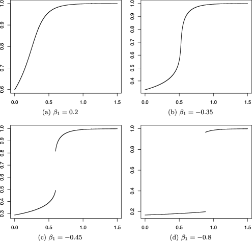
Figure 3: Plot of $u^{*}(\beta_{1},\beta_{2})$ on $y$-axis vs $\beta_{2}$ on $x$-axis for different fixed values of $\beta_{1}$. Part (c) demonstrates a phase transition. Part (d) demonstrates near-degeneracy.

It is likely that $u^{*}(\beta_{1},\beta_{2})$ does not have a closed form expression, other than when $\beta_{2}=0$, in which case

$$u^{*}(\beta_{1},0)=\frac{e^{2\beta_{1}}}{1+e^{2\beta_{1}}}.$$

It is, however, quite easy to numerically approximate $u^{*}(\beta_{1},\beta_{2})$. Figure 3 plots $u^{*}(\beta_{1},\beta_{2})$ versus $\beta_{2}$ for four different fixed values of $\beta_{1}$, namely, $\beta_{1}=0.2$, $-0.35,-0.45$, and $-0.8$. The figures show that $u^{*}$ is a continuous function of $\beta_{2}$ as long as $\beta_{1}$ is not too far down the negative axis.

But for $\beta_{1}$ below a threshold (e.g., when $\beta_{1}=-0.45$), $u^{*}$ shows a single jump discontinuity in $\beta_{2}$, signifying a phase transition. In physical terms, this is a first order phase transition, by the following logic. By Theorem 4.2, our random graph behaves like $G(n,u^{*})$ when $n$ is large. On the other hand, by a standard computation the expect number of triangles is the first derivative of the free energy $\psi_{n}$ with respect to $\beta_{2}$. Therefore in the large $n$ limit, a discontinuity in $u^{*}$ as a function of $\beta_{2}$ signifies a discontinuity in the derivative of the limiting free energy, which is the physical definition of a first order phase transition.

At the point of discontinuity, $\ell(u)$ is maximized at two values of $u$, that is, the set $U$ consists of two points. Lastly, as $\beta_{1}$ goes down the negative axis, the model starts to exhibit “near-degeneracy” in the sense of Handcock handcock (see also park04 ) as seen in the last frame of Figure 3. This means that when $\beta_{1}$ is a large negative number, then as $\beta_{2}$ varies, the model transitions from being a very sparse graph for low values of $\beta_{2}$, to a very dense graph for large values of $\beta_{2}$, completely skipping all intermediate structures. If this sentence is confusing, please see Theorem 5.1 below for a precise statement. This theorem gives a simple mathematical description of this phenomenon and hence the first rigorous proof of the degeneracy observed in exponential graph models. Related results are in Häggstrom and Jonasson hj99 .

Theorem 5.1

Let $G_{n}$ be an exponential random graph with sufficient statistic $T$ defined in (5) and let $\mathbb{P}$ be the probability measure on the underlying probability space on which $G_{n}$ is defined. Fix any $\beta_{1}<0$. Let

$$c_{1}:=\frac{e^{\beta_{1}}}{1+e^{\beta_{1}}},\qquad c_{2}:=1+\frac{1}{2\beta_{1}}.$$

Suppose $|\beta_{1}|$ is so large that $c_{1}<c_{2}$. Let $e(G_{n})$ be the number of edges in $G_{n}$ and let $f(G_{n}):=e(G_{n})/{n\choose 2}$ be the edge density. [Note that $f(G_{n})=\frac{n}{n-1}t(H_{1},G_{n})$, where $H_{1}$ is a single edge.]

Then there exists $q=q(\beta_{1})\in[0,\infty)$ such that if $-\infty<\beta_{2}<q$, then

$$\lim_{n\rightarrow\infty}\mathbb{P}\bigl{(}f(G_{n})>c_{1}\bigr{)}=0,$$

and if $\beta_{2}>q$, then

$$\lim_{n\rightarrow\infty}\mathbb{P}\bigl{(}f(G_{n})<c_{2}\bigr{)}=0.$$

In other words, if $\beta_{1}$ is a large negative number, then $G_{n}$ is either sparse (if $\beta_{2}<q$) or nearly complete (if $\beta_{2}>q$).

The difference in the values of $c_{1}$ and $c_{2}$ can be quite striking even for relatively small values of $\beta_{1}$. For example, $\beta_{1}=-5$ gives $c_{1}\simeq 0.007$ and $c_{2}=0.9$. Significant extensions of Theorem 5.1 have been made in the recent manuscripts aristoffradin , radin1 , radin2 , yin .

6 The symmetric phase, symmetry breaking, and the Euler–Lagrange equations

The purpose of this section is to extend the analysis of the model from Section 4 beyond the case of nonnegative parameters. We begin with a standard approach to solving variational problems.

6.1 Euler–Lagrange equations

We return to the exponential random graph model with sufficient statistic $T$ defined in (16) in terms of the densities of $k$ fixed graphs $H_{1},\ldots,H_{k}$, where $H_{1}$ is a single edge. Theorems 4.1 and 4.2 analyze this model when $\beta_{2},\ldots,\beta_{k}$ are nonnegative. What if they are not? One can still try to derive the Euler–Lagrange equations (or Euler’s equation; see gelfand ) for the related variational problem of maximizing $T({\widetilde{h}})-I({\widetilde{h}})$. The following theorem presents the outcome of this effort.

For a finite simple graph $H$, let $V(H)$ and $E(H)$ denote the sets of vertices and edges of $H$. Given a symmetric measurable function $h\dvtx[0,1]^{2}\to\mathbb{R}$, for each $(r,s)\in E(H)$ and each pair of points $x_{r},x_{s}\in[0,1]$, define

$$\Delta_{H,r,s}h(x_{r},x_{s}):=\int_{[0,1]^{|V(H)\setminus\{r,s\}|}}\mathop{\prod_{(r^{\prime},s^{\prime})\in E(H)}}_{(r^{\prime},s^{\prime})\neq(r,s)}h(x_{r^{\prime}},x_{s^{\prime}})\mathop{\prod_{v\in V(H)}}_{v\neq r,s}\,dx_{v}.$$

For $x,y\in[0,1]$ define

$$\Delta_{H}h(x,y):=\sum_{(r,s)\in E(H)}\Delta_{H,r,s}h(x,y).$$ (20)

For example, when $H$ is a triangle, then $V(H)=\{1,2,3\}$ and

$$\Delta_{H,1,2}h(x,y)=\Delta_{H,1,3}h(x,y)=\Delta_{H,2,3}h(x,y)=\int_{0}^{1}h(x,z)h(y,z)\,dz$$

and therefore $\Delta_{H}h(x,y)=3\int_{0}^{1}h(x,z)h(y,z)\,dz$. When $H$ contains exactly one edge, define $\Delta_{H}h\equiv 1$ for any $h$, by the usual convention that the empty product is $1$. The following theorem gives the Euler–Lagrange equations for the optimizer $h$ of Theorem 3.1 in terms of these $\Delta_{H}h$’s.

Theorem 6.1

Let $T\dvtx\widetilde{\mathcal{W}}\to\mathbb{R}$ be defined as in (16) and the operator $\Delta_{H}$ be defined as in (20). If ${\widetilde{h}}\in\widetilde{\mathcal{W}}$ maximizes $T({\widetilde{h}})-I({\widetilde{h}})$, then any representative element $h\in{\widetilde{h}}$ must satisfy for almost all $(x,y)\in[0,1]^{2}$,

$$h(x,y)=\frac{e^{2\sum_{i=1}^{k}\beta_{i}\Delta_{H_{i}}h(x,y)}}{1+e^{2\sum_{i=1}^{k}\beta_{i}\Delta_{H_{i}}h(x,y)}}.$$

Moreover, any maximizing function must be bounded away from $0$ and $1$.

Unfortunately, these equations may have many solutions and therefore do not uniquely identify the optimizer. The next subsection gives a sufficient condition under which the solution in unique.

6.2 The replica symmetric phase

Borrowing terminology from spinglasses, we define the replica symmetric phase or simply the symmetric phase of a variational problem like maximizing $T(h)-I(h)$ as the set of parameter values for which all the maximizers are constant functions. When the parameters are such that all maximizers are nonconstant functions we say that the parameter vector is in the region of broken replica symmetry, or simply broken symmetry. There may be another situation, where some optimizers are constant while others are nonconstant, although we do not know of such examples. (This third region may be called a region of partial symmetry.)

Statistically, the exponential random graph behaves like an Erdős–Rényi graph in the symmetric region of the parameter space, while such behavior breaks down in the region of broken symmetry. This follows easily from Theorem 3.2.

Theorem 4.2 shows that for the sufficient statistic $T$ defined in (16), each $(\beta_{1},\beta_{2},\ldots,\beta_{k})$ in $\mathbb{R}\times\mathbb{R}_{+}^{k-1}$ falls in the replica symmetric region. Does symmetry hold only when $\beta_{2},\ldots,\beta_{k}$ are nonnegative? The following theorem (proven with the aid of the Euler–Lagrange equations of Theorem 6.1), shows that this is not the case; $(\beta_{1},\ldots,\beta_{k})$ is in the replica symmetric region whenever $|\beta_{2}|,\ldots,|\beta_{k}|$ are small enough. Of course, this does not supersede Theorem 4.2 since it does not cover large positive values of $\beta_{2},\ldots,\beta_{k}$. However, it proves replica symmetry for small negative values of $\beta_{2},\ldots,\beta_{k}$, which is not covered by Theorem 4.2.

Theorem 6.2

Consider the exponential random graph with sufficient statistic $T$ defined in (16). Suppose $\beta_{1},\ldots,\beta_{k}$ are such that

$$\sum_{i=2}^{k}|\beta_{i}|e(H_{i})\bigl{(}e(H_{i})-1\bigr{)}<2,$$

where $e(H_{i})$ is the number of edges in $H_{i}$. Then the conclusions of Theorems 4.1 and 4.2 hold true for this value of the parameter vector $(\beta_{1},\ldots,\beta_{k})$.

6.3 Symmetry breaking

Theorems 4.2 and 6.2 establish various regions of symmetry in the exponential random graph model with sufficient statistic $T$ defined in (16). That leaves the question: is there a region where symmetry breaks? We specialize to the simple case where $k=2$ and $H_{2}$ is a triangle, that is, the example of Section 5. In this case, it turns out that replica symmetry breaks whenever $\beta_{2}$ is less than a sufficiently large negative number depending on $\beta_{1}$.

Theorem 6.3

Consider the exponential random graph with sufficient statistic $T$ defined in (5). Then for any given value of $\beta_{1}$, there is a positive constant $C(\beta_{1})$ sufficiently large so that whenever $\beta_{2}<-C(\beta_{1})$, $T(h)-I(h)$ is not maximized at any constant function. Consequently, if $G_{n}$ is an $n$-vertex exponential random graph with this sufficient statistic, then there exists $\varepsilon>0$ such that

$$\lim_{n\to\infty}\mathbb{P}\bigl{(}\delta_{\Box}(\widetilde{G}_{n},\widetilde{C})>\varepsilon\bigr{)}=1,$$

where $\widetilde{C}$ is the set of constant functions. In other words, $G_{n}$ does not look like an Erdős–Rényi graph in the large $n$ limit.

For interesting recent developments about symmetry breaking in exponential random graph models, see Lubetzky and Zhao lz .

6.4 A completely solvable case

A $j$-star is an undirected graph with one “root” vertex and $j$ other vertices connected to the root vertex, with no edges between any of these $j$ vertices. Let $H_{j}$ be a $j$-star for $j=1,\ldots,k$. Let $T$ be the sufficient statistic

$$T(G)=\sum_{j=1}^{k}\beta_{j}t(H_{j},G).$$ (21)

Theorems 4.1 and 4.2 describe the behavior of this model when $\beta_{2},\ldots,\beta_{k}$ are all nonnegative. The following theorem completely solves this model for all values of $\beta_{2},\ldots,\beta_{k}$. The proof of this theorem was suggested by the anonymous referee, improving upon the version of the result given in an earlier draft.

Theorem 6.4

For the sufficient statistic $T$ defined in (21), the conclusions of Theorems 4.1 and 4.2 hold for any $\beta_{1},\ldots,\beta_{k}\in\mathbb{R}$.

7 Extremal behavior

In the sections above, we have been assuming that $\beta_{2},\ldots,\beta_{k}$ are positive or barely negative. In this section, we investigate what happens when $k=2$ and $\beta_{2}$ is large and negative. The limits are describable but far from Erdős–Rényi. Our work here is inspired by related results of Sukhada Fadvanis who has a different argument (using Turán’s theorem turan ) for the case of triangles.

Suppose $H$ is any finite simple graph containing at least one edge. Let $T$ be the sufficient statistic

$$T(\widetilde{G})=2\beta_{1}\frac{\#\mathrm{edges}\ \mathrm{in}\ G}{n^{2}}+\beta_{2}t(H,G).$$

Let $G_{n}$ be the exponential random graph on $n$ vertices with this sufficient statistic and let $\psi_{n}$ be the associated normalizing constant as defined in (14). Then Theorem 3.1 gives

$$\lim_{n\rightarrow\infty}\psi_{n}=\sup_{h\in\mathcal{W}}\bigl{(}T(h)-I(h)\bigr{)}=:\psi,$$

where $I$ is defined in (15). We also know (by Theorem 3.2) that

$$\delta_{\Box}\bigl{(}\widetilde{G}_{n},\widetilde{F}^{*}\bigr{)}\rightarrow 0\qquad\mbox{in probability as $n\to\infty$,}$$

where $\widetilde{F}^{*}$ is the subset of $\widetilde{\mathcal{W}}$ where $T-I$ is maximized. (Note that ${\widetilde{F}}^{*}$ is a closed set since $T-I$ is an upper semicontinuous map.)

We can compute ${\widetilde{F}}^{*}$ and $\psi$ when $\beta_{2}$ is positive, or negative with small magnitude. We are unable to carry out the explicit computation in the case of large negative $\beta_{2}$, unless $H$ is a convenient object like a $j$-star. However, a qualitative description can still be given by analyzing the behavior of ${\widetilde{F}}^{*}$ and $\psi$ as $\beta_{2}\rightarrow-\infty$. Fixing $\beta_{1}$, we consider these objects as functions of $\beta_{2}$ and write ${\widetilde{F}}^{*}(\beta_{2})$, $\psi(\beta_{2})$ and $T_{\beta_{2}}$ instead of ${\widetilde{F}}^{*}$, $\psi$ and $T$. Recall that the chromatic number of a graph is the minimum number of colors required to color the edges so that no two neighbors get the same color.

Theorem 7.1

Fixing $H$ and $\beta_{1}$, let ${\widetilde{F}}^{*}(\beta_{2})$ and $\psi(\beta_{2})$ be as above. Let $\chi(H)$ be the chromatic number of $H$, and define

$$g(x,y):=\cases{1,&\quad if $\bigl{[}\bigl{(}\chi(H)-1\bigr{)}x\bigr{]}\neq\bigl{[}\bigl{(}\chi(H)-1\bigr{)}y\bigr{]}$,\cr 0,&\quad otherwise,}$$ (22)

where $[x]$ denotes the integer part of a real number $x$. Let $p=e^{2\beta_{1}}/(1+e^{2\beta_{1}})$. Then

$$\lim_{\beta_{2}\to-\infty}\sup_{\widetilde{f}\in{\widetilde{F}}^{*}(\beta_{2})}\delta_{\Box}(\widetilde{f},p\widetilde{g})=0$$

and

$$\lim_{\beta_{2}\to-\infty}\psi(\beta_{2})=\frac{(\chi(H)-2)}{2(\chi(H)-1)}\log\frac{1}{1-p}.$$

Intuitively, the above result means that if $\beta_{2}$ is a large negative number and $n$ is large, then an exponential random graph $G_{n}$ with sufficient statistic $T$ looks roughly like a complete $(\chi(H)-1)$-equipartite graph with $1-p$ fraction of edges randomly deleted, where $p=e^{2\beta_{1}}/(1+e^{2\beta_{1}})$. In particular, if $H$ is bipartite, then $G_{n}$ must be very sparse, since a $1$-equipartite graph has no edges. Figure 4 gives a simulation result for the triangle model with large negative $\beta_{2}$.

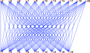
Figure 4: A simulated realization of the exponential random graph model on $20$ nodes with edges and triangles as sufficient statistics, where $\beta_{1}=120$ and $\beta_{2}=-400$. (Picture by Sukhada Fadnavis. Gibbs sampling used in simulations. We are unsure about the convergence of the MCMC algorithm used to generate these grapgs, but the structure of the simulated graphs match the predictions of Theorem 7.1.)

Theorem 7.1 is closely related to the Erdős–Stone theorem erdosstone from extremal graph theory (or equivalently, Turán’s theorem in the case of triangles as in the work of Fadnavis). Indeed, it may be possible to prove some parts of our theorem using the Erdős–Stone theorem, but we prefer a bare-hands argument given in Section 8. Due to this connection with extremal graph theory, we refer to behavior of the graph in the “large negative $\beta_{2}$” domain as extremal behavior.

8 Proofs

Proof of Theorem 3.1 For each Borel set $\widetilde{A}\subseteq\widetilde{\mathcal{W}}$ and each $n$, define

$$\widetilde{A}_{n}:=\{{\widetilde{h}}\in\widetilde{A}\dvtx{\widetilde{h}}=\widetilde{G}\mbox{ for some }G\in\mathcal{G}_{n}\}.$$

Let $\mathbb{P}_{n,p}$ be the Erdős–Rényi measure defined in Section 2.3. Note that $\widetilde{A}_{n}$ is a finite set and

$$|\widetilde{A}_{n}|=2^{n(n-1)/2}\mathbb{P}_{n,1/2}(\widetilde{A}_{n})=2^{n(n-1)/2}\mathbb{P}_{n,1/2}(\widetilde{A}).$$

Thus, if ${\widetilde{F}}$ is a closed subset of $\widetilde{\mathcal{W}}$ then by Theorem 2.1

$$\limsup_{n\to\infty}\frac{\log|{\widetilde{F}}_{n}|}{n^{2}} \leq \frac{\log 2}{2}-\inf_{{\widetilde{h}}\in{\widetilde{F}}}I_{1/2}({\widetilde{h}})$$

$$= -\inf_{{\widetilde{h}}\in{\widetilde{F}}}I({\widetilde{h}}).$$

Similarly if $\widetilde{U}$ is an open subset of $\widetilde{\mathcal{W}}$,

$$\liminf_{n\to\infty}\frac{\log|\widetilde{U}_{n}|}{n^{2}}\geq-\inf_{{\widetilde{h}}\in\widetilde{U}}I({\widetilde{h}}).$$ (24)

Fix $\varepsilon>0$. Since $T$ is a bounded function, there is a finite set $R$ such that the intervals $\{(a,a+\varepsilon)\dvtx a\in R\}$ cover the range of $T$. For each $a\in R$, let ${\widetilde{F}}^{a}:=T^{-1}([a,a+\varepsilon])$. By the continuity of $T$, each ${\widetilde{F}}^{a}$ is closed. Now,

$$e^{n^{2}\psi_{n}}\leq\sum_{a\in R}e^{n^{2}(a+\varepsilon)}\bigl{|}{\widetilde{F}}^{a}_{n}\bigr{|}\leq|R|\sup_{a\in R}e^{n^{2}(a+\varepsilon)}\bigl{|}{\widetilde{F}}^{a}_{n}\bigr{|}.$$

By (8), this shows that

$$\limsup_{n\to\infty}\psi_{n}\leq\sup_{a\in R}\Bigl{(}a+\varepsilon-\inf_{{\widetilde{h}}\in{\widetilde{F}}^{a}}I({\widetilde{h}})\Bigr{)}.$$

Each ${\widetilde{h}}\in{\widetilde{F}}^{a}$ satisfies $T({\widetilde{h}})\geq a$. Consequently,

$$\sup_{{\widetilde{h}}\in{\widetilde{F}}^{a}}\bigl{(}T({\widetilde{h}})-I({\widetilde{h}})\bigr{)}\geq\sup_{{\widetilde{h}}\in{\widetilde{F}}^{a}}\bigl{(}a-I({\widetilde{h}})\bigr{)}=a-\inf_{{\widetilde{h}}\in{\widetilde{F}}^{a}}I({\widetilde{h}}).$$

Substituting this in the earlier display gives

$$\limsup_{n\to\infty}\psi_{n} \leq \varepsilon+\sup_{a\in R}\sup_{{\widetilde{h}}\in{\widetilde{F}}^{a}}\bigl{(}T({\widetilde{h}})-I({\widetilde{h}})\bigr{)}$$

$$= \varepsilon+\sup_{{\widetilde{h}}\in\widetilde{\mathcal{W}}}\bigl{(}T({\widetilde{h}})-I({\widetilde{h}})\bigr{)}.$$

For each $a\in R$, let ${\widetilde{U}}^{a}:=T^{-1}((a,a+\varepsilon))$. By the continuity of $T$, ${\widetilde{U}}^{a}$ is an open set. Note that

$$e^{n^{2}\psi_{n}}\geq\sup_{a\in R}e^{n^{2}a}\bigl{|}{\widetilde{U}}^{a}_{n}\bigr{|}.$$

Therefore by (24), for each $a\in R$

$$\liminf_{n\to\infty}\psi_{n}\geq a-\inf_{{\widetilde{h}}\in{\widetilde{U}}^{a}}I({\widetilde{h}}).$$

Each ${\widetilde{h}}\in{\widetilde{U}}^{a}$ satisfies $T({\widetilde{h}})<a+\varepsilon$. Therefore,

$$\sup_{{\widetilde{h}}\in{\widetilde{U}}^{a}}\bigl{(}T({\widetilde{h}})-I({\widetilde{h}})\bigr{)}\leq\sup_{{\widetilde{h}}\in{\widetilde{U}}^{a}}\bigl{(}a+\varepsilon-I({\widetilde{h}})\bigr{)}=a+\varepsilon-\inf_{{\widetilde{h}}\in{\widetilde{U}}^{a}}I({\widetilde{h}}).$$

Together with the previous display, this shows that

$$\liminf_{n\to\infty}\psi_{n} \geq -\varepsilon+\sup_{a\in R}\sup_{{\widetilde{h}}\in{\widetilde{U}}^{a}}\bigl{(}T({\widetilde{h}})-I({\widetilde{h}})\bigr{)}$$

$$= -\varepsilon+\sup_{{\widetilde{h}}\in\widetilde{\mathcal{W}}}\bigl{(}T({\widetilde{h}})-I({\widetilde{h}})\bigr{)}.$$

Since $\varepsilon$ is arbitrary in (8) and (8), this completes the proof.

Proof of Theorem 3.2 Take any $\eta>0$. Let

$$\widetilde{A}:=\bigl{\{}{\widetilde{h}}\dvtx\delta_{\Box}\bigl{(}{\widetilde{h}},{\widetilde{F}}^{*}\bigr{)}\geq\eta\bigr{\}}.$$

It is easy to see that $\widetilde{A}$ is a closed set. By compactness of $\widetilde{\mathcal{W}}$ and ${\widetilde{F}}^{*}$, and upper semi-continuity of $T-I$, it follows that

$$2\gamma:=\sup_{{\widetilde{h}}\in\widetilde{\mathcal{W}}}\bigl{(}T({\widetilde{h}})-I({\widetilde{h}})\bigr{)}-\sup_{{\widetilde{h}}\in\widetilde{A}}\bigl{(}T({\widetilde{h}})-I({\widetilde{h}})\bigr{)}>0.$$

Choose $\varepsilon=\gamma$ and define ${\widetilde{F}}^{a}$ and $R$ as in the proof of Theorem 3.1. Let $\widetilde{A}{}^{a}:=\widetilde{A}\cap{\widetilde{F}}^{a}$. Then

$$\mathbb{P}(G_{n}\in\widetilde{A})\leq e^{-n^{2}\psi_{n}}\sum_{a\in R}e^{n^{2}(a+\varepsilon)}\bigl{|}\widetilde{A}{}^{a}_{n}\bigr{|}\leq e^{-n^{2}\psi_{n}}|R|\sup_{a\in R}e^{n^{2}(a+\varepsilon)}\bigl{|}\widetilde{A}{}^{a}_{n}\bigr{|}.$$

While bounding the last term above, it can be assumed without loss of generality that $\widetilde{A}{}^{a}$ is nonempty for each $a\in R$, for the other $a$’s can be dropped without upsetting the bound. By (8) and Theorem 3.1 (noting that $\widetilde{A}{}^{a}$ is compact), the above display gives

$$\limsup_{n\to\infty}\frac{\log\mathbb{P}(G_{n}\in\widetilde{A})}{n^{2}}\leq\sup_{a\in R}\Bigl{(}a+\varepsilon-\inf_{{\widetilde{h}}\in\widetilde{A}{}^{a}}I({\widetilde{h}})\Bigr{)}-\sup_{{\widetilde{h}}\in\widetilde{\mathcal{W}}}\bigl{(}T({\widetilde{h}})-I({\widetilde{h}})\bigr{)}.$$

Each ${\widetilde{h}}\in\widetilde{A}{}^{a}$ satisfies $T({\widetilde{h}})\geq a$. Consequently,

$$\sup_{{\widetilde{h}}\in\widetilde{A}{}^{a}}\bigl{(}T({\widetilde{h}})-I({\widetilde{h}})\bigr{)}\geq\sup_{{\widetilde{h}}\in\widetilde{A}{}^{a}}\bigl{(}a-I({\widetilde{h}})\bigr{)}=a-\inf_{{\widetilde{h}}\in\widetilde{A}{}^{a}}I({\widetilde{h}}).$$

Substituting this in the earlier display gives

$$\limsup_{n\to\infty}\frac{\log\mathbb{P}(G_{n}\in\widetilde{A})}{n^{2}} \leq \varepsilon+\sup_{a\in R}\sup_{{\widetilde{h}}\in\widetilde{A}{}^{a}}\bigl{(}T({\widetilde{h}})-I({\widetilde{h}})\bigr{)}-\sup_{{\widetilde{h}}\in\widetilde{\mathcal{W}}}\bigl{(}T({\widetilde{h}})-I({\widetilde{h}})\bigr{)}$$

$$= \varepsilon+\sup_{{\widetilde{h}}\in\widetilde{A}}\bigl{(}T({\widetilde{h}})-I({\widetilde{h}})\bigr{)}-\sup_{{\widetilde{h}}\in\widetilde{\mathcal{W}}}\bigl{(}T({\widetilde{h}})-I({\widetilde{h}})\bigr{)}.$$

$$= \varepsilon-2\gamma=-\gamma.$$

This completes the proof.

Proof of Theorem 4.1 By Theorem 3.1,

$$\lim_{n\to\infty}\psi_{n}=\sup_{h\in\mathcal{W}}\bigl{(}T(h)-I(h)\bigr{)}.$$ (27)

By Hölder’s inequality,

$$t(H_{i},h)\leq\int\!\!\int_{[0,1]^{2}}h(x,y)^{e(H_{i})}\,dx\,dy.$$

Thus, by the nonnegativity of $\beta_{2},\ldots,\beta_{k}$,

$$T(h) \leq \beta_{1}t(H_{1},h)+\sum_{i=2}^{k}\beta_{i}\int\!\!\int_{[0,1]^{2}}h(x,y)^{e(H_{i})}\,dx\,dy$$

$$= \int\!\!\int_{[0,1]^{2}}\sum_{i=1}^{k}\beta_{i}h(x,y)^{e(H_{i})}\,dx\,dy.$$

On the other hand, the inequality in the above display becomes an equality if $h$ is a constant function. Therefore, if $u$ is a point in $[0,1]$ that maximizes

$$\sum_{i=1}^{k}\beta_{i}u^{e(H_{i})}-I(u),$$

then the constant function $h(x,y)\equiv u$ solves the variational problem (27). To see that constant functions are the only solutions, assume that there is at least one $i$ such that the graph $H_{i}$ has at least one vertex with two or more neighbors. The above steps show that if $h$ is a maximizer, then for each $i$,

$$t(H_{i},h)=\int\!\!\int_{[0,1]^{2}}h(x,y)^{e(H_{i})}\,dx\,dy.$$ (28)

In other words, equality holds in Hölder’s inequality. Suppose that $H_{i}$ has vertex set $\{1,2,\ldots,k\}$ and vertices $2$ and $3$ are both neighbors of $1$ in $H_{i}$. Recall that

$$t(H_{i},h)=\int_{[0,1]^{k}}\prod_{\{j,l\}\in E(H_{i})}h(x_{j},x_{l})\,dx_{1}\cdots dx_{k}.$$

In particular, the integrand contains the product $h(x_{1},x_{2})h(x_{1},x_{3})$. From this and the criterion for equality in Hölder’s inequality, it follows that $h(x_{1},x_{2})=h(x_{1},x_{3})$ for almost every $(x_{1},x_{2},x_{3})$. Using the symmetry of $h$ one can now easily conclude that $h$ is almost everywhere a constant function.

If the condition does not hold, then each $H_{i}$ is a union of vertex-disjoint edges. Assume that some $H_{i}$ has more than one edge. Then again by (28) it follows that $h$ must be a constant function.

Finally, if each $H_{i}$ is just a single edge, then the maximization problem (27) can be explicitly solved and the solutions are all constant functions.

Proof of Theorem 4.2 The assertions about graph limits in this theorem are direct consequences of Theorems 3.2 and 4.1. Since $\sum_{i=1}^{k}\beta_{i}u^{e(H_{i})}$ is a polynomial function of $u$ and $I(u)$ is sufficiently well-behaved, showing that $U$ is a finite set is a simple analytical exercise.

Proof of Theorem 5.1 Fix $\beta_{1}<0$ such that $c_{1}<c_{2}$. As a preliminary step, let us prove that for any $\beta_{2}>0$,

$$\lim_{n\to\infty}\mathbb{P}\bigl{(}f(G_{n})\in(c_{1},c_{2})\bigr{)}=0.$$ (29)

Fix $\beta_{2}>0$. Let $u$ be any maximizer of $\ell$. Then by Theorem 4.2, it suffices to prove that either $u<e^{\beta_{1}}/(1+e^{\beta_{1}})$ or $u>1+1/2\beta_{1}$. This is proved as follows. Define a function $g\dvtx[0,1]\to\mathbb{R}$ as

$$g(v):=\ell\bigl{(}v^{1/3}\bigr{)}.$$

Then $\ell$ is maximized at $u$ if and only if $g$ is maximized at $u^{3}$. Since $\ell$ is a bounded continuous function and $\ell^{\prime}(0)=\infty$, $\ell^{\prime}(1)=-\infty$, $\ell$ cannot be maximized at $0$ or $1$. Therefore, the same is true for $g$. Let $v$ be a point in $(0,1)$ at which $g$ is maximized. Then $g^{\prime\prime}(v)\leq 0$. A simple computation shows that

$$g^{\prime\prime}(v)=\frac{1}{9v^{5/3}}\biggl{(}-2\beta_{1}+\log\frac{v^{1/3}}{1-v^{1/3}}-\frac{1}{2(1-v^{1/3})}\biggr{)}.$$

Thus, $g^{\prime\prime}(v)\leq 0$ only if

$$\log\frac{v^{1/3}}{1-v^{1/3}}\leq\beta_{1}\quad\mbox{or}\quad-\frac{1}{2(1-v^{1/3})}\leq\beta_{1}.$$

This shows that a maximizer $u$ of $\ell$ must satisfy $u\leq c_{1}$ or $u\geq c_{2}$. Now, if $u=c_{1}$, then $u<c_{2}$, and therefore the above computations show that $g^{\prime\prime}(v)>0$, where $v=u^{3}$. Similarly, if $u=c_{2}$ then $u>c_{1}$ and again $g^{\prime\prime}(v)>0$. Thus, we have proved that $u<c_{1}$ or $u>c_{2}$. By Theorem 3.2, this completes the proof of (29) when $\beta_{2}>0$.

Now notice that as $\beta_{2}\rightarrow\infty$, $\sup_{u\leq a}\ell(u)\sim\beta_{2}a^{3}$ for any fixed $a\leq 1$. This shows that as $\beta_{2}\rightarrow\infty$, any maximizer of $\ell$ must eventually be larger than $1+1/2\beta_{1}$. Therefore, for sufficiently large $\beta_{2}$,

$$\lim_{n\rightarrow\infty}\mathbb{P}\bigl{(}f(G_{n})<c_{2}\bigr{)}=0.$$ (30)

Next consider the case $\beta_{2}\leq 0$. Let ${\widetilde{F}}^{*}$ be the set of maximizers of $T({\widetilde{h}})-I({\widetilde{h}})$. Take any ${\widetilde{h}}\in{\widetilde{F}}^{*}$ and let $h$ be a representative element of ${\widetilde{h}}$. Let $p=e^{2\beta_{1}}/(1+e^{2\beta_{1}})$. An easy verification shows that

$$T(h)-I(h)=\beta_{2}t(H_{2},h)-I_{p}(h)-\tfrac 12\log(1-p),$$

where $I_{p}(h)$ is defined as in (11). Define a new function

$$h_{1}(x,y):=\min\bigl{\{}h(x,y),p\bigr{\}}.$$

Since the function $I_{p}$ defined in (10) is minimized at $p$, it follows that for all $x,y\in[0,1]$, $I_{p}(h_{1}(x,y))\leq I_{p}(h(x,y))$. Consequently, $I_{p}(h_{1})\leq I_{p}(h)$. Again, since $\beta_{2}\leq 0$ and $h_{1}\leq h$ everywhere, $\beta_{2}t(H_{2},h_{1})\geq\beta_{2}t(H_{2},h)$. Combining these observations, we see that $T(h_{1})-I(h_{1})\geq T(h)-I(h)$. Since $h$ maximizes $T-I$ it follows that equality must hold at every step in the above deductions, from which it is easy to conclude that $h=h_{1}$ a.e. In other words, $h(x,y)\leq p$ a.e. This is true for every ${\widetilde{h}}\in{\widetilde{F}}^{*}$. Since $p<c_{1}$, the above deduction coupled with Theorem 3.2 proves that when $\beta_{2}\leq 0$,

$$\lim_{n\rightarrow\infty}\mathbb{P}\bigl{(}f(G_{n})>c_{1}\bigr{)}=0.$$ (31)

Recalling that $\beta_{1}$ is fixed, define

$$a_{n}(\beta_{2}):=\mathbb{P}\bigl{(}f(G_{n})>c_{1}\bigr{)},\qquad b_{n}(\beta_{2}):=\mathbb{P}\bigl{(}f(G_{n})<c_{2}\bigr{)}.$$

Let $A_{n}$ and $B_{n}$ denote the events in brackets in the above display. A simple computation shows that

$$a_{n}^{\prime}(\beta_{2})=\frac{6}{n}\operatorname{Cov}\bigl{(}1_{A_{n}},\Delta(G_{n})\bigr{)}\quad\mbox{and}\quad b_{n}^{\prime}(\beta_{2})=\frac{6}{n}\operatorname{Cov}\bigl{(}1_{B_{n}},\Delta(G_{n})\bigr{)},$$

where $\Delta(G_{n})$ is the number of triangles in $G_{n}$. As noted at the end of Section 4, the exponential random graph model with $\beta_{2}\geq 0$ satisfies the FKG criterion fkg71 . Therefore, the above identities show that on the nonnegative axis, $a_{n}$ is a nondecreasing function and $b_{n}$ is a nonincreasing function.

Let $q_{1}:=\sup\{x\in\mathbb{R}\dvtx\lim_{n\rightarrow\infty}a_{n}(x)=0\}$. By equation (30), $q_{1}<\infty$ and by equation (31) $q_{1}\geq 0$. Similarly, if $q_{2}:=\inf\{x\in\mathbb{R}\dvtx\lim_{n\rightarrow\infty}b_{n}(x)=0\}$, then $0\leq q_{2}<\infty$. Also, clearly, $q_{1}\leq q_{2}$ since $a_{n}+b_{n}\geq 1$ everywhere. We claim that $q_{1}=q_{2}$. This would complete the proof by the monotonicity of $a_{n}$ and $b_{n}$.

To prove that $q_{1}=q_{2}$, suppose not. Then $q_{1}<q_{2}$. Then for any $\beta_{2}\in(q_{1},q_{2})$, $\limsup a_{n}(\beta_{2})>0$ and $\limsup b_{n}(\beta_{2})>0$. Now,

$$0\leq a_{n}(\beta_{2})+b_{n}(\beta_{2})-1=\mathbb{P}\bigl{(}f(G_{n})\in(c_{1},c_{2})\bigr{)}.$$

Therefore by (29),

$$\lim_{n\rightarrow\infty}\bigl{(}a_{n}(\beta_{2})+b_{n}(\beta_{2})-1\bigr{)}=0.$$

Thus, for any $\beta_{2}\in(q_{1},q_{2})$, $\limsup(1-b_{n}(\beta_{2}))>0$. By Theorem 4.2, this implies that the function $\ell$ has a maximum in $[c_{2},1]$. Similarly, for any $\beta_{2}\in(q_{1},q_{2})$, $\limsup(1-a_{n}(\beta_{2}))>0$ and therefore the function $\ell$ has a maximum in $[0,c_{1}]$. Now fix $q_{1}<\beta_{2}<\widetilde{\beta}_{2}<q_{2}$, and let $\ell$ and $\widetilde{\ell}$ denote the two $\ell$-functions corresponding to $\beta_{2}$ and $\widetilde{\beta}_{2}$, respectively. That is,

$$\ell(u)=\beta_{1}u+\beta_{2}u^{3}-I(u),\qquad\widetilde{\ell}(u)=\beta_{1}u+\widetilde{\beta}_{2}u^{3}-I(u).$$

By the above argument, $\ell$ attains its maximum at some point $u_{1}\in[0,c_{1}]$ and at some point $u_{2}\in[c_{2},1]$. (There may be other maxima, but that is irrelevant for us.) Note that

$$\max_{u\leq c_{1}}\widetilde{\ell}(u)=\max_{u\leq c_{1}}\bigl{(}\ell(u)+(\widetilde{\beta}_{2}-\beta_{2})u^{3}\bigr{)}\leq\ell(u_{1})+(\widetilde{\beta}_{2}-\beta_{2})c_{1}^{3}.$$

On the other hand

$$\max_{u\geq c_{2}}\widetilde{\ell}(u)\geq\widetilde{\ell}(u_{2})=\ell(u_{2})+(\widetilde{\beta}_{2}-\beta_{2})u_{2}^{3}\geq\ell(u_{2})+(\widetilde{\beta}_{2}-\beta_{2})c_{2}^{3}.$$

Since $\ell(u_{1})=\ell(u_{2})$, $\widetilde{\beta}_{2}>\beta_{2}$ and $c_{2}>c_{1}$, this shows that

$$\max_{u\leq c_{1}}\widetilde{\ell}(u)<\max_{u\geq c_{2}}\widetilde{\ell}(u),$$

contradicting our previous deduction that $\widetilde{\ell}$ has maxima in both $[0,c_{1}]$ and $[c_{2},1]$. This proves that $q_{1}=q_{2}$.

Proof of Theorem 6.1 Let $g$ be a symmetric bounded measurable function from $[0,1]$ into $\mathbb{R}$. For each $u\in\mathbb{R}$, let

$$h_{u}(x,y):=h(x,y)+ug(x,y).$$

Then $h_{u}$ is a symmetric bounded measurable function from $[0,1]$ into $\mathbb{R}$. First, suppose that $h$ is bounded away from $0$ and $1$. Then $h_{u}\in\mathcal{W}$ for every $u$ sufficiently small in magnitude. Since $h$ maximizes $T(h)-I(h)$ among all elements of $\mathcal{W}$, therefore under the above assumption, for all $u$ sufficiently close to zero,

$$T(h_{u})-I(h_{u})\leq T(h)-I(h).$$

In particular,

$$\frac{d}{du}\bigl{(}T(h_{u})-I(h_{u})\bigr{)}\bigg{|}_{u=0}=0.$$ (32)

It is easy to check that $T(h_{u})-I(h_{u})$ is differentiable in $u$ for any $h$ and $g$. In particular, the derivative is given by

$$\frac{d}{du}\bigl{(}T(h_{u})-I(h_{u})\bigr{)}=\sum_{i=1}^{k}\beta_{i}\,\frac{d}{du}t(H_{i},h_{u})-\frac{d}{du}I(h_{u}).$$

Now,

$$\frac{d}{du}I(h_{u}) = \int\!\!\int\frac{d}{du}I\bigl{(}h(x,y)+ug(x,y)\bigr{)}\,dy\,dx$$

$$= \frac{1}{2}\int\!\!\int g(x,y)\log\frac{h_{u}(x,y)}{1-h_{u}(x,y)}\,dy\,dx.$$

Consequently,

$$\frac{d}{du}I(h_{u})\bigg{|}_{u=0}=\frac{1}{2}\int\!\!\int g(x,y)\log\frac{h(x,y)}{1-h(x,y)}\,dy\,dx.$$

Next, note that

$$\frac{d}{du}t(H_{i},h_{u})$$

$$\qquad=\int_{[0,1]^{V(H)}}\sum_{(r,s)\in E(H_{i})}g(x_{r},x_{s})\mathop{\prod_{(r^{\prime},s^{\prime})\in E(H_{i})}}_{(r^{\prime},s^{\prime})\neq(r,s)}h_{u}(x_{r^{\prime}},x_{s^{\prime}})\prod_{v\in V(H)}\,dx_{v}$$

$$\qquad=\int\!\!\int g(x,y)\Delta_{H_{i}}h_{u}(x,y)\,dy\,dx.$$

Combining the above computations and (32), we see that for any symmetric bounded measurable $g\dvtx[0,1]\to\mathbb{R}$,

$$\int\!\!\int g(x,y)\Biggl{(}\sum_{i=1}^{k}\beta_{i}\Delta_{H_{i}}h(x,y)-\frac{1}{2}\log\frac{h(x,y)}{1-h(x,y)}\Biggr{)}\,dy\,dx=0.$$

Taking $g(x,y)$ equal to the function within the brackets (which is bounded since $h$ is assumed to be bounded away from $0$ and $1$), the conclusion of the theorem follows.

Now note that the theorem was proved under the assumption that $h$ is bounded away from $0$ and $1$. We claim that this is true for any $h$ that maximizes $T(h)-I(h)$. To prove this claim, take any such $h$. Fix $p\in(0,1)$. For each $u\in[0,1]$, let

$$h_{p,u}(x,y):=h(x,y)+u\bigl{(}p-h(x,y)\bigr{)}_{+}.$$

In other words, $h_{p,u}$ is simply $h_{u}$ with $g=(p-h)_{+}$. Then certainly, $h_{p,u}$ is a symmetric bounded measurable function from $[0,1]^{2}$ into $[0,1]$. Note that

$$\frac{d}{du}h_{p,u}(x,y)=\bigl{(}p-h(x,y)\bigr{)}_{+}.$$

Using this, an easy computation as above shows that

$$\frac{d}{du}\bigl{(}T(h_{p,u})-I(h_{p,u})\bigr{)}\bigg{|}_{u=0}$$

$$\qquad=\int\!\!\int\Biggl{(}\sum_{i=1}^{k}\beta_{i}\Delta_{H_{i}}h(x,y)-\frac{1}{2}\log\frac{h(x,y)}{1-h(x,y)}\Biggr{)}\bigl{(}p-h(x,y)\bigr{)}_{+}\,dy\,dx$$

$$\qquad\geq\int\!\!\int\biggl{(}-C-\frac{1}{2}\log\frac{h(x,y)}{1-h(x,y)}\biggr{)}\bigl{(}p-h(x,y)\bigr{)}_{+}\,dy\,dx,$$

where $C$ is a positive constant depending only on $\beta_{1},\ldots,\beta_{k}$ and $H_{1},\ldots,H_{k}$ (and not on $p$ or $h$). When $h(x,y)=0$, the integrand is interpreted as $\infty$, and when $h(x,y)=1$, the integrand is interpreted as $0$.

Now, if $p$ is so small that

$$-C-\frac{1}{2}\log\frac{p}{1-p}>0,$$

then the previous display proves that the derivative of $T(h_{p,u})-I(h_{p,u})$ with respect to $u$ is strictly positive at $u=0$ if $h<p$ on a set of positive Lebesgue measure. Hence, $h$ cannot be a maximizer of $T-I$ unless $h\geq p$ almost everywhere. This proves that any maximizer of $T-I$ must be bounded away from zero. A similar argument with $g=-(h-p)_{+}$ shows that it must be bounded away from $1$, and hence completes the proof of the theorem.

Proof of Theorem 6.2 It suffices to prove that the maximizer of $T(h)-I(h)$ as $h$ varies over $\mathcal{W}$ is unique. This is because: if $h$ is a maximizer, then so is $h_{\sigma}(x,y):=h(\sigma x,\sigma y)$ for any measure preserving bijection $\sigma\dvtx[0,1]\to[0,1]$. The only functions that are invariant under such transforms are constant functions.

Let $\Delta_{H}$ be the operator defined in Section 6.1. Let $\|\cdot\|_{\infty}$ denote the $L^{\infty}$ norm on $\mathcal{W}$ (i.e., the essential supremum of the absolute value). Let $h$ and $g$ be two maximizers of $T-I$. For any finite simple graph $H$, a simple computation shows that

$$\|\Delta_{H}h-\Delta_{H}g\|_{\infty} \leq \sum_{(r,s)\in E(H)}\|\Delta_{H,r,s}h-\Delta_{H,r,s}g\|_{\infty}$$

$$\leq e(H)\bigl{(}e(H)-1\bigr{)}\|h-g\|_{\infty}.$$

Using the above inequality, Theorem 6.1 and the inequality

$$\biggl{|}\frac{e^{x}}{1+e^{x}}-\frac{e^{y}}{1+e^{y}}\biggr{|}\leq\frac{|x-y|}{4}$$

(easily proved by the mean value theorem) it follows that for almost all $x,y$,

$$\bigl{|}h(x,y)-g(x,y)\bigr{|} = \biggl{|}\frac{e^{2\sum_{i=1}^{k}\beta_{i}\Delta_{H_{i}}h(x,y)}}{1+e^{2\sum_{i=1}^{k}\beta_{i}\Delta_{H_{i}}h(x,y)}}-\frac{e^{2\sum_{i=1}^{k}\beta_{i}\Delta_{H_{i}}g(x,y)}}{1+e^{2\sum_{i=1}^{k}\beta_{i}\Delta_{H_{i}}g(x,y)}}\biggr{|}$$

$$\leq \frac{1}{2}\sum_{i=1}^{k}|\beta_{i}|\|\Delta_{H_{i}}h-\Delta_{H_{i}}g\|_{\infty}$$

$$\leq \frac{1}{2}\|h-g\|_{\infty}\sum_{i=1}^{k}|\beta_{i}|e(H_{i})\bigl{(}e(H_{i})-1\bigr{)}.$$

If the coefficient of $\|h-g\|_{\infty}$ in the last expression is strictly less than $1$, it follows that $h$ must be equal to $g$ a.e.

Proof of Theorem 6.3 Fix $\beta_{1}$. Let $p=e^{2\beta_{1}}/(1+e^{2\beta_{1}})$ and $\gamma:=-\beta_{2}$, so that for any $h\in\mathcal{W}$,

$$T(h)-I(h)=-\gamma t(H_{2},h)-I_{p}(h)-\tfrac{1}{2}\log(1-p).$$

Assume without loss of generality that $\beta_{2}<0$. Suppose $u$ is a constant such that the function $h(x,y)\equiv u$ maximizes $T(h)-I(h)$, that is, minimizes $\gamma t(H_{2},h)+I_{p}(h)$. Note that

$$\gamma t(H_{2},h)+I_{p}(h)=\gamma u^{3}+I_{p}(u).$$

Clearly, the definition of $u$ implies that $\gamma u^{3}+I_{p}(u)\leq\gamma x^{3}+I_{p}(x)$ for all $x\in[0,1]$. This implies that $u$ must be in $(0,1)$, because the derivative of $x\mapsto\gamma x^{3}+I_{p}(x)$ is $-\infty$ at $0$ and $\infty$ at $1$. Thus,

$$0=\frac{d}{dx}\bigl{(}\gamma x^{3}+I_{p}(x)\bigr{)}\bigg{|}_{x=u}=3\gamma u^{2}+\frac{1}{2}\log\frac{u}{1-u}-\frac{1}{2}\log\frac{p}{1-p},$$

which shows that $u\leq c(\gamma)$, where $c(\gamma)$ is a function of $\gamma$ such that

$$\lim_{\gamma\to\infty}c(\gamma)=0.$$

This shows that

$$\lim_{\gamma\to\infty}\min_{0\leq x\leq 1}\bigl{(}\gamma x^{3}+I_{p}(x)\bigr{)}=I_{p}(0)=\frac{1}{2}\log\frac{1}{1-p}.$$ (33)

Next, let $g$ be the function

$$g(x,y):=\cases{0,&\quad if $x,y$ on same side of $1/2$,\cr p,&\quad if not.}$$

Clearly, for almost all $(x,y,z)$, $g(x,y)g(y,z)g(z,x)=0$. Thus, $t(H_{2},g)=0$. A simple computation shows that

$$I_{p}(g)=\frac{1}{4}\log\frac{1}{1-p}.$$

Thus, $\gamma t(H_{2},g)+I_{p}(g)=\frac{1}{4}\log\frac{1}{1-p}$. This shows that if $\gamma$ is large enough (depending on $p$ and hence $\beta_{1}$), then $T-I$ cannot be maximized at a constant function. The rest of the conclusion follows easily from Theorem 3.2 and the compactness of $\widetilde{\mathcal{W}}$.

Proof of Theorem 6.4 Take any $h\in\mathcal{W}$. Note that

$$t(H_{j},h) = \int_{[0,1]^{j}}h(x_{1},x_{2})h(x_{1},x_{3})\cdots h(x_{1},x_{j})\,dx_{1}\cdots dx_{j}$$

$$= \int_{0}^{1}M(x)^{j}\,dx,$$

where

$$M(x)=\int_{0}^{1}h(x,y)\,dy.$$

Since $I$ is a convex function,

$$\int_{0}^{1}I\bigl{(}h(x,y)\bigr{)}\,dy\geq I\bigl{(}M(x)\bigr{)}$$

with equality if and only if $h(x,y)$ is the same for almost all $y$. Thus, putting

$$P(u):=\sum_{j=1}^{k}\beta_{j}u^{j},$$

we get

$$T(h)-I(h)=\int_{0}^{1}P\bigl{(}M(x)\bigr{)}\,dx-I(h)\leq\int_{0}^{1}\bigl{(}P\bigl{(}M(x)\bigr{)}-I\bigl{(}M(x)\bigr{)}\bigr{)}\,dx$$

with equality if and only if for almost all $x$, (a) $h(x,y)$ is constant as a function of $y$, and (b) $M(x)$ equals a value $u^{*}$ that maximizes $P(u)-I(u)$. By the symmetry of $h$, the condition (a) implies that $h$ is constant almost everywhere. The condition (b) gives the set of possible values of this constant. The rest follows as in the proofs of Theorems 4.1 and 4.2.

Lemma 8.1

Let $r$ be any integer $\geq\chi(H)$. Let $K_{r}$ be the complete graph on $r$ vertices. Then for any symmetric measurable $h\dvtx[0,1]^{2}\rightarrow\{0,1\}$, if $t(K_{r},h)>0$ then $t(H,h)>0$.

Let $h_{n}(x,y)$ be the average value of $h$ in the dyadic square of width $2^{-n}$ containing the point $(x,y)$. A standard martingale argument implies that the sequence of functions $\{h_{n}\}_{n\geq 1}$ converges to $h$ almost everywhere. For any positive integer $u$, let $K_{r}^{u}$ denote the complete $r$-partite graph on $ru$ vertices, where each partition consists of $u$ vertices (so that $K_{r}^{1}=K_{r}$). Since $r\geq\chi(H)$, it is easy to see that there exists $u$ so large that $H$ is a subgraph of $K_{r}^{u}$ [i.e., $V(H)\subseteq V(K^{u}_{r})$ and $E(H)\subseteq E(K^{u}_{r})$]. Fix such a $u$.

By the almost everywhere convergence of $h_{n}$ to $h$ and the assumption that $t(K_{r},h)>0$, there is a set of $r$ distinct points $x_{1},\ldots,x_{r}\in[0,1]$ that do not lie on the boundary of any dyadic interval, such that $h(x_{i},x_{j})>0$ and $\lim_{n\rightarrow\infty}h_{n}(x_{i},x_{j})=h(x_{i},x_{j})$ for each $1\leq i\neq j\leq r$. Since $h$ is $\{0,1\}$-valued, $h(x_{i},x_{j})=1$ for each $i\neq j$. Choose $n$ so large that for each $i\neq j$,

$$h_{n}(x_{i},x_{j})\geq 1-\varepsilon,$$

where $\varepsilon=1/2r^{2}u^{2}$. Let $(X^{s}_{i})_{1\leq i\leq r,1\leq s\leq u}$ be independent random variables, where $X^{s}_{i}$ is uniformly distributed in the dyadic interval of width $2^{-n}$ containing $x_{i}$. Then for each $1\leq i\neq j\leq r$, $1\leq q,s\leq u$,

$$\mathbb{P}\bigl{(}h\bigl{(}X_{i}^{q},X_{j}^{s}\bigr{)}=1\bigr{)}=h_{n}(x_{i},x_{j})\geq 1-\varepsilon.$$

Therefore,

$$\mathbb{P}\bigl{(}h\bigl{(}X_{i}^{q},X_{j}^{s}\bigr{)}=1\mbox{ for all }1\leq i\neq j\leq r,1\leq q,s\leq u\bigr{)}\geq 1-r^{2}u^{2}\varepsilon=1/2.$$

Let $(Y^{s}_{i})_{1\leq i\leq r,1\leq s\leq u}$ be independent random variables uniformly distributed in $[0,1]$. Conditional on the event that $Y^{s}_{i}$ belongs to the dyadic interval of width $2^{-n}$ containing $x_{i}$, $Y_{i}^{s}$ has the same distribution as $X_{i}^{s}$. As a consequence of the last display, this shows that

$$t\bigl{(}K_{r}^{u},h\bigr{)} = \mathbb{P}\bigl{(}h\bigl{(}Y_{i}^{q},Y_{j}^{s}\bigr{)}=1\mbox{ for all }1\leq i\neq j\leq r,1\leq q,s\leq u\bigr{)}$$

$$\geq 2^{-nru}\mathbb{P}\bigl{(}h\bigl{(}X_{i}^{q},X_{j}^{s}\bigr{)}=1\mbox{ for all }1\leq i\neq j\leq r,1\leq q,s\leq u\bigr{)}>0.$$

Since $H$ is a subgraph of $K_{r}^{u}$, therefore $t(H,h)>0$.

Theorem 8.2

Let $g$ be the function defined in (22). Take any $p\in(0,1)$. If $f$ is any element of $\mathcal{W}$ that minimizes $I_{p}(f)$ among all $f$ satisfying $t(H,f)=0$, then $\widetilde{f}=p\widetilde{g}$.

Take any minimizer $f$. (Minimizers exist due to the Lovász–Szegedy compactness theorem lovaszszegedy07 , Theorem 5.1, and the lower semicontinuity of $I_{p}$.) First, note that $f\leq p$ almost everywhere: if not, then $I_{p}(f)$ can be decreased by replacing $f$ with $\min\{f,p\}$, which retains the condition $t(H,f)=0$.

Next, note that for almost all $x,y$, $f(x,y)=0$ or $p$. If not, then redefine $f$ to be equal to $p$ wherever $f$ was positive. This decreases the entropy while retaining the condition $t(H,f)=0$.

Let $h=f/p$. Then $h$ takes value $0$ or $1$ almost everywhere and $h$ minimizes $I_{p}(ph)$ among all symmetric measurable $h\dvtx[0,1]^{2}\rightarrow\{0,1\}$ satisfying $t(H,h)=0$. Equivalently, $h$ maximizes $\int\!\!\int h(x,y)\,dx\,dy$ among all symmetric measurable $h\dvtx[0,1]^{2}\rightarrow\{0,1\}$ satisfying $t(H,h)=0$. Our goal is to show that ${\widetilde{h}}=\widetilde{g}$.

Let $r:=\chi(H)$. Let $X_{0},X_{1},X_{2},\ldots$ be a sequence of i.i.d. random variables uniformly distributed in $[0,1]$. Let

$$\mathcal{R}:=\bigl{\{}i\dvtx h(X_{i},X_{j})=1\mbox{ for all }1\leq j<i\bigr{\}},$$

and let $R:=|\mathcal{R}|$. Let $\lambda(x):=\int h(x,y)\,dy$, so that for any given $i$,

$$\mathbb{P}\bigl{(}h(X_{i},X_{j})=1\mbox{ for all }1\leq j<i\bigr{)}=\mathbb{E}\bigl{(}\lambda(X_{i})^{i-1}\bigr{)}=\mathbb{E}\bigl{(}\lambda(X_{0})^{i-1}\bigr{)}.$$

Thus,

$$\mathbb{E}(R) = \sum_{i=1}^{\infty}\mathbb{P}\bigl{(}h(X_{i},X_{j})=1\mbox{ for all }1\leq j<i\bigr{)}$$

$$= \sum_{i=1}^{\infty}\mathbb{E}\bigl{(}\lambda(X_{0})^{i-1}\bigr{)}$$

$$\geq \sum_{i=1}^{\infty}\bigl{(}\mathbb{E}\lambda(X_{0})\bigr{)}^{i-1}=\frac{1}{1-\mathbb{E}\lambda(X_{0})}=\frac{1}{1-\int\!\!\int h(x,y)\,dx\,dy}.$$

Let $g$ be the function defined in (22). Suppose the vertex set of $H$ is $\{1,\ldots,k\}$ for some integer $k$. If $t(H,g)>0$, then there exist $x_{1},\ldots,x_{k}$ such that $g(x_{i},x_{j})=1$ whenever $\{i,j\}$ is an edge in $H$. By the definition of $g$, this implies that $H$ can be colored by $r-1$ colors so that no two adjacent vertices receive the same color; since this is false, therefore $t(H,g)$ must be zero. By the optimality property of $h$, this gives

$$\int\!\!\int h(x,y)\,dx\,dy\geq\int\!\!\int g(x,y)\,dx\,dy=1-\frac{1}{r-1}.$$

Therefore by (8),

$$\mathbb{E}(R)\geq r-1.$$

Again by Lemma 8.1, $t(K_{r},h)=0$. Therefore, $R\leq r-1$ almost surely. Combined with the above display, this shows that equality must hold in (8) and $R=r-1$ almost surely. In particular, $\mathbb{E}(\lambda(X_{0})^{2})=(\mathbb{E}\lambda(X_{0}))^{2}$ and $\mathbb{E}\lambda(X_{0})=1-1/(r-1)$, which shows that

$$\lambda(x)=1-\frac{1}{r-1}\qquad\mbox{a.e.}$$

For each $x$, let $A(x):=\{y\dvtx h(x,y)=0\}$. Then $|A(x)|=1/(r-1)$ a.e., where $|A(x)|$ denotes the Lebesgue measure of $A(x)$.

Define a random graph $G$ on $\{0,1,2,\ldots\}$ by including the edge $(i,j)$ if and only if $h(X_{i},X_{j})=1$. Since $t(K_{r},h)=0$, $G$ cannot contain any copy of $K_{r}$. Thus, with probability $1$, $h(X_{0},X_{i})=0$ for some $i\in\mathcal{R}$. In other words, $\bigcup_{i\in\mathcal{R}}A(X_{i})$ cover almost all of $[0,1]$. Again, $|A(X_{i})|=1/(r-1)$ for all $i\in\mathcal{R}$ and $|\mathcal{R}|=r-1$ almost surely. All this together imply that with probability $1$, $A(X_{i})\cap A(X_{j})$ has Lebesgue measure zero for all $i\neq j\in\mathcal{R}$, since

$$\sum_{i,j\in\mathcal{R},i<j}\bigl{|}A(X_{i})\cap A(X_{j})\bigr{|}\leq\sum_{i\in\mathcal{R}}\bigl{|}A(X_{i})\bigr{|}-\biggl{|}\bigcup_{i\in\mathcal{R}}A(X_{i})\biggr{|}=0.$$

Let $Y_{1},Y_{2},\ldots$ and $Z_{1},Z_{2},\ldots$ be i.i.d. random variables uniformly distributed in $[0,1]$, that are independent of the sequence $X_{1},X_{2},\ldots\,$. Since $t(K_{r},h)=0$, with probability $1$ there cannot exist $l$ and a set $B$ of integers of size $r-2$ such that $h(Y_{l},X_{i})=h(Z_{l},X_{i})=1$ for all $i\in B$, $h(X_{i},X_{j})=1$ for all $i\neq j\in B$, and $h(Y_{l},Z_{l})=1$.

Now fix a realization of $X_{1},X_{2},\ldots\,$. This fixes the set $\mathcal{R}$. Take any $i\in\mathcal{R}$. Let $I$ be the smallest integer such that both $Y_{I}$ and $Z_{I}$ are in $A(X_{i})$. Clearly $Y_{I}$ and $Z_{I}$ are independent and uniformly distributed in $A(X_{i})$, conditional on the sequence $X_{1},X_{2},\ldots$ and our choice of $i\in\mathcal{R}$. By the observation from the preceding paragraph, $h(Y_{I},Z_{I})=0$ with probability $1$, since the set $\mathcal{R}\setminus\{i\}$ serves the role of $B$.

This shows that given $X_{1},X_{2},\ldots\,$, the sets $A(X_{i})$ have the property that for almost all $y,z\in A(X_{i})$, $h(y,z)=0$. Since $\lambda(x)=1-1/(r-1)$ a.e. and $|A(X_{i})|=1/(r-1)$, this shows that for almost all $y\in A(X_{i})$ and almost all $z\notin A(X_{i})$, $h(y,z)=1$.

The properties of $(A(X_{i}))_{i\in\mathcal{R}}$ that we established can be summarized as follows: the sets $A(X_{i})$ are disjoint up to errors of measure zero; each $A(X_{i})$ has Lebesgue measure $1/(r-1)$ and together they cover the whole of $[0,1]$; for almost all $y,z\in[0,1]$, $h(y,z)=0$ if they belong to the same $A(X_{i})$, and $h(y,z)=1$ if $y\in A(X_{i})$ and $z\in A(X_{j})$ for some $i\neq j$. These properties immediately show that $h$ is the same as the function $g$ up to a rearrangement; the formal argument can be completed as follows.

Given $X_{1},X_{2},\ldots\,$, let $u\dvtx[0,1]\rightarrow[0,1]$ be the map defined as

$$u(x):=\mbox{minimum $i\in\mathcal{R}$ such that $x\in A(X_{i})$}.$$

Note that with probability $1$, for almost all $x$ there is a unique $i\in\mathcal{R}$ such that $x\in A(X_{i})$. Let $\sigma\dvtx[0,1]\rightarrow[0,1]$ be a measure-preserving bijection such that $x\mapsto u(\sigma x)$ is a nonincreasing (we omit the construction). Then $\sigma$ maps the intervals $[0,1/(r-1)]$, $[1/(r-1),2/(r-1)],\ldots,[(r-2)/(r-1),1]$ onto the sets $(A(X_{i}))_{i\in\mathcal{R}}$ up to errors of measure zero. By the properties of $A(X_{i})$ established above, this shows that $h(\sigma x,\sigma y)$ is the same as $g(x,y)$ up to an error of measure zero.

Proof of Theorem 7.1 First, note that

$$T_{\beta_{2}}(h)-I(h)=\beta_{2}t(H,h)-I_{p}(h)-\tfrac{1}{2}\log(1-p),$$

where $p=e^{2\beta_{1}}/(1+e^{2\beta_{1}})$. Take a sequence $\beta_{2}^{(n)}\rightarrow-\infty$, and for each $n$, let ${\widetilde{h}}_{n}$ be an element of ${\widetilde{F}}^{*}(\beta_{2}^{(n)})$. Let ${\widetilde{h}}$ be a limit point of ${\widetilde{h}}_{n}$ in $\widetilde{\mathcal{W}}$. If $t(H,h)>0$, then by the continuity of the map $t(H,\cdot)$ and the boundedness of $I_{p}$,

$$\lim_{n\to\infty}\psi\bigl{(}\beta_{2}^{(n)}\bigr{)}=-\infty.$$

But this is impossible since $\psi(\beta_{2}^{(n)})$ is uniformly bounded below, as can be easily seen by considering the function $g$ defined in (22) as a test function in the variational problem. Thus, $t(H,h)=0$. If $f$ is a function such that $t(H,f)=0$ and $I_{p}(f)<I_{p}(h)$, then for all sufficiently large $n$,

$$T_{\beta_{2}^{(n)}}(h_{n})-I(h_{n})<T_{\beta_{2}^{(n)}}(f)-I(f)$$

contradicting the definition of ${\widetilde{F}}^{*}(\beta_{2})$. Thus, if $f$ is a function such that $t(H,f)=0$, then $I_{p}(f)\geq I_{p}(h)$. By Theorem 8.2, this shows that ${\widetilde{h}}=p\widetilde{g}$. The compactness of $\widetilde{\mathcal{W}}$ now proves the first part of the theorem.

For the second part, first note that

$$\liminf_{n\rightarrow\infty}\psi\bigl{(}\beta_{2}^{(n)}\bigr{)} \geq \lim_{n\rightarrow\infty}\bigl{(}T_{\beta_{2}^{(n)}}(pg)-I(pg)\bigr{)}=-I_{p}(pg)-\frac{1}{2}\log(1-p)$$

$$= \frac{(\chi(H)-2)}{2(\chi(H)-1)}\log\frac{1}{1-p}.$$

Next, note that by the lower-semicontinuity of $I_{p}$ and the fact that $\beta_{2}^{(n)}$ is eventually negative,

$$\limsup_{n\rightarrow\infty}\psi\bigl{(}\beta_{2}^{(n)}\bigr{)} = \limsup_{n\rightarrow\infty}\bigl{(}\beta_{2}^{(n)}t(H,h_{n})-I_{p}(h_{n})\bigr{)}-\frac{1}{2}\log(1-p)$$

$$\leq \limsup_{n\rightarrow\infty}\bigl{(}-I_{p}(h_{n})\bigr{)}-\frac{1}{2}\log(1-p)$$

$$\leq -I_{p}(pg)-\frac{1}{2}\log(1-p).$$

The proof is complete.

References

- (1) {barticle}[mr] \bauthor\bsnmAldous, \bfnmDavid J.\binitsD. J. (\byear1981). \btitleRepresentations for partially exchangeable arrays of random variables. \bjournalJ. Multivariate Anal. \bvolume11 \bpages581–598. \biddoi=10.1016/0047-259X(81)90099-3, issn=0047-259X, mr=0637937 \bptokimsref \endbibitem
- (2) {bmisc}[auto:STB—2013/09/17—12:22:59] \bauthor\bsnmAristoff, \bfnmD.\binitsD. and \bauthor\bsnmRadin, \bfnmC.\binitsC. (\byear2011). \bhowpublishedEmergent structures in large networks. Preprint. Available at http://arxiv.org/abs/1110.1912. \bptokimsref \endbibitem
- (3) {barticle}[mr] \bauthor\bsnmAustin, \bfnmTim\binitsT. (\byear2008). \btitleOn exchangeable random variables and the statistics of large graphs and hypergraphs. \bjournalProbab. Surv. \bvolume5 \bpages80–145. \biddoi=10.1214/08-PS124, issn=1549-5787, mr=2426176 \bptokimsref \endbibitem
- (4) {barticle}[mr] \bauthor\bsnmAustin, \bfnmTim\binitsT. and \bauthor\bsnmTao, \bfnmTerence\binitsT. (\byear2010). \btitleTestability and repair of hereditary hypergraph properties. \bjournalRandom Structures Algorithms \bvolume36 \bpages373–463. \biddoi=10.1002/rsa.20300, issn=1042-9832, mr=2666763 \bptokimsref \endbibitem
- (5) {barticle}[auto:STB—2013/09/17—12:22:59] \bauthor\bsnmBesag, \bfnmJ.\binitsJ. (\byear1975). \btitleStatistical analysis of non-lattice data. \bjournalStatistician \bvolume24 \bpages179–195. \bptokimsref \endbibitem
- (6) {bincollection}[auto:STB—2013/09/17—12:22:59] \bauthor\bsnmBhamidi, \bfnmS.\binitsS., \bauthor\bsnmBresler, \bfnmG.\binitsG. and \bauthor\bsnmSly, \bfnmA.\binitsA. (\byear2008). \btitleMixing time of exponential random graphs. In \bbooktitle2008 IEEE 49th Annual IEEE Symposium on Foundations of Computer Science (FOCS) \bpages803–812. \bpublisherIEEE, \blocationWashington, DC. \bptokimsref \endbibitem
- (7) {bbook}[mr] \bauthor\bsnmBollobás, \bfnmBéla\binitsB. (\byear2001). \btitleRandom Graphs, \bedition2nd ed. \bseriesCambridge Studies in Advanced Mathematics \bvolume73. \bpublisherCambridge Univ. Press, \blocationCambridge. \biddoi=10.1017/CBO9780511814068, mr=1864966 \bptokimsref \endbibitem
- (8) {bincollection}[mr] \bauthor\bsnmBollobás, \bfnmBéla\binitsB. and \bauthor\bsnmRiordan, \bfnmOliver\binitsO. (\byear2009). \btitleMetrics for sparse graphs. In \bbooktitleSurveys in Combinatorics 2009. \bseriesLondon Mathematical Society Lecture Note Series \bvolume365 \bpages211–287. \bpublisherCambridge Univ. Press, \blocationCambridge. \bidmr=2588543 \bptokimsref \endbibitem
- (9) {bincollection}[mr] \bauthor\bsnmBorgs, \bfnmChristian\binitsC., \bauthor\bsnmChayes, \bfnmJennifer\binitsJ., \bauthor\bsnmLovász, \bfnmLászló\binitsL., \bauthor\bsnmSós, \bfnmVera T.\binitsV. T. and \bauthor\bsnmVesztergombi, \bfnmKatalin\binitsK. (\byear2006). \btitleCounting graph homomorphisms. In \bbooktitleTopics in Discrete Mathematics. \bseriesAlgorithms and Combinatorics \bvolume26 \bpages315–371. \bpublisherSpringer, \blocationBerlin. \biddoi=10.1007/3-540-33700-8_18, mr=2249277 \bptokimsref \endbibitem
- (10) {barticle}[mr] \bauthor\bsnmBorgs, \bfnmC.\binitsC., \bauthor\bsnmChayes, \bfnmJ. T.\binitsJ. T., \bauthor\bsnmLovász, \bfnmL.\binitsL., \bauthor\bsnmSós, \bfnmV. T.\binitsV. T. and \bauthor\bsnmVesztergombi, \bfnmK.\binitsK. (\byear2008). \btitleConvergent sequences of dense graphs. I. Subgraph frequencies, metric properties and testing. \bjournalAdv. Math. \bvolume219 \bpages1801–1851. \biddoi=10.1016/j.aim.2008.07.008, issn=0001-8708, mr=2455626 \bptokimsref \endbibitem
- (11) {barticle}[mr] \bauthor\bsnmBorgs, \bfnmC.\binitsC., \bauthor\bsnmChayes, \bfnmJ. T.\binitsJ. T., \bauthor\bsnmLovász, \bfnmL.\binitsL., \bauthor\bsnmSós, \bfnmV. T.\binitsV. T. and \bauthor\bsnmVesztergombi, \bfnmK.\binitsK. (\byear2012). \btitleConvergent sequences of dense graphs II. Multiway cuts and statistical physics. \bjournalAnn. of Math. (2) \bvolume176 \bpages151–219. \biddoi=10.4007/annals.2012.176.1.2, issn=0003-486X, mr=2925382 \bptnotecheck year\bptokimsref \endbibitem
- (12) {barticle}[mr] \bauthor\bsnmChatterjee, \bfnmSourav\binitsS. (\byear2007). \btitleEstimation in spin glasses: A first step. \bjournalAnn. Statist. \bvolume35 \bpages1931–1946. \biddoi=10.1214/009053607000000109, issn=0090-5364, mr=2363958 \bptokimsref \endbibitem
- (13) {barticle}[mr] \bauthor\bsnmChatterjee, \bfnmSourav\binitsS. and \bauthor\bsnmDey, \bfnmPartha S.\binitsP. S. (\byear2010). \btitleApplications of Stein’s method for concentration inequalities. \bjournalAnn. Probab. \bvolume38 \bpages2443–2485. \biddoi=10.1214/10-AOP542, issn=0091-1798, mr=2683635 \bptokimsref \endbibitem
- (14) {barticle}[mr] \bauthor\bsnmChatterjee, \bfnmSourav\binitsS., \bauthor\bsnmDiaconis, \bfnmPersi\binitsP. and \bauthor\bsnmSly, \bfnmAllan\binitsA. (\byear2011). \btitleRandom graphs with a given degree sequence. \bjournalAnn. Appl. Probab. \bvolume21 \bpages1400–1435. \biddoi=10.1214/10-AAP728, issn=1050-5164, mr=2857452 \bptnotecheck year\bptokimsref \endbibitem
- (15) {barticle}[mr] \bauthor\bsnmChatterjee, \bfnmSourav\binitsS. and \bauthor\bsnmVaradhan, \bfnmS. R. S.\binitsS. R. S. (\byear2011). \btitleThe large deviation principle for the Erdős–Rényi random graph. \bjournalEuropean J. Combin. \bvolume32 \bpages1000–1017. \biddoi=10.1016/j.ejc.2011.03.014, issn=0195-6698, mr=2825532 \bptnotecheck year\bptokimsref \endbibitem
- (16) {barticle}[mr] \bauthor\bsnmComets, \bfnmFrancis\binitsF. and \bauthor\bsnmJanžura, \bfnmMartin\binitsM. (\byear1998). \btitleA central limit theorem for conditionally centred random fields with an application to Markov fields. \bjournalJ. Appl. Probab. \bvolume35 \bpages608–621. \bidissn=0021-9002, mr=1659520 \bptokimsref \endbibitem
- (17) {bmisc}[auto:STB—2013/09/17—12:22:59] \bauthor\bsnmCorander, \bfnmJ.\binitsJ., \bauthor\bsnmDahmström, \bfnmK.\binitsK. and \bauthor\bsnmDahmström, \bfnmP.\binitsP. (\byear2002). \bhowpublishedMaximum likelihood estimation for exponential random graph models. In Contributions to Social Network Analysis, Information Theory and Other Topics in Statistics: A Festschrift in Honour of Ove Frank (J. Hagberg, ed.) 1–17. Dept. Statistics, Univ. Stockholm. \bptokimsref \endbibitem
- (18) {barticle}[mr] \bauthor\bsnmDiaconis, \bfnmPersi\binitsP. and \bauthor\bsnmJanson, \bfnmSvante\binitsS. (\byear2008). \btitleGraph limits and exchangeable random graphs. \bjournalRend. Mat. Appl. (7) \bvolume28 \bpages33–61. \bidissn=1120-7183, mr=2463439 \bptokimsref \endbibitem
- (19) {barticle}[mr] \bauthor\bsnmErdős, \bfnmP.\binitsP. and \bauthor\bsnmRényi, \bfnmA.\binitsA. (\byear1960). \btitleOn the evolution of random graphs. \bjournalMagyar Tud. Akad. Mat. Kutató Int. Közl. \bvolume5 \bpages17–61. \bidmr=0125031 \bptokimsref \endbibitem
- (20) {barticle}[mr] \bauthor\bsnmErdös, \bfnmP.\binitsP. and \bauthor\bsnmStone, \bfnmA. H.\binitsA. H. (\byear1946). \btitleOn the structure of linear graphs. \bjournalBull. Amer. Math. Soc. (N.S.) \bvolume52 \bpages1087–1091. \bidissn=0002-9904, mr=0018807 \bptokimsref \endbibitem
- (21) {barticle}[mr] \bauthor\bsnmFienberg, \bfnmStephen E.\binitsS. E. (\byear2010). \btitleIntroduction to papers on the modeling and analysis of network data. \bjournalAnn. Appl. Stat. \bvolume4 \bpages1–4. \biddoi=10.1214/10-AOAS346, issn=1932-6157, mr=2758081 \bptokimsref \endbibitem
- (22) {barticle}[mr] \bauthor\bsnmFienberg, \bfnmStephen E.\binitsS. E. (\byear2010). \btitleIntroduction to papers on the modeling and analysis of network data—II. \bjournalAnn. Appl. Stat. \bvolume4 \bpages533–534. \biddoi=10.1214/10-AOAS365, issn=1932-6157, mr=2744531 \bptokimsref \endbibitem
- (23) {barticle}[mr] \bauthor\bsnmFortuin, \bfnmC. M.\binitsC. M., \bauthor\bsnmKasteleyn, \bfnmP. W.\binitsP. W. and \bauthor\bsnmGinibre, \bfnmJ.\binitsJ. (\byear1971). \btitleCorrelation inequalities on some partially ordered sets. \bjournalComm. Math. Phys. \bvolume22 \bpages89–103. \bidissn=0010-3616, mr=0309498 \bptokimsref \endbibitem
- (24) {barticle}[mr] \bauthor\bsnmFrank, \bfnmOve\binitsO. and \bauthor\bsnmStrauss, \bfnmDavid\binitsD. (\byear1986). \btitleMarkov graphs. \bjournalJ. Amer. Statist. Assoc. \bvolume81 \bpages832–842. \bidissn=0162-1459, mr=0860518 \bptokimsref \endbibitem
- (25) {barticle}[mr] \bauthor\bsnmFreedman, \bfnmMichael\binitsM., \bauthor\bsnmLovász, \bfnmLászló\binitsL. and \bauthor\bsnmSchrijver, \bfnmAlexander\binitsA. (\byear2007). \btitleReflection positivity, rank connectivity, and homomorphism of graphs. \bjournalJ. Amer. Math. Soc. \bvolume20 \bpages37–51 (electronic). \biddoi=10.1090/S0894-0347-06-00529-7, issn=0894-0347, mr=2257396 \bptokimsref \endbibitem
- (26) {barticle}[mr] \bauthor\bsnmFrieze, \bfnmAlan\binitsA. and \bauthor\bsnmKannan, \bfnmRavi\binitsR. (\byear1999). \btitleQuick approximation to matrices and applications. \bjournalCombinatorica \bvolume19 \bpages175–220. \biddoi=10.1007/s004930050052, issn=0209-9683, mr=1723039 \bptokimsref \endbibitem
- (27) {bbook}[auto:STB—2013/09/17—12:22:59] \bauthor\bsnmGelfand, \bfnmI. M.\binitsI. M. and \bauthor\bsnmFomin, \bfnmS. V.\binitsS. V. (\byear2000). \btitleCalculus of Variations. \bpublisherDover, \blocationNew York. \bptokimsref \endbibitem
- (28) {barticle}[mr] \bauthor\bsnmGelman, \bfnmAndrew\binitsA. and \bauthor\bsnmMeng, \bfnmXiao-Li\binitsX.-L. (\byear1998). \btitleSimulating normalizing constants: From importance sampling to bridge sampling to path sampling. \bjournalStatist. Sci. \bvolume13 \bpages163–185. \biddoi=10.1214/ss/1028905934, issn=0883-4237, mr=1647507 \bptokimsref \endbibitem
- (29) {barticle}[mr] \bauthor\bsnmGeyer, \bfnmCharles J.\binitsC. J. and \bauthor\bsnmThompson, \bfnmElizabeth A.\binitsE. A. (\byear1992). \btitleConstrained Monte Carlo maximum likelihood for dependent data. \bjournalJ. R. Stat. Soc. Ser. B Stat. Methodol. \bvolume54 \bpages657–699. \bidissn=0035-9246, mr=1185217 \bptokimsref \endbibitem
- (30) {barticle}[mr] \bauthor\bsnmHäggström, \bfnmOlle\binitsO. and \bauthor\bsnmJonasson, \bfnmJohan\binitsJ. (\byear1999). \btitlePhase transition in the random triangle model. \bjournalJ. Appl. Probab. \bvolume36 \bpages1101–1115. \bidissn=0021-9002, mr=1742153 \bptokimsref \endbibitem
- (31) {bmisc}[auto:STB—2013/09/17—12:22:59] \bauthor\bsnmHandcock, \bfnmM. S.\binitsM. S. (\byear2003). \bhowpublishedAssessing degeneracy in statistical models of social networks. Working Paper 39, Center for Statistics and the Social Sciences, Univ. Washington, Seattle, WA. \bptokimsref \endbibitem
- (32) {barticle}[mr] \bauthor\bsnmHolland, \bfnmPaul W.\binitsP. W. and \bauthor\bsnmLeinhardt, \bfnmSamuel\binitsS. (\byear1981). \btitleAn exponential family of probability distributions for directed graphs. \bjournalJ. Amer. Statist. Assoc. \bvolume76 \bpages33–65. \bidissn=0162-1459, mr=0608176 \bptokimsref \endbibitem
- (33) {bincollection}[mr] \bauthor\bsnmHoover, \bfnmD. N.\binitsD. N. (\byear1982). \btitleRow-column exchangeability and a generalized model for probability. In \bbooktitleExchangeability in Probability and Statistics (Rome, 1981) \bpages281–291. \bpublisherNorth-Holland, \blocationAmsterdam. \bidmr=0675982 \bptokimsref \endbibitem
- (34) {bbook}[mr] \bauthor\bsnmJanson, \bfnmSvante\binitsS., \bauthor\bsnmŁuczak, \bfnmTomasz\binitsT. and \bauthor\bsnmRucinski, \bfnmAndrzej\binitsA. (\byear2000). \btitleRandom Graphs. \bpublisherWiley, \blocationNew York. \biddoi=10.1002/9781118032718, mr=1782847 \bptokimsref \endbibitem
- (35) {bbook}[mr] \bauthor\bsnmKallenberg, \bfnmOlav\binitsO. (\byear2005). \btitleProbabilistic Symmetries and Invariance Principles. \bpublisherSpringer, \blocationNew York. \bidmr=2161313 \bptokimsref \endbibitem
- (36) {barticle}[mr] \bauthor\bsnmKou, \bfnmS. C.\binitsS. C., \bauthor\bsnmZhou, \bfnmQing\binitsQ. and \bauthor\bsnmWong, \bfnmWing Hung\binitsW. H. (\byear2006). \btitleEqui-energy sampler with applications in statistical inference and statistical mechanics. \bjournalAnn. Statist. \bvolume34 \bpages1581–1652. \biddoi=10.1214/009053606000000515, issn=0090-5364, mr=2283711 \bptokimsref \endbibitem
- (37) {barticle}[mr] \bauthor\bsnmLovász, \bfnmLászló\binitsL. (\byear2006). \btitleThe rank of connection matrices and the dimension of graph algebras. \bjournalEuropean J. Combin. \bvolume27 \bpages962–970. \biddoi=10.1016/j.ejc.2005.04.012, issn=0195-6698, mr=2226430 \bptokimsref \endbibitem
- (38) {bincollection}[mr] \bauthor\bsnmLovász, \bfnmLászló\binitsL. (\byear2007). \btitleConnection matrices. In \bbooktitleCombinatorics, Complexity, and Chance. \bseriesOxford Lecture Series in Mathematics and its Applications \bvolume34 \bpages179–190. \bpublisherOxford Univ. Press, \blocationOxford. \biddoi=10.1093/acprof:oso/9780198571278.003.0012, mr=2314569 \bptokimsref \endbibitem
- (39) {barticle}[mr] \bauthor\bsnmLovász, \bfnmLászló\binitsL. and \bauthor\bsnmSós, \bfnmVera T.\binitsV. T. (\byear2008). \btitleGeneralized quasirandom graphs. \bjournalJ. Combin. Theory Ser. B \bvolume98 \bpages146–163. \biddoi=10.1016/j.jctb.2007.06.005, issn=0095-8956, mr=2368030 \bptokimsref \endbibitem
- (40) {barticle}[mr] \bauthor\bsnmLovász, \bfnmLászló\binitsL. and \bauthor\bsnmSzegedy, \bfnmBalázs\binitsB. (\byear2006). \btitleLimits of dense graph sequences. \bjournalJ. Combin. Theory Ser. B \bvolume96 \bpages933–957. \biddoi=10.1016/j.jctb.2006.05.002, issn=0095-8956, mr=2274085 \bptokimsref \endbibitem
- (41) {barticle}[mr] \bauthor\bsnmLovász, \bfnmLászló\binitsL. and \bauthor\bsnmSzegedy, \bfnmBalázs\binitsB. (\byear2007). \btitleSzemerédi’s lemma for the analyst. \bjournalGeom. Funct. Anal. \bvolume17 \bpages252–270. \biddoi=10.1007/s00039-007-0599-6, issn=1016-443X, mr=2306658 \bptokimsref \endbibitem
- (42) {barticle}[mr] \bauthor\bsnmLovász, \bfnmLászló\binitsL. and \bauthor\bsnmSzegedy, \bfnmBalázs\binitsB. (\byear2009). \btitleContractors and connectors of graph algebras. \bjournalJ. Graph Theory \bvolume60 \bpages11–30. \biddoi=10.1002/jgt.20343, issn=0364-9024, mr=2478356 \bptokimsref \endbibitem
- (43) {barticle}[mr] \bauthor\bsnmLovász, \bfnmLászló\binitsL. and \bauthor\bsnmSzegedy, \bfnmBalázs\binitsB. (\byear2010). \btitleTesting properties of graphs and functions. \bjournalIsrael J. Math. \bvolume178 \bpages113–156. \biddoi=10.1007/s11856-010-0060-7, issn=0021-2172, mr=2733066 \bptnotecheck year\bptokimsref \endbibitem
- (44) {bmisc}[mr] \bauthor\bsnmLubetzky, \bfnmE.\binitsE. and \bauthor\bsnmZhao, \bfnmY.\binitsY. (\byear2012). \bhowpublishedOn replica symmetry of large deviations in random graphs. Preprint. Available at http://arxiv.org/abs/1210.7013. \bptokimsref \endbibitem
- (45) {barticle}[mr] \bauthor\bsnmPark, \bfnmJuyong\binitsJ. and \bauthor\bsnmNewman, \bfnmM. E. J.\binitsM. E. J. (\byear2004). \btitleSolution of the two-star model of a network. \bjournalPhys. Rev. E (3) \bvolume70 \bpages066146, 5. \biddoi=10.1103/PhysRevE.70.066146, issn=1539-3755, mr=2133810 \bptokimsref \endbibitem
- (46) {barticle}[auto:STB—2013/09/17—12:22:59] \bauthor\bsnmPark, \bfnmJ.\binitsJ. and \bauthor\bsnmNewman, \bfnmM. E. J.\binitsM. E. J. (\byear2005). \btitleSolution for the properties of a clustered network. \bjournalPhys. Rev. E (3) \bvolume72 \bpages026136, 5. \bptokimsref \endbibitem
- (47) {barticle}[auto:STB—2013/09/17—12:22:59] \bauthor\bsnmRadin, \bfnmC.\binitsC. and \bauthor\bsnmSadun, \bfnmL.\binitsL. (\byear2013). \btitlePhase transitions in a complex network. \bjournalJ. Phys. A \bvolume46 \bpages305002. \bptokimsref \endbibitem
- (48) {bmisc}[mr] \bauthor\bsnmRadin, \bfnmC.\binitsC. and \bauthor\bsnmYin, \bfnmM.\binitsM. (\byear2011). \bhowpublishedPhase transitions in exponential random graphs. Preprint. Available at http://arxiv.org/abs/1108.0649. \bptokimsref \endbibitem
- (49) {barticle}[mr] \bauthor\bsnmRinaldo, \bfnmAlessandro\binitsA., \bauthor\bsnmFienberg, \bfnmStephen E.\binitsS. E. and \bauthor\bsnmZhou, \bfnmYi\binitsY. (\byear2009). \btitleOn the geometry of discrete exponential families with application to exponential random graph models. \bjournalElectron. J. Stat. \bvolume3 \bpages446–484. \biddoi=10.1214/08-EJS350, issn=1935-7524, mr=2507456 \bptokimsref \endbibitem
- (50) {barticle}[mr] \bauthor\bsnmRobbins, \bfnmHerbert\binitsH. and \bauthor\bsnmMonro, \bfnmSutton\binitsS. (\byear1951). \btitleA stochastic approximation method. \bjournalAnn. Math. Statist. \bvolume22 \bpages400–407. \bidissn=0003-4851, mr=0042668 \bptokimsref \endbibitem
- (51) {bincollection}[mr] \bauthor\bsnmSanov, \bfnmI. N.\binitsI. N. (\byear1961). \btitleOn the probability of large deviations of random variables. In \bbooktitleSelect. Transl. Math. Statist. and Probability, Vol. 1 \bpages213–244. \bpublisherAmer. Math. Soc., \blocationProvidence, RI. \bidmr=0116378 \bptokimsref \endbibitem
- (52) {barticle}[auto:STB—2013/09/17—12:22:59] \bauthor\bsnmSnijders, \bfnmT. A.\binitsT. A. (\byear2002). \btitleMarkov chain Monte Carlo estimation of exponential random graph models. \bjournalJ. Soc. Structure \bvolume3. \bptokimsref \endbibitem
- (53) {barticle}[auto:STB—2013/09/17—12:22:59] \bauthor\bsnmSnijders, \bfnmT. A. B.\binitsT. A. B., \bauthor\bsnmPattison, \bfnmP. E.\binitsP. E., \bauthor\bsnmRobins, \bfnmG. L.\binitsG. L. and \bauthor\bsnmHandcock, \bfnmM. S.\binitsM. S. (\byear2006). \btitleNew specifications for exponential random graph models. \bjournalSociol. Method. \bvolume36 \bpages99–153. \bptokimsref \endbibitem
- (54) {barticle}[mr] \bauthor\bsnmStrauss, \bfnmDavid\binitsD. (\byear1986). \btitleOn a general class of models for interaction. \bjournalSIAM Rev. \bvolume28 \bpages513–527. \biddoi=10.1137/1028156, issn=0036-1445, mr=0867682 \bptokimsref \endbibitem
- (55) {bbook}[mr] \bauthor\bsnmTalagrand, \bfnmMichel\binitsM. (\byear2003). \btitleSpin Glasses: A Challenge for Mathematicians. \bseriesErgebnisse der Mathematik und Ihrer Grenzgebiete. 3. Folge. A Series of Modern Surveys in Mathematics [Results in Mathematics and Related Areas. 3rd Series. A Series of Modern Surveys in Mathematics] \bvolume46. \bpublisherSpringer, \blocationBerlin. \bidmr=1993891 \bptokimsref \endbibitem
- (56) {barticle}[mr] \bauthor\bsnmTurán, \bfnmPaul\binitsP. (\byear1941). \btitleEine Extremalaufgabe aus der Graphentheorie. \bjournalMat. Fiz. Lapok \bvolume48 \bpages436–452. \bidmr=0018405 \bptokimsref \endbibitem
- (57) {bbook}[auto:STB—2013/09/17—12:22:59] \bauthor\bsnmWasserman, \bfnmS.\binitsS. and \bauthor\bsnmFaust, \bfnmK.\binitsK. (\byear2010). \btitleSocial Network Analysis: Methods and Applications. Structural Analysis in the Social Sciences, \bedition2nd ed. \bpublisherCambridge Univ. Press, \blocationCambridge. \bptokimsref \endbibitem
- (58) {bmisc}[auto:STB—2013/09/17—12:22:59] \bauthor\bsnmYin, \bfnmM.\binitsM. (\byear2012). \bhowpublishedCritical phenomena in exponential random graphs. Preprint. Available at http://arxiv.org/abs/1208.2992. \bptokimsref \endbibitem