Jordan Curves and Funnel Sections

1. Introduction

A continuous time dependent vector ODE on $\mathbb{R}^{m}$

(1) $$\begin{split}y^{\prime}=f(t,y)\qquad y(t_{0})=y_{0}\end{split}$$

can have many solutions with the same initial condition. The simplest example is the time independent one dimensional ODE

$$y^{\prime}=2\lvert y\rvert^{1/2}\quad\quad y(0)=0$$

whose uncountably many solutions with initial condition $y(0)=0$ are

$$y_{a,b}(t)\,=\,\begin{cases}-(t-a)^{2}&\textrm{ if }t<a\\ 0&\textrm{ if }a\leq t\leq b\\ (t-b)^{2}&\textrm{ if }b<t\end{cases}$$

where $-\infty\leq a\leq 0\leq b\leq\infty$. The solution funnel of (1) is

$$F(t_{0},y_{0},f)=\{(t,y(t)):y(t)\textrm{ solves the ODE $y^{\prime}=f(t,y)$ with $y(t_{0})=y_{0}$}\}\ .$$

It is the union of the graphs of the solutions with the given initial condition. Its cross-section at time $t_{1}$ is the funnel section

$$K_{t_{1}}(t_{0},y_{0},f)=\{y_{1}:(t_{1},y_{1})\in F(t_{0},y_{0},f)\}\ .$$

See Figure 1.

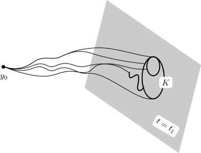
Figure 1. The funnel of a two dimensional time dependent ODE through $y_{0}$ and its cross-section $K$ in the time-$t_{1}$ plane.

The funnel section consists of the points $y_{1}\in\mathbb{R}^{m}$ that are accessible from $y_{0}$ by a solution starting from $y_{0}$ at time $t_{0}$ and arriving at $y_{1}$ at time $t_{1}$.

The classical theorem about funnel sections is due to H. Kneser. It states that $K_{t_{1}}$ is a continuum (i.e., is nonempty, compact, and connected) if $f:\mathbb{R}^{m+1}\rightarrow\mathbb{R}^{m}$ is continuous and has compact support. See [2] and [4].

In [4] the first author investigated the question: “which continua are funnel sections?” The main answers were

• The planar continuum consisting of an outward spiral and its limit circle is not a funnel section of any $m$-dimensional ODE.

• Every continuum in $\mathbb{R}^{m}$ whose complement is diffeomorphic to $\mathbb{R}^{m}\setminus\{0\}$ is a funnel section of an $m$-dimensional ODE.

• All piecewise smooth, compact, connected polyhedra in $\mathbb{R}^{m}$ are funnel sections of $m$-dimensional ODEs.

(b) provides a great many pathological continua as funnel sections. For example, all non-separating planar continua are funnel sections. This includes the topologist’s sine curve, the bucket handle, and the pseudo-arc (which contains no ordinary arcs). (c) implies that all compact smooth manifolds are funnel sections.

An obvious question remains open: Is the property of being a funnel section topological, or does it depend on how the continuum is embedded in $\mathbb{R}^{m}$? The simplest case is the circle, where the question becomes: “Is every Jordan curve a funnel section of a two dimensional ODE?” In this paper we answer the question affirmatively under some extra hypotheses, and point out the difficulties in general. We also expand on some remarks in [4].

2. Smooth Pierceability

An arc pierces a separating plane continuum $K$, such as a Jordan curve, if it meets $K$ at a single point and passes from one complementary component of $K$ to another. If the arc is smooth it smoothly pierces $K$. Planar Jordan curves are everywhere pierceable and smooth Jordan curves are everywhere smoothly pierceable.

Theorem 1.

If a planar Jordan curve is smoothly pierceable at some point then it is a funnel section of a two dimensional ODE.

Patching Lemma.

If $K$ is a funnel section of an $m$-dimensional ODE and $p\in\mathbb{R}^{m}$ is given then there exists a continuous $g:\mathbb{R}^{m+1}\rightarrow\mathbb{R}^{m}$ with compact support contained in $[0,1]\times\mathbb{R}^{m}$ such that $K=K_{1}(0,p,g)$.

Proof.

This is Proposition 2.4 of [4]. It lets us patch funnels together, one to the next. ∎

Proof of Theorem 1..

Let $J\subset\mathbb{R}^{2}$ be a Jordan curve pierced at $p$ by a smooth arc $A$. We may assume $p$ is the origin and $A$ contains the horizontal segment $[-1,1]\times\{0\}$. Let $\beta:\mathbb{R}\rightarrow[0,1)$ be a smooth bump function such that the eye-shaped region $S$ between the graphs of $-\beta$ and $\beta$ is as in Figure 2.

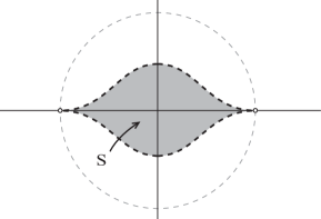
Figure 2. The eye-shaped region $S$.

There is a smooth map $\Psi:\mathbb{R}^{2}\setminus S\rightarrow\mathbb{R}^{2}$ closing the eye. It sends the vertical segment $x\times[\beta(x),1]$ to $x\times[0,1]$, is symmetric with respect to $y\mapsto-y$, and is the identity outside the unit disc $\mathbb{D}$. Except for the fact that $\Psi(x,\beta(x))=(x,0)=\Psi(x,-\beta(x))$, $\Psi$ is a diffeomorphism.

The map $\Psi^{-1}:\mathbb{R}^{2}\setminus(-1,1)\times 0$ opens the eye and sends $J\setminus 0$ to a an open arc. Let $J^{\displaystyle*}=\Psi^{-1}(J\setminus 0)\cup(0,\beta(0))\cup(0,-\beta(0))$. It is a compact planar arc, so it is a funnel section: $J^{\displaystyle*}=K_{1}(0,p,f)$ for some $p\in\mathbb{R}^{2}$ and some $f=f(t,x,y)$ with compact support in $[0,1]\times\mathbb{R}^{2}$. (Here we used the Patching Lemma and the fact from [4] that every planar continuum whose complement is diffeomorphic to $\mathbb{R}^{2}\setminus 0$ is a funnel section.)

Next, we gradually close the eye as $t$ varies from $t=1$ to $t=2$. There is a continuous vector field $g=g(t,x,y)$ tangent to the vertical lines $x\times\mathbb{R}$ whose forward trajectories on $[1,2]\times x\times[-1,1]$ are shown in Figure 3.

Figure 3. A $g$-trajectory starting at $(1,x,y)$ with $\lvert y\rvert\geq\beta(x)$ ends at $(2,\Psi(x,y))$.

The time-one map of the forward $g$-flow is $\Psi$. See Figure 4.

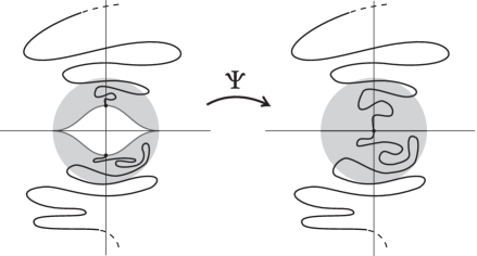
Figure 4. $\Psi$ closes the eye.

Thus $J$ is a funnel section, $J=K_{2}(0,p,f+g)$. ∎

Theorem 2.

There exist planar Jordan curves, smoothly pierceable at no points. Some of them are funnel sections.

See Section 5 for the proof of the second assertion.

Remark.

It is natural to expect that unions and intersections of funnel sections of $m$-dimensional ODEs are funnel sections of $m$-dimensional ODEs. The union case is an open question, while the intersection assertion is false. In fact, if it were known that the union of two funnel sections of $2$-dimensional ODEs is a funnel section of a $2$-dimensional ODE then it would follow at once that every planar Jordan curve $J$ is a funnel section of a $2$-dimensional ODE. For $J$ is the union of two arcs, each being a funnel section of a $2$-dimensional ODE by (b) in Section 1. See Section 4 for the union question when it is permitted to raise the dimension.

To understand the funnel intersection question, consider the outward spiral together with its limit circle, $\overline{S}$. It is not a funnel section, but its one-point suspension $T$ is one. For the complement of $T$ in $\mathbb{R}^{3}$ is diffeomorphic to the complement of a point. The closed unit disc $\overline{\mathbb{D}}\subset\mathbb{R}^{2}\subset\mathbb{R}^{3}$ is a funnel section, but $\overline{S}=T\cap\overline{\mathbb{D}}$ is not.

3. Nowhere smoothly Pierceable Jordan curves

It is not surprising that there exist planar Jordan curves which are nowhere smoothly pierceable. We prove slightly more.

Theorem 3.

There are planar Jordan curves that are nowhere pierceable by paths of finite length. Some of them are funnel sections.

See Section 5 for the proof of the second assertion.

If $J\subset S^{2}$ is a Jordan curve that separates the north and south poles and $\gamma$ is a path from one pole to the other that pierces $J$ then we call $\gamma$ a polar path for $J$. Every polar path has length $\geq\pi$. The resistance of $J$ is

$$r(J)=\inf\{\ell(\gamma):\gamma\textrm{ is a polar path for }J\}$$

where $\ell(\gamma)$ is the length of $\gamma$.

The greater the resistance, the longer it takes a point to travel at unit speed from pole to pole crossing $J$ just once. The equator has resistance $\pi$. Approximating it by a Jordan curve $B$ made of many small consecutive buttons as in Figure 5 does not increase the resistance, but subsequently adding zippers across the buttons as in Figure 6 increases the resistance as much as we want.

Figure 5. Part of a button curve $B$.

Figure 6. Part of a zippered button curve – a resistor curve.

Resistance Theorem.

There exist Jordan curves with infinite resistance.

Proof..

Modify the equator by approximating it with a smooth resistor curve $R_{1}$ having resistance $>\pi$. Then approximate $R_{1}$ with a resistor curve $R_{2}$ having resistance $>2\pi$, etc., and take a limit. The details appear below. ∎

Lemma 4.

There is a diffeomorphism $\sigma:[0,1]^{2}\rightarrow[0,1]^{2}$ such that $\sigma$ is the identity on a neighborhood of the boundary and $\sigma$ carries the rectangle $[2/5,3/5]\times[0,1]$ to an S-shaped strip $S$ such that for every path $\gamma(t)=(x(t),y(t))$ in $S$ connecting the top and bottom of $S$, $0\leq t\leq 1$, we have

$$\int_{0}^{1}\lvert x^{\prime}(t)\rvert\,dt\geq 1\ .$$

Proof..

See Figure 7.

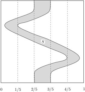
Figure 7. The S-shaped strip $S$.

∎

Lemma 5.

Given $L>0$, there is a diffeomorphism $\zeta:[0,a]\times[0,b]\rightarrow[0,a]\times[0,b]$ such that $\zeta$ is the identity on a neighborhood of the boundary and $\zeta$ carries the rectangle $[2a/5,3a/5]\times[0,b]$ to a zipper strip $Z$ such that every path $\gamma$ in $Z$ connecting the top and bottom of $Z$ has length $\geq L$.

Proof..

Reduce the unit square to a rectangle $[0,a]\times[0,b/n]$ with $n\geq L/a$. Stack $n$ copies of the reduced strip diffeomorphism $\sigma$ from Lemma 4 to form $\zeta$ and $Z$. The length of $\gamma$ is at least $na\geq L$. See Figure 8 in which $a=1$, $b=1/2$, and $n=4$. ∎

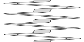
Figure 8. A stack of four unit-length S-strips forms a zipper strip $Z$ with $r(Z)\geq 4$.

Let $C$ be the cylinder $S^{1}\times[-1,1]$ and let $J$ be a Jordan curve that separates its top and bottom. As for paths on the sphere, a path on the cylinder connecting the top and bottom is polar for $J$ if it meets $J$ exactly once, and the resistance of $J$ is the infimum of the lengths of the polar paths. Let $E$ be the equator of $C$.

Lemma 6.

Given $\epsilon>0$ and $L>0$, there is a diffeomorphism $\varphi:C\rightarrow C$ in the $\epsilon$-neighborhood of the identity such that $\varphi$ is the identity off the $\epsilon$-neighborhood of $E$, and $J=\varphi(E)$ has resistance $>L$.

Proof..

Choose $a=1/n\leq\epsilon/2$ and divide the cylinder $C_{a}=S^{1}\times[-a,a]$ into $n$ squares of size $a\times a$. Draw a button curve $B$ with $n$ buttons, one in each square. There is a diffeomorphism $\phi:C\rightarrow C$ sending each square to itself such that $\phi(E)=B$ and $\phi$ is the identity off $C_{a}$.

Then draw $2n$ rectangles $\rho,\rho^{\prime}$ of length $a/2$ and height $b$ as shown in Figure 9.

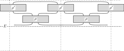
Figure 9. Zipper strips are glued into the rectangles $\rho,\rho^{\prime}\subset C_{a}$.

In each rectangle, replace the identity map by the zipper diffeomorphism constructed in Lemma 5. This gives a diffeomorphism $\zeta:C\rightarrow C$. The composite $\varphi=\zeta\circ\phi$ $\epsilon$-approximates the identity and fixes all points off $C_{a}$. Every polar path for $J=\varphi(E)$ must travel through an entire zipper strip and therefore has length $>L$. ∎

Let $\mathcal{J}_{0}$ be the collection of Jordan curves on the 2-sphere that separate the poles.

Lemma 7.

With respect to the Hausdorff metric, the resistance function is lower semi-continuous at smooth Jordan curves in $\mathcal{J}_{0}$.

Proof..

Let $J_{n}$ be a sequence of Jordan curves in $\mathcal{J}_{0}$ that converges to $J\in\mathcal{J}_{0}$ with respect to the Hausdorff metric. If $J$ is smooth we claim that $r(J)\leq\displaystyle\liminf_{n\rightarrow\infty}r(J_{n})$. We refer to points on the south side of a curve in $\mathcal{J}_{0}$ as “below” and those on the north side as “above.”

Consider the $\epsilon$-tubular neighborhood $N=N_{\epsilon}$ of $J$. It is an annulus bounded by smooth Jordan curves $J_{a}$ and $J_{b}$ above and below $J$. The normals to $J$ give smooth projections $\pi_{a}:N\rightarrow J_{a}$, $\pi_{b}:N\rightarrow J_{b}$. As $\epsilon\rightarrow 0$, the norms of $(D\pi_{a})_{x}$ and $(D\pi_{b})_{x}$ for $x\in N$ tend uniformly to $1$. Thus, if $\nu$ is a smooth path in $N$ then the length ratio satisfies

$$\liminf_{\epsilon\rightarrow 0}\frac{\ell(\nu)}{\ell(\pi_{a}(\nu))}\geq 1\qquad\liminf_{\epsilon\rightarrow 0}\frac{\ell(\nu)}{\ell(\pi_{b}(\nu))}\geq 1\ ,$$

uniformly $\nu\subset N$.

Fix a small $\epsilon>0$ and choose a polar path $\gamma_{n}$ for $J_{n}$ whose length is approximately $r(J_{n})$. For large $n$, $J_{n}\subset N$ and $J_{n}$ separates the boundary curves $J_{a},J_{b}$ of $N$. By approximation, we can assume that $\gamma_{n}$ is smooth except at the point $p_{n}\in J_{n}$ where it crosses $J_{n}$, and that $\gamma_{n}$ is transverse to $\partial N$. We form a polar path $\rho_{n}$ for $J$ as follows. (It will not be much longer than $\gamma_{n}$.)

The polar path $\gamma_{n}$ for $J_{n}$ goes from the north pole to the south pole, and $J_{n}$ splits it as $\gamma_{n}=\alpha\cup\beta$ where $\alpha$ goes from the north pole to $p_{n}$ and $\beta$ goes from $p_{n}$ to the south pole. Since $J_{n}$ separates the boundary curves of $N$, $\alpha$ lies above $J_{b}$ and $\beta$ lies below $J_{a}$. Transversality implies that $\alpha$ splits as

$$\alpha=\alpha_{1}\cup\nu_{1}\cup\dots\cup\alpha_{k}\cup\nu_{k}$$

where each $\alpha_{j}$ lies above $J_{a}$ and each $\nu_{j}$ lies in $N$. The curve

$$\rho_{a}=\alpha_{1}\cup\pi_{a}(\nu_{1})\cup\dots\cup\alpha_{k}\cup\pi_{a}(\nu_{k})$$

lies above or on $J_{a}$ and has length not much greater than $\ell(\alpha)$. (In fact, it is likely that $\ell(\rho_{a})$ is much less than $\ell(\alpha)$.) See Figure 10.

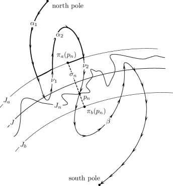
Figure 10. $J_{a}$ splits $\alpha$ as $\alpha=\alpha_{1}\cup\nu_{1}\cup\alpha_{2}\cup\nu_{2}$. The path $\rho_{a}$ is drawn thick.

In the same way we form from $\beta$ a path $\rho_{b}$ that lies below or on $J_{b}$ and has length not much greater than $\ell(\beta)$. The path $\rho_{a}$ ends at the point $\pi_{a}(p_{n})$ while $\rho_{b}$ starts at the point $\pi_{b}(p_{n})$. Let $\sigma_{n}=[\pi_{a}(p_{n}),\pi_{b}(p_{n})]$ be the normal segment of $N$ that passes through $p_{n}$. Thus,

$$\rho_{n}=\rho_{a}\cup\sigma_{n}\cup\rho_{b}$$

is a polar path $J$ and its length is not much greater than $\ell(\gamma_{n})$. It follows that $r(J)\leq\displaystyle\liminf_{n\rightarrow\infty}r(J_{n})$. ∎

Remark.

The resistance function is not upper semicontinuous. There exist resistor curves approximating the equator arbitrarily well that have large resistance.

Question.

Is the preceding lemma true without the assumption that $J$ is smooth? That is, if $J_{n}\rightarrow J$ in $\mathcal{J}_{0}$ and there are polar paths $\gamma_{n}$ for $J_{n}$ of length $\leq r$, is there a polar path for $J$ of length $\leq r+\epsilon$?

Lemma 7 uses the Hausdorff metric on $\mathcal{J}_{0}$. A finer topology is defined as follows. Every parameterization of a Jordan curve is an embedding $f:S^{1}\rightarrow S^{2}$, and every $f$ extends to a homeomorphism $F:S^{2}\rightarrow S^{2}$. (We think of the circle as the equator of the sphere.) The space $\mathcal{H}$ of self-homeomorphisms of the sphere has a natural metric

$$D(F,G)=\lVert F-G\rVert+\lVert F^{-1}-G^{-1}\rVert\ ,$$

where $\lVert F_{1}-F_{2}\rVert=\sup\{\lvert F_{1}(x)-F_{2}(x)\rvert:x\in S^{2}\}$ is $C^{0}$-distance. With respect to $D$, $\mathcal{H}$ is complete, and the subset

$$\mathcal{H}_{0}=\{F\in\mathcal{H}:F(S^{1})\textrm{ separates the poles}\}$$

is closed in $\mathcal{H}$.

Lemma 8.

For the generic $F\in\mathcal{H}_{0}$, $F(S^{1})$ has infinite resistance.

Proof..

It suffices to check that for every $L>0$,

$$\mathcal{H}_{0}(L)=\{F\in\mathcal{H}:F(S^{1})\textrm{ has resistance $>L$}\}$$

contains an open dense subset. Let $F_{0}\in\mathcal{H}_{0}$ be given. It can be approximated in $\mathcal{H}_{0}$ by a diffeomorphism $F_{1}$. The tubular neighborhood of the smooth Jordan curve $J_{1}=F_{1}(S^{1})$ is diffeomorphic to the cylinder, so Lemma 6 provides a diffeomorphism $F_{2}$ that approximates the identity and $J=F_{2}(J_{1})$ has resistance $>L$. Then $F=F_{2}\circ F_{1}$ approximates $F_{1}$ and lies in $\mathcal{H}_{0}(L)$. Hence $\mathcal{H}_{0}(L)\cap C^{\infty}$ is dense in $\mathcal{H}_{0}$. For each $F\in\mathcal{H}_{0}(L)\cap C^{\infty}$, $J=F(S^{1})$ is smooth, so Lemma 7 implies that for all $G\in\mathcal{H}_{0}$ near $F$, $G(S^{1})$ has resistance $>L$. That is, $\mathcal{H}_{0}(L)$ contains a neighborhood of $F$. Hence $\mathcal{H}_{0}(L)$ contains an open dense subset of $\mathcal{H}_{0}$, and $\bigcap_{L\in\mathbb{N}}\mathcal{H}_{0}(L)$ is residual; that is, for the generic $F\in\mathcal{H}_{0}$, $J=F(S^{1})$ has infinite resistance. ∎

Proof of the Resistance Theorem..

Since residual subsets of a complete nonempty metric space are nonempty, Lemma 8 provides many Jordan curves of infinite resistance. ∎

Remark.

A Jordan curve $J$ of infinite resistance is nowhere smoothly pierceable. For if $\nu$ is a smooth path piercing $J$ then we can choose a smooth path $\alpha$ from the north pole to one endpoint of $\nu$, and a smooth path $\beta$ from the other endpoint of $\nu$ to the south pole, such that $\alpha$ and $\beta$ are disjoint from $J$. Then the combined path $\alpha\cup\nu\cup\beta$ is polar with finite length, contradicting $r(J)=\infty$.

Remark.

There is nothing special about the poles of the sphere. For any distinct $p,q\in S^{2}$ we can consider the set $\mathcal{H}_{pq}$ of homeomorphisms $F\in\mathcal{H}$ such that $F(S^{1})$ separates $p$ from $q$. Letting $p,q$ vary in a countable dense subset of the sphere, we infer a stronger looking version of the Resistance Theorem.

Theorem 9.

For the generic $F\in\mathcal{H}$, the Jordan curve $J=F(S^{1})$ offers infinite resistance to all paths piercing it.

4. One Dimension Up

The outward spiral together with its limit circle, $\overline{S}$, is not a funnel section of any continuous $2$-dimensional ODE, and in fact it is not a funnel section of any continuous $m$-dimensional ODE. Raising the permitted dimension has no effect on this property of $\overline{S}$. However, some funnel questions get easier if the dimension can be increased.

Theorem 10.

The image of a funnel section under projection is a funnel section.

Proof.

There is a continuous function $g(t,x)$ on $\mathbb{R}^{2}$ such that the trajectories of $x^{\prime}=g$ are as in Figure 3: All trajectories $x(t)$ that begin in the interval $[-1,1]$ at time $t=1$ end at $0$ by time $t=2$. The support of $g$ is compact and contained in $[1,2]\times\mathbb{R}$. This gives a local projection.

Suppose that $K=K_{1}(0,p,f)$ is a subset of the unit $m$-cube $Q$ for some continuous $f=f(t,x^{1},\dots,x^{m})$ with compact support in $[0,1]\times\mathbb{R}^{m}$. Let $\pi:\mathbb{R}^{m}\rightarrow\mathbb{R}^{m-1}$ be the projection that kills the span of the last variable $x^{m}$. Then

$$\pi(K)=K_{2}(0,p,f+g)$$

where $g$ is the vector field on $\mathbb{R}^{m}$,

$$(0,\dots,0,g(t,x^{m}))=g(t,x^{m})\frac{\partial}{\partial x^{m}}\ .$$

Projections into higher codimension subspaces are handled by induction. ∎

Corollary.

Every planar Jordan curve is a funnel section of $3$-dimensional ODE.

Proof.

Let $h:[0,2\pi]\rightarrow J$ parametrize the Jordan curve $J\subset\mathbb{R}^{2}$, and define $g:[0,2\pi]\rightarrow\mathbb{R}^{3}$ by

$$g(\theta)=(h(\theta),\theta)\ .$$

$g([0,2\pi])$ is an arc $K$ in $\mathbb{R}^{3}$. Its complement is diffeomorphic to the complement of a point, so it is a funnel section of a $3$-dimensional ODE. Theorem 10 implies that $\pi(K)=J$ is a funnel section of a $3$-dimensional ODE. ∎

In fact, we have established something a bit more general.

Theorem.

Peano continua in $\mathbb{R}^{m}$ are funnel sections in one dimension up.

Proof.

A Peano continuum $X$ is the continuous image of an interval. (Equivalently, by the Hahn-Mazurkiewicz Theorem a Peano continuum is a compact Hausdorff space which is connected and locally connected.) Jordan curves are Peano continua. If $h:[0,2\pi]\rightarrow X\subset\mathbb{R}^{m}$ is a continuous surjection then $\theta\mapsto g(\theta)=(h(\theta),\theta)$ is a homeomorphism from the interval to an arc $K\subset\mathbb{R}^{m+1}$. The latter is a funnel section of an $(m+1)$-dimensional ODE, and by Theorem 10, so is $X=\pi(K)$. ∎

Corollary.

The Hawaiian earring is a funnel section of a $3$-dimensional ODE.

Proof.

The Hawaiian earring is a planar Peano continuum. ∎

Remark.

It is not hard to show directly that the Hawaiian earring is also a funnel section of a $2$-dimensional ODE.

Theorem 11.

If a continuum is a union of two funnel sections then it is a funnel section in one dimension up.

Proof.

Suppose that $A,B\subset\mathbb{R}^{m}$ are funnel sections for $m$-dimensional ODEs, $A=K_{1}(0,p,f)$ and $B=K_{1}(0,q,g)$ for continuous $f,g:\mathbb{R}^{m+1}\rightarrow\mathbb{R}^{m}$ having compact support in $[0,1]\times\mathbb{R}^{m}$, and $c\in A\cap B$. It suffices to construct a funnel section $K$ consisting of a line segment $L=c\times[0,3]$ and copies of $A$, $B$ as shown in Figure 11.

Figure 11. The configuration of the desired funnel section is $K=A\times 0\;\cup\;L\;\cup\;B\times 3$.

For then Theorem 10 implies $\pi(K)=A\cup B$ is a funnel section of an $(m+1)$-dimensional ODE.

Without loss of generality we assume that the interior of the unit cube $Q=Q^{m+1}$ contains the supports of $f$, $g$, and the funnels through $p$ and $q$.

We write $(t,x,z)\in\mathbb{R}\times\mathbb{R}^{m}\times\mathbb{R}$ systematically. It is easy to construct a continuous $h_{0}:\mathbb{R}^{m+2}\rightarrow\mathbb{R}^{m+1}$ with compact support in $[-1,0]\times\mathbb{R}^{m+1}$ such that

$$\begin{split}K_{0}(-1,p,h_{0})&=L_{0}\\ &=[(0,p,0),(0,p,1)]\cup[(0,p,1),(0,q,2)]\cup[(0,q,2),(0,q,3)]\ .\end{split}$$

$L_{0}$ is the broken line in the $t=0$ plane from $(0,p,0)$ to $(0,q,3)$ having vertices $(0,p,1)$ and $(0,q,2)$. Then we will construct $h$ so that $K_{1}(0,L_{0},h)=K$. This gives $K_{1}(-1,p,h_{0}+h)=K$.

First we fix $f$- and $g$-solutions $a(t)$ and $b(t)$ such that $a(0)=p$, $b(0)=q$, and $a(1)=c=b(1)$. Then we construct $h$ on the three slabs $0\leq z\leq 1$, $1\leq z\leq 2$, $2\leq z\leq 3$ as follows. We think of $z$ as an “external homotopy variable” by requiring that the $z$-component of $h$ is identically zero. This forces $h$-solutions to stay in $z=const.$ planes. For clarity we drop the zero $z$-component from the notation for $h$ and write $h(t,x,z)$ as an $m$-vector. Choose a bump function $\beta(t,x,z)$ on the bottom slab $0\leq z\leq 1$ such that

• $\beta=1$ on the set $\{(t,x,z)\in Q\times(0,1]:\lvert x-a(t)\rvert\leq 2z\}$.

• $\beta=0$ on the set $\{(t,x,z)\in Q\times[0,1]:\lvert x-a(t)\rvert\geq 4z\}$.

• $0\leq\beta\leq 1$ otherwise.

See Figure 12, and note that $\beta=1$ on the set $Q\times 1$.

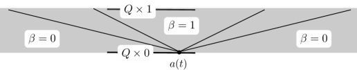
Figure 12. $\beta$ is continuous except at $(t,a(t),0)$.

Although $\beta$ is discontinuous at $(t,a(t),0)$, the average

$$h(t,x,z)=\beta(t,x,z)f(t,a(t))+(1-\beta(t,x,z))f(t,x)$$

is continuous on the whole slab. The set $N_{z}=\{(t,x,z):\lvert x-a(t)\rvert<2z\}$ is an open tubular neighborhood of the curve $(t,a(t),z)$. On $N_{z}$, $\beta=1$.

We claim that for $0<z\leq 1$, $a(t)$ is the unique solution of

$$x^{\prime}=h(t,x,z)\quad x(0)=p\ .$$

Let $x(t)$ be any solution of this equation. It starts out in $N_{z}$, where $\beta=1$ implies $h(t,x,z)=f(t,a(t))$, a function that does not depend on $x$. Thus, for small $t$ the solution is unique and given by integration

$$x(t)=p+\int_{0}^{t}f(s,a(s))\,ds\ ,$$

which is the same as $a(t)$. Thus $x(t)=a(t)$ for small $t$. Since $a(t)$ always lies in $N_{z}$, equality continues and we get uniqueness.

In terms of funnels, this shows that

$$K_{1}(0,p\times[0,1],h)=A\times 0\;\;\cup\;\;c\times[0,1].$$

The same construction on the top slab gives

$$K_{1}(0,q\times[2,3],h)=B\times 3\;\;\cup\;\;c\times[2,3]\ .$$

We fill in the middle slab by linear interpolation. For $1\leq z\leq 2$ we set

$$h(t,x,z)=(2-z)h(t,x,z=1)+(z-1)h(t,x,z=2)$$

On the cube $Q\times[1,2]$, $h$ does not depend on $x$. It is

$$h(t,x,z)=(2-z)h(t,a(t),z=1)+(z-1)h(t,b(t),z=2)\ .$$

Both curves $a(t)$ and $b(t)$ stay interior to the unit cube $Q$, and so does their convex combination

$$c(t)=(2-z)a(t)+(z-1)b(t)\ .$$

Then $h(t,c(t),z)=(2-z)h(t,a(t),z=1)+(z-1)h(t,b(t),z=2)$ because $h(t,c(t),z)$ does not depend on $c(t)$, so

$$\begin{split}c(t)&=(2-z)\Big{(}p+\int_{0}^{t}h(s,a(s),z=1)\,ds\Big{)}\\ &+(z-1)\Big{(}q+\int_{0}^{t}h(s,b(s),z=2)\,ds\Big{)}\\ &=(2-z)p+(z-1)q+\int_{0}^{t}h(s,c(s),z)\,ds\end{split}$$

is the unique $h$-solution starting at the point $c(0)=(0,(2-z)p+(z-1)q,z)$ on the middle segment of $L_{0}$. Since $a(1)=c=b(1)$, we have $c(1)=c$. In the middle slab the trajectories through the broken segment $L_{0}$ end at the vertical segment $L$.

Finally, we extend $h$ above and below $\mathbb{R}^{m+1}\times[0,3]$ to give it compact support. The net effect is that we get the funnel section $K$ as in Figure 11, and Theorem 10 completes the proof. ∎

Remark.

By induction Theorem 11 applies to finite unions. But in general, it is not true that a countable union of funnel section must be a funnel section. For example we can decompose the closed outward spiral into countably many arcs but it is not a funnel section.

5. Diffeotopies and Funnels

A diffeotopy is a smooth curve $\varphi(t)$ in the space of diffeomorphisms, starting at the identity map when $t=0$. We often write $\varphi(t)(x)=\varphi(t,x)$.

Diffeotopies are generated by time-dependent ODEs and vice versa. More precisely, if $x(t,t_{0},x_{0})$ solves the smooth time dependent ODE

$$x^{\prime}=f(t,x)\qquad x(t_{0})=x_{0}$$

then $\varphi(t,x_{0})=x(t,0,x_{0})$ is a diffeotopy. Conversely, if $\varphi$ is a diffeotopy then $\varphi$ solves the ODE above with $f(t,x)=\varphi^{\prime}(t)(\varphi(t)^{-1}(x))$. A diffeotopy $\varphi$ defined on $[0,c)$ is said to have bounded speed if $\lvert\varphi^{\prime}(t,x)\rvert$ is uniformly bounded. In this case

$$\phi(x)=\lim_{t\rightarrow c}\varphi(t,x)$$

exists and is continuous, although it need not be a diffeomorphism. Also, if $\varphi(t,x)$ is independent from $t$ for all $t\geq c$ then the map $\phi$ defined by $x\mapsto\varphi(c,x)=\phi(x)$ is the transfer map of the diffeotopy. It is the ultimate effect of the diffeotopy on $x$.

Theorem 12.

Suppose that $A$ is a funnel section and there is a diffeotopy $\varphi$ of bounded speed on $[0,1)$ whose time one map carries $A$ onto $B$. Then $B$ is a funnel section.

Proof.

By assumption there is an ODE

$$x^{\prime}=f(t,x)\quad x(0)=p$$

whose funnel has cross-section $A$ at time $1$. By Proposition 2.4 of [4] we may assume that $f$ has compact support in $[0,1]\times\mathbb{R}^{m}$. The diffeotopy $\varphi$ gives a second ODE,

$$x^{\prime}=g(t,x)$$

whose solutions give a funnel from $0\times A$ to $1\times B$. Since $\varphi$ has bounded speed, if we reparameterize time as $\tau(t)=t^{2}(2-t)^{2}$ then the diffeotopy $\psi(t,y)=\varphi(\tau(t),y)$ has

$$\lvert\psi^{\prime}(t,y)\rvert=\lvert\varphi^{\prime}(\tau(t),y)\rvert\tau^{\prime}(t)\leq M\tau^{\prime}(t)$$

where $M$ is the maximum speed of $\varphi$. That is, $\psi$ is generated by an ODE which converges to zero as $t\rightarrow 1$. This lets us assume $g:\mathbb{R}^{m+1}\rightarrow\mathbb{R}^{m}$ is continuous and has compact support in $[0,1]\times\mathbb{R}^{m}$. Set

$$h(t,x)=f(t,x)+g(t-1,x)\ .$$

Then $K_{2}(0,p,h)=B$. ∎

Proof of Theorems 2 and 3.

Since infinite resistance implies nowhere smoothly pierceable, it suffices to prove Theorem 3: there exist Jordan curves of infinite resistance, some of which are funnel sections. The first assertion is proved in Section 3. It remains to prove that some Jordan curves of infinite resistance are funnel sections. By Theorem 12 it is enough to find a diffeotopy of bounded speed from the circle to some Jordan curve of infinite resistance. For the circle is a funnel section.

We fix a sequence $(t_{n})$ such that $0=t_{0}<t_{1}<\dots$ and $t_{n}\rightarrow 1$ as $n\rightarrow\infty$. Then we construct a sequence of smooth diffeotopies $\varphi_{n}$ on $S^{2}$ such that $\varphi_{n}$ is supported in the time interval $(t_{n},t_{n+1})$. The transfer map $\phi_{n}$ is a diffeomorphism $S^{2}\rightarrow S^{2}$ and we arrange things so that the composed transfer map $\phi_{n}\circ\cdots\circ\phi_{0}$ converges to a homeomorphism sending the equator of $S^{2}$ to a Jordan curve of infinite resistance. The construction is by induction.

First we make a general construction for any fixed smooth Jordan curve $J\subset S^{2}$ that separates the poles and has $r(J)>\alpha$. Lemma 7 provides a $\delta=\delta(J)$ such that if $J^{\prime}$ is a Jordan curve that separates the poles and has $d_{H}(J,J^{\prime})<\delta$ then $r(J^{\prime})>\alpha$. Lemmas 5 and 6 imply that there is a diffeotopy $\varphi$ such that

• $\varphi$ is supported in a thin tubular neighborhood of $J$ and $\lvert\varphi^{\prime}\rvert$ is arbitrarily small.

• The transfer map $\phi$ and its inverse $\phi^{-1}$ are arbitrarily close to the identity map in the $C^{0}$ sense.

• The smooth Jordan curve $\phi(J)$ separates the poles and $d_{H}(J,\phi(J))<\delta(J)/2$.

• $r(\phi(J))>\alpha+1$.

Start with $J_{0}$ equal to the equator of $S^{2}$. It has $r(J_{0})=\pi$. The identity diffeotopy $\varphi_{0}$ has an identity transfer map $\phi_{0}$ and it sends the equator $J_{0}$ to itself, i.e., $J_{1}=\phi_{0}(J_{0})=J_{0}$. Trivially, $r(J_{1})>1$.

Next, applying the preceding construction to $J_{1}$, we find a diffeotopy $\varphi_{1}$ supported on $(t_{1},t_{2})\times N$ where $N$ is an equatorial band, such that the transfer map $\phi_{1}$ carries $J_{1}$ to a smooth Jordan curve $J_{2}=\phi_{1}(J_{1})$. Since the poles stay fixed during the diffeotopy, $J_{2}$ separates them. The construction permits

• $\lvert\varphi_{1}^{\prime}\rvert<1$.

• $\lvert\phi_{1}(x)-x\rvert<1/2$ and $\lvert\phi_{1}^{-1}(x)-x\rvert<1/2$ for all $x\in S^{2}$.

• $r(J_{2})>2$. (This is trivial since the resistance is always $\geq\pi$.)

Inductively, assume we have defined $\varphi_{n-1}$ with time support in $(t_{n-1},t_{n})$ and transfer map $\phi_{n-1}$. Then $J_{n}=\phi_{n-1}(J_{n-1})$ is defined. Working in a thin tubular neighborhood of $J_{n}$ we construct a diffeotopy $\varphi_{n}$ such that

• $\lvert\varphi_{n}^{\prime}\rvert<1/n$.

• For all $x\in S^{2}$, the composed transfer maps and their inverses satisfy

  $$\begin{split}\lvert\phi_{n}\circ\phi_{n-1}\circ\cdots\circ\phi_{1}(x)-\phi_{n-1}\circ\cdots\circ\phi_{1}(x)\rvert<\frac{1}{2^{n}}\\ \lvert\phi_{1}^{-1}\circ\cdots\phi_{n-1}^{-1}\circ\phi_{n}^{-1}(x)-\phi_{1}^{-1}\circ\cdots\phi_{n-1}^{-1}(x)\rvert<\frac{1}{2^{n}}\end{split}$$

• If $J_{n+1}=\phi_{n}(J_{n})$ then

  $$d_{H}(J_{n},J_{n+1})<\min\Big{(}\frac{\delta(J_{1})}{2^{n}},\dots,\frac{\delta(J_{n})}{2}\Big{)}\ .$$

By (a_n) the diffeotopy $\bigcup\varphi_{n}$ has bounded speed on $0\leq t<1$.

Consider $\Phi_{n}=\phi_{n}\circ\cdots\circ\phi_{1}$. By (b_n) we have

$$\lVert\Phi_{n}-\Phi_{n-1}\rVert<\frac{1}{2^{n}}\quad\textrm{and}\quad\lVert\Phi_{n}^{-1}-\Phi_{n-1}^{-1}\rVert<\frac{1}{2^{n}}\ ,$$

so the sequence $(\Phi_{n})$ is Cauchy in the space of homeomorphisms of $S^{2}$, and it converges uniformly to a homeomorphism $\Phi$ of $S^{2}$. Let $J=\Phi(J_{0})$. It is a Jordan curve in $S^{2}$. Since the poles stay fixed under the diffeotopies, $J$ separates them.

By (c_n),

$$d_{H}(J_{n},J)\leq\sum_{k=n}^{\infty}d_{H}(J_{k},J_{k+1})<\sum_{k=1}^{\infty}\frac{\delta(J_{n})}{2^{k}}=\delta(J_{n})\ ,$$

which implies that $r(J)>n$. Hence $r(J)=\infty$. Since we arrived at $J$ by a funnel from $p$ to the equator, followed by a funnel from the equator to $J$, $J$ is a funnel section. ∎

Remark.

The diffeotopy produced above ends with a homeomorphism of the sphere to itself and is therefore reversible. The reverse funnel from the Jordan curve leads back to the equator, $K_{0}(1\times J)=E$, and in the terminology of [4] we have a “funnel cobordism” between $E$ and $J$ .

Remark.

We do not know whether for every planar Jordan curve $J$ there is a diffeotopy of bounded speed that starts at the equator and ends at $J$. If we did then we would know that every planar Jordan curve is a funnel section.

The proof of Theorem 3 above establishes the following approximation result.

Theorem 13.

A smooth Jordan curve can be approximated by other smooth Jordan curves having arbitrarily large resistance. That is, if $h:S^{1}\rightarrow\mathbb{C}$ sends $S^{1}$ diffeomorphically onto a Jordan curve $J$ and $\delta,L>0$ are given, then there is an $h_{1}:S^{1}\rightarrow\mathbb{C}$ sending $S^{1}$ diffeomorphically onto a smooth Jordan curve $J_{1}$ such that $\lVert h-h_{1}\rVert<\delta$ and $r(J_{1})>L$.

6. An Alexander Horned Sphere is a funnel section

Consider instead of a Jordan curve, an Alexander Horned sphere $A$ [1]. We claim there is a diffeotopy $\varphi$ on $[0,1)\times\mathbb{R}^{3}$ of bounded speed that starts at the sphere $S^{2}$ and ends at $A$. Theorem 12 and the fact that $S^{2}$ is a funnel section imply that $A$ is a funnel section. The time one map of the diffeotopy is continuous but it cannot be a homeomorphism because the complementary domains of $S^{2}$ and $A$ are not homeomorphic.

The word “an” indicates that, as with Jordan curves, we do not know that every Alexander Horned Sphere is a funnel section, only that some of them are. Theorem 12 is what may have been intended on page 283 of [4] by the phrase “Using the methods of Section 4, it also follows that the usual Alexander Horned Sphere is a funnel section and so is the [closure of the] set it bounds.”

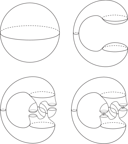
Figure 13. The sphere’s image at time $0,1/2,3/4$ and $7/8$ of the diffeotopy.

As a preliminary step we easily construct a diffeotopy $\varphi_{0}$ supported in the time interval $(0,t_{1})$ that bends the sphere into a banana shape so that the polar caps at the north and south poles become supported on a pair of parallel discs of diameter $1$ and distance $1$ apart. This is shown in the second part of Figure 13. The resulting smooth sphere is $S_{1}=\phi_{0}(S^{2})$ where $\phi_{0}$ is the transfer map of $\varphi_{0}$.

Next we define a diffeotopy $\varphi_{1}$ on the time interval $(1/2,3/4)$ that fixes all points of $S_{1}$ in the complement of the two parallel caps and moves four disjoint discs in the caps to the four smaller caps shown in the third part of Figure 13. The four discs have diameter $1/4$; the diffeotopy $\varphi_{1}$ moves them to parallel caps of diameter $1/4$ and distance $1/4$ apart. The resulting smooth sphere is $S_{2}=\phi_{1}(S_{1})$.

At the $n^{\textrm{th}}$ stage, we develop $2^{n-1}$ independent banana shapes where the spatial dimensions are reduced by the factor $1/4$ from the spatial dimensions at the previous stage, while the time interval is reduced by the factor $1/2$. This is done merely by copying and scaling the diffeotopy $\varphi_{1}$. Since the spatial reduction dominates the time reduction the speed of the combined diffeotopy $\varphi=\bigcup\varphi_{n}$ tends to zero as $t\rightarrow 1$. Hence the whole diffeotopy on $[0,1)$ starts at $S^{2}$, has bounded speed, and limits to our Alexander horned sphere as $t\rightarrow 1$. As stated at the outset, since $S^{2}$ is a funnel section, so is $A$.

The same construction done with the roles of inside and outside reversed shows that an Alexander Horned Sphere with inward curling horns is also a funnel section, as is an Alexander Horned Ball.

7. A complete metric on the space of Jordan curves

The space of homeomorphisms of a compact metric space to itself has a natural complete metric, but the same does not seem to be true for the space of topological embeddings of a compact metric space into another metric space. In the case of planar Jordan curves, we use the Riemann mapping theorem to get such a metric. Many thanks to Andy Hammerlindl and Bill Thurston for elegant suggestions regarding the construction of such a metric.

As above, let $\mathcal{J}_{0}$ denote the set of Jordan curves in $\widehat{\mathbb{C}}$ that separate the poles. Given $J\in\mathcal{J}_{0}$, Caratheodory’s Theorem supplies unique conformal bijections

$$R:\mathbb{D}\rightarrow\Omega\qquad\widetilde{R}:\mathbb{D}\rightarrow\widetilde{\Omega}$$

such that

• $\Omega$ and $\widetilde{\Omega}$ are the connected components of $\widehat{\mathbb{C}}\setminus J$ containing the south pole and north pole respectively.

• $R(0)$ is the south pole and $\widetilde{R}(0)$ is the north pole.

• If $\pi$ denotes stereographic projection then $(\pi\circ R)^{\prime}(0)$ is real and positive.

• If $\alpha$ denotes inversion $z\mapsto 1/z$ then $(\pi\circ\alpha\circ\widetilde{R})^{\prime}(0)$ is real and positive.

We refer to $R$ and $\widetilde{R}$ as the canonical Riemann maps corresponding to $J\in\mathcal{J}_{0}$.

Definition.

For $J_{1},J_{2}\in\mathcal{J}_{0}$, set

$$d(J_{1},J_{2})=\lVert R_{1}-R_{2}\rVert+\lVert\widetilde{R}_{1}-\widetilde{R}_{2}\rVert\ ,$$

where $R_{1},\widetilde{R}_{1}$ and $R_{2},\widetilde{R}_{2}$ are the canonical Riemann maps corresponding to $J_{1}$ and $J_{2}$. (Recall that $\lVert F-G\rVert$ is the $C^{0}$ distance between $F$ and $G$.) It is clear that $d$ is a metric on $\mathcal{J}_{0}$, and we call it the welding metric. For it deals with pairs $R\sqcup\widetilde{R}$ welded by $R^{-1}\circ\widetilde{R}|_{\partial\mathbb{D}}$.

Theorem 14.

The welding metric is complete.

Proof.

To show that $d$ is complete, let $(J_{n})$ be a Cauchy sequence in $\mathcal{J}_{0}$. The Riemann maps $R_{n}$ and $\widetilde{R}_{n}$ corresponding to $J_{n}$ converge uniformly to continuous maps $R$ and $\widetilde{R}$ from the closed disc into $\widehat{\mathbb{C}}$. Uniform convergence and $R_{n}(\partial\mathbb{D})=J_{n}=\widetilde{R}_{n}(\partial\mathbb{D})$ imply that

$$R(\partial\mathbb{D})=J=\widetilde{R}(\partial\mathbb{D})\ .$$

This shows that $J$ is a curve, but we don’t yet know it’s a Jordan curve, nor that $J_{n}$ converges to it with respect to $d$.

By Hurwitz’ Theorem, the restriction of $\widetilde{R}$ to the open disc is either constant or a holeomorphism – a holomorphic homeomorphism. But if $\widetilde{R}$ is constant on the open disc then by continuity and the fact that each $\widetilde{R}_{n}$ sends the origin to the north pole, $\widetilde{R}(\overline{\mathbb{D}})$ is the north pole. This implies that for $n$ large, the Jordan curve $J_{n}$ approximates the north pole, and its southern complementary region $\Omega_{n}$ approximates $\pi^{-1}(\mathbb{C})$, the sphere minus the north pole. Consequently, $\pi\circ R_{n}:\mathbb{D}\rightarrow\mathbb{C}$ converges to a holeomorphism $\mathbb{D}\rightarrow\mathbb{C}$, a contradiction to Liouville’s Theorem. Therefore $\widetilde{R}$ sends $\mathbb{D}$ holeomorphically onto a region $\widetilde{\Omega}\subset\widehat{\mathbb{C}}$ containing the north pole, and similarly, $R$ sends $\mathbb{D}$ holeomorphically onto a region $\Omega\subset\widehat{\mathbb{C}}$ containing the south pole.

We claim that $R$ and $\widetilde{R}$ are injective. Suppose not: there exist $p,q\in\overline{\mathbb{D}}$ with $p\not=q$ and $R(p)=R(q)$. We first show that $p,q\in\partial\mathbb{D}$. We know that $R$ sends the open disc $\mathbb{D}$ holeomorphically onto the region $\Omega$, so at least one of $p$ and $q$ belongs to $\partial\mathbb{D}$. If $p\in\mathbb{D}$ and $q\in\partial\mathbb{D}$ then there are points $q^{\prime}\in\mathbb{D}$ near $q$ sent to points near $R(p)$, contradicting the fact that all points near $R(p)$ are $R$-images of points near $p$.

Thus, if $R(p)=R(q)$ and $p\not=q$ then $p,q\in\partial\mathbb{D}$. Consider the radial segments $P=[0,p]$ and $Q=[0,q]$ in $\overline{\mathbb{D}}$. Their $R$-images are arcs from the south pole to $z=R(p)=R(q)$. Except for the south pole and $z$, the arcs are disjoint, so their union is a Jordan curve $H$ contained in $\Omega\cup\{z\}$. The south pole belongs to $H$ but the north pole does not. Let $U$ be the complementary region of $H$ contained in $\Omega$. (Equivalently, it is the complementary region that does not contain the north pole.) Let $V=R^{-1}(U)$. It is contained in one of the two sectors, say $S$, in $\mathbb{D}$ bounded by the radial segments $P$, $Q$, and a circular arc $A$ joining $p$ to $q$. See Figure 14.

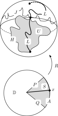
Figure 14. The Riemann map $R$ sends $\mathbb{D}$ to the southern region bounded by $J$. It also sends $V\subset S$ to $U$, $P\cup Q$ to the Jordan curve $H$, and $[0,x]$ to the southern part of the arc $L$.

Fix any $x\in A$. We have $R(x)\in J$, so there is at least one $\widetilde{x}\in\partial\mathbb{D}$ with $\widetilde{R}(\widetilde{x})=R(x)$. Then $L=R([0,x])\cup\widetilde{R}([0,\widetilde{x}])$ is an arc in $S^{2}$ from the south pole to the north pole, and it meets $J$ only at $R(x)$. Since $L$ starts inside $H$ and ends outside $H$, it crosses $H$ somewhere, say at $z^{\prime}$. Injectivity of $R$ implies that $z^{\prime}$ does not lie in the open edges of $H$, $R((0,p)\cup(0,q))$, so $z^{\prime}=z$, and $R(A)=\{z\}$. This is a contradiction to the general fact that a holeomorphism from a Jordan domain (such as $S$) to a Jordan domain (such as $U$) is always a homeomorphism from the boundary of the first to the boundary of the second.

Thus, $R$ and $\widetilde{R}$ are injective. They send $\mathbb{D}$ to the disjoint regions $\Omega$ and $\widetilde{\Omega}$, and they both send $\partial\mathbb{D}$ onto $J$. Thus $J$ is a Jordan curve. Its complementary regions, $\Omega$ and $\widetilde{\Omega}$, contain the south and north poles respectively, so $J\in\mathcal{J}_{0}$ and $J_{n}\rightarrow J$. ∎

Remark.

The set $\mathcal{J}$ of all Jordan curves $J\subset S^{2}$ receives a natural welding topology as well. As remarked at the end of Section 3, there is nothing special about the north and south pole. For any pair of distinct points $p,q\in S^{2}$, the set of Jordan curves separating them, say $\mathcal{J}_{pq}$, has a metric topology given from the pull-back of the welding metric on $\mathcal{J}_{0}$ under a Mobius transformation of $\widehat{\mathbb{C}}$ sending the poles to $p$ and $q$. The welding topology is locally unchanged if $p$ and $q$ are varied slightly. Taking $p,q$ as distinct points in a countable dense subset of $\widehat{\mathbb{C}}$, we see that $\mathcal{J}$ is locally a complete metric space. Hence $\mathcal{J}$ is a Baire space, so it makes sense to speak of the generic Jordan curve, and to ask what properties it has.

Remark.

There are other metrics that give the same topology to the space of Jordan curves, but the welding metric has the advantage of being complete. As two examples, consider

$$\begin{split}d_{1}(J_{1},J_{2})&=\lVert R_{1}-R_{2}\rVert\\ d_{2}(J_{1},J_{2})&=\inf\lVert h_{1}-h_{2}\rVert\end{split}$$

where the infimum is taken over all pairs of homeomorphisms $h_{1}:S^{1}\rightarrow J_{1}$, $h_{2}:S^{1}\rightarrow J_{2}$. By Radó’s Theorem (below) these metrics are topologically equivalent to the welding metric but are not metrically comparable to it.

8. Generic Jordan curves

Theorem 15.

The generic Jordan curve is nowhere pierceable by paths of finite length.

We will use the following result of Radó [5] to prove this. See also Chapter 2 of Pommerenke’s book [3].

Radó’s Theorem.

Suppose that $J$ is a planar Jordan curve enclosing the origin and $h:S^{1}\rightarrow J$ is a homeomorphism. Given $\epsilon>0$ there is a $\delta>0$ such that if $J_{1}$ is a Jordan curve and $h_{1}:S^{1}\rightarrow J_{1}$ is a homeomorphism with $\lVert h-h_{1}\rVert<\delta$ then $J_{1}$ encloses the origin and $\lVert R-R_{1}\rVert<\epsilon$ where $R$ and $R_{1}$ are the canonical Riemann maps for $J$ and $J_{1}$.

Proof of Theorem 15.

Consider the set $\mathcal{J}_{0}(L)=\{J\in\mathcal{J}_{0}:r(J)>L\}$. We claim it is open and dense in $\mathcal{J}_{0}$ with respect to the welding metric $d$ defined in Section 7. Openness follows from Lemma 7, lower semicontinuity of the resistance function with respect to the Hausdorff metric topology on $\mathcal{J}_{0}$, and the fact that the latter topology is coarser than the welding topology.

To check density, let $J\in\mathcal{J}_{0}$ and $\epsilon>0$ be given. Let $R$ be the canonical Riemann map fixing the origin and sending $\mathbb{D}$ onto the planar region $\Omega$ bounded by $J$. Then $h=R|_{\partial\mathbb{D}}:S^{1}\rightarrow J$ is a homeomorphism and Radó’s Theorem supplies a $\delta>0$ such that if $h_{1}:S^{1}\rightarrow J_{1}$ is a homeomorphism and $\lVert h-h_{1}\rVert<\delta$ then $\lVert R-R_{1}\rVert<\epsilon/2$. Radó’s Theorem applies equally to the outer complementary region of $J$, and we infer that $\lVert h-h_{1}\rVert<\delta$ implies $\lVert\widetilde{R}-\widetilde{R}_{1}\rVert<\epsilon/2$.

Continuity of $R$ implies that for $\rho<1$, the map

$$h_{\rho}:e^{i\theta}\mapsto R(\rho e^{i\theta})$$

is a diffeomorphism from $S^{1}$ onto the smooth Jordan curve $J_{\rho}$, which is the $R$-image of the circle of radius $\rho$. If $\rho$ is near $1$ then $\lVert h-h_{\rho}\rVert<\delta/2$. Since $J_{\rho}$ is smooth, Theorem 13 implies there is a Jordan curve $J_{1}$ and an $h_{1}:S^{1}\rightarrow\mathbb{C}$ sending $S^{1}$ diffeomorphically onto $J_{1}$ such that $\lVert h_{\rho}-h_{1}\rVert<\delta/2$ and $r(J_{1})>L$. Thus $\lVert h-h_{1}\rVert<\delta$, which implies

$$d(J,J_{1})=\lVert R-R_{1}\rVert+\lVert\widetilde{R}-\widetilde{R}_{1}\rVert<\epsilon\ ,$$

and confirms density of $\mathcal{J}_{0}(L)$ in $\mathcal{J}_{0}$. The countable intersection $\bigcap_{L\in\mathbb{N}}\mathcal{J}_{0}(L)$ is residual, so the generic Jordan curve has infinite resistance: it is nowhere pierceable by paths of finite length. Since $\mathcal{J}$ is a Baire space, locally homemorphic to $\mathcal{J}_{0}$, the same holds for the generic $J\in\mathcal{J}$. ∎

Charles Pugh, Department of Mathematics, Northwestern University.

pugh@math.northwestern.edu

Conan Wu, Department of Mathematics, Princeton University.

shuyunwu@math.princeton.edu

References

- [1] J. W. Alexander, An Example of a Simply Connected Surface Bounding a Region which is not Simply Connected. Proceedings of the National Academy of Sciences, 10(1) 1924, 8-10.
- [2] H. Kneser, Ueber die Lösung eines System gewöhnlicher Differentialgleichungen das der Lipschitzchen Bedingung nicht genügt, S.-B. Preuss. Akad. Wiss. Phys. Math. KI., 1923, 171-174.
- [3] Ch. Pommerenke, Boundary Behaviour of Conformal Maps, Springer-Verlag, 1991.
- [4] C. Pugh, Funnel Sections, Journal of Differential Equations, 19 1975, 270-295.
- [5] T. Radó, Sur la représentation conforme de domaines variables. Acta Sci. Math. (Szeged) 1 (1923) 180-186.