The free space optical interference channel

Abstract

Semiclassical models for multiple-user optical communication cannot assess the ultimate limits on reliable communication as permitted by the laws of physics. In all optical communications settings that have been analyzed within a quantum framework so far, the gaps between the quantum limit to the capacity and the Shannon limit for structured receivers become most significant in the low photon-number regime. Here, we present a quantum treatment of a multiple-transmitter multiple-receiver multi-spatial-mode free-space interference channel with diffraction-limited loss and a thermal background. We consider the performance of a laser-light (coherent state) encoding in conjunction with various detection strategies such as homodyne, heterodyne, and joint detection. Joint detection outperforms both homodyne and heterodyne detection whenever the channel exhibits “very strong” interference. We determine the capacity region for homodyne or heterodyne detection when the channel has “strong” interference, and we conjecture the existence of a joint detection strategy that outperforms the former two strategies in this case. Finally, we determine the Han-Kobayashi achievable rate regions for both homodyne and heterodyne detection and compare them to a region achievable by a conjectured joint detection strategy. In these latter cases, we determine achievable rate regions if the receivers employ a recently discovered min-entropy quantum simultaneous decoder.

I Introduction

The principal goals of information theory are to determine the ultimate limits on reliable communication and to find ways of approaching these limits in practice. Point-to-point optical communication using laser-light modulation in conjunction with direct-detection and coherent-detection receivers has been studied in detail using the semiclassical theory of photodetection [1]. This approach treats light as a classical electromagnetic field, and the fundamental noise encountered in photodetection is the shot noise associated with the discreteness of the electron charge.

These semiclassical treatments for systems that exploit classical-light modulation and conventional receivers (direct, homodyne, or heterodyne) have had some success, but we should recall that electromagnetic waves are quantized, and the correct assessment of systems that use non-classical light sources and/or general optical measurements requires a full quantum-mechanical framework [2]. Consider several recent theoretical studies on the point-to-point [3, 4], broadcast [5] and multiple-access [6] bosonic channels with linear loss and a thermal background. These studies have shown that achievable communication rates surpass what can be obtained with conventional receivers. Prior work has established that Holevo information rates are achievable for information transmission on general quantum point-to-point [7, 8], broadcast [9] and multiple-access [10] channels. In each case, the Holevo information rates are an upper bound to the Shannon rates computed for any specific transmitter-modulation receiver-measurement pair. For the general quantum channel, attaining Holevo information rates may require collective measurements (a joint detection) across the channel outputs.

The next level of complexity beyond the point-to-point, broadcast, or multiple-access channels is arguably captured by the interference channel [11, 12, 13]. This channel, in general, can have $M$ senders and $M$ receivers ($M\geq 2$), where each sender would like to communicate only with a partner receiver, but most research focuses on the special case of two senders and two receivers. The Gaussian interference channel has been analyzed in depth in the classical information-theory literature, and this model readily applies for an optical interference channel with coherent-state inputs and coherent detection. Calculating the capacity of this channel in the general case has been an open problem for some time, but several researchers have found it in the special cases of “very strong” [11] and “strong” interference [12, 13]. Also, Han and Kobayashi determined the best inner bound on the channel’s capacity, by having each receiver partially decode the message of the other sender along with a full decoding of the message of the partner sender [13]. However, all of these strategies assume that the underlying channel is classical, and we would expect a quantum strategy with a power-constrained encoding and collective measurement at the receivers to outperform such strategies.

In this paper, we consider a pure-loss thermal-noise bosonic interference channel, particularly in the context of free-space (wireless) terrestrial optical communications. We assume a coherent-state encoding throughout this paper. We find achievable rate regions for the two-sender two-receiver channel with coherent-detection receivers, for the “very strong” and “strong” interference regimes. We find the rate region achievable with a joint-detection receiver (JDR) under “very strong” interference. We also determine a “min-entropy” JDR-achievable rate region for the “strong” interference regime by exploiting a recent result from Ref. [14], and we find a conjectured JDR-achievable region were a conjecture from Ref. [14] regarding quantum simultaneous decoding true (c.f, page 4-15 of Ref. [15] for a classical simultaneous decoder). Next, we evaluate the Han-Kobayashi rate region for homodyne and heterodyne detection in the general case, and we show an achievable rate region using a “min-entropy” quantum simultaneous decoder from Ref. [14]. Finally, we conjecture a Han-Kobayashi-like achievable rate region using Conjecture 2 from Ref. [14]. Our results here differ from those in Ref. [14]—there some of us considered the general quantum interference channel whereas here we consider specifically a bosonic interference channel.

II A Free-Space Optical Interference Channel

Consider a range-$L$ line-of-sight free-space optical channel with hard circular transmit and receive apertures of areas $A_{t}$ and $A_{r}$ respectively. Assume $\lambda$-center-wavelength quasi-monochromatic transmission. In the near-field propagation regime (Fresnel number product, $D_{f}\equiv A_{t}A_{r}/(\lambda{L})^{2}\gg 1$), a normal-mode decomposition of the free-space optical channel yields $M\approx 2D_{f}$ orthogonal spatio-polarization transmitter-to-receiver modes ($D_{f}$ spatial modes, each of two orthogonal polarizations) with near-unity transmitter-to-receiver power transmissivities ($\eta_{m}\approx 1$). In the far-field propagation regime ($D_{f}\ll 1$), only two orthogonal spatial modes (one of each orthogonal polarization) have appreciable power transmissivity ($\eta\approx D_{f}$ for each mode).

Sender $m$ modulates her information on the $m^{\mathrm{th}}$ transmitter-pupil spatial mode, and Receiver $m$ separates and demodulates information from the corresponding receiver-pupil spatial mode. With perfect spatial-mode control at the transmitter and perfect mode separation at the receiver, the orthogonal spatial modes can be thought of as independent parallel channels with no cross talk. However, imperfect (slightly non-orthogonal) mode generation or imperfect mode separation can result in cross talk (interference) between the $M$ channels.

We take our interference channel model as a passive linear mixing of the input modes along with the possibility of a thermal environment adding zero-mean, isotropic Gaussian noise. Although the results here apply to cyclic interference channels with $M$ senders and $M$ receivers, for simplicity, we limit ourselves to the $M=2$ case, in which case the channel model reduces to

$$\hat{b}_{1} =\sqrt{\eta_{11}}\hat{a}_{1}+\sqrt{\eta_{21}}\hat{a}_{2}+\sqrt{\bar{\eta}_{1}}\hat{\nu}_{1},$$ (1)

$$\hat{b}_{2} =\sqrt{\eta_{12}}\hat{a}_{1}-\sqrt{\eta_{22}}\hat{a}_{2}+\sqrt{\bar{\eta}_{2}}\hat{\nu}_{2},$$ (2)

where $\eta_{11},\eta_{12},\eta_{21},\eta_{22},\bar{\eta}_{1},\bar{\eta}_{2}\in\mathbb{R}^{+}$, $\sqrt{\eta_{11}\eta_{12}}=\sqrt{\eta_{21}\eta_{22}}$, $\bar{\eta}_{1}\equiv 1-\eta_{11}-\eta_{21}$, and $\bar{\eta}_{2}\equiv 1-\eta_{12}-\eta_{22}$. The following conditions ensure that the network is passive:

$$\eta_{11}+\eta_{12}\leq 1,\ \ \ \eta_{11}+\eta_{21}\leq 1,\ \ \ \eta_{22}+\eta_{21}\leq 1,\ \ \ \eta_{22}+\eta_{12}\leq 1.$$

We constrain the mean photon number of the transmitters $\hat{a}_{1}$ and $\hat{a}_{2}$ to be $N_{S_{1}}$ and $N_{S_{2}}$ photons per mode, respectively, the environment modes ${\hat{\nu}}_{1}$ and ${\hat{\nu}}_{2}$ are in statistically independent zero-mean thermal states [2] with respective mean photon numbers $N_{B_{1}}$ and $N_{B_{2}}$ per mode.

Note that for a coherent-state encoding and coherent-detection at both receivers, the above model is a special case of a complex Gaussian interference channel, and we can study its capacity regions in various settings by applying the results from Refs. [11, 12, 13]. If the senders prepare their inputs in coherent states $\left|\alpha_{1}\right\rangle$ and $\left|\alpha_{2}\right\rangle$, with $\alpha_{1},\alpha_{2}\in{\mathbb{R}}$, and both receivers perform real-quadrature homodyne detection on their respective modes, the result is a classical Gaussian interference channel [2], where Receivers 1 and 2 obtain respective conditional Gaussian random variables $Y_{1}$ and $Y_{2}$ distributed as

$$Y_{1} \sim\mathcal{N}\left(\sqrt{\eta_{11}}\alpha_{1}+\sqrt{\eta_{21}}\alpha_{2},\ \left(2\bar{\eta}_{1}N_{B_{1}}+1\right)/4\right),$$

$$Y_{2} \sim\mathcal{N}\left(\sqrt{\eta_{12}}\alpha_{2}+\sqrt{\eta_{22}}\alpha_{1},\ \left(2\bar{\eta}_{2}N_{B_{2}}+1\right)/4\right),$$

where the “$+1$” term in the noise variances arises physically from the zero-point fluctuations of the vacuum. Suppose that the senders again encode their signals as coherent states $\left|\alpha_{1}\right\rangle$ and $\left|\alpha_{2}\right\rangle$, but this time with $\alpha_{1},\alpha_{2}\in\mathbb{C}$, and that the receivers both perform heterodyne detection. This results in a classical complex Gaussian interference channel [2], where Receivers 1 and 2 detect respective conditional complex Gaussian random variables $Z_{1}$ and $Z_{2}$, whose real parts are distributed as

$$\operatorname{Re}\left\{Z_{m}\right\}\sim\mathcal{N}\left(\mu_{m},\ \left(\bar{\eta}_{m}N_{B_{m}}+1\right)\!/2\right),$$

where $m\in\left\{1,2\right\}$, $\mu_{1}\equiv\sqrt{\eta_{11}}\operatorname{Re}\left\{\alpha_{1}\right\}+\sqrt{\eta_{21}}\operatorname{Re}\left\{\alpha_{2}\right\}$, $\mu_{2}\equiv\sqrt{\eta_{12}}\operatorname{Re}\left\{\alpha_{1}\right\}+\sqrt{\eta_{22}}\operatorname{Re}\left\{\alpha_{2}\right\}$, and the imaginary parts of $Z_{1}$ and $Z_{2}$ are distributed with the same variance as their real parts, and their respective means are $\sqrt{\eta_{11}}\operatorname{Im}\left\{\alpha_{1}\right\}+\sqrt{\eta_{21}}\operatorname{Im}\left\{\alpha_{2}\right\}$ and $\sqrt{\eta_{12}}\operatorname{Im}\left\{\alpha_{1}\right\}+\sqrt{\eta_{22}}\operatorname{Im}\left\{\alpha_{2}\right\}$. The factor of 1/2 in the noise variances is due to the attempt to measure both quadratures of the field simultaneously [2].

III Very Strong Interference

Carleial determined the capacity region of a classical Gaussian interference channel in the case of “very strong” interference [11]. Suppose that $X_{1}$ and $X_{2}$ are the input random variables for Senders 1 and 2 and that $B_{1}$ and $B_{2}$ represent the outputs for Receivers 1 and 2, respectively. Then the most general way to state the condition for very strong interference is that the following information inequalities should hold for all input distributions $p_{X_{1}}\!\left(x_{1}\right)$ and $p_{X_{2}}\!\left(x_{2}\right)$ [15]:

$$I\left(X_{1};B_{1}|X_{2}\right) \leq I\left(X_{1};B_{2}\right),$$ (3)

$$I\left(X_{2};B_{2}|X_{1}\right) \leq I\left(X_{2};B_{1}\right).$$ (4)

Carleial proved the surprising result [11] that the capacity region of the interference channel under this setting is the convex closure of positive rate pairs $\left(R_{1},R_{2}\right)$ such that

$$R_{1}\leq I\left(X_{1};B_{1}|X_{2}\right),\ \ \ \ R_{2}\leq I\left(X_{2};B_{2}|X_{1}\right),$$ (5)

for some input distributions $p_{X_{1}}\!\left(x_{1}\right)$ and $p_{X_{2}}\!\left(x_{2}\right)$. The coding strategy is simply for each receiver to decode first what the other sender is transmitting, remove this signal, and then decode the message intended for him.

The conditions in (3-4) translate to the following ones for the case of coherent-state encoding and coherent detection:

$$\frac{\eta_{21}}{\eta_{22}} \geq\frac{4^{i}\eta_{11}N_{S_{1}}+2^{i}\bar{\eta}_{1}N_{B_{1}}+1}{2^{i}\bar{\eta}_{2}N_{B_{2}}+1},$$

$$\frac{\eta_{12}}{\eta_{11}} \geq\frac{4^{i}\eta_{22}N_{S_{2}}+2^{i}\bar{\eta}_{2}N_{B_{2}}+1}{2^{i}\bar{\eta}_{1}N_{B_{1}}+1},$$

and the capacity region becomes

$$R_{1} \leq\frac{1}{2^{i}}\ln\left(1+\frac{4^{i}\eta_{11}N_{S_{1}}}{2^{i}\bar{\eta}_{1}N_{B_{1}}+1}\right),$$ (6)

$$R_{2} \leq\frac{1}{2^{i}}\ln\left(1+\frac{4^{i}\eta_{22}N_{S_{2}}}{2^{i}\bar{\eta}_{2}N_{B_{2}}+1}\right),$$ (7)

where $i=1$ for homodyne detection and $i=0$ for heterodyne detection.

We can also consider the case when the senders employ coherent-state encodings and the receivers employ a joint-detection strategy on all of their respective channel outputs. The conditions in (3-4) readily translate to this quantum setting where we now consider $B_{1}$ and $B_{2}$ to be quantum systems, and the information quantities in (3-4) and (5) now become Holevo informations [14]. Theorem 6 in Ref. [14] provides a simple proof that Carleial’s result applies in the quantum domain to these Holevo informations. So, the conditions in (3-4) when restricting to coherent-state encodings translate to

$$g\left(\eta_{22}N_{S_{2}}+\bar{\eta}_{2}N_{B_{2}}\right)-g\left(\bar{\eta}_{2}N_{B_{2}}\right)$$ (8)

$$\leq g\left(\eta_{21}N_{S_{2}}+\eta_{11}N_{S_{1}}+\bar{\eta}_{1}N_{B_{1}}\right)-g\left(\eta_{11}N_{S_{1}}+\bar{\eta}_{1}N_{B_{1}}\right),$$

$$g\left(\eta_{11}N_{S_{1}}+\bar{\eta}_{1}N_{B_{1}}\right)-g\left(\bar{\eta}_{1}N_{B_{1}}\right)$$ (9)

$$\leq g\left(\eta_{12}N_{S_{1}}+\eta_{22}N_{S_{2}}+\bar{\eta}_{2}N_{B_{2}}\right)-g\left(\eta_{22}N_{S_{2}}+\bar{\eta}_{2}N_{B_{2}}\right).$$

where $g\left(N\right)$ is the entropy of a thermal state with mean photon number $N$:

$$g\left(N\right)\equiv\left(N+1\right)\ln\left(N+1\right)-N\ln\left(N\right).$$

An achievable rate region is then

$$R_{1} \leq g\left(\eta_{11}N_{S_{1}}+\bar{\eta}_{1}N_{B_{1}}\right)-g\left(\bar{\eta}_{1}N_{B_{1}}\right),$$

$$R_{2} \leq g\left(\eta_{22}N_{S_{2}}+\bar{\eta}_{2}N_{B_{2}}\right)-g\left(\bar{\eta}_{2}N_{B_{2}}\right).$$

These rates are achievable using a coherent-state encoding, but not necessarily optimal (though they would be optimal if the minimum-output entropy conjecture from Refs. [3, 16] were true). Nevertheless, these rates always beat the rates from homodyne and heterodyne detection, and Figure 1 displays examples of the capacity (and achievable rate) regions in the low- and high-power regimes.

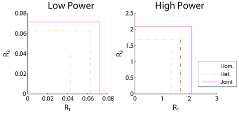
Figure 1: Capacity regions for coherent-state encodings and coherent detection, and achievable rate regions for coherent-state encodings and joint-detection receivers—both with $\eta_{11}=\eta_{22}=1/16$ and $\eta_{12}=\eta_{21}=1/2$ (“very strong” interference for coherent detection and such that (8-9) hold). The LHS displays these regions in a low-power regime with $N_{S_{1}}=N_{S_{2}}=1$ and $N_{B_{1}}=N_{B_{2}}=1$, and the RHS displays these regions in a high-power regime where $N_{S_{1}}=N_{S_{2}}=100$. Homodyne detection outperforms heterodyne detection in the low-power regime because it has a reduced detection noise, while heterodyne detection outperforms homodyne detection in the high-power regime because its has an increased bandwidth.

IV Strong Interference

Sato [12] and Han-Kobayashi [13] independently determined the capacity of a classical Gaussian interference channel under “strong” interference. A channel has “strong” interference if the following information inequalities hold for all $p_{X_{1}}\!\left(x_{1}\right)$ and $p_{X_{2}}\!\left(x_{2}\right)$ [15]:

$$I\left(X_{1};B_{1}|X_{2}\right) \leq I\left(X_{1};B_{2}|X_{2}\right),$$ (10)

$$I\left(X_{2};B_{2}|X_{1}\right) \leq I\left(X_{2};B_{1}|X_{1}\right).$$ (11)

The capacity region of the classical interference channel under this setting is the convex closure of positive rate pairs $\left(R_{1},R_{2}\right)$ such that [12, 13, 15]:

$$R_{1}\leq I\left(X_{1};B_{1}|X_{2}\right),\ \ \ R_{2}\leq I\left(X_{2};B_{2}|X_{1}\right),$$ (12)

$$R_{1}+R_{2}\leq\min\left\{I\left(X_{1}X_{2};B_{1}\right),I\left(X_{1}X_{2};B_{2}\right)\right\}.$$ (13)

The conditions in (10-11) translate to the following ones for coherent-state encoding and coherent detection:

$$\frac{\eta_{21}}{\eta_{22}}\geq\frac{2^{i}\bar{\eta}_{1}N_{B_{1}}+1}{2^{i}\bar{\eta}_{2}N_{B_{2}}+1},\ \ \ \ \ \ \ \ \frac{\eta_{12}}{\eta_{11}}\geq\frac{2^{i}\bar{\eta}_{2}N_{B_{2}}+1}{2^{i}\bar{\eta}_{1}N_{B_{1}}+1},$$

and the capacity region has the two inequalities in (6-7) and an additional bound on the sum rate:

$$R_{1}+R_{2}\leq\frac{1}{2^{i}}\min\left\{\begin{array}[c]{c}\ln\left(1+4^{i}\frac{\eta_{11}N_{S_{1}}+\eta_{21}N_{S_{2}}}{2^{i}\bar{\eta}_{1}N_{B_{1}}+1}\right),\\ \ \ \ \ln\left(1+4^{i}\frac{\eta_{22}N_{S_{2}}+\eta_{12}N_{S_{1}}}{2^{i}\bar{\eta}_{2}N_{B_{2}}+1}\right)\end{array}\right\},$$

where again $i=1$ for homodyne detection and $i=0$ for heterodyne detection.

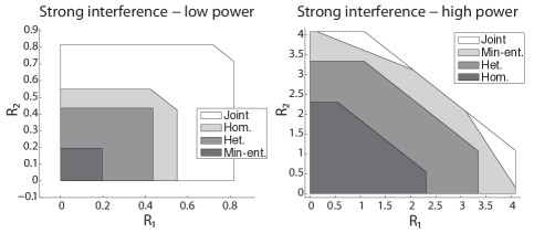
Figure 2: The parameters of the free-space channel are $N_{B_{1}}=N_{B_{2}}=1$, $\eta_{11}=\eta_{22}=0.3$, $\eta_{21}=\eta_{12}=0.6$, $N_{S_{1}}=N_{S_{2}}=2$ for the low-power regime, and $N_{S_{1}}=N_{S_{2}}=100$ for the high-power regime. The LHS figure depicts the “strong” interference capacity regions in the low-power regime for homodyne and heterodyne detection, the achievable rate region with the conjectured joint detection, and the convex hull over regions arising from different min-entropy decoding strategies. Homodyne detection outperforms heterodyne detection in this regime, and the min-entropy decoders perform the worst. The RHS figure displays the same regions in the high-power regime. Heterodyne detection outperforms homodyne detection, and interestingly, the min-entropy decoders outperform heterodyne detection.

The situation for a joint-detection strategy over all of the channel outputs becomes more complicated for the case of “strong” interference, because we require a quantum simultaneous decoder [14] in order to achieve the information rates in (12-13) with $B_{1}$ and $B_{2}$ becoming quantum systems. Such a simultaneous decoder is analogous to a classical simultaneous decoder (e.g., see page 4-15 of Ref. [15]), but we have not yet been able to prove the existence of it in the quantum case (see Conjecture 2 of Ref. [14]). Yet, we do have an achievable simultaneous decoding strategy expressed in terms of min-entropies (see Theorem 4 of Ref. [14]), where the min-entropy of a probability distribution is the negative logarithm of the probability of its mode [17], and, as a simple extension of this idea, the min-entropy of a density operator is the negative logarithm of its maximum eigenvalue. For a thermal state with average photon number $N_{B}$, its min-entropy is $\ln\left(N_{B}+1\right)$, and this result allows us to determine an achievable rate region with a simultaneous decoding strategy (similar to the simultaneous decoding inner bound on page 6-7 of Ref. [15]):

$$R_{1} \leq\ln\left(\eta_{11}N_{S_{1}}+\bar{\eta}_{1}N_{B_{1}}+1\right)-g\left(\bar{\eta}_{1}N_{B_{1}}\right),$$

$$R_{2} \leq\ln\left(\eta_{22}N_{S_{2}}+\bar{\eta}_{2}N_{B_{2}}+1\right)-g\left(\bar{\eta}_{2}N_{B_{2}}\right),$$

$$R_{1}+R_{2}\leq\\ \min\left\{\begin{array}[c]{c}g\left(\eta_{11}N_{S_{1}}+\eta_{21}N_{S_{2}}+\bar{\eta}_{1}N_{B_{1}}\right)-g\left(\bar{\eta}_{1}N_{B_{1}}\right),\\ g\left(\eta_{22}N_{S_{2}}+\eta_{12}N_{S_{1}}+\bar{\eta}_{2}N_{B_{2}}\right)-g\left(\bar{\eta}_{2}N_{B_{2}}\right)\end{array}\right\}.$$

This is one particular variation of an achievable strategy in which we have the bounds on the individual rates expressed in terms of min-entropies and the bound on the sum rate expressed with von Neumann entropies, though note that there are other variations we could consider in light of Theorem 4 of Ref. [14]. We can then take the convex hull of the achievable rate regions for these different strategies to get an achievable rate region for a min-entropy quantum simultaneous decoder (the RHS of Figure 2 displays an interesting example of such a “min-entropy” region). If Conjecture 2 of Ref. [14] regarding the existence of a quantum simultaneous decoder were true, then the rate region in (12-13) would be achievable under under the conditions of (10-11) (with Holevo information rates replacing Shannon rates). Figure 2 displays the different capacity and achievable rate regions when a free-space interference channel exhibits “strong” interference.

V Han-Kobayashi Rate Regions

The Han-Kobayashi region is the best known achievable rate region for the classical interference channel [13]. The coding strategy to achieve this region is for each receiver to decode partially the other sender’s message while fully decoding the partner sender’s message. With this strategy, the four parties can choose to take advantage of channel interference while achieving the task of paired sender-receiver communication.

A compact description of the Han-Kobayashi region comes from its reduction with a Fourier-Motzkin elimination algorithm [18]. It is the convex closure of all positive rate pairs $\left(R_{1},R_{2}\right)$ satisfying the following inequalities and the inequalities obtained from the ones below by swapping the indices 1 and 2:

$$R_{1} \leq I\left(U_{1}W_{1};B_{1}|W_{2}\right),$$ (14)

$$R_{1} \leq I\left(U_{1};B_{1}|W_{1}W_{2}\right)+I\left(W_{1};B_{2}|U_{2}W_{2}\right),$$ (15)

$$R_{1}+R_{2} \leq I\left(U_{1};B_{1}|W_{1}W_{2}\right)+I\left(U_{2}W_{2}W_{1};B_{2}\right),$$ (16)

$$R_{1}+R_{2} \leq I\left(U_{1}W_{2};B_{1}|W_{1}\right)+I\left(U_{2}W_{1};B_{2}|W_{2}\right),$$ (17)

$$2R_{1}+R_{2} \leq I\left(U_{1};B_{1}|W_{1}W_{2}\right)+I\left(U_{1}W_{1}W_{2};B_{1}\right)$$

$$\ \ \ \ \ \ \ \ \ +I\left(U_{2}W_{1};B_{2}|W_{2}\right).$$ (18)

In the above, $U_{m}$ is the “personal” random variable of Sender $m$, and $W_{m}$ is her “common” random variable.

The Han-Kobayashi coding strategy readily translates into a strategy for coherent-state encoding and coherent detection. Sender $m$ shares the total photon number $N_{S_{m}}$ between her personal message and her common message. Let $\lambda_{m}$ be the fraction of signal power that Sender $m$ devotes to her personal message, and let $\bar{\lambda}_{m}$ denote the other fraction of signal power that Sender$~{}m$ devotes to her common message. The inequalities above become the following ones for the case of coherent-state encoding along with coherent detection:

$$R_{1}\leq\gamma\left(\frac{\eta_{11}N_{S_{1}}}{\eta_{21}\lambda_{2}N_{S_{2}}+N_{1}}\right),\ \ \ \ \ \ \ \ \ \ \ \ \ \ \ \ \ \ \ \ \ \ \ \ \ \ \ \ \ \ \ \ \ \$$

$$R_{1}\leq\gamma\left(\frac{\eta_{11}\lambda_{1}N_{S_{1}}}{\eta_{21}\lambda_{2}N_{S_{2}}+N_{1}}\right)+\gamma\left(\frac{\eta_{12}\bar{\lambda}_{1}N_{S_{1}}}{\eta_{12}\lambda_{1}N_{S_{1}}+N_{2}}\right),$$

$$R_{1}+R_{2}\leq\gamma\left(\frac{\eta_{11}\lambda_{1}N_{S_{1}}}{\eta_{21}\lambda_{2}N_{S_{2}}+N_{1}}\right)+\ \ \ \ \ \ \ \ \ \ \ \ \ \ \ \ \ \ \ \ \ \ \ \ \ \ \ \ \ \ \ \ \ \ \ \ \ \ \ \ \ \ \ \$$

$$\gamma\left(\frac{\eta_{12}\bar{\lambda}_{1}N_{S_{1}}+\eta_{22}N_{S_{2}}}{\eta_{12}\lambda_{1}N_{S_{1}}+N_{2}}\right),$$

$$R_{1}+R_{2}\leq\gamma\left(\frac{\eta_{11}\lambda_{1}N_{S_{1}}+\eta_{21}\bar{\lambda}_{2}N_{S_{2}}}{\eta_{21}\lambda_{2}N_{S_{2}}+N_{1}}\right)+\ \ \ \ \ \ \ \ \ \ \ \ \ \ \ \ \ \ \ \ \ \ \ \ \ \ \ \ \ \ \ \ \ \$$

$$\gamma\left(\frac{\eta_{22}\lambda_{2}N_{S_{2}}+\eta_{12}\bar{\lambda}_{1}N_{S_{1}}}{\eta_{12}\lambda_{1}N_{S_{1}}+N_{2}}\right),$$

$$2R_{1}+R_{2}\leq\gamma\left(\frac{\eta_{11}\lambda_{1}N_{S_{1}}}{\eta_{21}\lambda_{2}N_{S_{2}}+N_{1}}\right)+\ \ \ \ \ \ \ \ \ \ \ \ \ \ \ \ \ \ \ \ \ \ \ \ \ \ \ \ \ \ \ \ \ \ \ \ \ \ \ \ \ \ \ \ \ \ \$$

$$\gamma\left(\frac{\eta_{21}\bar{\lambda}_{2}N_{S_{2}}+\eta_{11}N_{S_{1}}}{\eta_{21}\lambda_{2}N_{S_{2}}+N_{1}}\right)+\gamma\left(\frac{\eta_{22}\lambda_{2}N_{S_{2}}+\eta_{12}\bar{\lambda}_{1}N_{S_{1}}}{\eta_{12}\lambda_{1}N_{S_{1}}+N_{2}}\right),$$

where

$$\gamma\left(x\right)=\ln\left(1+x\right)/2^{i},\ \ \ \ N_{m}=\left[2^{i}\bar{\eta}_{m}N_{B_{m}}+1\right]/4^{i},$$

$i=1$ for homodyne detection, $i=0$ for heterodyne detection, and $m\in\left\{1,2\right\}$.

We also conjecture a Han-Kobayashi achievable rate region if the senders employ coherent-state encodings and the receivers exploit joint-detection receivers (this again follows from Conjecture 2 of Ref. [14] regarding the existence of a quantum simultaneous decoder). The inequalities for the region are similar to those in (14-18) and the additional “swapped” inequalities, with the exception that Holevo informations replace mutual informations.

We can obtain an achievable rate region by exploiting the quantum simultaneous decoder from Theorem 4 of Ref. [14] that gives rates which are a difference of a min-entropy and a von Neumann entropy. The region’s characterization is in terms of the Han-Kobayashi (HK) characterization with 14 inequalities [13], corresponding to two different multiple access channels (MACs) induced to each receiver by the HK coding strategy (seven inequalities for each MAC). There are 49 variations of these min-entropy decoders—one of the information rates in the seven inequalities for each MAC is von Neumann and the other six are min-entropy rates. Then taking the convex hull of these 49 different achievable rate regions gives an achievable rate region for a min-entropy decoding strategy. Figure 3 plots the regions achievable with coherent detection, the min-entropy decoder, and the conjectured joint detector for a particular HK power split.

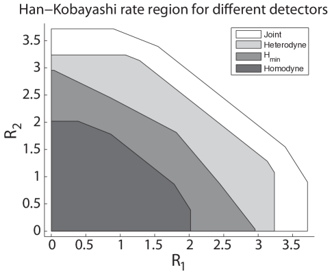
Figure 3: The free-space channel no longer exhibits “very strong” or “strong” interference for coherent detection because the parameters are $N_{S_{1}}=N_{S_{2}}=100$, $N_{B_{1}}=N_{B_{2}}=1$, $\eta_{11}=\eta_{22}=0.8$, and $\eta_{21}=\eta_{12}=0.1$. The figure depicts the achievable rate regions by employing a Han-Kobayashi coding strategy for homodyne and heterodyne detection. It also depicts what we can achieve by employing 49 variations of the min-entropy decoding strategy from Ref. [14] and taking the convex hull of these achievable rate regions. Finally, it displays the conjectured region if a joint detection decoder were to exist (see Conjecture 2 of Ref. [14]). All of these regions are with respect to a 10%-personal, 90%-common Han-Kobayashi power split.

VI Conclusion

The semiclassical models for free-space optical communication are not sufficient to understand the ultimate limits on reliable communication rates, for both point-to-point and multiple-sender-receiver channels. We presented a quantum-mechanical model for the free-space optical interference channel and determined achievable rate regions using both structured and unstructured receivers. Interestingly, the min-entropy decoder from Ref. [14] can achieve rates that are unachievable by both homodyne and heterodyne detection when the channel exhibits “strong interference.”  Finally, we determined the Han-Kobayashi inner bound for homodyne and heterodyne detection, and we conjectured a rate region of this form if a quantum simultaneous decoder were to exist.

Several open problems remain for this line of inquiry. Perhaps the biggest open question is to prove Conjecture 2 from Ref. [14] concerning the existence of a quantum simultaneous decoder for a general quantum interference channel. Also, we do not know if a coherent-state encoding is in fact optimal for the free-space interference channel—it might be that squeezed state transmitters could achieve higher communication rates as in Ref. [6]. One could also evaluate the ergodic and outage capacity regions based on the statistics of $\eta_{ij}$, which could be derived from the spatial coherence functions of the stochastic mode patterns under atmospheric turbulence.

We ackowledge useful discussions with K. Brádler, O. Fawzi, P. Hayden, P. Sen, and B. Yen. S. Guha acknowledges the DARPA Information in a Photon program, contract #HR0011-10-C-0159. M. M. Wilde acknowledges the MDEIE (Québec) PSR-SIIRI international collaboration grant. I. Savov acknowledges support from FQRNT and NSERC.

References

- [1] R. M. Gagliardi and S. Karp, Optical Communications, 2nd ed. John Wiley and Sons, 1995.
- [2] J. H. Shapiro, “The quantum theory of optical communications,” J. Special Topics in Quantum Elect., vol. 15, no. 6, pp. 1547–1569, 2009.
- [3] V. Giovannetti, S. Guha, S. Lloyd, L. Maccone, J. H. Shapiro, and H. P. Yuen, “Classical capacity of the lossy bosonic channel: The exact solution,” Phys. Rev. Lett., vol. 92, no. 2, p. 027902, Jan. 2004.
- [4] S. Guha, “Structured optical receivers to attain superadditive capacity and the Holevo limit,” November 2010, arXiv:1101.1550.
- [5] S. Guha, J. H. Shapiro, and B. I. Erkmen, “Classical capacity of bosonic broadcast communication and a minimum output entropy conjecture,” Physical Review A, vol. 76, p. 032303, 2007.
- [6] B. J. Yen, “Multiple-user quantum optical communication,” Ph.D. dissertation, Massachusetts Institute of Technology, 2005.
- [7] B. Schumacher and M. D. Westmoreland, “Sending classical information via noisy quantum channels,” Phys. Rev. A, vol. 56, pp. 131–138, 1997.
- [8] A. S. Holevo, “The capacity of a quantum channel with general signal states,” IEEE Transactions on Information Theory, vol. 44, p. 269, 1998.
- [9] J. Yard, P. Hayden, and I. Devetak, “Quantum broadcast channels,” 2006, arXiv:quant-ph/0603098.
- [10] ——, “Capacity theorems for quantum multiple-access channels: Classical-quantum and quantum-quantum capacity regions,” IEEE Trans. Inf. Theory, vol. 54, no. 7, pp. 3091–3113, 2008.
- [11] A. B. Carleial, “A case where interference does not reduce capacity,” IEEE Transactions on Information Theory, vol. 21, p. 569, 1975.
- [12] H. Sato, “The capacity of the Gaussian interference channel under strong interference,” IEEE Trans. Inf. Theory, vol. 27, no. 6, pp. 786–788, 1981.
- [13] T.-S. Han and K. Kobayashi, “A new achievable rate region for the interference channel,” IEEE Trans. Inf. Theory, vol. 27, no. 1, pp. 49–60, Jan. 1981.
- [14] O. Fawzi, P. Hayden, I. Savov, P. Sen, and M. M. Wilde, “Classical communication over a quantum interference channel,” 2011.
- [15] A. El Gamal and Y. H. Kim, “Lecture notes on network information theory,” January 2010, arXiv:1001.3404.
- [16] V. Giovannetti, A. S. Holevo, S. Lloyd, and L. Maccone, “Generalized minimal output entropy conjecture for one-mode Gaussian channels: definitions and some exact results,” Journal of Physics A: Mathematical and Theoretical, vol. 43, no. 41, p. 415305, 2010.
- [17] A. Rényi, “On measures of information and entropy,” Proc. of the 4th Berkeley Symp. on Math., Stat., and Prob., pp. 547–561, 1960.
- [18] H.-F. Chong, M. Motani, H. K. Garg, and H. El Gamal, “On the Han-Kobayashi region for the interference channel,” IEEE Transactions on Information Theory, vol. 54, no. 7, pp. 3188–3195, 2008.