STAR Collaboration

High $p_{T}$ non-photonic electron production in $p$ + $p$ collisions at $\sqrt{s}$ = 200 GeV

H. Agakishiev Joint Institute for Nuclear Research, Dubna, 141 980, Russia M. M. Aggarwal Panjab University, Chandigarh 160014, India Z. Ahammed Lawrence Berkeley National Laboratory, Berkeley, California 94720, USA A. V. Alakhverdyants Joint Institute for Nuclear Research, Dubna, 141 980, Russia I. Alekseev Alikhanov Institute for Theoretical and Experimental Physics, Moscow, Russia J. Alford Kent State University, Kent, Ohio 44242, USA B. D. Anderson Kent State University, Kent, Ohio 44242, USA C. D. Anson Ohio State University, Columbus, Ohio 43210, USA D. Arkhipkin Brookhaven National Laboratory, Upton, New York 11973, USA G. S. Averichev Joint Institute for Nuclear Research, Dubna, 141 980, Russia J. Balewski Massachusetts Institute of Technology, Cambridge, MA 02139-4307, USA D. R. Beavis Brookhaven National Laboratory, Upton, New York 11973, USA N. K. Behera Indian Institute of Technology, Mumbai, India R. Bellwied University of Houston, Houston, TX, 77204, USA M. J. Betancourt Massachusetts Institute of Technology, Cambridge, MA 02139-4307, USA R. R. Betts University of Illinois at Chicago, Chicago, Illinois 60607, USA A. Bhasin University of Jammu, Jammu 180001, India A. K. Bhati Panjab University, Chandigarh 160014, India H. Bichsel University of Washington, Seattle, Washington 98195, USA J. Bielcik Czech Technical University in Prague, FNSPE, Prague, 115 19, Czech Republic J. Bielcikova Nuclear Physics Institute AS CR, 250 68 Řež/Prague, Czech Republic B. Biritz University of California, Los Angeles, California 90095, USA L. C. Bland Brookhaven National Laboratory, Upton, New York 11973, USA I. G. Bordyuzhin Alikhanov Institute for Theoretical and Experimental Physics, Moscow, Russia W. Borowski SUBATECH, Nantes, France J. Bouchet Kent State University, Kent, Ohio 44242, USA E. Braidot NIKHEF and Utrecht University, Amsterdam, The Netherlands A. V. Brandin Moscow Engineering Physics Institute, Moscow Russia A. Bridgeman Argonne National Laboratory, Argonne, Illinois 60439, USA S. G. Brovko University of California, Davis, California 95616, USA E. Bruna Yale University, New Haven, Connecticut 06520, USA S. Bueltmann Old Dominion University, Norfolk, VA, 23529, USA I. Bunzarov Joint Institute for Nuclear Research, Dubna, 141 980, Russia T. P. Burton Brookhaven National Laboratory, Upton, New York 11973, USA X. Z. Cai Shanghai Institute of Applied Physics, Shanghai 201800, China H. Caines Yale University, New Haven, Connecticut 06520, USA M. Calderón de la Barca Sánchez University of California, Davis, California 95616, USA D. Cebra University of California, Davis, California 95616, USA R. Cendejas University of California, Los Angeles, California 90095, USA M. C. Cervantes Texas A&M University, College Station, Texas 77843, USA Z. Chajecki Ohio State University, Columbus, Ohio 43210, USA P. Chaloupka Nuclear Physics Institute AS CR, 250 68 Řež/Prague, Czech Republic S. Chattopadhyay Variable Energy Cyclotron Centre, Kolkata 700064, India H. F. Chen University of Science & Technology of China, Hefei 230026, China J. H. Chen Shanghai Institute of Applied Physics, Shanghai 201800, China J. Y. Chen Institute of Particle Physics, CCNU (HZNU), Wuhan 430079, China L. Chen Institute of Particle Physics, CCNU (HZNU), Wuhan 430079, China J. Cheng Tsinghua University, Beijing 100084, China M. Cherney Creighton University, Omaha, Nebraska 68178, USA A. Chikanian Yale University, New Haven, Connecticut 06520, USA K. E. Choi Pusan National University, Pusan, Republic of Korea W. Christie Brookhaven National Laboratory, Upton, New York 11973, USA P. Chung Nuclear Physics Institute AS CR, 250 68 Řež/Prague, Czech Republic M. J. M. Codrington Texas A&M University, College Station, Texas 77843, USA R. Corliss Massachusetts Institute of Technology, Cambridge, MA 02139-4307, USA J. G. Cramer University of Washington, Seattle, Washington 98195, USA H. J. Crawford University of California, Berkeley, California 94720, USA S. Dash Institute of Physics, Bhubaneswar 751005, India A. Davila Leyva University of Texas, Austin, Texas 78712, USA L. C. De Silva University of Houston, Houston, TX, 77204, USA R. R. Debbe Brookhaven National Laboratory, Upton, New York 11973, USA T. G. Dedovich Joint Institute for Nuclear Research, Dubna, 141 980, Russia A. A. Derevschikov Institute of High Energy Physics, Protvino, Russia R. Derradi de Souza Universidade Estadual de Campinas, Sao Paulo, Brazil L. Didenko Brookhaven National Laboratory, Upton, New York 11973, USA P. Djawotho Texas A&M University, College Station, Texas 77843, USA S. M. Dogra University of Jammu, Jammu 180001, India X. Dong Lawrence Berkeley National Laboratory, Berkeley, California 94720, USA J. L. Drachenberg Texas A&M University, College Station, Texas 77843, USA J. E. Draper University of California, Davis, California 95616, USA J. C. Dunlop Brookhaven National Laboratory, Upton, New York 11973, USA L. G. Efimov Joint Institute for Nuclear Research, Dubna, 141 980, Russia M. Elnimr Wayne State University, Detroit, Michigan 48201, USA J. Engelage University of California, Berkeley, California 94720, USA G. Eppley Rice University, Houston, Texas 77251, USA M. Estienne SUBATECH, Nantes, France L. Eun Pennsylvania State University, University Park, Pennsylvania 16802, USA O. Evdokimov University of Illinois at Chicago, Chicago, Illinois 60607, USA R. Fatemi University of Kentucky, Lexington, Kentucky, 40506-0055, USA J. Fedorisin Joint Institute for Nuclear Research, Dubna, 141 980, Russia R. G. Fersch University of Kentucky, Lexington, Kentucky, 40506-0055, USA P. Filip Joint Institute for Nuclear Research, Dubna, 141 980, Russia E. Finch Yale University, New Haven, Connecticut 06520, USA V. Fine Brookhaven National Laboratory, Upton, New York 11973, USA Y. Fisyak Brookhaven National Laboratory, Upton, New York 11973, USA C. A. Gagliardi Texas A&M University, College Station, Texas 77843, USA D. R. Gangadharan University of California, Los Angeles, California 90095, USA A. Geromitsos SUBATECH, Nantes, France F. Geurts Rice University, Houston, Texas 77251, USA P. Ghosh Variable Energy Cyclotron Centre, Kolkata 700064, India Y. N. Gorbunov Creighton University, Omaha, Nebraska 68178, USA A. Gordon Brookhaven National Laboratory, Upton, New York 11973, USA O. G. Grebenyuk Lawrence Berkeley National Laboratory, Berkeley, California 94720, USA D. Grosnick Valparaiso University, Valparaiso, Indiana 46383, USA S. M. Guertin University of California, Los Angeles, California 90095, USA A. Gupta University of Jammu, Jammu 180001, India W. Guryn Brookhaven National Laboratory, Upton, New York 11973, USA B. Haag University of California, Davis, California 95616, USA O. Hajkova Czech Technical University in Prague, FNSPE, Prague, 115 19, Czech Republic A. Hamed Texas A&M University, College Station, Texas 77843, USA L-X. Han Shanghai Institute of Applied Physics, Shanghai 201800, China J. W. Harris Yale University, New Haven, Connecticut 06520, USA J. P. Hays-Wehle Massachusetts Institute of Technology, Cambridge, MA 02139-4307, USA M. Heinz Yale University, New Haven, Connecticut 06520, USA S. Heppelmann Pennsylvania State University, University Park, Pennsylvania 16802, USA A. Hirsch Purdue University, West Lafayette, Indiana 47907, USA E. Hjort Lawrence Berkeley National Laboratory, Berkeley, California 94720, USA G. W. Hoffmann University of Texas, Austin, Texas 78712, USA D. J. Hofman University of Illinois at Chicago, Chicago, Illinois 60607, USA B. Huang University of Science & Technology of China, Hefei 230026, China H. Z. Huang University of California, Los Angeles, California 90095, USA T. J. Humanic Ohio State University, Columbus, Ohio 43210, USA L. Huo Texas A&M University, College Station, Texas 77843, USA G. Igo University of California, Los Angeles, California 90095, USA P. Jacobs Lawrence Berkeley National Laboratory, Berkeley, California 94720, USA W. W. Jacobs Indiana University, Bloomington, Indiana 47408, USA C. Jena Institute of Physics, Bhubaneswar 751005, India F. Jin Shanghai Institute of Applied Physics, Shanghai 201800, China J. Joseph Kent State University, Kent, Ohio 44242, USA E. G. Judd University of California, Berkeley, California 94720, USA S. Kabana SUBATECH, Nantes, France K. Kang Tsinghua University, Beijing 100084, China J. Kapitan Nuclear Physics Institute AS CR, 250 68 Řež/Prague, Czech Republic K. Kauder University of Illinois at Chicago, Chicago, Illinois 60607, USA H. W. Ke Institute of Particle Physics, CCNU (HZNU), Wuhan 430079, China D. Keane Kent State University, Kent, Ohio 44242, USA A. Kechechyan Joint Institute for Nuclear Research, Dubna, 141 980, Russia D. Kettler University of Washington, Seattle, Washington 98195, USA D. P. Kikola Lawrence Berkeley National Laboratory, Berkeley, California 94720, USA J. Kiryluk Lawrence Berkeley National Laboratory, Berkeley, California 94720, USA A. Kisiel Warsaw University of Technology, Warsaw, Poland V. Kizka Joint Institute for Nuclear Research, Dubna, 141 980, Russia S. R. Klein Lawrence Berkeley National Laboratory, Berkeley, California 94720, USA A. G. Knospe Yale University, New Haven, Connecticut 06520, USA D. D. Koetke Valparaiso University, Valparaiso, Indiana 46383, USA T. Kollegger University of Frankfurt, Frankfurt, Germany J. Konzer Purdue University, West Lafayette, Indiana 47907, USA I. Koralt Old Dominion University, Norfolk, VA, 23529, USA L. Koroleva Alikhanov Institute for Theoretical and Experimental Physics, Moscow, Russia W. Korsch University of Kentucky, Lexington, Kentucky, 40506-0055, USA L. Kotchenda Moscow Engineering Physics Institute, Moscow Russia V. Kouchpil Nuclear Physics Institute AS CR, 250 68 Řež/Prague, Czech Republic P. Kravtsov Moscow Engineering Physics Institute, Moscow Russia K. Krueger Argonne National Laboratory, Argonne, Illinois 60439, USA M. Krus Czech Technical University in Prague, FNSPE, Prague, 115 19, Czech Republic L. Kumar Kent State University, Kent, Ohio 44242, USA P. Kurnadi University of California, Los Angeles, California 90095, USA M. A. C. Lamont Brookhaven National Laboratory, Upton, New York 11973, USA J. M. Landgraf Brookhaven National Laboratory, Upton, New York 11973, USA S. LaPointe Wayne State University, Detroit, Michigan 48201, USA J. Lauret Brookhaven National Laboratory, Upton, New York 11973, USA A. Lebedev Brookhaven National Laboratory, Upton, New York 11973, USA R. Lednicky Joint Institute for Nuclear Research, Dubna, 141 980, Russia J. H. Lee Brookhaven National Laboratory, Upton, New York 11973, USA W. Leight Massachusetts Institute of Technology, Cambridge, MA 02139-4307, USA M. J. LeVine Brookhaven National Laboratory, Upton, New York 11973, USA C. Li University of Science & Technology of China, Hefei 230026, China L. Li University of Texas, Austin, Texas 78712, USA N. Li Institute of Particle Physics, CCNU (HZNU), Wuhan 430079, China W. Li Shanghai Institute of Applied Physics, Shanghai 201800, China X. Li Purdue University, West Lafayette, Indiana 47907, USA X. Li Shandong University, Jinan, Shandong 250100, China Y. Li Tsinghua University, Beijing 100084, China Z. M. Li Institute of Particle Physics, CCNU (HZNU), Wuhan 430079, China M. A. Lisa Ohio State University, Columbus, Ohio 43210, USA F. Liu Institute of Particle Physics, CCNU (HZNU), Wuhan 430079, China H. Liu University of California, Davis, California 95616, USA J. Liu Rice University, Houston, Texas 77251, USA T. Ljubicic Brookhaven National Laboratory, Upton, New York 11973, USA W. J. Llope Rice University, Houston, Texas 77251, USA R. S. Longacre Brookhaven National Laboratory, Upton, New York 11973, USA W. A. Love Brookhaven National Laboratory, Upton, New York 11973, USA Y. Lu University of Science & Technology of China, Hefei 230026, China E. V. Lukashov Moscow Engineering Physics Institute, Moscow Russia X. Luo University of Science & Technology of China, Hefei 230026, China G. L. Ma Shanghai Institute of Applied Physics, Shanghai 201800, China Y. G. Ma Shanghai Institute of Applied Physics, Shanghai 201800, China D. P. Mahapatra Institute of Physics, Bhubaneswar 751005, India R. Majka Yale University, New Haven, Connecticut 06520, USA O. I. Mall University of California, Davis, California 95616, USA L. K. Mangotra University of Jammu, Jammu 180001, India R. Manweiler Valparaiso University, Valparaiso, Indiana 46383, USA S. Margetis Kent State University, Kent, Ohio 44242, USA C. Markert University of Texas, Austin, Texas 78712, USA H. Masui Lawrence Berkeley National Laboratory, Berkeley, California 94720, USA H. S. Matis Lawrence Berkeley National Laboratory, Berkeley, California 94720, USA Yu. A. Matulenko Institute of High Energy Physics, Protvino, Russia D. McDonald Rice University, Houston, Texas 77251, USA T. S. McShane Creighton University, Omaha, Nebraska 68178, USA A. Meschanin Institute of High Energy Physics, Protvino, Russia R. Milner Massachusetts Institute of Technology, Cambridge, MA 02139-4307, USA N. G. Minaev Institute of High Energy Physics, Protvino, Russia S. Mioduszewski Texas A&M University, College Station, Texas 77843, USA A. Mischke NIKHEF and Utrecht University, Amsterdam, The Netherlands M. K. Mitrovski University of Frankfurt, Frankfurt, Germany Y. Mohammed Texas A&M University, College Station, Texas 77843, USA B. Mohanty Variable Energy Cyclotron Centre, Kolkata 700064, India M. M. Mondal Variable Energy Cyclotron Centre, Kolkata 700064, India B. Morozov Alikhanov Institute for Theoretical and Experimental Physics, Moscow, Russia D. A. Morozov Institute of High Energy Physics, Protvino, Russia M. G. Munhoz Universidade de Sao Paulo, Sao Paulo, Brazil M. K. Mustafa Purdue University, West Lafayette, Indiana 47907, USA M. Naglis Lawrence Berkeley National Laboratory, Berkeley, California 94720, USA B. K. Nandi Indian Institute of Technology, Mumbai, India T. K. Nayak Variable Energy Cyclotron Centre, Kolkata 700064, India P. K. Netrakanti Purdue University, West Lafayette, Indiana 47907, USA L. V. Nogach Institute of High Energy Physics, Protvino, Russia S. B. Nurushev Institute of High Energy Physics, Protvino, Russia G. Odyniec Lawrence Berkeley National Laboratory, Berkeley, California 94720, USA A. Ogawa Brookhaven National Laboratory, Upton, New York 11973, USA K. Oh Pusan National University, Pusan, Republic of Korea A. Ohlson Yale University, New Haven, Connecticut 06520, USA V. Okorokov Moscow Engineering Physics Institute, Moscow Russia E. W. Oldag University of Texas, Austin, Texas 78712, USA D. Olson Lawrence Berkeley National Laboratory, Berkeley, California 94720, USA M. Pachr Czech Technical University in Prague, FNSPE, Prague, 115 19, Czech Republic B. S. Page Indiana University, Bloomington, Indiana 47408, USA S. K. Pal Variable Energy Cyclotron Centre, Kolkata 700064, India Y. Pandit Kent State University, Kent, Ohio 44242, USA Y. Panebratsev Joint Institute for Nuclear Research, Dubna, 141 980, Russia T. Pawlak Warsaw University of Technology, Warsaw, Poland H. Pei University of Illinois at Chicago, Chicago, Illinois 60607, USA T. Peitzmann NIKHEF and Utrecht University, Amsterdam, The Netherlands C. Perkins University of California, Berkeley, California 94720, USA W. Peryt Warsaw University of Technology, Warsaw, Poland S. C. Phatak Institute of Physics, Bhubaneswar 751005, India P. Pile Brookhaven National Laboratory, Upton, New York 11973, USA M. Planinic University of Zagreb, Zagreb, HR-10002, Croatia M. A. Ploskon Lawrence Berkeley National Laboratory, Berkeley, California 94720, USA J. Pluta Warsaw University of Technology, Warsaw, Poland D. Plyku Old Dominion University, Norfolk, VA, 23529, USA N. Poljak University of Zagreb, Zagreb, HR-10002, Croatia A. M. Poskanzer Lawrence Berkeley National Laboratory, Berkeley, California 94720, USA B. V. K. S. Potukuchi University of Jammu, Jammu 180001, India C. B. Powell Lawrence Berkeley National Laboratory, Berkeley, California 94720, USA D. Prindle University of Washington, Seattle, Washington 98195, USA C. Pruneau Wayne State University, Detroit, Michigan 48201, USA N. K. Pruthi Panjab University, Chandigarh 160014, India P. R. Pujahari Indian Institute of Technology, Mumbai, India J. Putschke Yale University, New Haven, Connecticut 06520, USA H. Qiu Institute of Modern Physics, Lanzhou, China R. Raniwala University of Rajasthan, Jaipur 302004, India S. Raniwala University of Rajasthan, Jaipur 302004, India R. L. Ray University of Texas, Austin, Texas 78712, USA R. Redwine Massachusetts Institute of Technology, Cambridge, MA 02139-4307, USA R. Reed University of California, Davis, California 95616, USA H. G. Ritter Lawrence Berkeley National Laboratory, Berkeley, California 94720, USA J. B. Roberts Rice University, Houston, Texas 77251, USA O. V. Rogachevskiy Joint Institute for Nuclear Research, Dubna, 141 980, Russia J. L. Romero University of California, Davis, California 95616, USA A. Rose Lawrence Berkeley National Laboratory, Berkeley, California 94720, USA L. Ruan Brookhaven National Laboratory, Upton, New York 11973, USA J. Rusnak Nuclear Physics Institute AS CR, 250 68 Řež/Prague, Czech Republic N. R. Sahoo Variable Energy Cyclotron Centre, Kolkata 700064, India S. Sakai Lawrence Berkeley National Laboratory, Berkeley, California 94720, USA I. Sakrejda Lawrence Berkeley National Laboratory, Berkeley, California 94720, USA S. Salur University of California, Davis, California 95616, USA J. Sandweiss Yale University, New Haven, Connecticut 06520, USA E. Sangaline University of California, Davis, California 95616, USA A. Sarkar Indian Institute of Technology, Mumbai, India J. Schambach University of Texas, Austin, Texas 78712, USA R. P. Scharenberg Purdue University, West Lafayette, Indiana 47907, USA A. M. Schmah Lawrence Berkeley National Laboratory, Berkeley, California 94720, USA N. Schmitz Max-Planck-Institut für Physik, Munich, Germany T. R. Schuster University of Frankfurt, Frankfurt, Germany J. Seele Massachusetts Institute of Technology, Cambridge, MA 02139-4307, USA J. Seger Creighton University, Omaha, Nebraska 68178, USA I. Selyuzhenkov Indiana University, Bloomington, Indiana 47408, USA P. Seyboth Max-Planck-Institut für Physik, Munich, Germany E. Shahaliev Joint Institute for Nuclear Research, Dubna, 141 980, Russia M. Shao University of Science & Technology of China, Hefei 230026, China M. Sharma Wayne State University, Detroit, Michigan 48201, USA S. S. Shi Institute of Particle Physics, CCNU (HZNU), Wuhan 430079, China Q. Y. Shou Shanghai Institute of Applied Physics, Shanghai 201800, China E. P. Sichtermann Lawrence Berkeley National Laboratory, Berkeley, California 94720, USA F. Simon Max-Planck-Institut für Physik, Munich, Germany R. N. Singaraju Variable Energy Cyclotron Centre, Kolkata 700064, India M. J. Skoby Purdue University, West Lafayette, Indiana 47907, USA N. Smirnov Yale University, New Haven, Connecticut 06520, USA P. Sorensen Brookhaven National Laboratory, Upton, New York 11973, USA H. M. Spinka Argonne National Laboratory, Argonne, Illinois 60439, USA B. Srivastava Purdue University, West Lafayette, Indiana 47907, USA T. D. S. Stanislaus Valparaiso University, Valparaiso, Indiana 46383, USA D. Staszak University of California, Los Angeles, California 90095, USA S. G. Steadman Massachusetts Institute of Technology, Cambridge, MA 02139-4307, USA J. R. Stevens Indiana University, Bloomington, Indiana 47408, USA R. Stock University of Frankfurt, Frankfurt, Germany M. Strikhanov Moscow Engineering Physics Institute, Moscow Russia B. Stringfellow Purdue University, West Lafayette, Indiana 47907, USA A. A. P. Suaide Universidade de Sao Paulo, Sao Paulo, Brazil M. C. Suarez University of Illinois at Chicago, Chicago, Illinois 60607, USA N. L. Subba Kent State University, Kent, Ohio 44242, USA M. Sumbera Nuclear Physics Institute AS CR, 250 68 Řež/Prague, Czech Republic X. M. Sun Lawrence Berkeley National Laboratory, Berkeley, California 94720, USA Y. Sun University of Science & Technology of China, Hefei 230026, China Z. Sun Institute of Modern Physics, Lanzhou, China B. Surrow Massachusetts Institute of Technology, Cambridge, MA 02139-4307, USA D. N. Svirida Alikhanov Institute for Theoretical and Experimental Physics, Moscow, Russia T. J. M. Symons Lawrence Berkeley National Laboratory, Berkeley, California 94720, USA A. Szanto de Toledo Universidade de Sao Paulo, Sao Paulo, Brazil J. Takahashi Universidade Estadual de Campinas, Sao Paulo, Brazil A. H. Tang Brookhaven National Laboratory, Upton, New York 11973, USA Z. Tang University of Science & Technology of China, Hefei 230026, China L. H. Tarini Wayne State University, Detroit, Michigan 48201, USA T. Tarnowsky Michigan State University, East Lansing, Michigan 48824, USA D. Thein University of Texas, Austin, Texas 78712, USA J. H. Thomas Lawrence Berkeley National Laboratory, Berkeley, California 94720, USA J. Tian Shanghai Institute of Applied Physics, Shanghai 201800, China A. R. Timmins University of Houston, Houston, TX, 77204, USA D. Tlusty Nuclear Physics Institute AS CR, 250 68 Řež/Prague, Czech Republic M. Tokarev Joint Institute for Nuclear Research, Dubna, 141 980, Russia T. A. Trainor University of Washington, Seattle, Washington 98195, USA V. N. Tram Lawrence Berkeley National Laboratory, Berkeley, California 94720, USA S. Trentalange University of California, Los Angeles, California 90095, USA R. E. Tribble Texas A&M University, College Station, Texas 77843, USA P. Tribedy Variable Energy Cyclotron Centre, Kolkata 700064, India O. D. Tsai University of California, Los Angeles, California 90095, USA T. Ullrich Brookhaven National Laboratory, Upton, New York 11973, USA D. G. Underwood Argonne National Laboratory, Argonne, Illinois 60439, USA G. Van Buren Brookhaven National Laboratory, Upton, New York 11973, USA G. van Nieuwenhuizen Massachusetts Institute of Technology, Cambridge, MA 02139-4307, USA J. A. Vanfossen, Jr Kent State University, Kent, Ohio 44242, USA R. Varma Indian Institute of Technology, Mumbai, India G. M. S. Vasconcelos Universidade Estadual de Campinas, Sao Paulo, Brazil A. N. Vasiliev Institute of High Energy Physics, Protvino, Russia F. Videbæk Brookhaven National Laboratory, Upton, New York 11973, USA Y. P. Viyogi Variable Energy Cyclotron Centre, Kolkata 700064, India S. Vokal Joint Institute for Nuclear Research, Dubna, 141 980, Russia S. A. Voloshin Wayne State University, Detroit, Michigan 48201, USA M. Wada University of Texas, Austin, Texas 78712, USA M. Walker Massachusetts Institute of Technology, Cambridge, MA 02139-4307, USA F. Wang Purdue University, West Lafayette, Indiana 47907, USA G. Wang University of California, Los Angeles, California 90095, USA H. Wang Michigan State University, East Lansing, Michigan 48824, USA J. S. Wang Institute of Modern Physics, Lanzhou, China Q. Wang Purdue University, West Lafayette, Indiana 47907, USA X. L. Wang University of Science & Technology of China, Hefei 230026, China Y. Wang Tsinghua University, Beijing 100084, China G. Webb University of Kentucky, Lexington, Kentucky, 40506-0055, USA J. C. Webb Brookhaven National Laboratory, Upton, New York 11973, USA G. D. Westfall Michigan State University, East Lansing, Michigan 48824, USA C. Whitten Jr University of California, Los Angeles, California 90095, USA H. Wieman Lawrence Berkeley National Laboratory, Berkeley, California 94720, USA S. W. Wissink Indiana University, Bloomington, Indiana 47408, USA R. Witt United States Naval Academy, Annapolis, MD 21402, USA W. Witzke University of Kentucky, Lexington, Kentucky, 40506-0055, USA Y. F. Wu Institute of Particle Physics, CCNU (HZNU), Wuhan 430079, China Z. Xiao Tsinghua University, Beijing 100084, China W. Xie Purdue University, West Lafayette, Indiana 47907, USA H. Xu Institute of Modern Physics, Lanzhou, China N. Xu Lawrence Berkeley National Laboratory, Berkeley, California 94720, USA Q. H. Xu Shandong University, Jinan, Shandong 250100, China W. Xu University of California, Los Angeles, California 90095, USA Y. Xu University of Science & Technology of China, Hefei 230026, China Z. Xu Brookhaven National Laboratory, Upton, New York 11973, USA L. Xue Shanghai Institute of Applied Physics, Shanghai 201800, China Y. Yang Institute of Modern Physics, Lanzhou, China Y. Yang Institute of Particle Physics, CCNU (HZNU), Wuhan 430079, China P. Yepes Rice University, Houston, Texas 77251, USA K. Yip Brookhaven National Laboratory, Upton, New York 11973, USA I-K. Yoo Pusan National University, Pusan, Republic of Korea M. Zawisza Warsaw University of Technology, Warsaw, Poland H. Zbroszczyk Warsaw University of Technology, Warsaw, Poland W. Zhan Institute of Modern Physics, Lanzhou, China J. B. Zhang Institute of Particle Physics, CCNU (HZNU), Wuhan 430079, China S. Zhang Shanghai Institute of Applied Physics, Shanghai 201800, China W. M. Zhang Kent State University, Kent, Ohio 44242, USA X. P. Zhang Tsinghua University, Beijing 100084, China Y. Zhang Lawrence Berkeley National Laboratory, Berkeley, California 94720, USA Z. P. Zhang University of Science & Technology of China, Hefei 230026, China J. Zhao Shanghai Institute of Applied Physics, Shanghai 201800, China C. Zhong Shanghai Institute of Applied Physics, Shanghai 201800, China W. Zhou Shandong University, Jinan, Shandong 250100, China X. Zhu Tsinghua University, Beijing 100084, China Y. H. Zhu Shanghai Institute of Applied Physics, Shanghai 201800, China R. Zoulkarneev Joint Institute for Nuclear Research, Dubna, 141 980, Russia Y. Zoulkarneeva Joint Institute for Nuclear Research, Dubna, 141 980, Russia

Abstract

We present the measurement of non-photonic electron production at high transverse momentum ( $p_{T}>$ 2.5 GeV/ $c$ ) in $p$ + $p$ collisions at $\sqrt{s}$ = 200 GeV using data recorded during 2005 and 2008 by the STAR experiment at the Relativistic Heavy Ion Collider (RHIC). The measured cross-sections from the two runs are consistent with each other despite a large difference in photonic background levels due to different detector configurations. We compare the measured non-photonic electron cross-sections with previously published RHIC data and pQCD calculations. Using the relative contributions of B and D mesons to non-photonic electrons, we determine the integrated cross sections of electrons ( $\frac{e^{+}+e^{-}}{2}$ ) at 3 GeV/ $c<p_{T}<~{}$ 10 GeV/ $c$ from bottom and charm meson decays to be ${d\sigma_{(B\to e)+(B\to D\to e)}\over dy_{e}}|_{y_{e}=0}$ = 4.0 $\pm 0.5$ (stat.) $\pm 1.1$ (syst.) nb and ${d\sigma_{D\to e}\over dy_{e}}|_{y_{e}=0}$ = 6.2 $\pm 0.7$ (stat.) $\pm 1.5$ (syst.) nb, respectively.

pacs:

13.20.Fc, 13.20.He, 25.75.Cj

I Introduction

Heavy quark production in high-energy hadronic collisions has been a focus of interest for years. It is one of the few instances in which experimental measurements can be compared with QCD predictions over nearly the entire kinematical range Cacciari:2007hn ; Cacciari:2005rk ; Frixione:2005yf . Due to the large masses of charm and bottom quarks, they are produced almost exclusively during the initial high-Q parton-parton interactions and thus can be described by perturbative QCD calculations.

Measurement of heavy flavor production in elementary collisions represents a crucial test of the validity of the current theoretical framework and its phenomenological inputs. It is also mandatory as a baseline for the interpretation of heavy flavor production in nucleus-nucleus collisions Frawley:2008kk . In these heavy-ion collisions one investigates the properties of the quark-gluon plasma (QGP), which is created at sufficiently high center-of-mass energies. Many effects on heavy flavor production in heavy-ion collisions have been observed but are quantitatively not yet fully understood Frawley:2008kk . Of particular interest are effects which modify the transverse momentum spectra of heavy flavor hadrons, including energy loss in the QGP (”jet quenching”) Mustafa:1997pm ; Djordjevic:2005db ; Wicks:2005gt ; Djordjevic:2008iz ; Sharma:2009hn , as well as collective effects such as elliptic flow Moore:2004tg ; vanHees:2005wb . In addition, $J/\psi$ might be regenerated in a dense plasma from the initial open charm yield Grandchamp:2002iy , making precise measurements of the transverse momentum spectra in elementary $p$ + $p$ collisions imperative.

Open heavy-flavor production in p+p, d+A, and A+A collisions at $\sqrt{s_{NN}}$ = 200 GeV has been studied at the Relativistic Heavy Ion Collider (RHIC) using a variety of final-state observables Frawley:2008kk . The STAR collaboration measured charm mesons directly through their hadronic decay channels Dstar:2009df ; Adams:2004fc ; Baumgart:2008zz . Due to the lack of precise secondary vertex tracking and trigger capabilities these measurements are restricted to low momenta ( $\mbox{$p_{T}$}<3$ GeV/ $c$ ). Both STAR Adams:2004fc ; Abelev:2006db and PHENIX Adler:2005xv ; Adare:2006hc also measured heavy flavor production through semileptonic decays of charm and bottom mesons ( $D,B\rightarrow\ell\ \nu_{\ell}\ X$ ). While the measured decay leptons provide only limited information on the original kinematics of the heavy flavor parton, these measurements are facilitated by fast online triggers and extend the kinematic range to high $p_{T}$ .

In this paper, we report STAR results on non-photonic electron production at midrapidity in p+p collisions at $\sqrt{s}$ = 200 GeV using data recorded during year 2005 (Run2005) and year 2008 (Run2008) with a total integrated luminosity of 2.8 pb^-1 and 2.6 pb^-1, respectively. The present results are consistent with the Next-to-Leading Logarithm (FONLL) calculation within its theoretical uncertainties. Utilizing the measured relative contributions of B and D mesons to non-photonic electrons which were obtained from a study of electron-hadron correlations (e-h) e_h , we determine the invariant cross section of electrons from bottom and charm meson decays separately at $p_{T}>$ 3.0 GeV/ $c$ .

The article is organized as follows. In Sec. II we describe the STAR detectors and triggers relevant to this analysis. Sec. III describes the data analysis in detail, and in Sec. IV we present and discuss the results. Sec. V provides conclusions.

II Experiment

II.1 Detectors

STAR is a large acceptance, multi-purpose experiment composed of several individual detector subsystems with tracking inside a large solenoidal magnet generating a uniform field of 0.5 T Ackermann:2002ad . The detector subsystems relevant for the present analysis are briefly described in the following.

II.1.1 Time Projection Chamber

The Time Projection Chamber (TPC) tpc is the main charged particle tracking device in STAR. The TPC covers $\pm$ 1.0 units in pseudorapidity ( $\eta$ ) for tracks crossing all layers of pads, and the full azimuth. Particle momentum is determined from track curvature in the solenoidal field. In this analysis, TPC tracks are used for momentum determination, electron-hadron separation (using specific ionization $dE/dx$ ), to reconstruct the interaction vertex, and to project to the calorimeter for further hadron rejection.

II.1.2 Barrel Electromagnetic Calorimeter and
Barrel Shower Maximum Detector

The Barrel Electromagnetic Calorimeter (BEMC) measures the energy deposited by photons and electrons and provides a trigger signal. It is located inside the magnet coil outside the TPC, covering $|\eta|<1.0$ and $2\pi$ in azimuth, matching the TPC acceptance. The BEMC is a lead-scintillator sampling electromagnetic calorimeter with a nominal energy resolution of $\delta E/E\sim 14\%/\sqrt{E/1{\rm GeV}}\oplus 1.5\%$ bemc . The full calorimeter is segmented into 4800 projective towers. A tower covers 0.05 rad in $\phi$ and 0.05 units in $\eta$ . Each tower consists of a stack of 20 layers of lead and 21 layers of scintillator with an active depth of 23.5 cm. The first two scintillator layers are read out separately providing the calorimeter preshower signal, which is not used in this analysis. A Shower Maximum Detector (BSMD) is positioned behind the fifth scintillator layer. The BSMD is a double layer wire proportional counter with strip readout. The two layers of the BSMD, each containing 18000 strips, provide precise spacial resolution in $\phi$ and $\eta$ and improve the electron-hadron separation. The BEMC also provides a high-energy trigger based on the highest energy measured by a single tower in order to enrich the event samples with high- $p_{T}$ electromagnetic energy deposition.

II.1.3 Trigger Detectors

The Beam-Beam Counters (BBC) bbc are two identical counters located on each side of the interaction region covering the full azimuth and 2.1 $<|\eta|<$ 5.0. Each detector consists of sets of small and large hexagonal scintillator tiles grouped into a ring and mounted around the beam pipe at a distance of 3.7 m from the interaction point. In both Run2008 and Run2005, the BBC served as a minimum-bias trigger to record the integrated luminosity by requiring a coincidence of signals in at least one of the small tiles (3.3 $<|\eta|<$ 5.0) on each side of the interaction region. The cross-section sampled with the BBC trigger is $26.1\pm 0.2({\rm stat.})\pm 1.8({\rm syst.})$ mb bbc_cross_section for $p$ + $p$ collisions. The timing signal recorded by the two BBC counters can be used to reconstruct the collision vertex along the beam direction with an accuracy of $\sim 40$ cm.

The data in d+Au collisions recorded during year 2008 is used as a crosscheck in this analysis (see Sec III.5). During this run, a pair of Vertex Position Detectors (VPD) vpd was also used to select events. Each VPD consists of 19 lead converters plus plastic scintillators with photomultiplier-tube readout that are positioned very close to the beam pipe on each side of STAR. Each VPD is approximately 5.7 m from the interaction point and covers the pseudorapidity interval 4.24 $<|\eta|<$ 5.1. The VPD trigger condition is similar to that of the BBC trigger except that the VPD has much better timing resolution, enabling the selected events to be constrained to a smaller range ( $\sim\pm$ 30 cm in d+Au run) around the interaction point.

II.2 Material Thickness in front of the TPC

Table 1 shows a rough estimate of material thickness between the interaction point and the inner field cage (IFC) of the TPC during Run2008 in the region relevant to the analysis. The amount of material is mostly from the beam pipe (BP), the IFC, air, and a wrap around the beam pipe. In Run2005 , the amount of material is estimated to be $\sim$ 10 times larger in front of the TPC inner field cage fujin_SQM08 and is dominated by the silicon detectors which were removed before Run2008. The contribution from the TPC gas is not significant because we require the radial location of the first TPC point of reconstructed tracks to be less than 70 cm (see Sec. III.2) in the Run2008 analysis; furthermore, conversion electrons originating from TPC gas have low probability to be reconstructed by the TPC tracking due to the short track length. While the Run2008 simulation describes the material distribution very well, the material budget for the support structure and electronics related to the silicon detectors is not reliably described in the Run2005 simulation bemc_cvs_cluster . This, however, has little effect on this analysis, as explained in Sec. III.4.

Table 1: Estimates of material thickness of the beam pipe, the wrap around the beam pipe, the TPC inner field cage and air between the beam pipe and the inner field cage in Run2008.

	source	thickness in radiation lengths
	beam pipe	0.29 %
	beam pipe wrap	$\sim$ 0.14 %
	air	$\sim$ 0.17 %
	inner field cage	$\sim$ 0.45 %

II.3 Triggers and Datasets

The data reported in this paper were recorded during Run2005 and Run2008 at $\sqrt{s}$ = 200 GeV. All events used in this analysis are required to satisfy a BEMC trigger and a BBC minimum-bias trigger. In addition, event samples using a VPD trigger in the 2008 d+Au collisions are used for systematic cross-checks as described in Sec. III.5.

To enrich the data sample with high- $p_{T}$ electromagnetic energy deposition, the BEMC trigger requires the energy deposition in at least one tower to exceed a preset threshold (high-tower). Most of the energy from an electron or a photon will be deposited into a single tower since the tower size exceeds the radius of a typical electromagnetic shower. The Run2008 datasets used here were recorded using three high-tower triggers with different thresholds, corresponding to a sampled luminosity of $\sim$ 2.6 pb^-1. Expressed in terms of transverse energy ( $E_{T}$ ), the thresholds were approximately 2.6 GeV, 3.6 GeV and 4.3 GeV. The Run2005 datasets used here are from two high-tower triggers with $E_{T}$ thresholds of 2.6 GeV (HT1) and 3.5 GeV (HT2), corresponding to a sampled luminosity of $\sim$ 2.8 pb^-1. In the Run2008 analysis, datasets from different high-tower triggers are treated together after being combined, with double counting avoided by removing duplicates in the corresponding high-tower ADC spectra. Trigger efficiencies and prescale factors imposed by the data acquisition system are taken into account during the combination. In the analysis of the Run2005 data, HT1 and HT2 data are treated separately.

In Run2005 the integrated luminosity was monitored using the BBC minimum-bias trigger, while in Run2008, because of the large beam related background due to high luminosity, a high threshold high-tower trigger seeing a total cross section of 1.49 $\mu$ b, was used as luminosity monitor.

III Analysis

III.1 Photonic Background Removal

The main background in this analysis is the substantial flux of photonic electrons from photon conversion in the detector material and Dalitz decay of $\pi^{0}$ and $\eta$ mesons. These contributions need to be subtracted in order to extract the non-photonic electron yield, which is dominated by electrons from semileptonic decays of heavy flavor mesons.

There are two distinct methods for evaluating contributions from photonic electrons. In the cocktail method, the estimated or measured invariant cross-sections are used to calculate contributions from various sources (mostly $\pi^{0},\eta$ mesons), and to derive from those the photonic electron distributions. Given sufficient knowledge of the production yield of those mesons, this method allows one to determine directly the contributions from Dalitz decays. With this method, a detailed understanding of the material distribution in the detector is required in order to evaluate the contribution from photon conversion. Another method, used in this analysis, is less dependent on the exact knowledge of the amount of material. This method reconstructs the photonic electrons through the specific feature that photonic electron-positron pairs have very small invariant mass. Not all photonic electrons can be identified this way since one of the electrons may fall outside of the detector acceptance, or has a very low momentum, in which cases both electrons in the pair are not reconstructed. This inefficiency must be estimated through simulation.

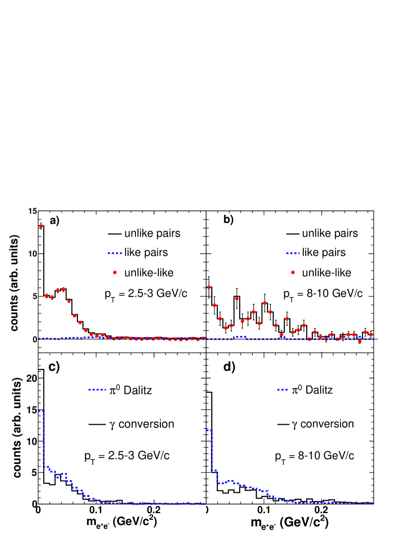
Refer to caption — Figure 1: (Color online) The upper two panels show the electron pair invariant mass distributions for electrons at 2.5 GeV/ $c<p_{T}<$ 3.0 GeV/ $c$ (a) and at 8.0 GeV/ $c<p_{T}<$ 10.0 GeV/ $c$ (b). Solid and dashed lines represent unlike-sign and like-sign pairs, respectively. Closed circles represent the difference of unlike and like. The lower two panels show the simulated invariant mass spectra with electrons at 2.5 GeV/ $c<p_{T}<$ 3.0 GeV/ $c$ (c) and at 8.0 GeV/ $c<p_{T}<$ 10.0 GeV/ $c$ (d). Solid and dashed lines represent results from $\gamma$ conversions and $\pi^{0}$ Dalitz decay.

Electron pairs are formed by combining an electron with $p_{T}>2.5$ GeV/ $c$ , which we refer to as a primary electron, with all other electrons (partners) reconstructed in the same event, with opposite charge sign (unlike-sign) or same charge sign (like-sign). The upper two panels of Fig. 1 show the invariant mass spectra for primary electrons with 2.5 GeV/ $c<p_{T}<$ 3.0 GeV/ $c$ (left) and 8.0 GeV/ $c<p_{T}<$ 10.0 GeV/ $c$ . The unlike-sign spectrum includes pairs originating from photon conversion and Dalitz decay, as well as combinatorial background. The latter can be estimated using the like-sign pair spectrum. The photonic electron spectrum is obtained by subtracting like-sign from unlike-sign spectrum (unlike-minus-like). The broad shoulders extending toward higher masses in the spectra are caused by finite tracking resolution, which leads to a larger reconstructed opening angle when the reconstructed track helices of two conversion electrons intersect each other in the transverse plane. The overall width of the mass spectra depends on the primary electron $p_{T}$ , but most photonic pairs are contained in range of $m_{ee}<0.24$ GeV/ $c^{2}$ . The lower two panels of Fig. 1 show the simulated invariant mass spectra of the two dominant sources of photonic electrons, $\pi^{0}$ Dalitz and $\gamma$ conversions, in the same two $p_{T}$ regions, which are similar in shape due to similar decay kinematics. The electron spectrum obtained from the unlike-minus-like method is from pure photonic electrons because the combinatorial background is accurately described by the like-sign pair spectrum according to the simulation and the simulated mass spectra are in qualitative agreement with the data. This is also proved by the fact that the distribution of the normalized ionization energy loss (see Sec. III.2) can be well described by a Gaussian function expected from electrons as shown in Fig. 4.

We calculate the yield of non-photonic electrons according to

N(npe)=N(inc)\cdotp\epsilon_{purity}-N(pho)/\epsilon_{pho},

where $N(npe)$ is the non-photonic electron yield, $N(inc)$ is the inclusive electron yield, $N(pho)$ is the photonic electron yield, $\epsilon_{pho}$ is the photonic electron reconstruction efficiency defined as the fraction of the photonic electrons identified through invariant mass reconstruction, and $\epsilon_{purity}$ is the purity reflecting hadron contamination in the inclusive electron sample.

Electrons from open heavy flavor decays dominate non-photonic electrons. The contribution from semi-leptonic decay of kaons is negligible for $p_{T}>$ 2.5 GeV/ $c$ Adare:2006hc . Electrons from vector mesons ( $\rho,\omega,\phi$ , $J/\psi$ , $\Upsilon$ ) decays and Drell-Yan processes are subtracted from the measurement (see Sec. III.7 for details).

III.2 Electron Reconstruction and Identification Efficiency

In the analysis of the Run2008 data, we select only tracks with $p_{T}>2.5$ GeV/ $c$ and $|\eta|<0.5$ . The event vertex position along the beam-axis ( $V_{z}$ ) is required to be close to the center of the TPC, i.e. $|V_{z}|<30$ cm. To avoid track reconstruction artifacts, such as track splitting, the selected tracks are required to have at least $52\%$ of the maximum number of TPC points allowed in the TPC, a minimum of 20 TPC points and a distance-of-closest-approach (DCA) to the collision vertex less than 1.5 cm. For hadron rejection we apply a cut of $n\sigma_{e}>-1$ on the normalized ionization energy loss in the TPC dedx , which is defined as

n\sigma_{e}=\log((dE/dx)/B_{e})/\sigma_{e},

where $B_{e}$ is the expected mean $dE/dx$ of an electron calculated from the Bichsel function bichsel and $\sigma_{e}$ is the TPC resolution of $\log((dE/dx)/B_{e})$ .

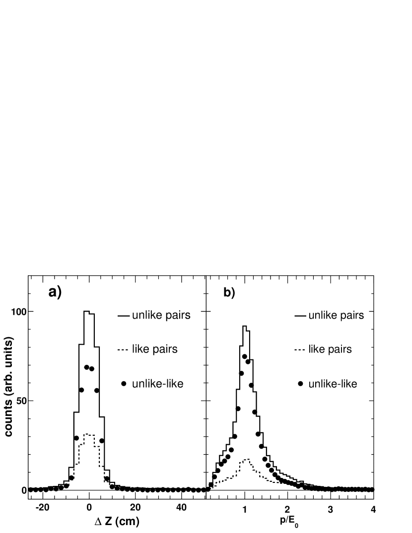
We reconstruct clusters in the BEMC and the BSMD by grouping adjacent hits that are likely to have originated from the same incident particle bemc_cvs_cluster . The selected tracks are extrapolated to the BEMC and the BSMD where they are associated with the closest clusters. The association windows for electrons are determined by measuring the distance between the track projection point at the BEMC (BSMD) and the closest BEMC (BSMD) cluster using photonic electrons from the unlike-minus-like pairs. Figure 2 (a) shows the distribution of this distance at the BEMC along the beam direction for electrons from unlike-sign, like-sign and unlike-minus-like pairs requiring $m_{e^{+}e^{-}}<0.24$ GeV/ $c^{2}$ , a maximum 1.0 cm DCA between two helical-shaped electron tracks and a 3.0 keV/cm $<dE/dx<$ 5.0 keV/cm cut on ionization energy loss for partner tracks. Most electrons are inside a window of $\pm 20$ cm around the track projection point. The window in the azimuthal plane is determined to be $\pm 0.2$ radian. Figure 2 (b) shows the distribution of $p/E_{0}$ for electrons from unlike-sign, like-sign and unlike-minus-like pairs, where $E_{0}$ is the energy of the most energetic tower in a BEMC cluster. The distribution is peaked around one due to the small mass of the electron and the fact that most electron energy is deposited into one tower. We apply a cut of $p/E_{0}<$ 2.0 to further reduce hadron contamination. Cuts on the association with BSMD clusters are kept loose to maintain high efficiency. Each track is required to have more than one associated BSMD strip in both $\phi$ and $\eta$ planes.

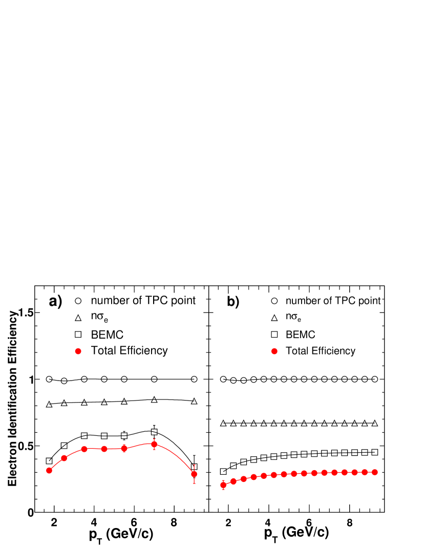
The efficiencies of electron identification cuts are estimated directly from the data using pure photonic electrons obtained from the unlike-minus-like pairs requiring $m_{e^{+}e^{-}}<0.24$ GeV/ $c^{2}$ , a maximum 1.0 cm DCA between two helical-shaped electron tracks and a 3.0 keV/cm $<dE/dx<$ 5.0 keV/cm cut on ionization energy loss for partner tracks. A cut of $p_{T}>0.3$ GeV/ $c$ for partners is also applied, selecting a region where the simulation does a good job of describing the data. The efficiency for one specific cut is then calculated as the ratio of electron yield before the cut to that after the cut, while all the other electron identification cuts are applied. To avoid possible correlation among different cuts, efficiencies for all BEMC and BSMD cuts are calculated together. Figure 3 (a) shows the breakdown of the electron identification efficiency as a function of $p_{T}$ . The drop in the low $p_{T}$ region comes mainly from BSMD inefficiency, while the drop in the high $p_{T}$ region is caused by the $p/E_{0}$ cut. The uncertainties in the figure are purely statistical and are included as part of the systematic uncertainties for the cross section calculation.

To maintain high track quality and suppress photonic electrons from conversion in the TPC gas, we require the radial location of the first TPC point to be less than 70 cm. This cut causes an inefficiency of $12.0\pm 2.0\%$ for non-photonic electrons according to the estimates from both simulation and data.

Through embedding simulated electrons into high-tower trigger events and processing them through the same software used for data production, single electron reconstruction efficiency in the TPC is found to be 0.84 $\pm$ 0.04 with little dependence on momentum for $p_{T}>$ 2.0 GeV/ $c$ .

The analysis of the Run2005 data is slightly different from that of the Run2008 described above. Only half of the BEMC (0 $<\eta<$ 1.0) was instrumented in 2005. Due to the presence of the silicon detectors, and their significant material budget, photonic backgrounds were substantially higher. We select only tracks with $0<\eta<0.5$ from -30 cm $<V_{z}<$ 20 cm in order to avoid the supporting cone for the silicon detectors in the fiducial volume while keeping track quality cuts identical to those in the Run2008 analysis. However, we apply a tighter cut on the normalized ionization energy loss, i.e. $-0.7<n\sigma_{e}<3.0$ , to improve hadron rejection. BEMC clusters are grouped with geometrically overlapping BSMD clusters to improve position resolution and electron hadron discrimination through shower profile. The clustering algorithm is also modified to increase the efficiency of differentiating two overlapping BSMD clusters by lowering the energy threshold of the second cluster bemc_ucla_cluster . The minimum angle between track projection point at the BEMC and all BEMC clusters is required to be less than $0.05$ radian. We also require each track to have more than one associated BSMD strip in both $\phi$ and $\eta$ planes, and a tightened $p/E$ cut of $0.3<p/E<1.5$ , where $E$ is the energy of the associated BEMC cluster. The efficiencies for the electron identification cuts are estimated by embedding simulated single electrons into minimum-bias PYTHIA pythia_doc events. Figure 3 (b) shows the breakdown of electron identification efficiency as a function of $p_{T}$ in the Run2005 analysis. There is no drop at high $p_{T}$ as in the Run2008 result because the energy of a whole BEMC cluster, instead of the highest tower, is used for the $p/E$ cut. No cut on the first TPC point is applied in this analysis. To avoid the TPC tracking resolution effect that causes the broad shoulder extending toward higher masses in the invariant mass spectrum of the Run2008 analysis, we utilize a 2-D invariant mass by ignoring the opening angle in the $\phi$ plane when reconstructing the $e^{+}e^{-}$ invariant mass bemc_ucla_cluster . We require $-3<n\sigma_{e}<3$ for partner tracks, 2-D $m_{e^{+}e^{-}}<0.1$ GeV/ $c^{2}$ for pairs, a maximum 0.1/0.05 radian for the opening angle in the $\phi$ / $\theta$ plane, and a maximum 1.0 cm DCA between two electron helices. A cut of $p_{T}>0.3$ GeV/ $c$ for partners is also applied so that the simulation can describe the data well.

By following independent analysis procedures from two RHIC runs where the amount of material for photonic background is significantly different, we will be able to validate our approach for measuring non-photonic electron production.

III.3 Purity Estimation

After applying all electron identification cuts, the inclusive sample of primary electrons is still contaminated with hadrons. To estimate the purity of electrons in the inclusive sample, we perform a constrained fit on the charged track $n\sigma_{e}$ distributions in different $p_{T}$ regions with three Gaussian functions representing the expected distributions of $\pi^{\pm}$ , $K^{\pm}+p^{\pm}$ and $e^{\pm}$ . The purity is estimated from the fit.

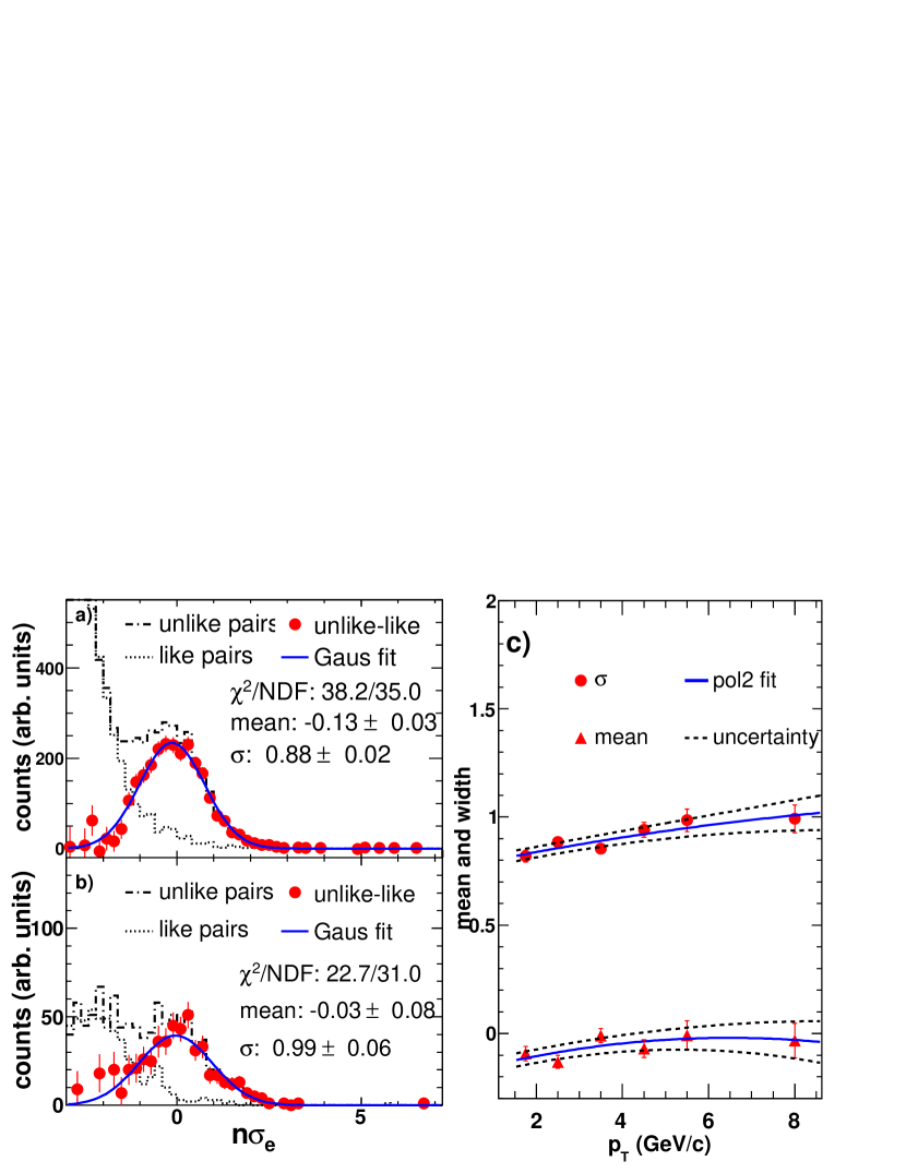
Ideally the electron $n\sigma_{e}$ will follow the standard normal distribution. The actual distribution can be slightly different due to various effects in data calibrations. We can, however, determine its shape in different $p_{T}$ regions directly from data using photonic electrons from the unlike-minus-like pairs. The left panel of Fig. 4 shows the $n\sigma_{e}$ distribution for tracks with (a) 2.5 GeV/ $c<p_{T}<3.0$ GeV/ $c$ and (b) 8.0 GeV/ $c<p_{T}<10.0$ GeV/ $c$ from unlike-sign, like-sign pairs as well as for photonic electrons from the unlike-minus-like pairs. Here all electron identification cuts, except the $n\sigma_{e}$ cut, are applied. The $n\sigma_{e}$ of photonic electrons are well fitted with Gaussian functions. Figure 4 (c) shows the mean and width of the Gaussian fit as a function of electron $p_{T}$ , which, as discussed above, differ slightly from the ideal values. The solid lines in the figure are fits to the data using a second order polynomial function. The dotted lines are also second order polynomial fits to the data except that the data points are moved up and down simultaneously by one standard deviation. The region between the dotted lines represents a conservative estimate of the fit uncertainty since we assume that the points are fully correlated. The mean, width and their corresponding uncertainties from the fits are used to define the shape of electron $n\sigma_{e}$ distribution in the following 3-Gaussian fit. The $n\sigma_{e}$ of $\pi^{\pm}$ and $K^{\pm}+p^{\pm}$ are also expected to follow Gaussian distributions dedx . Ideally their width is one and their means can be calculated through the Bichsel function bichsel . These ideal values are used as the initial values of the fit parameters in the following 3-Gaussian fit.

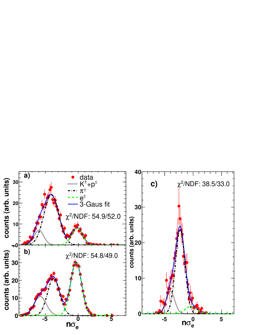
Figure 5 shows the constrained 3-Gaussian fits to the $n\sigma_{e}$ distributions of inclusive electron candidates with 2.5 GeV/ $c<p_{T}<3.0$ GeV/ $c$ in the Run2008 analysis (upper-left), 2.5 GeV/ $c<p_{T}<3.5$ GeV/ $c$ in the Run2005 analysis (lower-left) and 8.0 GeV/ $c<p_{T}<10.0$ GeV/ $c$ in the Run2008 analysis (right). Here we leave the $n\sigma_{e}$ cut open. The dotted, dot-dashed and dashed lines represent, respectively, the fits for $K^{\pm}+p^{\pm}$ , $\pi^{\pm}$ , and $e^{\pm}$ . Compared to the Run2008 analysis, the electron component in the Run2005 analysis at similar $p_{T}$ is more prominent due to the larger conversion electron yield. The solid lines are the overall fits to the spectra. The purity is calculated as the ratio of the integral of the electron fit function to that of the overall fit function above the $n\sigma_{e}$ cut. No constraints are applied to the $K^{\pm}+p^{\pm}$ and $\pi^{\pm}$ functions unless the fits fail. To estimate the systematic uncertainty of the purity, the mean and width of the electron function are allowed to vary up to one, two, three and four standard deviations from their central values. For each of the four constraints, we calculate one value of the purity. The final purity is taken as the mean and the systematic uncertainty is taken as the largest difference between the mean and the four values from the four constraints. To estimate the statistical uncertainty of the purity, we rely on a simple Monte-Carlo simulation. We first obtain a large sample of altered overall $n\sigma_{e}$ spectra by randomly shifting each data point in the original spectrum in Fig. 5 according to a Gaussian distribution with the mean and width set to be equal to the central value and the uncertainty of the original data point, respectively. We then obtain the purity distribution through calculating the purity from each of these altered spectra following the same procedure as discussed above. In the end, we fit the distribution with a Gaussian function and take its width as the statistical uncertainty. The total uncertainty of the purity is obtained as the quadratic sum of the statistical and systematic uncertainties.

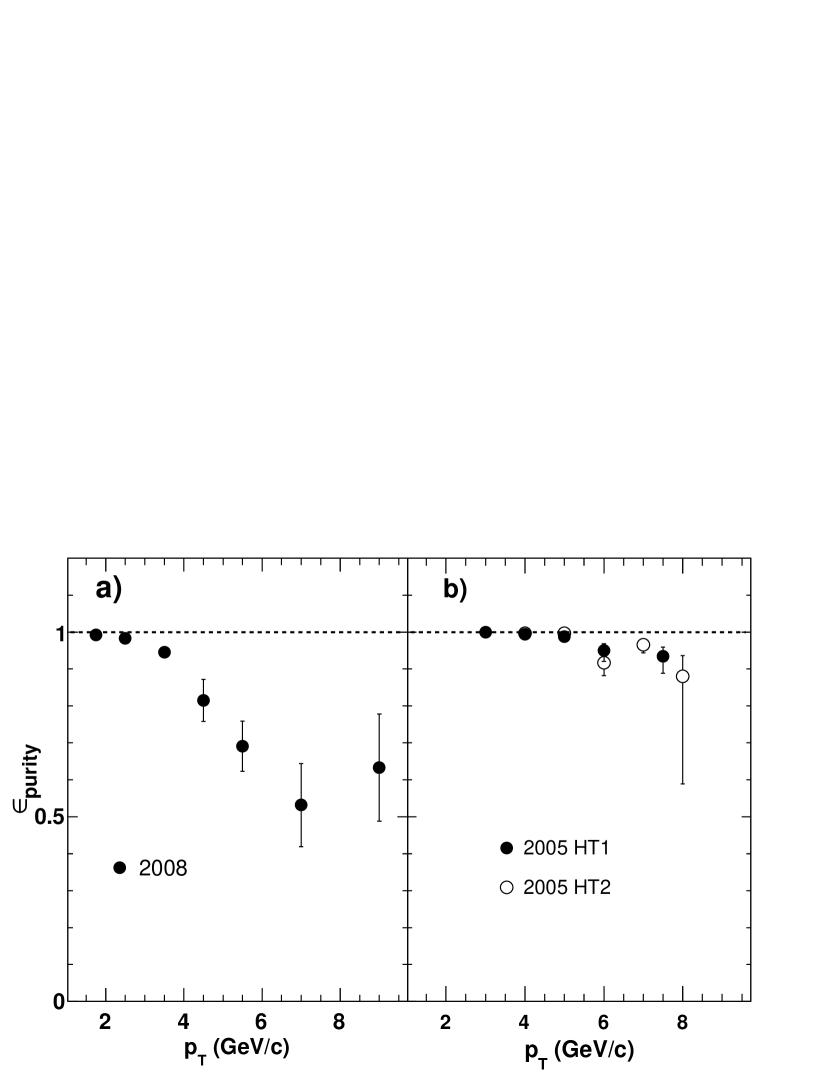
We follow the same procedure in the Run2008 and the Run2005 analysis except that the overall $n\sigma_{e}$ distribution in the Run2008 analysis is the combined result from the datasets of all three high-tower triggers as described Sec. II.3, while in the Run2005 analysis, the purity are calculated separately for the two high-tower triggers. Figure 6 shows the purity as a function of electron $p_{T}$ for the Run2008 (a) and the Run2005 (b) data. Tighter electron identification cuts and much higher photonic electron yield lead to much higher purity for the Run2005 inclusive electron sample.

III.4 Photonic Electron Reconstruction Efficiency

Since photon conversions, $\pi^{0}$ and $\eta$ meson Dalitz decays are the dominant sources of photonic electrons, they are the components that we used to calculate $\epsilon_{pho}$ , the photonic electron reconstruction efficiency, in the analysis of the Run2008 data. The $\epsilon_{pho}$ for each individual component is calculated separately to account for its possible dependence on the decay kinematics of the parent particles. The final $\epsilon_{pho}$ is obtained by combining results from all components according to their relative contribution to the photonic electron yield.

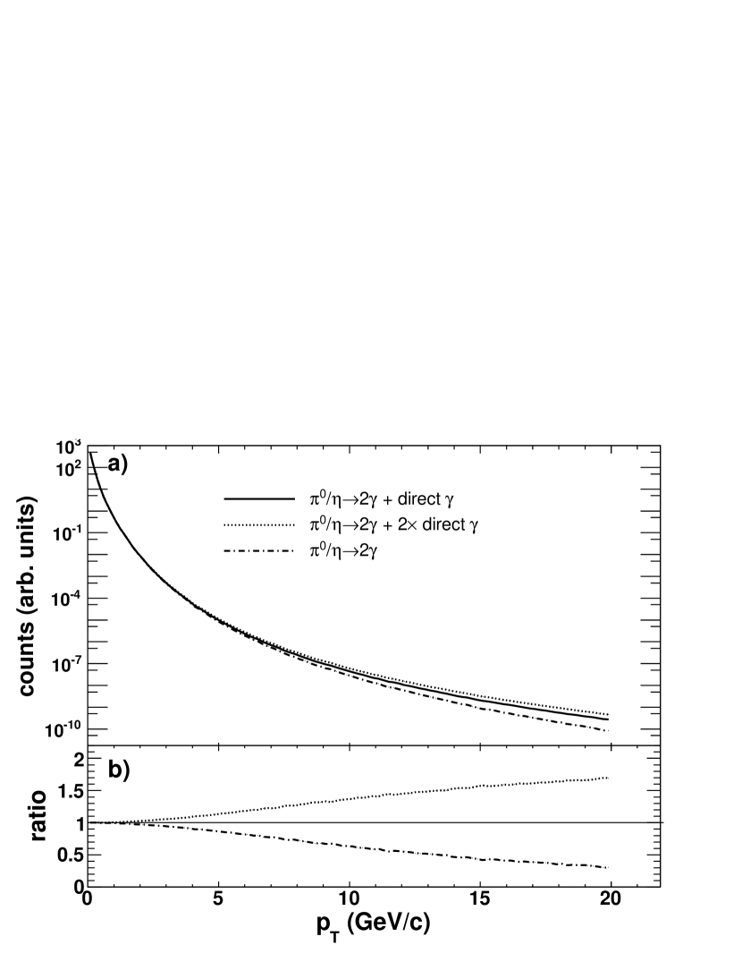
The determination of $\epsilon_{pho}$ is done through reconstructing electrons from simulated $\gamma$ conversion or Dalitz decay of $\pi^{0}$ and $\eta$ with uniform $p_{T}$ distributions that are embedded into high-tower trigger events. These events are then fully reconstructed using the same software chain as used for data analysis. To account for the efficiency dependence on the parent particle $p_{T}$ , we use a fit function to the measured $\pi^{0}$ spectrum, the derived $\eta$ and inclusive photon $p_{T}$ spectra as weights. The fit function to the measured $\pi^{0}$ spectrum is provided by the PHENIX experiment in Ref. phnx_dir_gamma . The $\eta$ spectrum is derived from the $\pi^{0}$ measurement assuming $m_{T}$ scaling, i.e. replacing $p_{T}$ with $\sqrt{p^{2}_{T}+m^{2}_{h}-m^{2}_{\pi^{0}}}$ while keeping the function form unchanged. Figure 7 (a) shows the derived inclusive $\gamma$ $p_{T}$ spectrum (solid line), and an estimate of its uncertainty represented by the region between the dotted and dot-dashed lines. Figure 7 (b) shows the uncertainty in linear scale. The inclusive $\gamma$ spectrum is obtained by adding the direct $\gamma$ yield to the $\pi^{0}$ and $\eta$ decay $\gamma$ yield calculated using PYTHIA. The direct $\gamma$ yield is obtained from the fit function to the direct $\gamma$ measurement provided by the PHENIX experiment in Ref. phnx_dir_gamma . The dot-dashed line represents the $\gamma$ spectrum from $\pi^{0}$ and $\eta$ decay alone. The dotted line is obtained by doubling the direct $\gamma$ component in the inclusive photon spectrum. By comparing the ratio of the derived inclusive $\gamma$ yield to that of $\pi^{0}$ and $\eta$ decay photon with the double ratio measurement in Au+Au most peripheral collisions phnx_dir_g_AuAu , we found the uncertainty covers the possible variations of the inclusive photon yield.

STAR simulations for $\gamma$ conversion and Dalitz decay are based on GEANT3 Brun:1987ma which incorrectly treats Dalitz decays as simple 3-body decays in phase space. We therefore modified the GEANT decay routines using the correct Kroll-Wada decay formalism Kroll:1955zu . Their kinematics is strongly modified by the dynamic electromagnetic structure arising at the vertex of the transition which is formally described by a form factor. We included the most recent form factors using a linear approximation for the $\pi^{0}$ Dalitz decay Amsler:2008zzb , and a pole approximation for the decays of $\eta$ :2009wb .

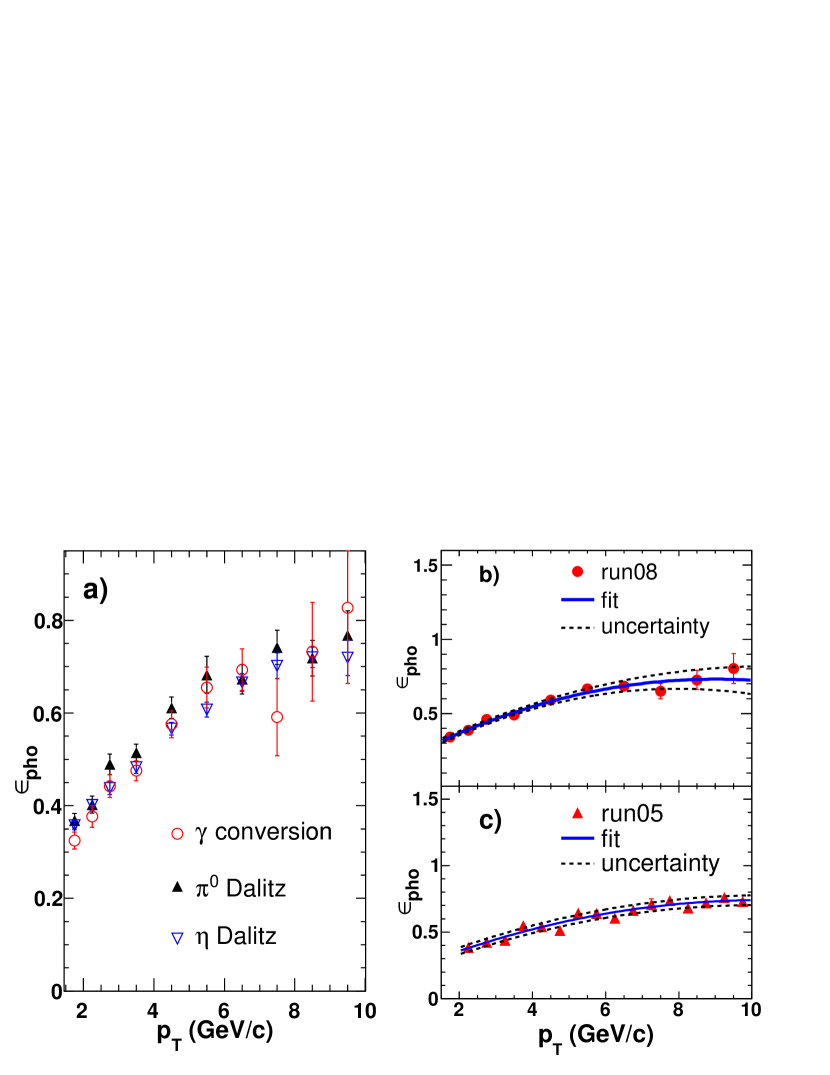
Figure 8 (a) shows the photonic electron reconstruction efficiency as a function of electron $p_{T}$ for $\gamma$ conversion, $\pi^{0}$ and $\eta$ Dalitz decay electrons, which turn out to be very similar because of the similar decay kinematics. The increase towards larger electron $p_{T}$ is due to the higher probability of reconstructing both electrons from high $p_{T}$ (virtual) photons. The uncertainties shown in the plots are dominated by the statistics of the simulated events. The effect due to the variation of the inclusive photon spectrum shape is found to be negligible for this analysis. Figure 8 (b) shows the combined photonic electron reconstruction efficiency for the Run2008 analysis, which is calculated as

	$\displaystyle\epsilon_{pho}(p_{T})=$		$\displaystyle\frac{N_{e}^{\gamma}(p_{T})}{N_{e}^{\gamma}(p_{T})+N_{e}^{\pi^{0}}(p_{T})+N_{e}^{\eta}(p_{T})}\cdotp\epsilon_{\gamma}(p_{T})+$
			$\displaystyle\frac{N_{e}^{\pi^{0}}(p_{T})}{N_{e}^{\gamma}(p_{T})+N_{e}^{\pi^{0}}(p_{T})+N_{e}^{\eta}(p_{T})}\cdotp\epsilon_{\pi^{0}}(p_{T})+$
			$\displaystyle\frac{N_{e}^{\eta}(p_{T})}{N_{e}^{\gamma}(p_{T})+N_{e}^{\pi^{0}}(p_{T})+N_{e}^{\eta}(p_{T})}\cdotp\epsilon_{\eta}(p_{T}),$

where $N_{e}^{\gamma}$ , $N_{e}^{\pi^{0}}$ and $N_{e}^{\eta}$ are respectively the yield of electrons from photon conversion, $\pi^{0}$ and $\eta$ Dalitz decay; $\epsilon_{\gamma}$ , $\epsilon_{\pi^{0}}$ and $\epsilon_{\eta}$ are the corresponding photonic electron reconstruction efficiencies. Based on Table 1, approximately $36\%$ of the photonic electrons are from $\pi^{0}$ Dalitz decay and about $10\%$ are from $\eta$ Dalitz decay. Their variations have negligible effect on the results since $\epsilon_{\gamma}$ , $\epsilon_{\pi^{0}}$ and $\epsilon_{\eta}$ are almost identical. The solid line is a second order polynomial fit to the data. The systematic uncertainty is represented by the region between the dotted lines, which are second order polynomial fits after moving all the data points simultaneously up and down by one standard deviation.

For the Run2005 analysis, the dominant source of photonic electrons is conversion in the silicon detectors. We therefore neglect contributions from Dalitz decays while following the same procedure as for the Run2008 analysis to calculate $\epsilon_{pho}$ . Figure 8 (c) shows $\epsilon_{pho}$ as a function of $p_{T}$ for $\gamma$ conversion for the Run2005 analysis. The solid line is a fit to the spectrum with a second order polynomial function and the region between dashed lines represents the uncertainty estimated in the same way as for the Run2008 analysis. The inclusion of the Dalitz decays is estimated to reduce the $\epsilon_{pho}$ by less than $0.5\%$ which is well within the systematic error. The uncertainty because of the inaccurate material distribution in the simulation as mentioned in Sec. II.2 is negligible since the majority of the material, dominated by our silicon detectors, is within a distance of 30 cm from beam pipe and the variation of $\epsilon_{pho}$ of photonic electrons produced within this region is small.

III.5 Trigger Efficiency

The trigger efficiency is the ratio of the electron yield from high-tower trigger events to that from minimum-bias trigger events after normalizing the two according to the integrated luminosity. To have a good understanding of trigger efficiency, one needs enough minimum-bias events for the baseline reference. However, for the Run2008 $p+p$ data, the number of minimum-bias events is too small to be used for this purpose. Fortunately the Run2008 d+Au data were taken using the same sets of high-tower triggers as used for $p+p$ run. Since the two data sets were taken serially, the high-tower trigger efficiency is expected to be the same. During the d+Au run, many events also were taken using the VPD trigger, which is essentially a less efficient minimum-bias trigger that can serve as the baseline reference for trigger efficiency analysis. As a cross check, we also evaluate the trigger efficiency through the Run2008 $p+p$ simulation.

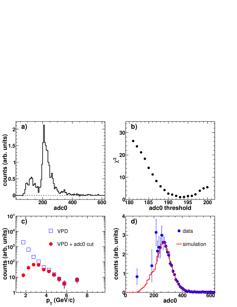
From the VPD trigger events, we first regenerate a high-tower trigger $p_{T}$ spectrum by requiring $adc0$ of BEMC clusters to be larger than the threshold. The $adc0$ is the offline ADC value of a BEMC cluster’s most energetic tower which is one of the high-towers responsible for firing a high-tower trigger. Figure 9 (a) shows the $adc0$ distribution of photonic electrons from high-tower trigger events. The sharp cut-off around a value of 200 is the offline ADC value of the trigger threshold setting. The smaller peak below the trigger threshold is due to electrons which happen to be in events triggered by something else other than the electrons. By requiring $adc0$ to be larger than the threshold, we reject these electrons which did not trigger the event since the uncertainty of their yield is affected by many sources and is therefore hard to be evaluated reliably. When the threshold is correctly chosen, the regenerated spectrum shape should be very similar to that of the actual high-tower trigger. We therefore quantitatively determine the trigger threshold as the $adc0$ cut which minimizes the

\chi^{2}=\displaystyle\sum_{i}(\frac{N_{i}(VPD+adc0)}{N_{i}(HT)}-1)^{2}/\sigma_{i}^{2}

where $N_{i}(VPD+adc0)$ is the regenerated high-tower trigger electron yield from VPD events in the $i^{th}$ $p_{T}$ bin, $N_{i}(HT)$ is the electron yield at the same $p_{T}$ bin from the actual high-tower trigger events, and $\sigma_{i}$ is the uncertainty of $N_{i}(VPD+adc0)$ . Figure 9 (b) shows the $\chi^{2}$ as a function of the $adc0$ cut; the threshold is taken as 193. Figure 9 (c) shows the $p_{T}$ spectrum of raw inclusive electrons from the VPD trigger (open squares) and the regenerated high-tower spectrum (closed circles) after applying the $adc0$ $>$ 193 cut used to calculate the trigger efficiency.

To estimate trigger efficiency through simulation, we tune the simulated single electron $adc0$ spectrum in each individual $p_{T}$ bin to agree with the data in the region above the threshold. The data spectra are obtained from the unlike-minus-like pairs, i.e. pure photonic electrons. As a demonstration of the comparison, Fig. 9 (d) shows the spectra from data (closed circles) and simulation (solid line) at 4.0 GeV/ $c<p_{T}<5.0$ GeV/ $c$ . The efficiency is defined as the fraction of the simulated $adc0$ spectrum integral above the trigger threshold.

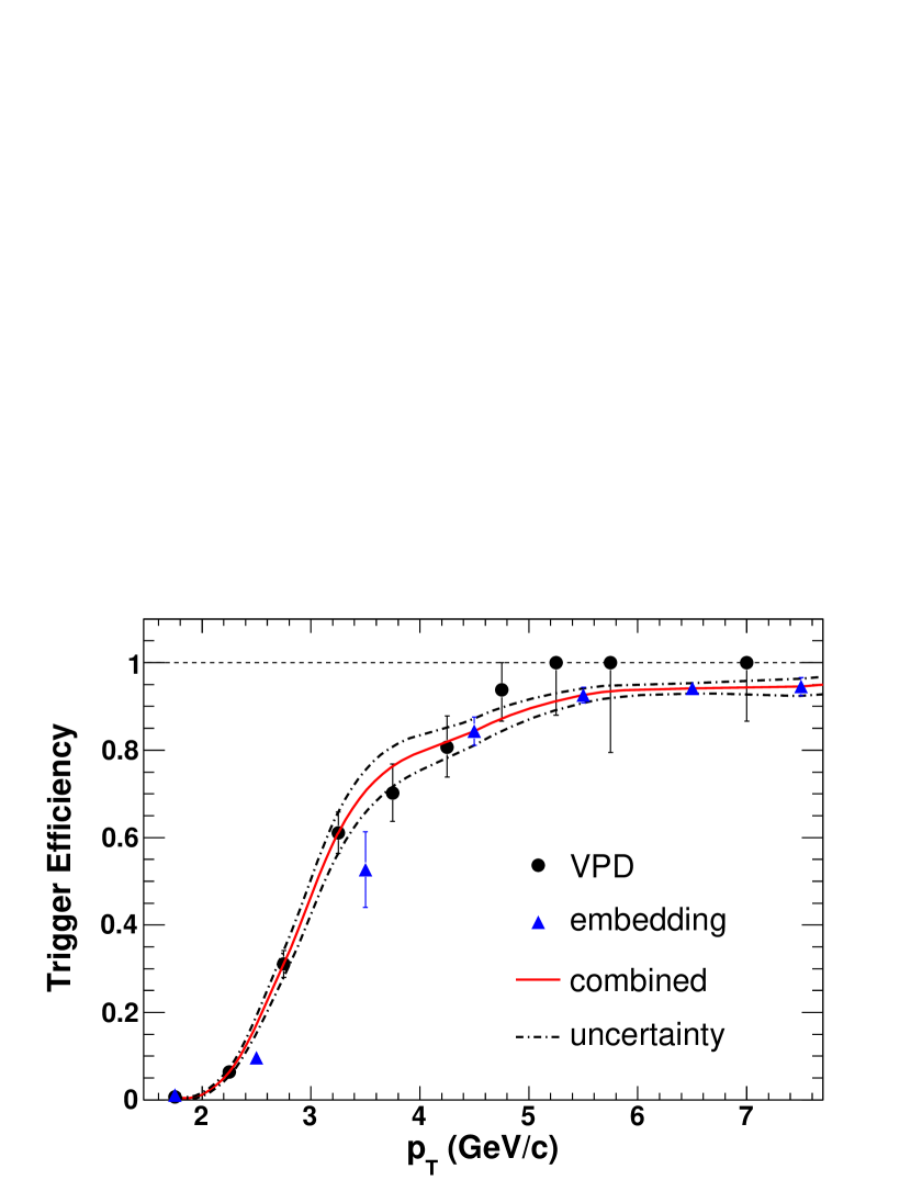
In the Run2008 analysis the raw $p_{T}$ spectrum of non-photonic electrons is obtained by combining the datasets of all three high-tower triggers. Since the shape of the combined spectrum is the same as that of the high-tower trigger with the lowest threshold, we only need to estimate the trigger efficiency of this lowest threshold trigger. Figure 10 shows the trigger efficiency as a function of $p_{T}$ that is calculated using d+Au VPD events (closed circles) and simulated events (closed triangles) in the Run2008 analysis. At $p_{T}>3.5$ GeV/ $c$ , they agree with each other reasonably well. At lower $p_{T}$ , the simulated results are not reliable because the numerator in the efficiency calculation is only from a tail of the spectrum and a small mismatch between simulation and data can have a large impact on the results. On the other hand, the results from VPD events suffer from low statistics at high $p_{T}$ . The final efficiency is therefore taken to be the combination of the two, i.e., at $p_{T}<3.5$ GeV/ $c$ , the efficiency is equal to that from VPD events assigning a systematic uncertainty identical to the statistical uncertainty of the data point, while at high $p_{T}$ , the efficiency is equal to the simulated results, and the systematic error are from the tuning uncertainty.

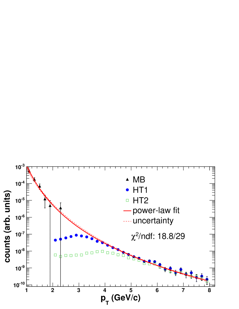
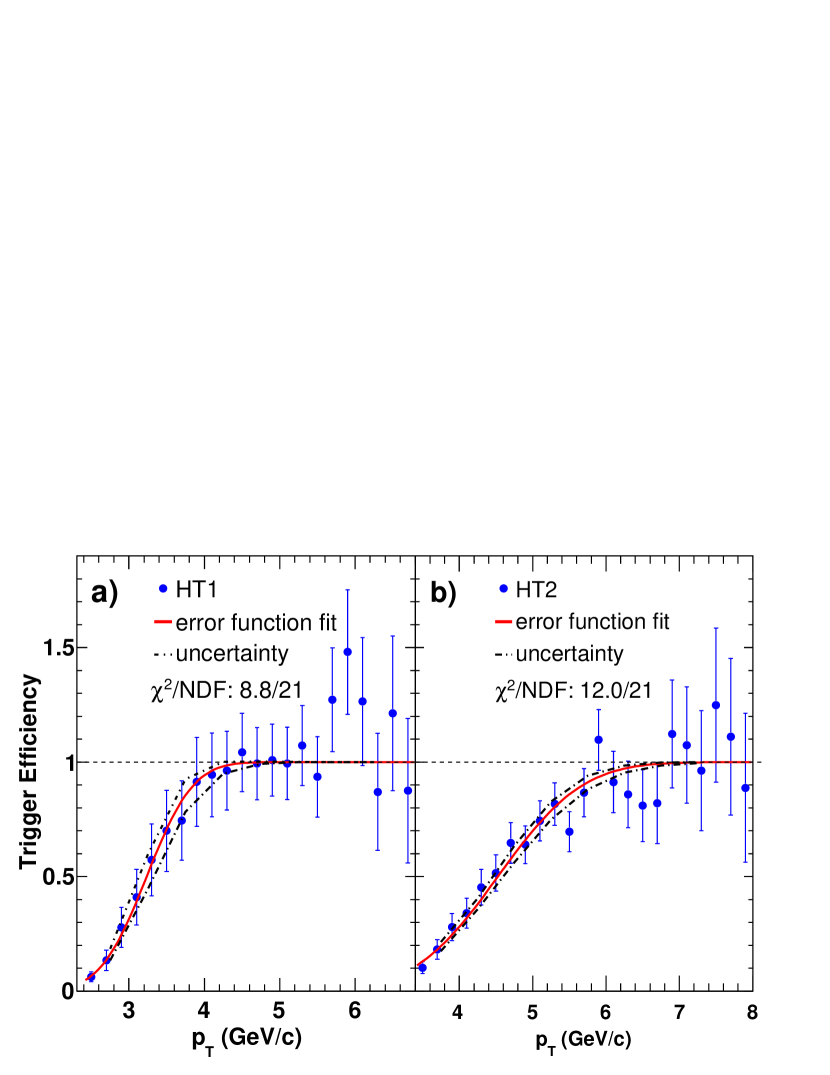
In the Run2005 analysis, the efficiencies of the two high-tower triggers are estimated separately. While there are more minimum-bias events for Run2005 than for Run2008, the statistics are poor at $p_{T}>2.0$ GeV/ $c$ . We thus rely on a fit to the spectrum, which consists of minimum-bias events at low $p_{T}$ and high-tower trigger events at high $p_{T}$ where the trigger is expected to be fully efficient, as the baseline reference for the trigger efficiency evaluation. Figure 11 shows the raw inclusive electron $p_{T}$ spectrum from minimum-bias, HT1 and HT2 events. The fit uses a power-law function $A(1+p_{T}/B)^{-n}$ . The regions where we expect HT1 and HT2 trigger to be fully efficient are above $4.5$ and $6.0$ GeV/ $c$ respectively. The dashed line shows the fit uncertainty, obtained from many fit trials. In a single fit trial, each data point is randomized with a Gaussian random number, with the mean to be the central value and the rms to be the statistical uncertainty of the data point. Additional systematic uncertainty coming from fits using different functions is included in the cross section calculation and is not displayed in the figure. Figure 12 shows the efficiency of HT1 (a) and HT2 (b) triggers, defined as the ratio of the raw HT1 or HT2 inclusive electron spectrum to the baseline fit function. We used error functions to parameterize both efficiencies. The dashed lines represent the uncertainty, obtained in the same way as for the Fig. 11 fits.

High-tower trigger efficiency for photonic and non-photonic electrons can be different. Unlike non-photonic electrons, a photonic electron always has a partner. In case both share the same BEMC tower, the deposited energy will be higher than that for an isolated electron and will lead to a higher efficiency. The effect can be quantified by comparing the ratio of the isolated electron yield to the yield of electrons with partners in minimum-bias events to the same ratio in high-tower trigger events. We found that the difference is negligible at $p_{T}>2.5$ GeV/ $c$ , while the trigger efficiency for photonic electron is $~{}20-30\%$ higher than for non-photonic electron in the lower $p_{T}$ region.

III.6 Stability of the Luminosity Monitor

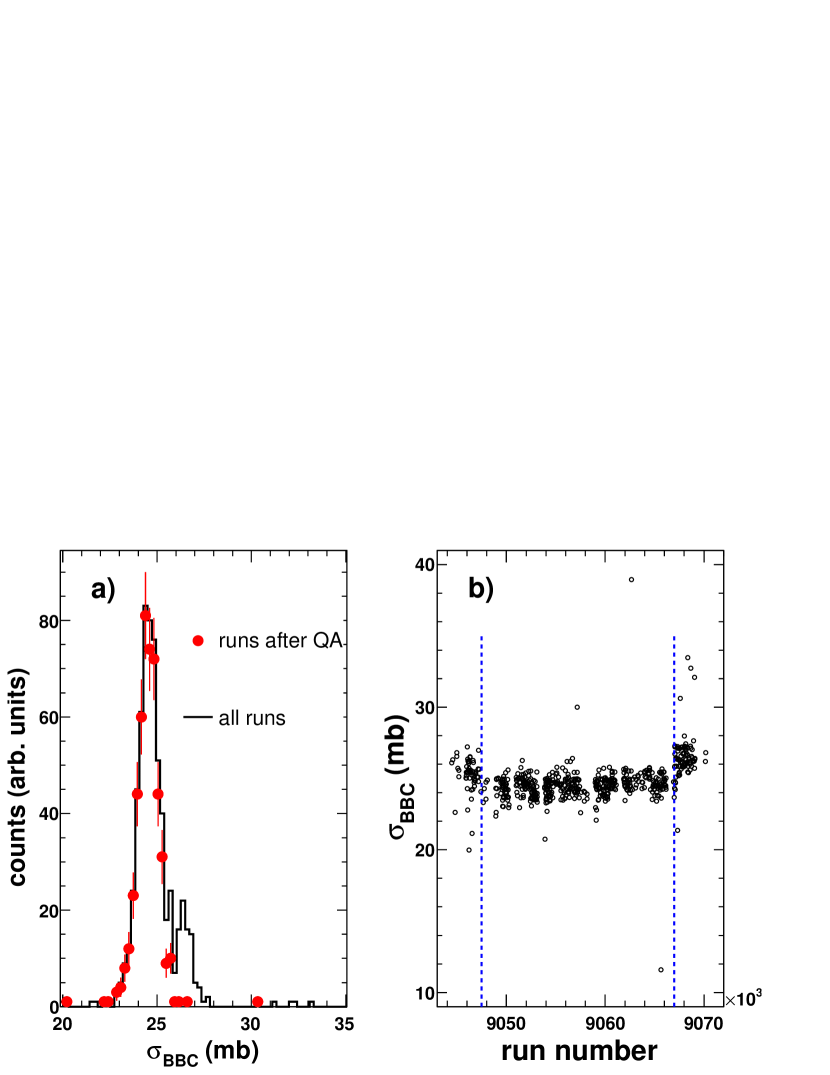
The BBC trigger was used to monitor the integrated luminosity for Run2005. During Run2008, because of the large beam background firing the BBC trigger, a high threshold high-tower trigger was used as the luminosity monitor. To quantify the stability of the monitor with respect to BBC, we calculate the BBC cross section as a function of run number using $\sigma_{BBC}=N_{minbias}/\cal L$ , where $\cal L$ $=N_{mon}/\sigma_{mon}$ , $\sigma_{mon}$ is the monitor cross section which is estimated to be $1.49$ $\mu$ b using low luminosity runs, $N_{minbias}$ and $N_{mon}$ are respectively the number of events from the BBC trigger and the monitor after correcting for prescaling during data acquisition. Here a run refers to a block of short term ( $\sim$ 30 minutes) data taking. Figure 13 (a) shows the distribution of the calculated $\sigma_{BBC}$ . There are two peaks in the figure. The dominant one centered around 25 mb contains most of the recorded luminosity in Run2008. The minor one centered at a higher value comes from events taken at the beginning and the end of Run2008 represented by the regions beyond the two dashed lines in Fig. 13 (b) showing the calculated BBC cross section as a function of run number. After removing these runs taken at the beginning and the end of Run2008, the minor peak disappeared and the performance of the monitor appeared to be very stable.

In the data analysis, we also reject those with $\sigma_{BBC}<20$ mb or $\sigma_{BBC}>30$ mb. We fit the $\sigma_{BBC}$ distribution with a Gaussian function and assign the width of the function ( $2.3\%$ ) as the systematic uncertainty of the $\sigma_{mon}$ with respect to BBC cross section.

The integrated luminosity sampled by the high-tower triggers are $\sim$ 2.6 pb^-1 and $\sim$ 2.8 pb^-1 for Run2008 and Run2005, respectively.

III.7 Contribution from Vector Mesons

The main background sources of electrons that do not originate from photon conversion and Dalitz decay are electromagnetic decays of heavy ( $J/\psi$ , $\Upsilon$ ) and light vector mesons ( $\rho$ , $\omega$ and $\phi$ ) as well as those from Drell-Yan process.

The electrons from $J/\psi$ decay contribute noticeably to the observed non-photonic electron signal as pointed out in Ref. Adare:2010de . In order to estimate the contribution from $\mbox{$J/\psi$}\rightarrow\mbox{$e^{+}e^{-}$}$ to the non-photonic electron yield, we combine the measured differential $J/\psi$ cross-sections from PHENIX Adare:2006kf and STAR Abelev:2009qaa . For each data point we add the statistical and systematic uncertainties, except the global uncertainties, in quadrature. Figure 14 (a) shows the measured $J/\psi$ differential cross section from the two experiments. While the PHENIX measurement dominates the low to medium- $p_{T}$ region, the STAR measurement dominates the high- $p_{T}$ region. The combined spectrum is fit using a power-law function of the form $Ed^{3}\sigma/d^{3}p|_{y=0}=A(\exp(a\mbox{$p_{T}$}-b\mbox{$p_{T}$}^{2})+p_{T}/p_{0})^{-n}$ where $A$ = 5.24 $\pm$ 0.87 mb $\cdot{\rm GeV^{-2}}c^{3}$ , $a$ = 0.32 $\pm$ 0.04 ${\rm GeV^{-1}}c$ , $b$ = 0.06 $\pm$ 0.03 ${\rm GeV^{-2}}c^{2}$ , $p_{0}$ = 2.59 $\pm$ 0.21 GeV/ $c$ and $n$ = 8.44 $\pm$ 0.61 are fit parameters. The $\chi^{2}$ /NDF of the fit is 27.8/25. To obtain the uncertainty of the fit, the global uncertainties of the STAR and the PHENIX (10% cesar ) measurements are assumed to be uncorrelated. We move the PHENIX data up by 10% and repeat the fit to obtain the band of 68% confidence intervals. The upper edge of the band is treated as the upper bound of the fit. Following the same procedure except moving the PHENIX data down by 10%, we obtain the lower bound of the fit as the lower edge of the band. Furthermore, since we are considering a rather large $p_{T}$ range ( $p_{T}<14.0$ ${\mathrm{GeV/}}c$ ), we cannot assume that the $p_{T}$ and rapidity distributions factorize. We use PYTHIA to generate $dN/dy(p_{T})$ and implement a Monte-Carlo program using the above functions as probability density functions to generate $J/\psi$ and decay them into $e^{+}e^{-}$ assuming the $J/\psi$ to be unpolarized. The decay electrons are filtered through the same detector acceptance as used for the non-photonic electrons. The band in Fig. 14 (b) shows the invariant cross section of $J/\psi$ decay electrons as a function of the electron $p_{T}$ . The uncertainty of the derived yield comes from the uncertainty of the fit to the $J/\psi$ spectra and is represented by the band which is also shown in Fig. 14 (c) in linear scale.

The invariant cross section of electrons from $\Upsilon$ decays ( $\Upsilon\rightarrow e^{+}e^{-}$ ), represented by the dot-dashed line in Fig. 14 (b), is calculated in a similar fashion as that for the $J/\psi$ except that the input $\Upsilon$ spectrum is from a Next-to-Leading Order pQCD calculation in the color evaporation model (CEM) vogt_upslion . We have to rely on model calculations since so far no invariant $p_{T}$ spectrum in our energy range has been measured. However, in a recent measurement STAR reported the overall production cross section for the sum of all three $\Upsilon$ (1S+2S+3S) states in $p$ + $p$ collisions at $\sqrt{s}$ = 200 GeV to be $B\times d\sigma/dy=114\pm 38^{+23}_{-24}$ pb, which is consistent with the CEM prediction Abelev:2010am . Adding the statistical and systematic uncertainty in quadrature, the total relative uncertainty of this measurement is $\sim$ 39%, which is the value we assigned as the total uncertainty of the $\Upsilon$ feed-down contribution to the non-photonic electrons at all $p_{T}$ .

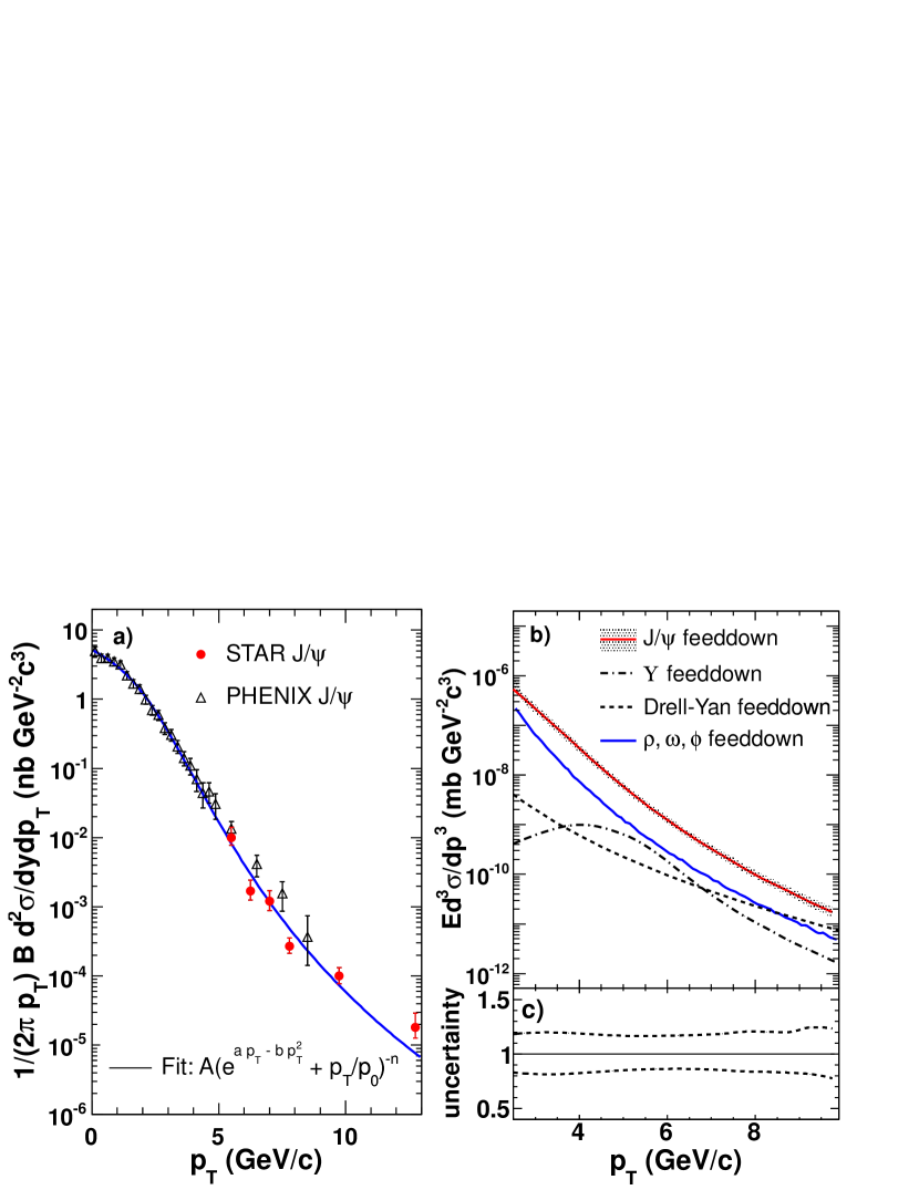
The contribution to the non-photonic electron yield from the light vector mesons is estimated using PYTHIA, assuming the meson spectra follow $m_{T}$ scaling. We generate a sample of decay electrons using light vector mesons with flat spectra in $p_{T}$ as input. To derive the differential cross section of the electrons, we keep only those electrons within the same detector acceptance as that for the non-photonic electrons and weight them with the spectra of $\rho$ , $\omega$ and $\phi$ . The meson spectra are obtained by replacing the $p_{T}$ with $\sqrt{p^{2}_{T}+m^{2}_{h}-m^{2}_{\pi^{0}}}$ in the same fit function as for the $\pi^{0}$ measurement (see Fig. 7). Here $m_{h}$ is the mass of the vector meson. The relative yields of the mesons to $\pi$ Adare:2006hc are also taken into account during this process. We include the decay channels $\phi\rightarrow e^{+}e^{-}$ , $\phi\rightarrow\eta e^{+}e^{-}$ , $\omega\rightarrow e^{+}e^{-}$ , $\omega\rightarrow\pi^{0}e^{+}e^{-}$ and $\rho\rightarrow e^{+}e^{-}$ in the calculation. The derived electron differential cross section is represented by the solid line in Fig. 14 (b). We assign a 50 $\%$ systematic uncertainty to cover the uncertainty of the $\pi^{0}$ measurement and the meson to pion ratios.

The contribution to the non-photonic electron yield from the Drell-Yan processes is represented by the dotted line in Fig. 14 (b) and is estimated from a Leading-Order pQCD calculation using the CTEQ6M parton distribution function with a K-factor of 1.5 applied and without a cut on the electron pair mass werner . No uncertainty is assigned to this estimate.

IV Results

IV.1 Non-photonic Electron Invariant Cross Section

The invariant cross section for non-photonic electron production is calculated according to

E\frac{d^{3}\sigma}{dp^{3}}\,=\,\frac{1}{\cal L}\,\frac{1}{{2\pi}\,{p_{T}}\,{\Delta}p_{T}\,{\Delta}y}\,\frac{N_{npe}}{{\epsilon_{rec}}\,{\epsilon_{trig}}\,{\epsilon_{eid}}\,{\epsilon_{BBC}}},

where $N_{npe}$ is the non-photonic electron raw yield with the $V_{z}$ cuts, $\epsilon_{rec}$ is the product of the single electron reconstruction efficiency and the correction factor for momentum resolution and finite spectrum bin width, $\epsilon_{trig}$ is the high-tower trigger efficiency, $\epsilon_{eid}$ is the electron identification efficiency, $\cal L$ is the integrated luminosity with the $V_{z}$ cuts and $\epsilon_{BBC}=0.866\pm 0.08$ is the BBC trigger efficiency. The systematic uncertainties of all these quantities are listed in Table 2. The relative uncertainty of $\cal L\cdot$ $\epsilon_{BBC}$ in maximum range is 14% including uncertainties in tracking efficiency bbc_cross_section . Assuming a flat distribution within the range, we estimate the $\cal L\cdot$ $\epsilon_{BBC}$ uncertainty to be 8.1% in one standard deviation. The uncertainty of $N_{npe}$ is the quadratic sum of the uncertainties from the estimation of $\epsilon_{pho}$ , purity and the light vector meson contribution. The uncertainty of $\epsilon_{rec}$ is the quadratic sum of the uncertainties from correcting the track momentum resolution, the finite spectrum bin width as well as the estimation of single electron reconstruction efficiency. The range of the uncertainty for each individual quantity covers the variation of the uncertainty as a function of $p_{T}$ . In order to compare with the result in Ref. Abelev:2006db ; Adare:2006hc , we do not subtract the $J/\psi$ , $\Upsilon$ and Drell-Yan contribution from the non-photonic electron invariant cross section shown in Fig. 15 and Fig. 16.

Table 2: Sources of systematic uncertainty for the non-photonic electron invariant yield in

p+p

collisions. Type A are point to point uncertainties. Type B are scaling uncertainties which move data points in the same direction. Type C are the scaling uncertainties that are common to both Run2008 and Run2005. The range in each individual source covers the variation of the systematic uncertainty as a function of

p_{T}

source	Run2008	Run2005
$N_{npe}$	5.0-48.1 % (A)	8.5-38.0 % (A)
$\epsilon_{eid}$	6.5-25.2 % (A)	0.7-2.0 % (A)
$\epsilon_{trg}$	1.8-10.0 % (A)	0.3-16 % (A)
	5.4 % (B)
$\epsilon_{rec}$	2.3-33.3 % (A)	1.0-3.5 % (A)
	15.7 % (B)	11.0 % (B)
$\cal L\cdot$ $\epsilon_{BBC}$	2.3 % (B)
	8.1 % (C)	8.1 % (C)

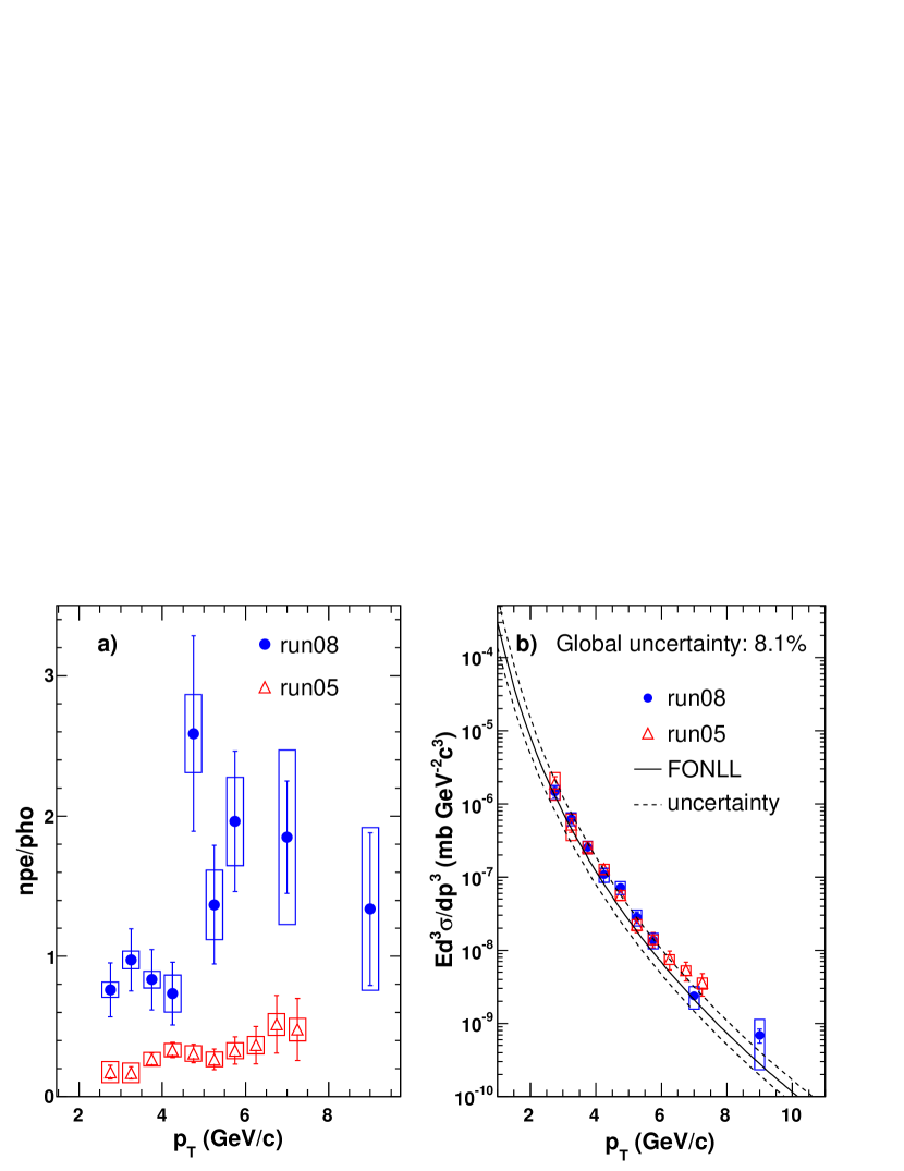
Figure 15 (a) shows the ratio of non-photonic to photonic electron yield as a function of $p_{T}$ in $p+p$ collisions in Run2008 (closed circles) and Run2005 (open triangles). The ratio for Run2008 is much larger because there was much less material in front of the TPC for Run2008. Figure 15 (b) shows the non-photonic electron invariant cross section ( $\frac{e^{+}+e^{-}}{2}$ ) as a function of $p_{T}$ in $p+p$ collisions from the Run2008 analysis (closed circles) and the Run2005 analysis (open triangles). Despite the large difference in photonic background, the two measurements are in good agreement.

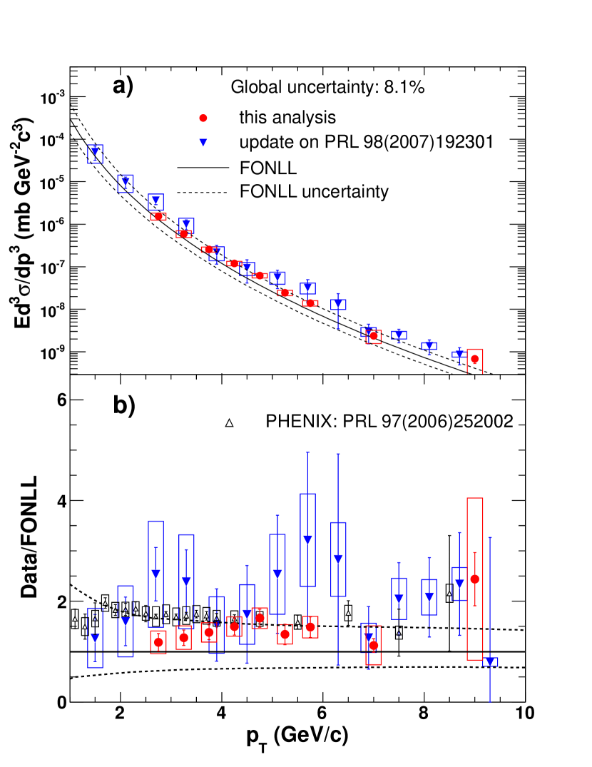
Figure 16 (a) shows the non-photonic electron ( $\frac{e^{+}+e^{-}}{2}$ ) invariant cross section obtained by combining the Run2008 and the Run2005 results using the “Best Linear Unbiased Estimate blue . The corrected result of our early published measurement using year 2003 data Abelev:2006db is shown in the plot as well. The published result exceeded pQCD predictions from FONLL calculations by about a factor of four. We, however, uncovered a mistake in the corresponding analysis in calculating $\epsilon_{pho}$ . The details are described in the erratum Abelev:2006db . To see more clearly the comparison, Fig. 16 (b) shows the ratio of each individual measurement, including PHENIX results, to the FONLL calculation. One can see that all measurements at RHIC on non-photonic electron production in $p+p$ collisions are now consistent with each other. The corrected run 2003 data points have large uncertainties because of the small integrated luminosity ( $\sim$ 100 nb^-1) in that run. FONLL is able to describe the RHIC measurements within its theoretical uncertainties.

IV.2 Invariant Cross Section of Electrons from
Bottom and Charm Meson Decays

Electrons from bottom and charm meson decays are the two dominant components of the non-photonic electrons. Mostly due to the decay kinematics, the azimuthal correlations between the daughter electron and daughter hadron are different for bottom meson decays and charm meson decays. A study of these azimuthal correlations has been carried out on STAR data and is compared with a PYTHIA simulation to obtain the ratio of the bottom electron yield to the heavy flavor decay electron yield ( $e_{B}/(e_{B}+e_{D})$ ) e_h , where PYTHIA was tuned to reproduce STAR measurements of D mesons $p_{T}$ spectra pythia_tune . Using the measured $e_{B}/(e_{B}+e_{D})$ , together with the measured non-photonic electron cross section with the electrons from $J/\psi$ , $\Upsilon$ decay and Drell-Yan processes subtracted, we are able to disentangle these two components.

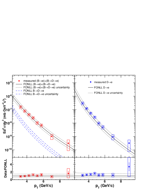
The bottom electron cross section is calculated as $e_{B}/(e_{B}+e_{D})$ times the non-photonic electron cross section with the contribution from $J/\psi$ , $\Upsilon$ decay and Drell-Yan processes subtracted. The same procedure applies to the charm electrons except that ( $1-e_{B}/(e_{B}+e_{D}))$ is used instead. The specific location of $p_{T}$ where the $e_{B}/(e_{B}+e_{D})$ is measured, is different from that of the non-photonic electrons. To accommodate the difference, we calculate $e_{B}/(e_{B}+e_{D})$ in any given $p_{T}$ in non-photonic electron measurements through a linear interpolation of the actual $e_{B}/(e_{B}+e_{D})$ measurements. As an estimation of the systematic uncertainty of the interpolated value, we also repeat the same procedure using the curve predicted by FONLL. Figure 17 shows the invariant cross section of electrons ( $\frac{e^{+}+e^{-}}{2}$ ) from bottom (upper-left) and charm (upper-right) mesons as a function of $p_{T}$ and the corresponding FONLL predictions, along with the ratio of each measurement to the FONLL calculations (lower panels). The statistical uncertainty of each data point is obtained by adding the relative statistical uncertainties of the corresponding data points in the non-photonic electron and the $e_{B}/(e_{B}+e_{D})$ measurement in quadrature. The systematic uncertainties are treated similarly, except that the uncertainties from the interpolation process are also included. The measured bottom electrons are consistent with the central value of FONLL calculation and the charm electrons are in between the central value and upper limit of the FONLL calculation, the uncertainties of which are from the variation of heavy quark masses and scales. From the measured spectrum, we determine the integrated cross section of electrons ( $\frac{e^{+}+e^{-}}{2}$ ) at 3 GeV/ $c<\mbox{$p_{T}$}<$ 10 GeV/ $c$ from bottom and charm meson decays to be, respectively,

{d\sigma_{(B\to e)+(B\to D\to e)}\over dy_{e}}|_{y_{e}=0}=4.0\pm 0.5({\rm stat.})\pm 1.1({\rm syst.}){\rm nb}

{d\sigma_{D\to e}\over dy_{e}}|_{y_{e}=0}=6.2\pm 0.7({\rm stat.})\pm 1.5({\rm syst.}){\rm nb},

where $y_{e}$ is the electron rapidity. The 8.1% global scale uncertainty from the BBC cross section is included in the total systematic uncertainty.

Relying on theoretical model predictions to extrapolate the measured results to the phase space beyond the reach of the experiment, one can estimate the total cross section for charm or bottom quark production. We perform a PYTHIA calculation with the same parameters as in Ref. Adams:2004fc . After normalizing the $p_{T}$ spectrum to our high- $p_{T}$ measurements and extrapolating the results to the full kinematic phase space, we obtain a total bottom production cross section of 1.34 $\mu$ b. However, with the PYTHIA calculation using the same parameters except MSEL=5, i.e. bottom production processes instead of minimum-bias processes as in the former calculation, we obtain a value of 1.83 $\mu$ b. The PYTHIA authors recommend the minimum-bias processes pythia_doc . This large variation between the extracted total bottom production cross sections comes mostly from the large difference in the shape of the bottom electron spectrum in the two PYTHIA calculations with MSEL=1 and with MSEL=5. Since both calculations are normalized to the measured data, the difference in the shape shows up at $p_{T}$ $<$ 3 GeV/ $c$ . The fact that the PYTHIA calculation with MSEL=5 only includes leading order diagrams of bottom production causes the difference between the PYTHIA calculations. Measurements in the low $p_{T}$ region are therefore important for the understanding of bottom quark production at RHIC. Both values are consistent with the FONLL Cacciari:2005rk prediction, $1.87^{+0.99}_{-0.67}\mu$ b, within its uncertainty.

V Conclusions

STAR measurements of high $p_{T}$ non-photonic electron production in $p+p$ collisions at $\sqrt{s}$ = 200 GeV using data from Run2005 and Run2008 agree with each other despite the large difference in background. This measurement and PHENIX measurement are consistent with each other within the quoted uncertainties. After correcting a mistake in the photonic electron reconstruction efficiency, the published STAR result using year 2003 data is consistent with our present measurements. We are able to disentangle the electrons from bottom and charm meson decays in the non-photonic electron spectrum using the measured ratio of $e_{B}/(e_{B}+e_{D})$ and the measured non-photonic cross section. The integrated bottom and charm electron cross sections ( $\frac{e^{+}+e^{-}}{2}$ ) at 3 GeV/ $c<\mbox{$p_{T}$}<$ 10 GeV/ $c$ are determined separately as

{d\sigma_{(B\to e)+(B\to D\to e)}\over dy_{e}}|_{y_{e}=0}=4.0\pm 0.5({\rm stat.})\pm 1.1({\rm syst.}){\rm nb}

{d\sigma_{D\to e}\over dy_{e}}|_{y_{e}=0}=6.2\pm 0.7({\rm stat.})\pm 1.5({\rm syst.}){\rm nb}.

FONLL can describe these measurements within its theoretical uncertainties. Future measurements on low- $p_{T}$ electrons from bottom meson decay are important to overcome the large uncertainties of the derived total bottom quark production cross section that originate mostly from the large variations of theoretical model prediction in the low- $p_{T}$ region.

Acknowledgements.

We thank the RHIC Operations Group and RCF at BNL, the NERSC Center at LBNL and the Open Science Grid consortium for providing resources and support. This work was supported in part by the Offices of NP and HEP within the U.S. DOE Office of Science, the U.S. NSF, the Sloan Foundation, the DFG cluster of excellence ‘Origin and Structure of the Universe’of Germany, CNRS/IN2P3, FAPESP CNPq of Brazil, Ministry of Ed. and Sci. of the Russian Federation, NNSFC, CAS, MoST, and MoE of China, GA and MSMT of the Czech Republic, FOM and NWO of the Netherlands, DAE, DST, and CSIR of India, Polish Ministry of Sci. and Higher Ed., Korea Research Foundation, Ministry of Sci., Ed. and Sports of the Rep. Of Croatia, and RosAtom of Russia.

References

(1) M. Cacciari, Nucl. Phys. A 783, 189 (2007).
(2) M. Cacciari, P. Nason and R. Vogt, Phys. Rev. Lett. 95, 122001 (2005); R. Vogt, private communication.
(3) S. Frixione, Eur. Phys. J. C 43, 103 (2005).
(4) A. D. Frawley, T. Ullrich and R. Vogt, Phys. Rept. 462, 125 (2008).
(5) M. G. Mustafa, D. Pal, D. K. Srivastava and M. Thoma, Phys. Lett. B 428, 234 (1998).
(6) M. Djordjevic, M. Gyulassy, R. Vogt and S. Wicks, Phys. Lett. B 632, 81 (2006).
(7) S. Wicks, W. Horowitz, M. Djordjevic and M. Gyulassy, Nucl. Phys. A 784, 426 (2007).
(8) M. Djordjevic and U. W. Heinz, Phys. Rev. Lett. 101, 022302 (2008).
(9) R. Sharma, I. Vitev and B. W. Zhang, Phys. Rev. C 80, 054902 (2009).
(10) G. D. Moore and D. Teaney, Phys. Rev. C 71, 064904 (2005).
(11) H. van Hees, V. Greco and R. Rapp, Phys. Rev. C 73, 034913 (2006).
(12) L. Grandchamp and R. Rapp, Nucl. Phys. A 715, 545 (2003).
(13) B. I. Abelev et al. [STAR Collaboration], Phys. Rev. D 79, 112006 (2009).
(14) S. Baumgart, Eur. Phys. J. C 62, 3 (2009).
(15) J. Adams et al. [STAR Collaboration], Phys. Rev. Lett. 94, 062301 (2005).
(16) B. I. Abelev et al. [STAR Collaboration], Phys. Rev. Lett. 98, 192301 (2007); B. I. Abelev et al. [STAR Collaboration], arXiv:nucl-ex/0607012v3 (2011).
(17) A. Adare et al. [PHENIX Collaboration], Phys. Rev. Lett. 97, 252002 (2006).
(18) S. S. Adler et al. [PHENIX Collaboration], Phys. Rev. Lett. 96, 032301 (2006).
(19) M. M. Aggarwal et al. [STAR Collaboration], Phys. Rev. Lett. 105, 202301 (2010).
(20) K. H. Ackermann et al., Nucl. Instr. Meth. A499, 624 (2003).
(21) M. Anderson et al., Nucl. Instr. Meth. A499, 659 (2003); M. Andersen et al., Nucl. Instr. Meth. A499, 679 (2003).
(22) M. Beddo et al., Nucl. Instr. Meth. A499, 725 (2003).
(23) J. Kiryluk [STAR Collaboration], 16th International Spin Physics Symposium Proc., 718 (2005).
(24) J. Adams et al. [STAR Collaboration], Phys. Rev. Lett. 91, 172302 (2003).
(25) W.J. Llope et al., Nucl. Instr. Meth. A522, 252 (2004).
(26) F. Jin [STAR Collaboration], J. Phys G36, 064051 (2009).
(27) B. I. Abelev et al. [STAR Collaboration], Phys. Rev. C81, 064904 (2010).
(28) Y. Xu, Olga Barannikova et al., arXiv:0807.4303v2 (2009).
(29) H. Bichsel, Nucl. Instr. Meth. A562, 154 (2006).
(30) W. Dong, Ph.D. thesis, (University of California Los
Angeles, 2006), http://drupal.star.bnl.gov/STAR/files/
startheses/2006/dong_weijiang.pdf.
(31) T. Sjostrand et al. JHEP 05, 026 (2006).
(32) A. Adare et al. [PHENIX Collaboration], Phys. Rev. C81, 034911 (2010); Y. Akiba, private communication.
(33) S. S. Adler et al. [PHENIX Collaboration], Phys. Rev. Lett. 94, 232301 (2005).
(34) GEANT 3.21, http://wwwasdoc.web.cern.ch/wwwasdoc/
geant_html3/geantall.html.
(35) N. M. Kroll and W. Wada, Phys. Rev. 98, 1355 (1955).
(36) C. Amsler et al. [Particle Data Group], Phys. Lett. B 667, 1 (2008).
(37) R. Arnaldi et al. [NA60 Collaboration], Phys. Lett. B 677, 260 (2009).
(38) A. Adare et al. [PHENIX Collaboration], arXiv:1005.1627 (2010).
(39) A. Adare et al. [PHENIX Collaboration], Phys. Rev. D 82, 012001 (2010).
(40) B. I. Abelev et al. [STAR Collaboration], Phys. Rev. C 80, 041902 (2009).
(41) C. L. D. Silva, private communication.
(42) R. Vogt, private communication.
(43) B. I. Abelev et al. [STAR Collaboration], Phys. Rev. D 82, 012004 (2010).
(44) W. Vogelsang, private communication.
(45) A. Valassi, Nucl. Instr. Meth. A500, 391 (2003).
(46) X. Lin, arXiv:hep-ph/0602067.

High pTsubscript𝑝𝑇p_{T} non-photonic electron production in p𝑝p+p𝑝p collisions at s𝑠\sqrt{s} = 200 GeV