Kagome Approximation for ${}^{3}He$ on Husimi Lattice with Two- and Three-Site Exchange Interactions

Abstract

The Ising approximation of the Heisenberg model in a strong magnetic field, with two-, and three-spin exchange interactions are studied on a Husimi lattice. This model can be considered as an approximation of the third layer of ${}^{3}He$ absorbed on the surface of graphite (kagome lattice). Using dynamic approach we have found exact recursion relation for the partition function. For different values of exchange parameters and temperature the diagrams of magnetization are plotted and showed that magnetization properties of the model vary from ferromagnetic to antiferromagnetic depending from the value of model parameters. For antiferromagnetic case magnetization plateau at $1/3$ of saturation field is obtained. Lyapunov exponent for recursion relation are considered and showed absents of bifurcation points in thermodynamic limit. The Yang-Lee zeros are analyzed in terms of neutral fixed points and showed that Yang-Lee zeros of the model are located on the arcs of the circle with the radius $R=1$.

1 Introduction

Since the spin-1/2 ${}^{3}He$ atoms have week attractive potential and light mass the zero-point fluctuations are large. Therefore helium can solidify only at very high pressures. Unlike usual solids, where the dominant is dipolar magnetic nuclear interaction in solid ${}^{3}He$ nucleon-nucleon interaction is dominant, therefore nuclear spins become ordered at 1 mK (for usual solids 1 microKelvin)[1]. For such systems theory of magnetism is based on multiple-spin exchange mechanism.

It is important to examine solid and fluid ${}^{3}He$ films absorbed on the surface of graphite,[3, 4, 5, 6] since it is a typical example of a two-dimensional frustrated quantum-spin system[7, 8]. The first and second layers of that system form triangular lattice, while the third one forms a system of quantum 1/2 spins on kagome lattice[9, 10, 11]. Both experimental[12, 13, 14] and theoretical[15, 16] studies indicate that three site exchange interaction is dominant in these systems. When the density of ${}^{3}He$ nuclei decreases the magnetic properties of system changes from ferromagnetic to antiferromagnetic one. This behavior can be explained in terms of multiple-spin exchange (MSE). For high densities the system is fully packed and three-site exchange interaction is dominant, therefore the system is ferromagnetic. When density decreases two-site exchange interaction becomes dominant and magnetic properties of the system change into antiferromagnetic one.

The magnetic properties were studied in Bose-Einstein condensates of ultracold atoms. The dynamical creation of fractionalized halt-quantum vortices in Bose-Einstein condensate of sodium atoms have been demonstrated[17]. Moreover, there were made the description of the Josephson effect in Abelian and non-Abelian Bose-Einstien condensate of alkali elements[18, 19]. Last of them may be realised in superfluid ${}^{3}He$ Josephson weak link[20]. The Kosterlitz-Thouless transition with random magnetic field[21] was used to describe marginal metal to insulator transition in disordered graphene[22].

At low temperatures antiferromagnetic quantum atoms of ${}^{3}He$ can exhibit plateaus on the magnetization curve. Beginning at some value of the external magnetic field (less than saturation field) the magnetization of the system does not change when the external magnetic field increase and system adsorbs energy without any change of magnetization. When the external magnetic field reaches a certain value the magnetization changes its value again.

This phenomena was theoretically predicted by Hida[23] for a ferromagnetic-ferromagnetic-antiferromagnetic Heisenberg chain 3CuCl${}_{2}\cdot$2 dioxane compound, which consists of the antiferromagnetic coupled trimers. For the different models the magnetization plateaus are predicted to occur in chains, ladders, within the dynamical and transfer matrix approaches (see Ref. [24]-[36]). For two dimensional systems appearance of magnetization plateaus has been found experimentally. On the triangular lattice a magnetization plateau was observed at $m/m_{s}=1/3$ for compounds like C₆Eu[37, 38], CsCuCl₃[39](see also Ref. [40]-[46]). For kagome lattice also have been observed magnetization plateau at 1/3 of saturation field[47, 48]. Noticeable, that plateaus appear only for the values of magnetization which are quantized to fraction values of the saturation magnetization. This phenomena was theoretically explained by Oshikawa, Yamanaka and Affleck[49] in 1997.

As mentioned above the third layer of the ${}^{3}He$ films absorbed on the surface of graphite is kagome lattice. Usually, the antiferromagnetic kagome lattice is investigated using numerical simulation[50, 51, 52]. In this paper dynamic system approach based on exact recursive relation for the partition function have been used. The key point of the approach is the so-called recursive lattice approximation[53], which is a very powerful tool in investigating many theoretical problems in statistical mechanics. We approximate kagome lattice by Husimi lattice which is a Bethe-type recursive lattice. This approach allows us to plot magnetization curves for different values of temperature and exchange parameters. For the finite size lattice at low temperature there are bifurcation points near plateaus, therefore Lyapunov exponent[54, 55, 56, 57] of recursion relation are studied to verify disappearance of the bifurcation points in thermodynamic limit.

In the strong external magnetic field Heisenberg model can be approximated by Ising one. There are not reasonable conditions in solid and fluid ${}^{3}He$ under which we could neglect the non-diagonal Heisenberg interaction, nevertheless, if the strong magnetic field is directed along the z-axis, we expect that it reduces the transverse fluctuations. It is supposed that in this case $\sigma^{x}$ and $\sigma^{y}$-spin components are infinitely small and these spin components can be neglected[1, 25, 27].

The knowledge of the partition function is very important in statistical mechanics, since the thermodynamic functions of the system can be expressed by means of the partition function. When the system undergoes phase transition, some thermodynamic functions (such as free energy) become nonanalytic at that point, therefore phase transitions can be associated with zeroes of partition function. In 1952 for the first time Yang and Lee[58, 59] offer a method for studying phase transitions by mean of the partition function zeroes. The new concept of the partition function zeroes on the complex magnetic field plane was introduced (Yang-Lee zeros). They studied the partition function of the Ising model as a polynomial in activity ($e^{-\frac{2H}{k_{B}T}}$, where $H$-is the complex magnetic field) and proved a circle theorem which states that for Ising model the zeroes of the partition function lays on the unit circle on the complex activity plan. It was shown that in thermodynamic limit the system undergoes phase transition only when distribution of zeros on the complex activity plan cuts the real axes.

The Yang-Lee zeros can be studied using the dynamical systems approach[60, 61, 62] or transfer matrix method[63, 64, 65, 66]. According to Biskup et al.[67] and Monroe[68] the Yang-Lee zeroes correspond to the phase coexistence lines on the complex magnetic field plane. Phase coexistence lines correspond to the points where recursive function absolute derivatives in two fixed points are attractive and equal[61].

This paper is organized in the following way. Section 2 is devoted to the investigation of the two-, and three-site exchange interactions Heisenberg model on kagome lattice in an external magnetic field. In Section 3, for the strong external magnetic field Heisenberg model is approximated by Ising-like one on Husimi lattice and exact recursion relation for the partition function and magnetization are derived. In Section 4 the magnetization curves for different values of temperature and exchange parameters have been plotted. The absents of bifurcation points at low temperature have been shown by studying Lyapunov exponent. In Section 5 Yang-Lee zeroes are studied using dynamic system approach. Finally, Section 6 contains the concluding remarks.

2 Two-, and Three-Site Exchange Interaction Heisenberg Model for Fluid and Solid ${}^{3}He$ on Kagome Lattice

The Hamiltonian for ${}^{3}He$ consists of two parts

$$H=H_{ex}+H_{Z},$$ (1)

where $H_{ex}$ is spin exchange interaction Hamiltonian and $H_{Z}$ is the Zeeman Hamiltonian which is responsible for magnetism. In the most general form[1] the multiple spin exchanges Hamiltonian can be written as

$$H_{ex}=-\sum\limits_{n,\alpha}{\mathrm{J}_{n\alpha}\left({-1}\right)^{p}P_{n},}$$ (2)

where the summation runs over all permutations of particles, $P_{n}$ is the permutation operator of n particles, $\mathrm{J}_{na}$ is the corresponding exchange energy ($\alpha$ distinguishes topologically inequivalent cycles), and $p$ is the parity as defined in permutation group theory, i.e., it is odd (even) if the decomposition of the permutation into a product of pair transpositions involves an odd (even) number of transpositions. For third layer of ${}^{3}He$ absorbed on the surface of graphite (see Fig. 1 (a)) with two- and three-site exchange interactions $H_{ex}$ takes the following form

$$H_{ex}=\mathrm{J}_{2}\sum\limits_{Pairs}{P_{ij}}-\mathrm{J}_{3}\sum\limits_{Triangles}{\left({P_{ijk}+P_{ijk}^{-1}}\right)},$$ (3)

Figure 1: a) kagome lattice b) Husimi lattice

where $P_{ij}$ is a pair transposition operator, $P_{ijk}$ is an operator that makes cyclic rearrangement in the triangle and first sum goes over all bonds while second sum goes over all triangles. The expression of pair transposition operator $P_{ij}$ has been given by Dirac[2]

$$P_{ij}=\frac{1}{2}\left({1+\bm{\sigma}_{i}\bm{\sigma}_{j}}\right),$$ (4)

where $\bm{\sigma}_{i}$ is the Pauli matrix, acting on the spin at the $i$-th site. Using Eq.(4) one can derive expression for $P_{ijk}$

$$P_{ijk}=P_{ij}P_{ik} = \frac{1}{4}\left({1+\bm{\sigma}_{i}\bm{\sigma}_{j}}\right)\left({1+\bm{\sigma}_{i}\bm{\sigma}_{k}}\right)=\frac{1}{4}(1+\bm{\sigma}_{i}\bm{\sigma}_{j}+\bm{\sigma}_{i}\bm{\sigma}_{k}+(\bm{\sigma}_{i}\bm{\sigma}_{j})(\bm{\sigma}_{i}\bm{\sigma}_{k})),$$

$$P^{-1}_{ijk}=P_{ik}P_{ij} = \frac{1}{4}\left({1+\bm{\sigma}_{i}\bm{\sigma}_{k}}\right)\left({1+\bm{\sigma}_{i}\bm{\sigma}_{j}}\right)=\frac{1}{4}(1+\bm{\sigma}_{i}\bm{\sigma}_{j}+\bm{\sigma}_{i}\bm{\sigma}_{k}+(\bm{\sigma}_{i}\bm{\sigma}_{k})(\bm{\sigma}_{i}\bm{\sigma}_{j})).$$

Using identities

$$(\bm{\sigma}_{i}\bm{\sigma}_{j})\cdot(\bm{\sigma}_{i}\bm{\sigma}_{k}) = \bm{\sigma}_{j}\bm{\sigma}_{k}+\bm{\sigma}_{i}\left[\bm{\sigma}_{j}\bm{\times\sigma}_{k}\right],$$

$$(\bm{\sigma}_{i}\bm{\sigma}_{k})\cdot(\bm{\sigma}_{i}\bm{\sigma}_{j}) = \bm{\sigma}_{k}\bm{\sigma}_{j}-\bm{\sigma}_{i}\left[\bm{\sigma}_{j}\bm{\times\sigma}_{k}\right],$$ (6)

one can write

$$P_{ijk}+P_{ijk}^{-1}=\frac{1}{2}\left({1+\bm{\sigma}_{i}\bm{\sigma}_{j}+\bm{\sigma}_{j}\bm{\sigma}_{k}+\bm{\sigma}_{k}\bm{\sigma}_{i}}\right).$$ (7)

Inserting equations (4) and (7) into (3) one can obtain the exchange Hamiltonian with two- and three-site exchange interactions

$$H_{ex}=\frac{{\mathbf{J}_{2}}}{2}\sum\limits_{\left\langle i,j\right\rangle}{\left({1+\bm{\sigma}_{i}\bm{\sigma}_{j}}\right)}-\frac{{\mathbf{J}_{3}}}{2}\sum\limits_{\left\langle i,j,k\right\rangle}{\left({1+\bm{\sigma}_{i}\bm{\sigma}_{j}+\bm{\sigma}_{j}\bm{\sigma}_{k}+\bm{\sigma}_{k}\bm{\sigma}_{i}}\right)}.$$ (8)

The expression for the Zeeman Hamiltonian is

$$H_{Z}=-\sum\limits_{i}{\frac{\gamma}{2}\hbar\bm{B}\bm{\sigma}_{i}},$$ (9)

where $\gamma$ – is the gyromagnetic ratio for ${}^{3}He$ nucleus, $\bf B$ – is the magnetic field.
Final expression for two - and three-site exchange interaction Hamiltonian is

$$H=\frac{{\mathrm{J}_{2}}}{2}\sum\limits_{\left\langle i,j\right\rangle}{\left({1+\bm{\bm{\sigma}}_{i}\bm{\sigma}_{j}}\right)}-\frac{{\mathrm{J}_{3}}}{2}\sum\limits_{\left\langle i,j,k\right\rangle}{\left({1+\bm{\sigma}_{i}\bm{\sigma}_{j}+\bm{\sigma}_{j}\bm{\sigma}_{k}+\bm{\sigma}_{k}\bm{\sigma}_{i}}\right)-\sum\limits_{i}{\frac{\gamma}{2}\hbar\bm{B}\bm{\sigma}_{i}}}.$$ (10)

3 Ising Approximation of Heisenberg Model on Husimi Lattice. Recursion Relation for The Partition Function

Several approximations can be applied in the Heisenberg Hamiltonian (10). At first the Pauli matrices in (10) can be replaced by classical three-dimensional vectors $\vec{s}$ of unit length (so called O(3) classical Heisenberg model). Moreover, in the strong external magnetic field aligned along the z-axis the contribution from x and y components of classical spin variables will be insignificant and the main contribution will be from the z component, which can effectively take values $s_{z}=\pm 1$, so instead of Heisenberg model we have the Ising one. Consequently instead of Hamiltonian (10) we get,

$$H=\frac{{\mathrm{J}_{2}}}{2}\sum\limits_{\left\langle i,j\right\rangle}{\left({1+s_{i}s_{j}}\right)}-\frac{{\mathrm{J}_{3}}}{2}\sum\limits_{\left\langle i,j,k\right\rangle}{\left({1+s_{i}s_{j}+s_{j}s_{k}+s_{k}s_{i}}\right)}-\mathrm{h}\ \sum\limits_{i}{s_{i}},$$ (11)

where $\mathrm{h}\equiv\frac{\gamma}{2}\hbar\bf{B}_{z}$.

The kagome lattice can be approximated by Husimi lattice which is a recursive one (see Fig. 1). The recursive lattice gives an opportunity to obtain the exact recursion relation for the partition function and apply dynamic system theory. The recursive Husimi lattice is formed in the following way: to each site of the first (central) triangle $\gamma-1$ triangles are attached. The construction of Husimi lattice continues recursively for each triangle. If $\gamma=2$ then Husimi lattice is an approximation of the kagome one. (see Fig. 1 (b)).

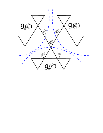
Figure 2: The procedure of derivation of the recursion relation for the partition function on Husimi lattice

Using the hierarchical structure of Husimi lattice one can derive recursion relation for the partition function. The partition function of the system with Hamiltonian (10) is

$$Z=\sum\limits_{\{s_{i}\}}{e^{-H\left(s_{1},s_{2},...s_{n}\right)/k_{B}T}},$$ (12)

where $k_{B}$ is Boltzmann constant, $T$ is temperature and the sum goes over all $\{s_{1},s_{2},...s_{n}\}$ configurations of the system. In the rest of the paper all constants will be taken in Boltzmann constant’s scaling ($\mathrm{J}_{2}/k_{B}\equiv J_{2},\ \mathrm{J}_{3}/k_{B}\equiv J_{3},\ \mathrm{h}/k_{B}\equiv h$). Using Eq. (11) one can write

$$-\frac{H\left(s_{1},s_{2},...s_{n}\right)}{k_{b}T}=-\frac{{J_{2}}}{2\,T}\sum\limits_{\left\langle i,j\right\rangle}{\left({1+s_{i}s_{j}}\right)}+\frac{{J_{3}}}{2\,T}\sum\limits_{\left\langle i,j,k\right\rangle}{\left({1+s_{i}s_{j}+s_{j}s_{k}+s_{k}s_{i}}\right)}+\frac{h}{T}\sum\limits_{i}{s_{i}}.$$ (13)

To obtain recursion relation for the partition function one can separate Husimi lattice into three identical parts (branches) and at first realize summation over all spin configurations on each branch, then to sum over spins of the central triangle. The result of the summation for each branch will only depend on value of corresponding spin variable (see Fig. 2). By denoting

$$\Delta(s_{1},s_{2},s_{3})=-\frac{{J_{2}}}{2\,}\left({3+s_{1}s_{2}+s_{2}s_{3}+s_{3}s_{1}}\right)+\frac{{J_{3}}}{2\,}\left({1+s_{1}s_{2}+s_{2}s_{3}+s_{3}s_{1}}\right),$$ (14)

we can rewrite the expression for the partition function in the following form:

$$Z=\sum\limits_{s^{(0)}_{i}}{exp\left\{\frac{\Delta\left(s^{(0)}_{1},s^{(0)}_{2},s^{(0)}_{3}\right)}{T}+\frac{h\left(s^{(0)}_{1}+s^{(0)}_{2}+s^{(0)}_{3}\right)}{T}\right\}g_{n}(s^{(0)}_{1})g_{n}(s^{(0)}_{2})g_{n}(s^{(0)}_{3})},$$ (15)

where sum goes over central triangle, $g_{n}(s^{(0)}_{i})$ denotes the contribution of a branch at the $s^{(0)}_{i}$-th site of the central triangle and $n$ is number of generations.

At the same way one can express $g_{n}(s^{(0)}_{i})$ in terms of $g_{n-1}(s^{(1)}_{i})$ cutting it along any site of the first generation. Therefore

$$g_{n}(s^{(0)}_{1})=\sum\limits_{s^{(1)}_{2}s^{(1)}_{3}}{exp\left\{\frac{\Delta\left(s^{(0)}_{1},s^{(1)}_{2},s^{(1)}_{3}\right)}{T}+\ \frac{h\left(s^{(1)}_{2}+s^{(1)}_{3}\right)}{T}\right\}g_{n-1}(s^{(1)}_{2})g_{n-1}(s^{(1)}_{3}).}$$ (16)

After the summation we get the following expressions for $g_{n}(s_{i})$

$$g_{n}(+) = e^{\frac{-3J_{2}+2J_{3}+2h}{T}}g_{n-1}^{2}(+)\,\,+\,\,2e^{-\frac{J_{2}}{T}}g_{n-1}(+)g_{n-1}(-)\,\,+\,\,e^{\frac{-J_{2}-2h}{T}}g_{n-1}^{2}(-),$$

$$g_{n}(-) = e^{\frac{-J_{2}+2h}{T}}g_{n-1}^{2}(+)\,\,+\,2e^{-\frac{J_{2}}{T}}g_{n-1}(+)g_{n-1}(-)\,\,+\,\,e^{\frac{-3J_{2}+J_{3}-2h}{T}}g_{n-1}^{2}(-),$$

where we denote $g_{n}(s_{i})$ by $g_{n}(\pm)$ depending on $s_{i}$ sign. By introducing $x_{n}=g_{n}(+)/g_{n}(-)$ variable the recursion relation for the partition function can be obtained

$$x_{n} = f(x_{n-1}),$$

$$f(x) = \frac{1+2cx+ac^{2}x^{2}}{a+2cx+c^{2}x^{2}},$$ (18)

where $a\equiv e^{\frac{2(J_{3}-J_{2})}{T}},\ c\equiv e^{\frac{2h}{T}}$. The thermodynamic functions of the system, such as magnetization, can be expressed in terms of $x_{n}$. The magnetization of the $s^{(0)}_{1}$ site is expressed

$$m=\left\langle s^{(0)}_{1}\right\rangle=\frac{\sum\limits_{\{s_{i}\}}{s^{(0)}_{1}e^{-H\left(s_{1},s_{2},...s_{n}\right)/k_{B}T}}}{\sum\limits_{\{s_{i}\}}{e^{-H\left(s_{1},s_{2},...s_{n}\right)/k_{B}T}}}.$$ (19)

Let us at first realize the summation over central vertex $s_{1}^{(0)}$and then over all other spin variables. After inserting equations (3) into (19) the formula for magnetization will take the following form

$$m=\frac{{e^{\frac{h}{T}}g_{n}^{2}(+)-e^{-\frac{h}{T}}g_{n}^{2}(-)}}{{e^{\frac{h}{T}}g_{n}^{2}(+)+e^{-\frac{h}{T}}g_{n}^{2}(-)}}=\frac{{cx_{n}^{2}-1}}{{cx_{n}^{2}+1}}.$$ (20)

For arbitrary value of magnetic filed $h$, with given temperature and exchange parameters one can draw the dependence of magnetization from external magnetic field by implementing the simple iteration from the recursion relation for $f(x)$, beginning with some initial value of $x_{0}$, The thermodynamic limit correspond to infinite number of iterations $(n\rightarrow\infty)$.

4 The Magnetization and Lyapunov Exponent

In this section the magnetic properties of the model in an external magnetic field have been studied. As known, $J_{2}$ and $J_{3}$ are not obtainable in the experimental measurements, because $n$-spin exchange also makes a contribution to $(n-1)$-spin exchanges, but there is some effective exchange parameter, $J=J_{2}-2J_{3}$ which can be directly obtained from the experiments. The magnetic properties of the model depend on value of effective exchange parameter and vary from ferromagnetic into antiferromagnetic one, depending on whether two- or three-spin exchange interaction is dominant. From experimental measurements and theoretical calculations we know that at low-density region three-site exchange interaction on the regular triangular lattice is dominant. The corresponding estimated value[14] of exchange parameter is $J=J_{2}-2J_{3}=-3.07mK$.

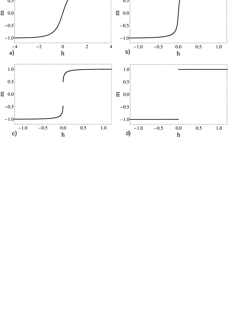
Figure 3: The magnetization curves for $J_{2}=2mK,J_{3}=2.5mK$, $n=50000$ and for (a) $T=1.5mK$, (b) $T=0.7mK$, (c) $T=0.6mK$, (d) $T=0.3mK$

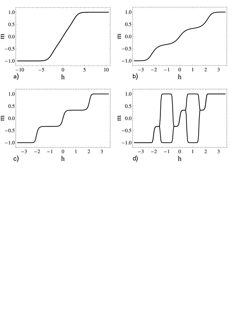
Figure 4: The magnetization curves for $J_{2}=3mK$, $J_{3}=2mK$, $N=50000$ and for (a) $T=1mK$, (b) $T=0.3mK$, (c) $T=0.1mK$, (d) $T=0.05mK$

According to general principles ground state of the system in this case is ferromagnetic. Magnetization function of the model with exchange parameters $J_{2}=2\ mK$ and $J_{3}=2.5\ mK$ is presented in Fig. 3. For high temperatures the magnetization curve has monotone form of Langevin type (Fig. 3(a)). The value of saturation field as large as higher temperature (Fig. 3(b)). For some value temperature (critical temperature) the magnetization curve ceases to be smooth, the jump of magnetization takes place at an arbitrary low value of the applied magnetic field (Fig. 3(c)). The ground state of the model ordered ferromagnetic. The magnetization in zero field is equal to its maximal value, which corresponds to the ferromagnetic phase with all spins pointed in the same direction. Under the effect of an arbitrary weak magnetic field the twofold degeneracy of this phase is removed by orienting all spins along the field. The corresponding diagram is presented in Fig. 3(d).

The model is antiferromagnetic if two-site exchange interaction is dominant. In Fig. 4 are presented magnetization curves that correspond to the values of exchange parameters $J_{2}=3\ mK$ and $J_{3}=2\ mK$. As expected the magnetization curve is of Langevin type for the high temperatures (Fig. 4(a)) and the saturation field decrease with the temperature (Fig. 4(b)). With further decreasing of the temperature plateau at 1/3 of saturation field appears on the magnetization curve (Fig. 4(c)). This phenomena can be explained in the following way. For each triangle two spins directed along magnetic field and the other one oriented opposite to the field (”up-up-down”phase).

At lower temperatures the magnetization plateau turns into bifurcation points and period doubling (Fig. 4(d)). These bifurcation points will disappear if number of iterations tends to infinity. As it is known Lyapunov exponent[54, 55, 56, 57] is exactly zero simultaneously with bifurcation points, indicated in some external parameters and temperature. The Lyapunov exponent is the index of exponential divergence of two near points after $N$ iterations:

$$\varepsilon e^{N\lambda(x_{0})}\approx\left|f^{(N)}(x_{0}+\varepsilon)-f^{(N)}(x_{0})\right|,$$ (21)

where $f^{(N)}(x)=\overbrace{f(f(\ldots f(x)))}^{N}$. In the limit at $\varepsilon\to 0$ and $N\to\infty$ (21) gives the exact formula for $\lambda(x_{0})$

$$\lambda(x_{0})=\mathop{\lim}\limits_{N\to\infty}\mathop{\lim}\limits_{\varepsilon\to 0}\frac{1}{N}\ln\left|{\frac{{f^{(N)}(x_{0}+\varepsilon)-f^{(N)}(x_{0})}}{\varepsilon}}\right|=\mathop{\lim}\limits_{N\to\infty}\frac{1}{N}\ln\left|{\frac{{df^{(N)}(x_{0})}}{{dx_{0}}}}\right|.$$ (22)

Using formula for derivative of composite function

$$\left.{\frac{d}{{dx}}f^{(2)}(x)}\right|_{x_{0}}=f^{\prime}(f(x_{0}))f^{\prime}(x_{0})=f^{\prime}(x_{1})f^{\prime}(x_{0}),\,\,\,x_{1}\equiv f(x_{0}),$$ (23)

one can transform Eq. (22) in the following form

$$\lambda(x_{0})=\mathop{\lim}\limits_{N\to\infty}\frac{1}{N}\ln\left|{\frac{d}{{dx_{0}}}f^{(N)}(x_{0})}\right|=\mathop{\lim}\limits_{N\to\infty}\frac{1}{N}\ln\left|{\prod\limits_{i=0}^{N-1}{f^{\prime}(x_{i})}}\right|.$$ (24)

If Lyapunov exponent is negative, then the final state of the system after iterations tends to stable point of stable cycle composed of more than one points. The positive Lyapunov exponent result in chaotic final state of the system and zero Lyapunov exponent correspond to bifurcation points.

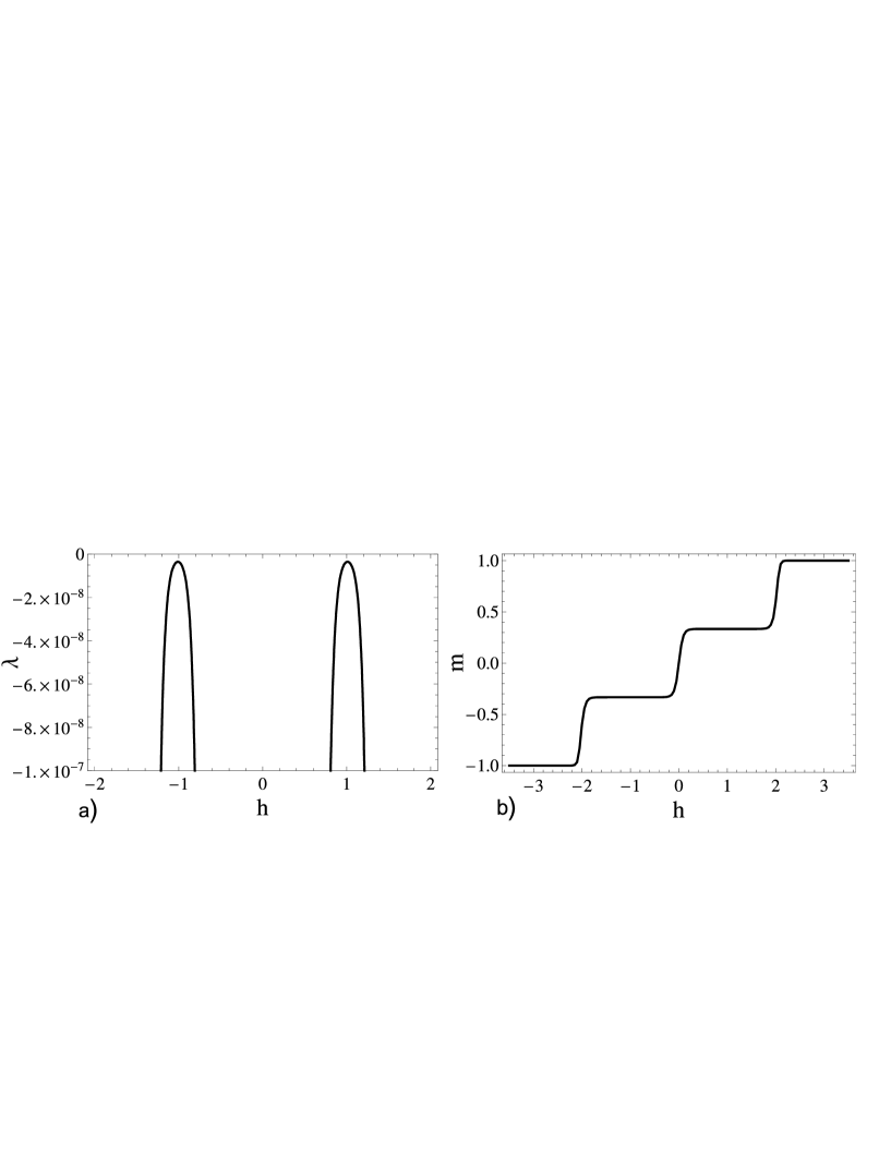
Figure 5: The plots of Lyapunov exponent (a) and magnetization curve (b) for the values of exchange parameters $J_{2}=3mK,J_{3}=2mK,$ temperature $T=0.05mK$ and iterations n=1 500 000 000.

Using Eq. (24) one can plot dependence of Lyapunov exponent from external magnetic field. In Fig. 5(a) Lyapunov exponent curve for $J_{2}=3\ mK$, $J_{3}=2\ mK$ and $T=0.05mK$ has been plotted. Near plateau Lyapunov exponent is very close to zero but it does not cut the axes. In Fig. 5(b) the magnetization curve for the same values of exchange parameters, temperature and number of iterations $n=1\,500\,000\,000$ has been plotted. As can be seen from figure the bifurcation points disappeared.

5 Yang-Lee Zeroes On Husimi lattice

The thermodynamic properties of the system may be investigated by studying the dynamics of the corresponding recursive function (3). As known from dynamical system theory when the number of iterations tends to infinity $(n\rightarrow\infty)$ the resulting point can have different behavior: 1) limiting point tends to one point, 2) limiting point tends to the set of points 3) limiting point has chaotic behavior. In the first case resulting point can tend to one of the stable fixed points. The point $x^{*}$ called fixed point of recursion relation $x_{n}=f(x_{n-1})$ if $x^{*}=f(x^{*})$. The fixed point can be stable (the iterations of any point $x_{0}$ near $x^{*}$ tend to the $x^{*}$), or not stable (the iterations of any point $x_{0}$ near $x^{*}$ tend to move away from $x^{*}$). The stability of fixed point depends on value of the derivative of $f(x)$ at that fixed point $x^{*}$. If $\left|\lambda\right|<1$ where $\lambda\equiv~{}f^{\prime}(x^{*})$ then the fixed point called attracting, if $\left|\lambda\right|>1$ then the fixed point called repelling and if $\left|\lambda\right|=1$ the fixed point called neutral (indifferent). The values of external parameters (temperature, magnetic field, etc.) at which system has only one attracting fixed point correspond to a stable paramagnetic state. If the system has two attracting fixed points then the stable state corresponds to the fixed point with maximum value of $\left|\lambda\right|$, moreover the values of external parameters at which $\left|\lambda_{1}\right|=\left|\lambda_{2}\right|$ correspond to two possible ferromagnetic states with opposite magnetizations.

The fixed points of the recursion relation (3) determined by following equation

$$x=\frac{1+2cx+ac^{2}x^{2}}{a+2cx+c^{2}x^{2}}.$$ (25)

In general this equation has three complex solutions. If there are only one attracting fixed point then the system state is paramagnetic and phase transition does not present. The values of external parameters at which system has two attracting fixed points correspond to metastable region[61]. The boundary of metastable region can be found from the condition that one of the fixed points become neutral. There are not phase transition on the boundary of metastable region. The phase coexistence lines can be found from the condition that absolute values of derivatives at the fixed points become equal[67]. When phase coexistence line cuts the real axis then the system undergoes first order phase transition. The locus of the phase coexistence line inside metastable region correspond to the locus of Yang-Lee zeroes. Consequently, the boundary of metastable region can be determined from the following system of equations:

$$\left\{\begin{array}[]{l}f(x)=x\\ f^{\prime}(x)=e^{i\varphi}\\ \end{array}\right..$$ (26)

Eliminating $x$ from this equations for given temperature and exchange parameters one can find the equation for $c$ parameter.

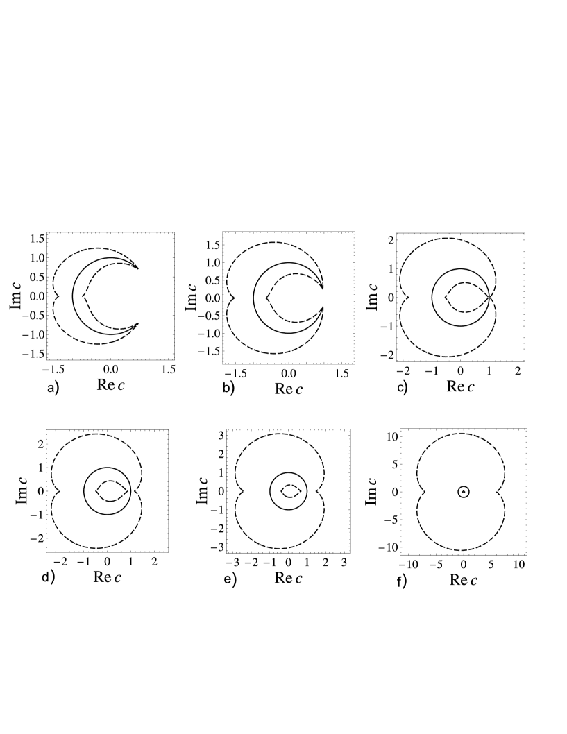
Figure 6: The border of metastable region (dashed curve) and phase coexistence lines (solid curve) for $J_{2}=2mK,J_{3}=2.5mK$ and (a) $T=1.5mK$, (b) $T=0.9mK$, (c) $T=0.6mK$, (d) $T=0.5mK$, (e) $T=0.3mK$, (f) $T=0.1mK$.

In Fig. 6 by dashed line boundary of metastable region for $J=-3mK$ ($J_{2}=2mK,J_{3}=2.5mK$) and different values of temperature are plotted. By solid line phase coexistence lines inside the metastable region are plotted . If $T>T_{c}$ phase coexistence line does not cut the real axes and is an arc of a circle with radius $R=1$ (Fig. 6 (a), (b)). For $T<T_{c}$ phase coexistence line cuts the real axes and the first order phase transitions occurs, therefore system has ferromagnetic behavior (Fig. 6 (c), (d), (e), (f)). Our calculations show that for this values of exchange parameters $T_{c}=1.2426\cdot(J_{3}-J_{2})=0,6213mK.$

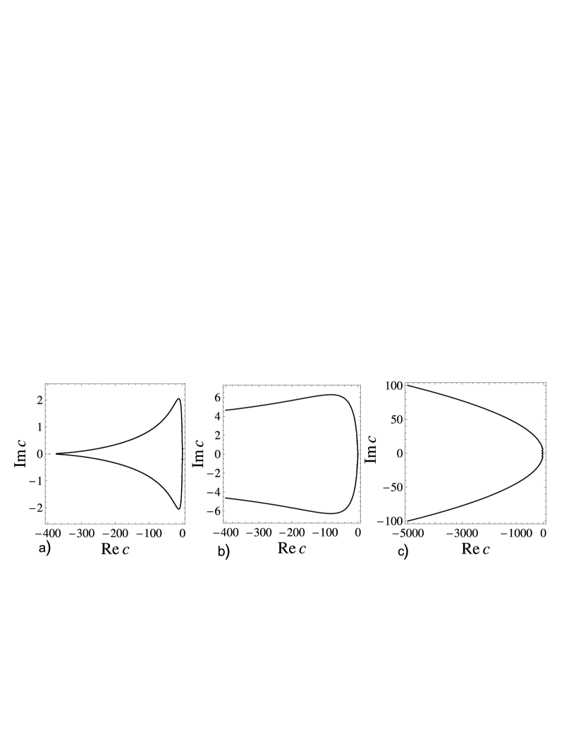
Figure 7: The border of metastable region for $J_{2}=3mK,J_{3}=2mK$ and (a) $T=1mK$, (b) $T=0.5mK$, $T=0.1mK$.

If the two-site exchange interaction is dominant the system has antiferromagnetic behavior. For this case in the metastable region there are two attracting fixed points but they never become equal (no phase coexistence line in the metastable region), therefore Yang-Lee zeroes correspond to the boundary of metastable region. In Figure 7 boundary of metastable region calculated using equation (26) for $J_{2}=3mK,J_{3}=2mK$ and various temperatures are plotted. There is a relation between appearance of plateaus and locus of the Yang-Lee zeroes. The locus of the Yang-Lee zeroes (Fig. 7 (a),(b)) for the values of temperature for which plateau does not appear on magnetization curve (Fig. 4(a),(b)) have been bounded. The locus of Yang-Lee zeroes is unbounded (Fig. 7(c)) if the plateau appear on the magnetization curve (Fig. 4(c)).

6 Conclusions

In the present paper dynamic system theory has been used to study solid and fluid ${}^{3}He$ films absorbed on the surface of graphite. The third layer of ${}^{3}He$ films, which is kagome lattice was approximated by $(\gamma=2)$ Husimi one. In the strong external magnetic field the Ising model have been considered instead of Heisenberg one with two- and three-site exchange interactions. This approach allows us to obtain magnetization curves for different temperatures. The magnetization plateau at 1/3 of saturation field has been obtained for some values of exchange parameters and temperatures. By studying Lyapunov exponent for antiferromagnetic case the absence of the bifurcation points on magnetization plateau at low temperature have been shown.

The Yang-Lee zeroes have been studied in terms of neutral fixed points of the recursion relation. It was shown that Yang-Lee zeroes on the complex $e^{2h/T}$ plane located inside the metastable region (existence of two attracting fixed points) and correspond to phase coexistence lines (the lines where absolute derivatives in fixed points are equal). The locus of the Yang-Lee zeroes for different values of exchange parameters and temperature have been plotted. It was shown that for the ferromagnetic case Yang-Lee zeroes are located on the arc of the unit circle. For antiferromagnetic case if there are magnetization plateaus the locus of Yang-Lee zeroes are infinite, otherwise they are finite.

References

- [1] M. Roger, J. H. Hetherington, J. M. Delrieu, Rev. Mod. Phys. 55, 1 (1983).
- [2] A. M. Dirac, The Principles of Quantum Mechanics (Clarendon, Oxford, 1947).
- [3] H. Franco, R. Rapp, and H. Godfrin, Phys. Rev. Lett. 57, 1161 (1986).
- [4] H. Godfrin, R. Ruel, and D.D. Osheroff, ibid. 60, 305 (1988).
- [5] H. Godfrin and R.E. Rapp, Adv. Phys. 44, 113 (1995).
- [6] E. Collin, S Triqueneaux, R. Harakaly, M. Roger, C. Bäauerle, Yu. M. Bunkov and H. Godfrin, Phys. Rev. Lett. 86, 2447 (2001).
- [7] R. Liebmann, Lecture Notes in Physics (Springer, Berlin, 1986), Vol. 251.
- [8] M.F. Collins and O.A. Petrenko, Can. J. Phys. 75, 605 (1997).
- [9] H. Jichu and K. Kuroda, Prog. Theor. Phys. 67, 715 (1982).
- [10] R. A. Gayer, Phys. Rev. Lett. 64, 1919 (1990).
- [11] M. Roger, Phys. Rev. B. 56, R2928 (1997).
- [12] M. Siquera, J. Nyeki, B. Cowan and J. Saunders, Phys. Rev. Lett. 76, 1884 (1996).
- [13] K. Ishida, M. Morishita, K. Yawata and H. Fukuyama, Phys. Rev. Lett. 79, 3451 (1997).
- [14] M. Roger, C. Bauerle, Yu. M. Bunkov, A. S. Chen and H. Godfrin, Phys. Rev. Lett. 80, 1308 (1998).
- [15] J. M. Delrieu, M. Roger, and J. H. Hetherington, J. Low Temp. Phys. 40, 71 (1980).
- [16] M. Roger, Phys. Rev. B 30, 6432 (1984).
- [17] W. M. Liu, J. L. Song, F. Zhou, Phys. Rev. Lett. 101, 010402 (2008)
- [18] A. C. Ji, 1. A. C. Ji, Q. Sun, X. C. Xie, W. M. Liu, Phys. Rev. Lett. 102, 023602 (2009)
- [19] R. Qi, X. L. Yu, Z. B. Li, W. M. Liu, Phys. Rev. Lett. 102, 185301 (2009)
- [20] J. Davis and R. Packard, Rev. Mod. Phys. 74, 741 (2002)
- [21] J. M. Kosterlitz and D. J. Thouless, J. Phys. C: Solid State Phys. 6 1181-1203 (1973)
- [22] Y. Y. Zhang, J. P. Hu, B. A. Bernevig, X. R. Wang, X. C. Xie, W. M. Liu, Phys. Rev. Lett. 102, 106401 (2009)
- [23] K. Hida, J. Phys. Soc. Jpn. 63, 2359 (1994).
- [24] A. Z. Akheyan, N. S. Ananikian and S. K. Dallakian, Phys. Lett. A 242, 111 (1998); N. S. Ananikian, S. K. Dallakian, N. Sh. Izmailian and K. A. Oganessyan , Phys. Lett. A 214, 205 (1996).
- [25] T. A. Arakelyan, V. R. Ohanyan, L. N. Ananikian, N. S. Ananikian and M. Roger, Phys. Rev. B 67, 024424 (2003).
- [26] V. R. Ohanyan and N. S. Ananikian, Phys. Lett. A 307, 76 (2003).
- [27] L. N. Ananikyan, Int. J. of Mod. Phys. B 21 755 (2007).
- [28] V. V. Hovhannisyan, L. N. Ananikyan, and N. S. Ananikian, Int. J. of Mod. Phys. B 21 3567 (2007).
- [29] V. V. Hovhannisyan and N.S. Ananikian, Phys. Lett. A 372 3363 (2008).
- [30] D. Antonosyan, S. Bellucci, and V. Ohanyan Phys. Rev. B 79, 014432 (2009).
- [31] K. Okamoto, Solid State Commun. 98, 245 (1996).
- [32] T. Tonegawa, T. Nakao, and M. Kaburagi, J. Phys. Soc. Jpn. 65, 3317 (1996).
- [33] K. Totsuka, Phys. Lett. A 228, 103 (1997); Phys. Rev. B 57, 3454 (1998).
- [34] T. Sakai and M. Takahashi, ibid. 57, R3201 (1998).
- [35] G. Japaridze and E. Pogosyan, J. Phys.: Condens. Matter 18, 9297 (2006)
- [36] T. Vekua, G.I. Japaridze, and H. J. Mikeska, Phys. Rev B 67, 064419 (2003).
- [37] H. Suematsu, K. Ohmatsu, K. Sugiyama, T. Sakakibara, M. Motokawa and M. Date, Solid State Commun. 40, 241 (1981).
- [38] T. Sakakibara, K. Sugiyama, M. Date, and H. Suematsu, Synth. Met. 6, 165 (1988).
- [39] H. Nojiri, Y. Tokunaga, and M. Motokawa, J. Phys. (Paris), Colloq. 49, C8-1459 (1988).
- [40] H. Tanaka, W. Shiramura, T. Takatsu, B. Kurniawan, M. Takahashi, K. Kamishima, K. Takizawa, H. Mitamura and T. Goto, Physica B, 230, 246 (1998).
- [41] H. Kageyama, K. Yoshimura, R. Stern, N. V. Mushnikov, K.Onizuka, M. Kato, K. Kosuge, C. P. Slichter, T. Goto and Y. Ueda, Phys. Rev. Lett., 82, 3168 (1999).
- [42] S. Miyahara and K. Ueda, Phys. Rev. Lett., 82 3701 (1999).
- [43] E. Müller-Hartmann, R. R. P. Singh, C. Knetter and G. S. Uhrig, Phys. Rev. Lett., 84, 1808 (2000).
- [44] K. Totsuka, S. Miyahara and K. Ueda, Phys. Rev. Lett., 86, 520 (2001).
- [45] G. Misguich, T. Jolicoeur and S. M. Girvin, Phys. Rev. Lett., 87,097203 (2001).
- [46] K. Kodama, M. Takigawa, M. Horvatić, C. Berthier, H. Kageyama, Y. Ueda, S. Miyahara, F. Becca and F. Mila, Science, 298, 395 (2002).
- [47] Y. Narumi, K. Katsumata, Z. Honda, J. C. Domenge, P. Sindzingre, C. Lhuillier, Y. Shimaoka, T. C. Kobayashi and K. Kindo, Europhys. Lett., 65 (5), pp.705-711 (2004).
- [48] H. Yoshida, Y. Okamoto, T. Tayama, T. Sakakibara, M. Tokunaga, A. Matsuo, Y. Narumi, K. Kindo, M. Yoshida, M. Takigawa and Z. Hiroi, J. Phys. Soc. Jpn. 78, 043704 (2009).
- [49] M. Oshikawa, M. Yamanaka, and I. Affleck, Phys. Rev. Lett. 78, 1984 (1997).
- [50] C. Zeng and V. Elser, Phys. Rev. B 51, 8318 (1995).
- [51] P. W. Leung and V. Elser, Phys. Rev. B 47, 5459 (1993).
- [52] Ch. Waldtmann et al., Eur. Phys. J. B 2, 501 (1998).
- [53] R. Baxter, Exactly Solved Models in Statistical Mechanics (Academic Press, New York, (1982), Chap. 4).
- [54] V. I. Oseledec, Trans. Moskow Math. Soc. 19, 197 (1968).
- [55] J. P. Eckmann and D. Ruelle, Rev. Mod. Phys. 57, 617 (1985).
- [56] . Birol and A. Hacinliyan, Phys. Rev. E 52, 4750 (1995).
- [57] G. Casati, B. V. Chirikov, Quantum chaos: between order and disorder (Cambridge University Press, 1995).
- [58] T. D. Lee and C. N. Yang, Phys. Rev. 87: 404 (1952).
- [59] T. D. Lee and C. N. Yang, Phys. Rev. 87: 410 (1952).
- [60] R. G. Ghulghazaryan and N. S. Ananikian, J. Phys. A: Math. Gen. 36, 6297 (2003),
- [61] R. G. Ghulghazaryan, N. S. Ananikian and P. M. A. Sloot, Phys. Rev. E. 66, 046110 (2002).
- [62] N. S. Ananikian, R. G. Ghulghazaryan, Phys. Lett. A 277, 249 (2000).
- [63] S. Y. Kim and R. Creswick, Phys. Rev. Lett. 81, 2000 (1998); Phys. Rev. E 58, 7006 (1998).
- [64] R. Creswick and S. Y. Kim, Physica A 281, 252 (2000).
- [65] S. Y. Kim, R. Creswick, C. N. Chen, and C. K. Hu, Physica A 281, 262 (2000).
- [66] C. N. Chen, C. K. Hu, and F. Y. Wu, Phys. Rev. Lett. 76, 169 (1996).
- [67] M. Biskup, C. Borgs, J. T. Chayes, L. J. Kleinwaks, and R. Kotecky, Phys. Rev. Lett. 84, 4794 (2000).
- [68] J. L. Monroe, Phys. Lett. A 188, 80 (1994).