Multigraded Commutative Algebra of Graph Decompositions

Abstract.

The toric fiber product is a general procedure for gluing two ideals, homogeneous with respect to the same multigrading, to produce a new homogeneous ideal. Toric fiber products generalize familiar constructions in commutative algebra like adding monomial ideals and the Segre product. We describe how to obtain generating sets of toric fiber products in non-zero codimension and discuss persistence of normality and primary decompositions under toric fiber products.

Several applications are discussed, including (a) the construction of Markov bases of hierarchical models in many new cases, (b) a new proof of the quartic generation of binary graph models associated to $K_{4}$-minor free graphs, and (c) the recursive computation of primary decompositions of conditional independence ideals.

1. Introduction

Let $I$ and $J$ be ideals in polynomial rings $\mathbb{K}[x]$ and $\mathbb{K}[y]$, respectively, that are both homogeneous with respect to a single grading by an affine semigroup $\mathbb{N}\mathcal{A}$. The toric fiber product of $I$ and $J$ (Definition 2.1), denoted $I\times_{\mathcal{A}}J,$ is a new ideal in a usually larger polynomial ring $\mathbb{K}[z]$. An important measure of complexity of this operation is the codimension of the product, defined as the rank of the integer lattice $\ker\mathcal{A}$. In [34] the third author introduced toric fiber products and proved that in the codimension zero case it is possible to construct a generating set or Gröbner basis for $I\times_{\mathcal{A}}J$ from generating sets or Gröbner bases of $I$ and $J$. In this case the algebra and geometry is significantly simpler essentially because codimension zero toric fiber products are multigraded Segre products (Definition 2.3), which share many nice properties with their standard graded analogues. Still in the codimension zero case, the geometry of the toric fiber product can be understood quite explicitly in terms of GIT [25] (Propositions 2.2 and 2.4). We pursue this observation and show that (under mild assumptions on $\mathbb{K}$) normality persists (Theorem 2.5).

The main goal of this paper, however, is to describe higher codimension toric fiber products. In Section 3 we show that primary decompositions persist in any codimension (Theorem 3.1). In Section 4 we show how to construct generating sets of toric fiber products in arbitrary codimension, but under some extra technical conditions (Theorem 4.9). This generalizes the codimension one results on cut ideals obtained by the first author in [11].

The toric fiber product frequently appears in applications of combinatorial commutative algebra, in particular in algebraic statistics [12, 31, 32]. Typically in algebraic statistics, we are interested in studying a family of ideals, where each ideal $I_{G}$ is associated to a graph $G$ (or other combinatorial object, like a simplicial complex or a poset). If the graph has a decomposition into two simpler graphs $G_{1}$ and $G_{2}$, we would like to show that the ideal $I_{G}$ has a decomposition into the two ideals $I_{G_{1}}$ and $I_{G_{2}}$. If we can identify $I_{G}$ as a toric fiber product $I_{G_{1}}\times_{\mathcal{A}}I_{G_{2}}$, then difficult algebraic questions for large graphs reduce to simpler problems on smaller graphs. Our inspiration comes from structural graph theory, where the imposition of forbidden substructures often implies that a graph has a specific kind of structural decomposition into simple pieces. In Section 5 we pursue the analogy to the theory of forbidden minors [29] by exhibiting minor-closed classes of graphs with certain degree bounds on their Markov bases.

Before proving our main theoretical results in Sections 2–4, we motivate our study with several examples from algebraic statistics. Sections 5 and 6 contain new applications to the construction of Markov bases of hierarchical models, and to the study of primary decompositions of conditional independence ideals.

1.1. Hierarchical models

Hierarchical statistical models are used to analyze associations between collections of random variables. If the random variables are discrete, these models are toric varieties, and hence their vanishing ideals are toric ideals. Their binomial generators—known as Markov bases—are useful for performing various tests in statistics [6, 10]. From the algebraic standpoint, they are binomial ideals with a specific combinatorial parametrization in terms of a simplicial complex.

Let $\Gamma\subseteq 2^{V}$ be a simplicial complex on a finite set $V$ and $d\in\mathbb{Z}^{V}_{\geq 2}$. Let ${\rm facet}(\Gamma)$ be the set of maximal faces of $\Gamma$. For an integer $n$, let $[n]=\{1,2,\ldots,n\}$. For $F\subseteq V$ let $d_{F}=(d_{v})_{v\in F}$ and let $\mathrm{D}_{F}=\prod_{v\in F}[d_{v}]$. For $i\in\mathrm{D}_{V}$ and $F\subseteq V$ let $i_{F}=(i_{v})_{v\in F}$ be the restriction. For each $F\in{\rm facet}(\Gamma)$ and $i\in\mathrm{D}_{F}$, let $a^{F}_{i}$ be an indeterminate. For each $i\in\mathrm{D}_{V}$, let $p_{i}$ be another indeterminate. The toric ideal $I_{\Gamma,d}$ of the hierarchical model for $(\Gamma,d)$ is the kernel of the $\mathbb{K}$-algebra homomorphism

$$\phi_{\Gamma,d}:\mathbb{K}[p_{i}:i\in\mathrm{D}_{V}]\rightarrow\mathbb{K}[a^{F}_{j}:F\in{\rm facet}(\Gamma),j\in\mathrm{D}_{F}]\qquad p_{i}\mapsto\prod_{F\in{\rm facet}(\Gamma)}a^{F}_{i_{F}}.$$

A fundamental problem of algebraic statistics is to determine generators for $I_{\Gamma,d}$. Results in this direction usually depend on special properties of $\Gamma$ and $d$. An example is the following theorem of Král, Norine, and Pangrác [21], which is also a corollary to our results in Section 5.3:

Theorem 1.1.

Let $d_{i}=2$ for all $i\in V$ and let $\Gamma$ be a graph with no $K_{4}$ minors. Then $I_{\Gamma,d}$ is generated by binomials of degrees two and four.

Combining our techniques with results from [15], we can also make statements about the asymptotic behavior as the $d_{i}$ grow. For instance, let $F\subseteq V$ be an independent set of $\Gamma$ and consider $I_{\Gamma,d}$ as $d_{i}$ tend to infinity for $i\in F$, while the remaining $d_{i}$ are fixed. In this case, there is a bound $M(\Gamma,d_{V\setminus F})$ for the degrees of elements in minimal generating sets of $I_{\Gamma,d}$. Our techniques allow us to determine the values of $M(\Gamma,d_{V\setminus F})$, which were previously known only for reducible models or when $F$ is a singleton [17]. Here is a simple example of how to apply Theorem 5.15.

Example 1.2.

Let $\Gamma=[12][13][24][34]$ be a four cycle, $F=\{1,4\}$, and $d_{\{2,3\}}=(2,2)$. The toric ideal $I_{\Gamma,d}$ is a codimension one toric fiber product and its minimal generating set consists of the following four types of binomials, written in tableau notation (a common notation, explained below Theorem 4.2):

$$\begin{bmatrix}i_{1}&2&2&l_{1}\\ i_{1}&1&1&l_{2}\\ i_{2}&2&1&l_{3}\\ i_{2}&1&2&l_{4}\end{bmatrix}-\begin{bmatrix}i_{1}&2&1&l_{3}\\ i_{1}&1&2&l_{4}\\ i_{2}&2&2&l_{1}\\ i_{2}&1&1&l_{2}\end{bmatrix}\quad\quad\quad\quad\begin{bmatrix}i_{1}&2&2&l_{1}\\ i_{2}&1&1&l_{1}\\ i_{3}&2&1&l_{2}\\ i_{4}&1&2&l_{2}\end{bmatrix}-\begin{bmatrix}i_{3}&2&1&l_{1}\\ i_{4}&1&2&l_{1}\\ i_{1}&2&2&l_{2}\\ i_{2}&1&1&l_{2}\end{bmatrix}$$

$$\begin{bmatrix}i_{1}&j&k&l_{1}\\ i_{2}&j&k&l_{2}\end{bmatrix}-\begin{bmatrix}i_{1}&j&k&l_{2}\\ i_{2}&j&k&l_{1}\end{bmatrix}\quad\quad\quad\quad\begin{bmatrix}i&2&2&l\\ i&1&1&l\end{bmatrix}-\begin{bmatrix}i&2&1&l\\ i&1&2&l\end{bmatrix}$$

where $i,i_{1},i_{2},i_{3},i_{4}\in[d_{1}]$, $j,k\in[2]$, $l,l_{1},l_{2},l_{3},l_{4}\in[d_{4}]$. In particular, $M(\Gamma,d_{V\setminus F})=4$.

1.2. Conditional independence

If $G$ is a graph on $V$, then its clique complex defines a hierarchical model as in the previous section. Probability distributions in this hierarchical model satisfy certain conditional independence statements associated to the graph [22]. One may ask which other distributions outside the hierarchical model also satisfy the conditional independence constraints, and algebraic statistics allows one to characterize these distributions. Consider again the polynomial ring $\mathbb{K}[p_{i}:i\in\mathrm{D}_{V}]$ with one indeterminate for each elementary probability. If $A,B,C\subset V$ is a partition of $V$, i.e. pairwise disjoint with $A\cup B\cup C=V$, the conditional independence (CI)-statement $\left.A\mathchoice{\mathrel{\hbox to0.0pt{$\displaystyle\perp$\hss}\mkern 2.0mu{\displaystyle\perp}}}{\mathrel{\hbox to0.0pt{$\textstyle\perp$\hss}\mkern 2.0mu{\textstyle\perp}}}{\mathrel{\hbox to0.0pt{$\scriptstyle\perp$\hss}\mkern 2.0mu{\scriptstyle\perp}}}{\mathrel{\hbox to0.0pt{$\scriptscriptstyle\perp$\hss}\mkern 2.0mu{\scriptscriptstyle\perp}}}B\,\middle|C\right.{}$ encodes that the random variables in $A$ are independent of the random variables in $B$, given the values of the random variables in $C$. Distributions satisfying this constraint form a hierarchical model, which arises from the largest simplicial complex on $V$ not containing $\left\{i,j\right\}$ for any $i\in A,j\in B$. Its toric ideal is denoted $I_{\left.A\mathchoice{\mathrel{\hbox to0.0pt{$\displaystyle\perp$\hss}\mkern 2.0mu{\displaystyle\perp}}}{\mathrel{\hbox to0.0pt{$\textstyle\perp$\hss}\mkern 2.0mu{\textstyle\perp}}}{\mathrel{\hbox to0.0pt{$\scriptstyle\perp$\hss}\mkern 2.0mu{\scriptstyle\perp}}}{\mathrel{\hbox to0.0pt{$\scriptscriptstyle\perp$\hss}\mkern 2.0mu{\scriptscriptstyle\perp}}}B\,\middle|C\right.{}}$. A conditional independence model usually contains several statements and one is led to consider intersections of toric varieties. Our main interest is in the global Markov ideal of a graph $G$, which is the sum of the toric ideals $I_{\left.A\mathchoice{\mathrel{\hbox to0.0pt{$\displaystyle\perp$\hss}\mkern 2.0mu{\displaystyle\perp}}}{\mathrel{\hbox to0.0pt{$\textstyle\perp$\hss}\mkern 2.0mu{\textstyle\perp}}}{\mathrel{\hbox to0.0pt{$\scriptstyle\perp$\hss}\mkern 2.0mu{\scriptstyle\perp}}}{\mathrel{\hbox to0.0pt{$\scriptscriptstyle\perp$\hss}\mkern 2.0mu{\scriptscriptstyle\perp}}}B\,\middle|C\right.{}}$ for all $A,B,C$ forming a partition of $V$ such that $C$ separates $A$ and $B$ in $G$. Our goal is to determine primary decompositions and as always we want to employ the toric fiber product machinery to split the problem into several easier problems.

Example 1.3.

Let $G$ be the binary global Markov ideal of the graph in Figure 1.

Figure 1. Three squares glued along edges

Since it decomposes as three squares glued along edges, Theorem 3.1 and Corollary 3.2 reconstruct the primary decomposition from that of the CI-ideal of a square. Our results also show that the corresponding CI-ideal is radical, as it is composed of graphs with radical CI-ideals. In total it is the intersection of $729=9^{3}$ prime ideals.

A systematic check of all graphs with at most five vertices and with $d_{v}=2$ for all $v\in V$ found no examples of a non-radical global Markov ideal. This limited computational evidence motivates the following question:

Question 1.4.

Are global Markov ideals always radical?

The answer to this question is negative. More than a year after first submission of the present paper, Kahle, Rauh, and Sullivant showed that the global Markov ideal of $K_{3,3}$ is not radical [20].

2. Toric fiber products and multigraded Segre products

Let $r>0$ be a positive integer and $s,t\in\mathbb{Z}^{r}_{>0}$ be two vectors of positive integers. Let

$$\mathbb{K}[x]=\mathbb{K}[x^{i}_{j}:i\in[r],j\in[s_{i}]]\quad\quad\mbox{ and }\quad\quad\mathbb{K}[y]=\mathbb{K}[y^{i}_{k}:i\in[r],k\in[t_{i}]]$$

be multigraded polynomial rings subject to a multigrading

$$\deg(x^{i}_{j})=\deg(y^{i}_{k})=\mathbf{a}^{i}\in\mathbb{Z}^{d}.$$

We assume throughout that there exists a vector $\omega\in\mathbb{Q}^{d}$ such that $\omega^{T}\mathbf{a}^{i}=1$ for all $i$. This implies that ideals homogeneous with respect to the multigrading are homogeneous with respect to the standard coarse grading. Let $\mathcal{A}=\{\mathbf{a}^{1},\ldots,\mathbf{a}^{r}\}$ and let $\mathbb{N}\mathcal{A}$ be the affine semigroup generated by $\mathcal{A}$. If $I\subset\mathbb{K}[x]$ and $J\subset\mathbb{K}[y]$ are $\mathbb{N}\mathcal{A}$-graded ideals, the quotient rings $R=\mathbb{K}[x]/I$ and $S=\mathbb{K}[y]/J$ are also $\mathbb{N}\mathcal{A}$-graded. Let

$$\mathbb{K}[z]=\mathbb{K}[z^{i}_{jk}:i\in[r],j\in[s_{i}],k\in[t_{i}]]$$

and let $\phi_{I,J}:\mathbb{K}[z]\rightarrow R\otimes_{\mathbb{K}}S$ be the $\mathbb{K}$-algebra homomorphism such that $z^{i}_{jk}\mapsto x^{i}_{j}\otimes y^{i}_{k}.$

Definition 2.1.

The toric fiber product $I\times_{\mathcal{A}}J$ of $I$ and $J$ is the kernel of $\phi_{I,J}$:

$$I\times_{\mathcal{A}}J=\ker\phi_{I,J}.$$

The codimension of the toric fiber product is the dimension of the space of linear relations among $\mathcal{A}$.

We can also define the $\mathbb{K}$-algebra homomorphism $\phi:\mathbb{K}[z]\rightarrow\mathbb{K}[x]\otimes_{\mathbb{K}}\mathbb{K}[y]=\mathbb{K}[x,y]$ by $z^{i}_{jk}\mapsto x^{i}_{j}y^{i}_{k}$. Then the toric fiber product is the ideal $I\times_{\mathcal{A}}J=\phi^{-1}(I+J)$.

2.1. The geometry of toric fiber products

If $I\times_{\mathcal{A}}J$ is a codimension zero toric fiber product, the relation between the schemes $\mathrm{Spec}\,(\mathbb{K}[x]/I)$, $\mathrm{Spec}\,(\mathbb{K}[y]/J)$ and $\mathrm{Spec}\,(\mathbb{K}[z]/(I\times_{\mathcal{A}}J))$ can be explained in the language of GIT (geometric invariant theory) quotients. Since $I$ and $J$ are homogeneous with respect to the grading by $\mathcal{A}$, both $\mathrm{Spec}\,(\mathbb{K}[x]/I)$ and $\mathrm{Spec}\,(\mathbb{K}[y]/J)$ have an action of a $(\dim\mathcal{A}-1)$-dimensional torus $T$. Thus the product scheme $\mathrm{Spec}\,(\mathbb{K}[x]/I)\times\mathrm{Spec}\,(\mathbb{K}[y]/J)$ possesses an action of $T$ via $t\cdot(x,y)=(tx,t^{-1}y)$.

Proposition 2.2.

If $\mathbb{K}$ is algebraically closed and $\mathcal{A}$ is linearly independent, then

$$\mathrm{Spec}\,(\mathbb{K}[z]/(I\times_{\mathcal{A}}J))\cong\left(\mathrm{Spec}\,(\mathbb{K}[x]/I)\times\mathrm{Spec}\,(\mathbb{K}[y]/J)\right)//T.$$

Proof.

If $\mathbb{K}$ is algebraically closed, then

$$\mathrm{Spec}\,(\mathbb{K}[x]/I)\times\mathrm{Spec}\,(\mathbb{K}[y]/J)=\mathrm{Spec}\,(\mathbb{K}[x]/I\otimes_{\mathbb{K}}\mathbb{K}[y]/J).$$

Let $R=\mathbb{K}[x]/I$ and $S=\mathbb{K}[x]/J$. Both $R$ and $S$ are $\mathbb{N}\mathcal{A}$-graded, so we can write $R=\oplus_{\mathbf{a}\in\mathbb{N}\mathcal{A}}R_{\mathbf{a}}$, $S=\oplus_{\mathbf{a}\in\mathbb{N}\mathcal{A}}S_{\mathbf{a}}$, and

$$\mathbb{K}[x]/I\otimes_{\mathbb{K}}\mathbb{K}[y]/J=\oplus_{\mathbf{a}\in\mathbb{N}\mathcal{A},\mathbf{b}\in\mathbb{N}\mathcal{A}}R_{\mathbf{a}}\otimes_{\mathbb{K}}S_{\mathbf{b}},$$

where the $\mathbb{Z}\mathcal{A}$ degree of $R_{\mathbf{a}}\otimes_{\mathbb{K}}S_{\mathbf{b}}$ is $\mathbf{a}-\mathbf{b}$. The invariant ring of the torus action is the degree ${\bf 0}$ part, which is $\oplus_{\mathbf{a}\in\mathbb{N}\mathcal{A}}R_{\mathbf{a}}\otimes_{\mathbb{K}}S_{\mathbf{a}}$. The proof is complete once we show that

(1) $$\mathbb{K}[z]/(I\times_{\mathcal{A}}J)\cong\oplus_{\mathbf{a}\in\mathbb{N}\mathcal{A}}R_{\mathbf{a}}\otimes_{\mathbb{K}}S_{\mathbf{a}},$$

since then the spectra must be the same. The toric fiber product $I\times_{\mathcal{A}}J$ is the kernel of the ring homomorphism

$$\phi:\mathbb{K}[z]\rightarrow R\otimes_{\mathbb{K}}S,\quad\quad z^{i}_{jk}\rightarrow x^{i}_{j}\otimes y^{i}_{k},$$

thus the first isomorphism theorem asserts $\mathbb{K}[z]/(I\times_{\mathcal{A}}J)\cong\operatorname{im}\phi$. Since $\deg(x^{i}_{j})=\deg(y^{i}_{k})=\mathbf{a}_{i}$, $\operatorname{im}\phi$ is a subalgebra of $\oplus_{\mathbf{a}\in\mathbb{N}\mathcal{A}}R_{\mathbf{a}}\otimes_{\mathbb{K}}S_{\mathbf{a}}$. We need to show that $\phi$ surjects onto it. As algebras, $R$ is generated by $\oplus_{\mathbf{a}\in\mathcal{A}}R_{\mathbf{a}}$ and $S$ is generated by $\oplus_{\mathbf{a}\in\mathcal{A}}S_{\mathbf{a}}$. Now let $x^{\mathbf{u}}\otimes y^{\mathbf{v}}$ be a monomial in some $R_{\mathbf{a}}\otimes_{\mathbb{K}}S_{\mathbf{a}}$. Since $\mathcal{A}=\{\mathbf{a}_{1},\ldots,\mathbf{a}_{n}\}$ is linearly independent, there is a unique way to write $\mathbf{a}=\sum_{i=1}^{n}\lambda_{i}\mathbf{a}_{i}$ with $\lambda_{i}\in\mathbb{N}$. Thus

$$x^{\mathbf{u}}=\prod_{r=1}^{\lambda_{1}}x^{1}_{j_{1r}}\cdots\prod_{r=1}^{\lambda_{n}}x^{n}_{j_{nr}}\quad\text{ and }\quad y^{\mathbf{v}}=\prod_{r=1}^{\lambda_{1}}y^{1}_{k_{1r}}\cdots\prod_{r=1}^{\lambda_{n}}y^{n}_{k_{nr}}.$$

So we have

$$x^{\mathbf{u}}\otimes y^{\mathbf{v}}=\prod_{r=1}^{\lambda_{1}}x^{1}_{j_{1r}}\otimes y^{1}_{k_{1r}}\cdots\prod_{r=1}^{\lambda_{n}}x^{n}_{j_{nr}}\otimes y^{n}_{k_{nr}}$$

and this monomial is in the subring generated by $\oplus_{\mathbf{a}\in\mathcal{A}}R_{\mathbf{a}}\otimes_{\mathbb{K}}S_{\mathbf{a}}$. Since the monomials span the entire ring $\oplus_{\mathbf{a}\in\mathbb{N}\mathcal{A}}R_{\mathbf{a}}\otimes_{\mathbb{K}}S_{\mathbf{a}}$ as a vector space, every element in $\oplus_{\mathbf{a}\in\mathbb{N}\mathcal{A}}R_{\mathbf{a}}\otimes_{\mathbb{K}}S_{\mathbf{a}}$ is in $\operatorname{im}\phi\cong\mathbb{K}[z]/(I\times_{\mathcal{A}}J)$, which completes the proof. ∎

The assumption of linear independence is essential for the proof of Proposition 2.2 and the statement is no longer true if $\mathcal{A}$ is linearly dependent. We always have

$$\left(\mathrm{Spec}\,(\mathbb{K}[x]/I)\times\mathrm{Spec}\,(\mathbb{K}[y]/J)\right)//T=\mathrm{Spec}\,(\bigoplus_{\mathbf{a}\in\mathbb{N}\mathcal{A}}R_{\mathbf{a}}\otimes_{\mathbb{K}}S_{\mathbf{a}})$$

but (1) fails. Indeed, $\mathbb{K}[z]/(I\times_{\mathcal{A}}J)$ is a strict subset of $\oplus_{\mathbf{a}\in\mathbb{N}\mathcal{A}}R_{\mathbf{a}}\otimes_{\mathbb{K}}S_{\mathbf{a}}$ when $\mathcal{A}$ is linearly dependent. While not, in general, a toric fiber product, this ring and the associated GIT quotient do arise in algebraic geometry, in particular in the work of Buczynska [3] and Manon [23]. Because of its appearance in other contexts, we feel that this object is worthy of its own definition.

Definition 2.3.

Let $R$ and $S$ be two rings graded by a common semigroup $\mathbb{N}\mathcal{A}$. The multigraded Segre product is

$$R\times_{\mathbb{N}\mathcal{A}}S=\oplus_{\mathbf{a}\in\mathbb{N}\mathcal{A}}R_{\mathbf{a}}\otimes_{\mathbb{K}}S_{\mathbf{a}}.$$

With this new definition, Proposition 2.2 is equivalent to the statement:

Proposition 2.4.

If $\mathcal{A}$ is linearly independent, then

$$\mathbb{K}[x]/I\times_{\mathbb{N}\mathcal{A}}\mathbb{K}[y]/J\cong\mathbb{K}[z]/(I\times_{\mathcal{A}}J).$$

2.2. Persistence of normality

One of the most basic questions about an ideal $I$ in a ring $R$ is whether or not the quotient $R/I$ is normal. When $I$ is a toric ideal, $\mathbb{K}[x]/I$ is an affine semigroup ring and normality can be characterized in terms of the semigroup having no holes. In algebraic statistics, normality implies favorable properties of sampling algorithms for contingency tables [4, 36]. In this section we show that normality persists under codimension zero toric fiber products. We only treat the case of (not necessarily toric) prime ideals, which suffices in many situations (see for instance [35, Proposition 2.1.16]).

Theorem 2.5.

Let $I$ and $J$ be homogeneous prime $\mathbb{N}\mathcal{A}$-graded ideals, with $\mathcal{A}$ linearly independent, and suppose that $\mathbb{K}[x]/I$ and $\mathbb{K}[y]/J$ are normal domains (that is, integrally closed in their field of fractions). If $\mathbb{K}$ is algebraically closed, then $\mathbb{K}[z]/(I\times_{\mathcal{A}}J)$ is normal.

The assumption that $\mathbb{K}$ is algebraically closed is needed to ensure that $\mathbb{K}[z]/(I\times_{\mathcal{A}}J)$ is a domain. This holds more generally if $I$ and $J$ are geometrically prime (see Theorem 3.1). If this is given, the field assumption can be weakened to $\mathbb{K}$ being a perfect field, that is a field $\mathbb{K}$ such that either $\operatorname{char}(\mathbb{K})=0$ or $\operatorname{char}(\mathbb{K})=p$ and $\mathbb{K}=\left\{a^{p}:a\in\mathbb{K}\right\}$. The proof of Theorem 2.5 is based on the following observation which is easy and independent of the codimension of $\mathcal{A}$.

Lemma 2.6.

The multigraded Segre product is a direct summand of the tensor product $R\otimes_{\mathbb{K}}S$ (as a module over the subring).

Proof.

The inclusion $0\to\bigoplus_{a\in\mathbb{N}\mathcal{A}}R_{a}\otimes_{\mathbb{K}}S_{a}\to\bigoplus_{a\in\mathbb{N}\mathcal{A}}\bigoplus_{b\in\mathbb{N}\mathcal{A}}R_{a}\otimes_{\mathbb{K}}S_{b}$ splits via the $(\bigoplus_{a\in\mathbb{N}\mathcal{A}}R_{a}\otimes_{\mathbb{K}}S_{a})$-module homomorphism that maps $x^{i}_{j}\otimes y^{l}_{k}$ to itself if $\mathbf{a}_{i}=\mathbf{a}_{l}$ and zero otherwise. ∎

We anticipate that Lemma 2.6 will be useful in relating properties of multigraded Segre products to those of the factors. For instance, a careful analysis of the Castelnuovo–Mumford regularity would be interesting, but is beyond the scope of this paper. We apply the lemma to prove persistence of normality in codimension zero. Note that the codimension requirement enters because only if $\mathcal{A}$ is linearly independent, Lemma 2.6 gives us a handle on the toric fiber product.

Proof of Theorem 2.5.

Let $R=\mathbb{K}[x]/I$ and $S=\mathbb{K}[y]/J$. It is easy to see directly (and also follows from Theorem 3.1 below) that $\mathbb{K}[z]/(I\times_{\mathcal{A}}J)$ is a domain, given that $\mathbb{K}$ is algebraically closed. An algebraically closed field is perfect and therefore, if $R$ and $S$ are normal, then $R\otimes_{\mathbb{K}}S$ is normal. This follows from Serre’s criterion and [38, Theorem 6]. Since a direct summand of a normal domain is normal, Lemma 2.6 completes the proof. ∎

The main case of interest for our applications is when the ideals $I$ and $J$ are toric ideals and various special cases have been proved in the algebraic statistics literature. For example, Ohsugi [27] proves this for cut ideals, Sullivant [33] for hierarchical models, and Michałek [24] for group-based phylogenetic models. The proofs of these results are essentially the same, and consists of analyzing a toric fiber product of the grading semigroup. We introduce this setting now.

2.3. Fiber products of vector configurations

If $I$ and $J$ are toric ideals, then $I\times_{\mathcal{A}}J$ is also a toric ideal. The corresponding vector configuration arises from taking the fiber product of the two vector configurations corresponding to $I$ and $J$. Let $\mathcal{B}=\{\mathbf{b}^{i}_{j}:i\in[r],j\in[s_{i}]\}\subseteq\mathbb{Z}^{d_{1}}$ and $\mathcal{C}=\{\mathbf{c}^{i}_{k}:i\in[r],k\in[t_{i}]\}\subseteq\mathbb{Z}^{d_{2}}$ be two vector configurations. As necessary, we consider $\mathcal{B}$ and $\mathcal{C}$ as collections of vectors or as matrices. These vector configurations define toric ideals $I_{\mathcal{B}}\subseteq\mathbb{K}[x]$ and $I_{\mathcal{C}}\subseteq\mathbb{K}[y]$ by

$$I_{\mathcal{B}}=\left\langle x^{\mathbf{u}}-x^{\mathbf{v}}:\mathcal{B}\mathbf{u}=\mathcal{B}\mathbf{v}\right\rangle\qquad\text{ and }\qquad I_{\mathcal{C}}=\left\langle y^{\mathbf{u}}-y^{\mathbf{v}}:\mathcal{C}\mathbf{u}=\mathcal{C}\mathbf{v}\right\rangle.$$

To say that $I_{\mathcal{B}}$ and $I_{\mathcal{C}}$ are homogeneous with respect to the grading by $\mathcal{A}$ with $\deg(x^{i}_{j})=\deg(y^{i}_{k})=\mathbf{a}^{i}$ is to say that there are linear maps $\pi_{1}:\mathbb{Z}^{d_{1}}\rightarrow\mathbb{Z}^{e}$ and $\pi_{2}:\mathbb{Z}^{d_{2}}\rightarrow\mathbb{Z}^{e}$ such that $\pi_{1}(\mathbf{b}^{i}_{j})=\mathbf{a}^{i}$ for all $i$ and $j$ and $\pi_{2}(\mathbf{c}^{i}_{k})=\mathbf{a}^{i}$ for all $i$ and $k$. The new vector configuration that arises in this case is the fiber product of the vector configurations.

$$\mathcal{B}\times_{\mathcal{A}}\mathcal{C}=\{(\mathbf{b}^{i}_{j},\mathbf{c}^{i}_{k})\in\mathbb{Z}^{d_{1}+d_{2}}:i\in[r],j\in[s_{i}],k\in[t_{i}]\}.$$

The notation is set up so that the toric fiber product $I_{\mathcal{B}}\times_{\mathcal{A}}I_{\mathcal{C}}$ is the toric ideal

$$I_{\mathcal{B}}\times_{\mathcal{A}}I_{\mathcal{C}}=I_{\mathcal{B}\times_{\mathcal{A}}\mathcal{C}}=\left\langle z^{\mathbf{u}}-z^{\mathbf{v}}:(\mathcal{B}\times_{\mathcal{A}}\mathcal{C})\mathbf{u}=(\mathcal{B}\times_{\mathcal{A}}\mathcal{C})\mathbf{v}\right\rangle.$$

Indeed, if $\mathbb{K}[s]$ and $\mathbb{K}[t]$ are polynomial rings, and

$$\phi:\mathbb{K}[x]\to\mathbb{K}[s]\quad x^{i}_{j}\mapsto f^{i}_{j}(s)$$

$$\psi:\mathbb{K}[y]\to\mathbb{K}[t]\quad y^{i}_{k}\mapsto g^{i}_{k}(t)$$

are $\mathbb{K}$-algebra homomorphisms, then we can form the toric fiber product homomorphism

$$\phi\times_{\mathcal{A}}\psi:\mathbb{K}[z]\to\mathbb{K}[s,t]\quad z^{i}_{j,k}\mapsto f^{i}_{j}(s)g^{i}_{j}(t).$$

If $I=\ker\phi,J=\ker\psi$ and both ideals are homogeneous with respect to the grading by $\mathcal{A}$, then $I\times_{\mathcal{A}}J=\ker(\phi\times_{\mathcal{A}}\psi)$. In the toric case, when $\phi,\psi$ are monomial homomorphisms, it is easy to see that $\mathcal{B}\times_{\mathcal{A}}\mathcal{C}$ defines the toric fiber product homomorphism.

In most cases our interest is in the ideal $I_{\mathcal{B}}\times_{\mathcal{A}}I_{\mathcal{C}}=I_{\mathcal{B}\times_{\mathcal{A}}\mathcal{C}}$ and not the specific vector configuration. A useful technique is to modify the vector configuration $\mathcal{B}\times_{\mathcal{A}}\mathcal{C}$ to any other set of vectors with the same kernel, without changing the toric ideal. For example, we could also use the vector configuration

$$\mathcal{B}\times_{\mathcal{A}}\mathcal{C}=\{(\mathbf{b}^{i}_{j},\mathbf{a}^{i},\mathbf{c}^{i}_{k})\in\mathbb{Z}^{d_{1}+e+d_{2}}:i\in[r],j\in[s_{i}],k\in[t_{i}]\}.$$

3. Persistence of primary decomposition

Primary decompositions of toric fiber products consist of toric fiber products of primary components. To state the result, recall that an ideal is geometrically primary if it is primary over any algebraic extension of the coefficient field.

Theorem 3.1.

Let $I\subseteq\mathbb{K}[x]$ and $J\subseteq\mathbb{K}[y]$ be $\mathcal{A}$-homogeneous ideals. Let $I=I_{1}\cap\cdots\cap I_{k}$ and $J=J_{1}\cap\cdots\cap J_{l}$ be primary decompositions of $I$ and $J$ such that all ideals $I_{i}$ and $J_{j}$ are homogeneous with respect to $\mathcal{A}$. Then

(2) $$I\times_{\mathcal{A}}J=\cap_{i=1}^{k}\cap_{j=1}^{l}I_{i}\times_{\mathcal{A}}J_{j}.$$

If, in addition, the ideals $I_{i}$ and $J_{j}$ are all geometrically primary, then (2) is a primary decomposition of $I\times_{\mathcal{A}}J$.

Proof.

First we show that the decomposition is valid. This follows if we show that for all $\mathbb{N}\mathcal{A}$ homogeneous ideals $I_{1},I_{2}\in\mathbb{K}[x]$ and $J\in\mathbb{K}[y]$,

$$(I_{1}\cap I_{2})\times_{\mathcal{A}}J=(I_{1}\times_{\mathcal{A}}J)\cap(I_{2}\times_{\mathcal{A}}J).$$

Let $\phi:\mathbb{K}[z]\rightarrow\mathbb{K}[x]\otimes_{\mathbb{K}}\mathbb{K}[y]$ be the $\mathbb{K}$-algebra homomorphism such that $z^{i}_{jk}\mapsto x^{i}_{j}\otimes y^{i}_{k}$. A polynomial $f$ belongs to a toric fiber product $I\times_{\mathcal{A}}J$ if and only if $\phi(f)\in I+J\subseteq\mathbb{K}[x]\otimes_{\mathbb{K}}\mathbb{K}[y]=\mathbb{K}[x,y]$. Thus

$$f\in(I_{1}\cap I_{2})\times_{\mathcal{A}}J \Leftrightarrow \phi(f)\in(I_{1}\cap I_{2})+J$$

$$\Leftrightarrow \phi(f)\in(I_{1}+J)\cap(I_{2}+J)$$

$$\Leftrightarrow f\in(I_{1}\times_{\mathcal{A}}J)\cap(I_{2}\times_{\mathcal{A}}J),$$

where the second equivalence is because $I_{i}$ and $J$ are ideals in disjoint sets of variables.

For the second claim, since $I_{i}\times_{\mathcal{A}}J_{j}$ is the inverse image of $I_{i}+J_{j}$, and inverse images of primary ideals are primary, it suffices to show, for any geometrically primary ideals $I\subseteq\mathbb{K}[x]$ and $J\subseteq\mathbb{K}[y]$, that $I+J\subseteq\mathbb{K}[x,y]$ is geometrically primary. First, note that the statement clearly holds if $I$ and $J$ are geometrically prime ideals, since the join of two irreducible varieties is irreducible. The proof of Proposition 1.2 (iv) in [30] contains the cases of geometrically primary ideals. ∎

Theorem 3.2.

Suppose that $\mathcal{A}$ is linearly independent. Then the decomposition

(3) $$I\times_{\mathcal{A}}J=\cap_{i=1}^{k}\cap_{j=1}^{l}I_{i}\times_{\mathcal{A}}J_{j}$$

is irredundant if and only if for all $i_{1},i_{2}\in[k]$ and $j_{1},j_{2}\in[l]$ with $i_{1}\neq i_{2}$ or $j_{1}\neq j_{2}$ either:

• there exists $\mathbf{a}\in\mathbb{N}\mathcal{A}$ such that $(I_{i_{1}})_{\mathbf{a}}\not\subseteq(I_{i_{2}})_{\mathbf{a}}$ and $(J_{j_{2}})_{\mathbf{a}}\neq\mathbb{K}[y]_{\mathbf{a}}$, or

• there exists $\mathbf{b}\in\mathbb{N}\mathcal{A}$ such that $(J_{j_{1}})_{\mathbf{b}}\not\subseteq(J_{j_{2}})_{\mathbf{b}}$ and $(I_{i_{2}})_{\mathbf{b}}\neq\mathbb{K}[x]_{\mathbf{b}}$.

Proof.

To deal with redundancy of the decomposition, we must describe conditions on $I,K\subseteq\mathbb{K}[x]$ and $J,L\subseteq\mathbb{K}[y]$ that imply $I\times_{\mathcal{A}}J\subseteq K\times_{\mathcal{A}}L$. Let $R=\mathbb{K}[x]/I$, $S=\mathbb{K}[y]/J$, $R^{\prime}=\mathbb{K}[x]/K$, and $S^{\prime}=\mathbb{K}[y]/L$. Since $\mathcal{A}$ is linearly independent, the rings $\mathbb{K}[z]/(I\times_{\mathcal{A}}J)$ and $\mathbb{K}[z]/(K\times_{\mathcal{A}}L)$ are multigraded Segre products. So $I\times_{\mathcal{A}}J\subseteq K\times_{\mathcal{A}}L$ if and only if $R^{\prime}\times_{\mathbb{N}\mathcal{A}}S^{\prime}$ is a quotient of $R\times_{\mathbb{N}\mathcal{A}}S$ by the ideal generated by the image of $K\times_{\mathcal{A}}L$ in $R\times_{\mathbb{N}\mathcal{A}}S$. On the level of the homogeneous components, we require that $R^{\prime}_{\mathbf{a}}\otimes_{\mathbb{K}}S^{\prime}_{\mathbf{a}}=R_{\mathbf{a}}\otimes_{\mathbb{K}}S_{\mathbf{a}}/(K\times_{\mathcal{A}}L)_{\mathbf{a}}$, as $\mathbb{K}$-vector spaces. There are two ways that $R^{\prime}_{\mathbf{a}}\otimes_{\mathbb{K}}S^{\prime}_{\mathbf{a}}$ could be a quotient of $R_{\mathbf{a}}\otimes_{\mathbb{K}}S_{\mathbf{a}}$. If $I_{\mathbf{a}}\subseteq K_{\mathbf{a}}$ and $J_{\mathbf{a}}\subseteq L_{\mathbf{a}}$, then $(I\times_{\mathcal{A}}J)_{\mathbf{a}}\subseteq(K\times_{\mathcal{A}}L)_{\mathbf{a}}$, in which case we have the desired quotient. The second way is if the tensor product $R^{\prime}_{\mathbf{a}}\otimes_{\mathbb{K}}S^{\prime}_{\mathbf{a}}=\{0\}$, which happens if and only if either $R^{\prime}_{\mathbf{a}}$ or $S^{\prime}_{\mathbf{a}}$ is $\{0\}$. On the level of ideals, this happens if and only if either $K_{\mathbf{a}}=\mathbb{K}[x]_{\mathbf{a}}$ or $L_{\mathbf{a}}=\mathbb{K}[y]_{\mathbf{a}}$.

The decomposition (3) is redundant if and only if there are $i_{1},i_{2}$ and $j_{1},j_{2}$ where $I_{i_{1}}\times_{\mathcal{A}}J_{j_{1}}\subseteq I_{i_{2}}\times_{\mathcal{A}}J_{j_{2}}$ (where one of $i_{1}=i_{2}$ and $j_{1}=j_{2}$ is allowed, but not both). Now $I_{i_{1}}\times_{\mathcal{A}}J_{j_{1}}\subseteq I_{i_{2}}\times_{\mathcal{A}}J_{j_{2}}$ if and only if for all $\mathbf{a}\in\mathbb{N}\mathcal{A}$, $(\mathbb{K}[x]/I_{i_{2}})_{\mathbf{a}}\otimes_{\mathbb{K}}(\mathbb{K}[y]/J_{j_{2}})_{\mathbf{a}}$ is a quotient of $(\mathbb{K}[x]/I_{i_{1}})_{\mathbf{a}}\otimes_{\mathbb{K}}(\mathbb{K}[y]/J_{j_{1}})_{\mathbf{a}}$. This happens if and only if for each $\mathbf{a}\in\mathbb{N}\mathcal{A}$ the condition in the previous paragraph is satisfied. Thus, $I_{i_{1}}\times_{\mathcal{A}}J_{j_{1}}\not\subseteq I_{i_{2}}\times_{\mathcal{A}}J_{j_{2}}$ if and only if the negation of this condition holds. Choosing $\mathbf{a}$ from the first condition of the theorem with respect to $j=j_{2}$, yields the desired non-containment in the case $i_{1}\neq i_{2}$. If $i_{1}=i_{2}$ and $j_{1}\neq j_{2}$, we choose $\mathbf{b}$ from the second condition of the theorem with respect to $i=i_{1}$. This proves the sufficiency of the conditions.

The two conditions are necessary since the first is necessary for $I_{i_{1}}\times_{\mathcal{A}}J_{j}\not\subseteq I_{i_{2}}\times_{\mathcal{A}}J_{j}$, while the second is necessary for $I_{i}\times_{\mathcal{A}}J_{j_{1}}\not\subseteq I_{i}\times_{\mathcal{A}}J_{j_{2}}$. ∎

Corollary 3.3.

Let $\mathcal{A}$ be linearly independent. Suppose that $I=I_{1}\cap\cdots\cap I_{k}$ and $J=J_{1}\cap\cdots\cap J_{l}$ are $\mathcal{A}$ homogeneous irredundant primary decompositions of $I$ and $J$ into geometrically primary ideals, and that for each $i\in[k]$, $j\in[l]$, and $\mathbf{a}\in\mathbb{N}\mathcal{A}$, neither $(I_{i})_{\mathbf{a}}=\mathbb{K}[x]_{\mathbf{a}}$ nor $(J_{j})_{\mathbf{a}}=\mathbb{K}[y]_{\mathbf{a}}$. Then

$$I\times_{\mathcal{A}}J=\cap_{i=1}^{k}\cap_{j=1}^{l}I_{i}\times_{\mathcal{A}}J_{j}$$

is an irredundant primary decomposition of $I\times_{\mathcal{A}}J$.

Proof.

We combine Theorems 3.1 and 3.2. Since the ideals $I_{i}$ and $J_{j}$ are all geometrically primary, the decomposition of $I\times_{\mathcal{A}}J$ is a primary decomposition. Since the decomposition of $I$ is irredundant, for each $i_{1}\neq i_{2}$ there exists a $\mathbf{a}\in\mathbb{N}\mathcal{A}$ such that $(I_{i_{1}})_{\mathbf{a}}\not\subseteq(I_{i_{2}})_{\mathbf{a}}$ and, by assumption, for all $j$ $(J_{j})_{\mathbf{a}}\neq\mathbb{K}[y]_{\mathbf{a}}$. Similarly, the decomposition of $J$ is irredundant, for each $j_{1}\neq j_{2}$ there exists a $\mathbf{b}\in\mathbb{N}\mathcal{A}$ such that $(J_{j_{1}})_{\mathbf{b}}\not\subseteq(J_{j_{2}})_{\mathbf{b}}$ and, by assumption, for all $i$, $(I_{i})_{\mathbf{b}}\neq\mathbb{K}[y]_{\mathbf{b}}$. This implies that the decomposition is irredundant. ∎

To apply Corollary 3.3 iteratively, we need to control when its hypotheses are preserved.

Lemma 3.4.

Let $\mathcal{A}$ be linearly independent, and let $\mathcal{B}$ induce a grading on $\mathbb{K}[x]$ such that

• for all $\mathbf{b}\in\mathbb{N}\mathcal{B}$ $(I)_{\mathbf{b}}\neq\mathbb{K}[x]_{\mathbf{b}}$, and

• for all $\mathbf{a}\in\mathbb{N}\mathcal{A}$ $(J)_{\mathbf{a}}\neq\mathbb{K}[y]_{\mathbf{a}}$.

In this case $(I\times_{\mathcal{A}}J)_{\mathbf{b}}\neq\mathbb{K}[z]_{\mathbf{b}}$ for all $\mathbf{b}\in\mathbb{N}\mathcal{B}$.

Proof.

Let $R=\mathbb{K}[x]/I$ and $S=\mathbb{K}[y]/J$. We decompose the $\mathcal{A}$-graded parts of $R$ into their $\mathcal{B}$-graded parts. The conclusion is equivalent to the statement that in

$$\bigoplus_{(\mathbf{a},\mathbf{b})\in\mathbb{N}(\mathcal{A},\mathcal{B})}R_{(\mathbf{a},\mathbf{b})}\otimes_{\mathbb{K}}S_{\mathbf{a}},$$

for each $\mathbf{b}\in\mathbb{N}\mathcal{B}$ there is an $\mathbf{a}\in\mathbb{N}\mathcal{A}$ such that $R_{(\mathbf{a},\mathbf{b})}\otimes_{\mathbb{K}}S_{\mathbf{a}}\neq 0$. Since $(I)_{\mathbf{b}}\neq\mathbb{K}[x]_{\mathbf{b}}$, for each $\mathbf{b}$ there exists an $\mathbf{a}$ such that $R_{(\mathbf{a},\mathbf{b})}\neq 0$. Now the statement holds since $S_{\mathbf{a}}\neq 0$. ∎

Example 3.5 (Monomial primary decomposition).

For monomial ideals $I,J\subseteq\mathbb{K}[x]=\mathbb{K}[x_{1},\ldots,x_{n}]$ with the fine grading on $\mathbb{K}[x]$, we have $I\times_{\mathcal{A}}J=I+J$. This formula and (2) yield a highly redundant formula for the irreducible decomposition of a monomial ideal:

$$\langle x^{\mathbf{u}_{1}},\cdots,x^{\mathbf{u}_{r}}\rangle=\bigcap_{j_{1},\ldots,j_{r}\in[n]}\langle x_{j_{1}}^{u_{1j_{1}}},\cdots,x_{j_{r}}^{u_{rj_{r}}}\rangle.$$

For an explicit example consider:

$$\langle x^{2}y,xy^{2}\rangle =\langle x^{2}y\rangle\times_{\mathcal{A}}\langle xy^{2}\rangle=(\langle x^{2}\rangle\cap\langle y\rangle)\times_{\mathcal{A}}(\langle x\rangle\cap\langle y^{2}\rangle)=$$

$$\qquad\langle x^{2},x\rangle\cap\langle x^{2},y^{2}\rangle\cap\langle x,y\rangle\cap\langle y,y^{2}\rangle=\langle x\rangle\cap\langle x^{2},y^{2}\rangle\cap\langle y\rangle.$$

Redundancy arises in the decomposition as this toric fiber product does not satisfy the conditions of Theorem 3.2, with respect to the two pairs of ideals $\left\langle x\right\rangle,\left\langle y\right\rangle$ and $\left\langle y^{2}\right\rangle$, $\left\langle x^{2}\right\rangle$. Finally, the decomposition can be redundant even when the ideals are radical, as the following calculation illustrates:

$$\langle xy,xz\rangle =\langle xy\rangle\times_{\mathcal{A}}\langle xz\rangle=(\langle x\rangle\cap\langle y\rangle)\times_{\mathcal{A}}(\langle x\rangle\cap\langle z\rangle)=$$

$$\qquad\langle x,x\rangle\cap\langle x,z\rangle\cap\langle y,x\rangle\cap\langle y,z\rangle=\langle x\rangle\cap\langle y,z\rangle.$$

4. Generators of toric fiber products of toric ideals

To each higher codimension toric fiber product there is a natural codimension zero product (Definition 4.1) which contributes many of the generators. There are also additional generators glued from certain pairs of generators of the original ideals. Keeping track of the different contributions requires substantial notation which we found managable only in the case of toric ideals. To verify our results we require that the generating sets of the original ideals satisfy the compatible projection property (Definition 4.7). Any generating set can be extended to one that satisfies this property, but it may be inscrutable how to do so. In special cases, however, the condition becomes clear. For instance, in codimension one toric fiber products the simpler slow-varying condition (Definition 4.10) implies the compatible projection property.

Let $I\times_{\mathcal{A}}J$ be any toric fiber product. Define the ideal $\tilde{I}$ by

$$\tilde{I}=(I(X)+\langle x^{i}_{j}-X^{i}_{j}q^{i}:i\in[r],j\in[s_{i}]\rangle)\cap\mathbb{K}[x]$$

where $X^{i}_{j}$, and $q^{i}$ are indeterminates and $I(X)$ denotes the ideal obtained by replacing all occurrences of $x^{i}_{j}$ with $X^{i}_{j}$. Define $\tilde{J}\subset\mathbb{K}[y]$ in the analogous way. Let $\tilde{\mathcal{A}}=\{e_{1},\ldots,e_{r}\}$ be the standard unit vectors in $\mathbb{N}^{r}$. By construction, $\tilde{I}$ and $\tilde{J}$ are homogeneous with respect to the grading induced by $\deg(x^{i}_{j})=\deg(y^{i}_{k})=e_{i}$. Consequently $\tilde{I}$ is the subideal of $I$ generated by all $\tilde{\mathcal{A}}$-homogeneous elements. This property could also be used to define $\tilde{I}$. Hence $\tilde{I}\subseteq I$ and similarly $\tilde{J}\subseteq J$.

Definition 4.1.

The ideal $\tilde{I}\times_{\tilde{\mathcal{A}}}\tilde{J}$ is the associated codimension zero toric fiber product to $I\times_{\mathcal{A}}J$.

In this section, $I=I_{\mathcal{B}}$ and $J=J_{\mathcal{C}}$ are toric ideals. As in Section 2.3, we describe their toric fiber product and its associated codimension zero product by their vector configurations. Consider the linearly independent vector configuration $\tilde{\mathcal{A}}=\{(\mathbf{a}^{i},e_{i}):i\in[r]\}$, where $e_{i}$ is the $i$th basis vector of $\mathbb{Z}^{r}$. Define vector configurations

$$\tilde{\mathcal{B}}=\{(\mathbf{b}^{i}_{j},e_{i}):i\in[r],j\in[s_{i}]\}\quad\quad\mbox{ and }\quad\quad\tilde{\mathcal{C}}=\{(\mathbf{c}^{i}_{k},e_{i}):i\in[r],k\in[t_{i}]\}.$$

Then $\widetilde{I_{\mathcal{B}}}=I_{\tilde{\mathcal{B}}}$, $\widetilde{J_{\mathcal{C}}}=J_{\tilde{\mathcal{C}}}$, and

$$\widetilde{I_{\mathcal{B}}}\times_{\tilde{\mathcal{A}}}\widetilde{J_{\mathcal{C}}}=I_{\tilde{\mathcal{B}}\times_{\tilde{\mathcal{A}}}\tilde{\mathcal{C}}}.$$

To describe generators of the toric ideal $I_{\mathcal{B}\times_{\mathcal{A}}\mathcal{C}}$, we first relate them to Markov bases, via the fundamental theorem [6]. Let $A\in\mathbb{Z}^{d\times n}$ be a matrix, which defines a toric ideal $I_{A}=\left\langle p^{\mathbf{u}}-p^{\mathbf{v}}:A\mathbf{u}=A\mathbf{v}\right\rangle\subset\mathbb{K}[p_{1},\dots,p_{n}]$. Hence, binomial generators of $I_{A}$ correspond to elements in $\ker A$. The matrix $A$ defines an $\mathbb{N}$-linear map $\mathbb{N}^{n}\to\mathbb{Z}^{d}$ whose image is the affine semigroup $\mathbb{N}A$. Let $\mathbf{b}\in\mathbb{N}A$. The fiber of $\mathbf{b}$ is the set $A^{-1}[\mathbf{b}]:=\{\mathbf{u}\in\mathbb{N}^{n}:A\mathbf{u}=\mathbf{b}\}$. Let $\mathcal{F}\subseteq\ker A$. For each $\mathbf{b}\in\mathbb{N}A$ we associate a graph $A^{-1}[\mathbf{b}]_{\mathcal{F}}$, with vertex set consisting of all lattice points in $A^{-1}[\mathbf{b}]$ and an edge between $\mathbf{u},\mathbf{v}\in A^{-1}[\mathbf{b}]$ if either $\mathbf{u}-\mathbf{v}$ or $\mathbf{v}-\mathbf{u}\in\mathcal{F}$. A finite subset $\mathcal{F}\subseteq\ker A$ is a Markov basis of $A$ if the graph $A^{-1}[\mathbf{b}]_{\mathcal{F}}$ is connected for each $\mathbf{b}\in\mathbb{N}A$. The fundamental theorem of Markov bases connects these lattice-based definitions with the generators of the toric ideal $I_{A}$.

Theorem 4.2 (Fundamental Theorem of Markov Bases [6]).

A finite subset $\mathcal{F}\subseteq\ker A$ is a Markov basis of $A$ if and only if the set of binomials $\{p^{\mathbf{f}^{+}}-p^{\mathbf{f}^{-}}:\mathbf{f}\in\mathcal{F}\}$ generates $I_{A}$.

The fundamental theorem implies that we can describe generating sets of toric ideals, and especially important for us, toric fiber products of toric ideals, in terms of lattice point combinatorics. We use tableau notation for binomials and vectors. To explain it, let

$$x^{i_{1}}_{j_{1}}x^{i_{2}}_{j_{2}}\cdots x^{i_{n}}_{j_{n}}-x^{i_{1}^{\prime}}_{j_{1}^{\prime}}x^{i_{2}^{\prime}}_{j_{2}^{\prime}}\cdots x^{i_{n}^{\prime}}_{j_{n}^{\prime}}$$

be a homogeneous binomial in $\mathbb{K}[x]$. To this binomial we associate the tableau of indices:

$$\left[\begin{array}[]{cc}i_{1}&j_{1}\\ i_{2}&j_{2}\\ \vdots&\vdots\\ i_{n}&j_{n}\end{array}\right]-\left[\begin{array}[]{cc}i_{1}^{\prime}&j_{1}^{\prime}\\ i_{2}^{\prime}&j_{2}^{\prime}\\ \vdots&\vdots\\ i_{n}^{\prime}&j_{n}^{\prime}\end{array}\right].$$

Similarly, we can define the tableau associated to binomials in $\mathbb{K}[y]$ and $\mathbb{K}[z]$, which might look like

$$\left[\begin{array}[]{cc}i_{1}&k_{1}\\ i_{2}&k_{2}\\ \vdots&\vdots\\ i_{n}&k_{n}\end{array}\right]-\left[\begin{array}[]{cc}i_{1}^{\prime}&k_{1}^{\prime}\\ i_{2}^{\prime}&k_{2}^{\prime}\\ \vdots&\vdots\\ i_{n}^{\prime}&k_{n}^{\prime}\end{array}\right]\quad\quad\mbox{ and }\quad\quad\left[\begin{array}[]{ccc}i_{1}&j_{1}&k_{1}\\ i_{2}&j_{2}&k_{2}\\ \vdots&\vdots&\vdots\\ i_{n}&j_{n}&k_{n}\end{array}\right]-\left[\begin{array}[]{ccc}i_{1}^{\prime}&j_{1}^{\prime}&k_{1}^{\prime}\\ i_{2}^{\prime}&j_{2}^{\prime}&k_{2}^{\prime}\\ \vdots&\vdots&\vdots\\ i_{n}^{\prime}&j_{n}^{\prime}&k_{n}^{\prime}\end{array}\right]$$

respectively. Tableau notation greatly simplifies the description of Markov bases of toric fiber products.

4.1. Codimension zero toric fiber products

We review the codimension zero case from [34] since generators of the associated codimension zero toric fiber product are needed in our construction. Let $f\in I_{\mathcal{B}}$ be a binomial written in tableau notation as

$$f=\left[\begin{array}[]{cc}i_{1}&j_{1}\\ i_{2}&j_{2}\\ \vdots&\vdots\\ i_{n}&j_{n}\end{array}\right]-\left[\begin{array}[]{cc}i_{1}^{\prime}&j_{1}^{\prime}\\ i_{2}^{\prime}&j_{2}^{\prime}\\ \vdots&\vdots\\ i_{n}^{\prime}&j_{n}^{\prime}\end{array}\right].$$

Since $\mathcal{A}$ is linearly independent, if $f\in I_{\mathcal{B}}$, then the multiset of indices $\{i_{1},\ldots i_{n}\}$ equals the multiset of indices $\{i^{\prime}_{1},\ldots i^{\prime}_{n}\}$. So after rearranging the rows of the tableau, we can assume that we have the following form:

$$f=\left[\begin{array}[]{cc}i_{1}&j_{1}\\ i_{2}&j_{2}\\ \vdots&\vdots\\ i_{n}&j_{n}\end{array}\right]-\left[\begin{array}[]{cc}i_{1}&j_{1}^{\prime}\\ i_{2}&j_{2}^{\prime}\\ \vdots&\vdots\\ i_{n}&j_{n}^{\prime}\end{array}\right].$$

Let $k_{1},\ldots,k_{n}$ be a collection of indices such that $z^{i_{t}}_{j_{t}k_{t}}$ is a variable in $\mathbb{K}[z]$ for each $t$. Construct the new polynomial

$$\tilde{f}=\left[\begin{array}[]{ccc}i_{1}&j_{1}&k_{1}\\ i_{2}&j_{2}&k_{2}\\ \vdots&\vdots&\vdots\\ i_{n}&j_{n}&k_{n}\end{array}\right]-\left[\begin{array}[]{ccc}i_{1}&j_{1}^{\prime}&k_{1}\\ i_{2}&j_{2}^{\prime}&k_{2}\\ \vdots&\vdots&\vdots\\ i_{n}&j_{n}^{\prime}&k_{n}\end{array}\right].$$

For a set of binomials $\mathcal{F}\subseteq I_{\mathcal{B}}$ let ${\rm Lift}(\mathcal{F})$ to be the set of all binomials $\tilde{f}$ for all $f\in\mathcal{F}$ and allowable $k_{1},\ldots,k_{n}$. Similarly, for a collection of binomials $\mathcal{G}\subseteq J_{\mathcal{C}}$, we can define ${\rm Lift}(\mathcal{G})$.

Lastly, we introduce a set ${\rm Quad}$ which consists of all binomial quadrics of the form

$$\tilde{f}=\left[\begin{array}[]{ccc}i&j_{1}&k_{1}\\ i&j_{2}&k_{2}\\ \end{array}\right]-\left[\begin{array}[]{ccc}i&j_{1}&k_{2}\\ i&j_{2}&k_{1}\\ \end{array}\right].$$

Theorem 4.3 (Codimension zero toric fiber products, [34]).

Let $I_{\mathcal{B}}\subseteq\mathbb{K}[x]$ and $J_{\mathcal{C}}\subseteq\mathbb{K}[y]$ be homogeneous with respect to the grading by $\mathcal{A}$, and suppose that $\mathcal{A}$ is linearly independent. Let $\mathcal{F}\subseteq I_{\mathcal{B}}$ and $\mathcal{G}\subseteq J_{\mathcal{C}}$ be binomial generating sets. Then

$$\operatorname{Lift}(\mathcal{F})\cup\operatorname{Lift}(\mathcal{G})\cup\operatorname{Quad}$$

is a generating set of the codimension zero toric fiber product $I_{\mathcal{B}}\times_{\mathcal{A}}J_{\mathcal{C}}$.

4.2. The compatible projection property

Suppose that $f\in I_{\mathcal{B}}$ and $g\in J_{\mathcal{C}}$ are two binomials of degree $n$, written in tableau notation as

$$f=\left[\begin{array}[]{cc}i_{1}&j_{1}\\ i_{2}&j_{2}\\ \vdots&\vdots\\ i_{n}&j_{n}\end{array}\right]-\left[\begin{array}[]{cc}i_{1}^{\prime}&j_{1}^{\prime}\\ i_{2}^{\prime}&j_{2}^{\prime}\\ \vdots&\vdots\\ i_{n}^{\prime}&j_{n}^{\prime}\end{array}\right]\quad\quad\mbox{ and }\quad\quad g=\left[\begin{array}[]{cc}i_{1}&k_{1}\\ i_{2}&k_{2}\\ \vdots&\vdots\\ i_{n}&k_{n}\end{array}\right]-\left[\begin{array}[]{cc}i_{1}^{\prime}&k_{1}^{\prime}\\ i_{2}^{\prime}&k_{2}^{\prime}\\ \vdots&\vdots\\ i_{n}^{\prime}&k_{n}^{\prime}\end{array}\right].$$

In particular assume that the first column of the leading and trailing monomial of $f$ agrees with the first column of the leading and trailing monomial of $g$, respectively. In this situation, we define $\operatorname{glue}(f,g)$ to be the binomial

$$\operatorname{glue}(f,g)=\left[\begin{array}[]{ccc}i_{1}&j_{1}&k_{1}\\ i_{2}&j_{2}&k_{2}\\ \vdots&\vdots&\vdots\\ i_{n}&j_{n}&k_{n}\end{array}\right]-\left[\begin{array}[]{ccc}i_{1}^{\prime}&j_{1}^{\prime}&k_{1}^{\prime}\\ i_{2}^{\prime}&j_{2}^{\prime}&k_{2}^{\prime}\\ \vdots&\vdots&\vdots\\ i_{n}^{\prime}&j_{n}^{\prime}&k_{n}^{\prime}\end{array}\right].$$

Let $\mathbb{K}[w]:=\mathbb{K}[w^{1},\ldots,w^{r}]$, and define $\mathbb{K}$-algebra homomorphisms $\phi_{xw}$ and $\phi_{yw}$ by

$$\phi_{xw}:\mathbb{K}[x]\rightarrow\mathbb{K}[w]\quad x^{i}_{j}\mapsto w^{i},$$

$$\phi_{yw}:\mathbb{K}[y]\rightarrow\mathbb{K}[w]\quad y^{i}_{k}\mapsto w^{i}.$$

In general, we define the gluing operation on pairs of binomials $f\in I_{\mathcal{B}}$ and $g\in J_{\mathcal{C}}$ such that $\phi_{xw}(f)=w^{\mathbf{v}_{1}}(w^{\mathbf{u}_{1}}-w^{\mathbf{u}_{2}})$ and $\phi_{yw}(g)=w^{\mathbf{v}_{2}}(w^{\mathbf{u}_{1}}-w^{\mathbf{u}_{2}})$. The binomial part in both products are assumed to be the same, and we say that $f$ and $g$ are compatible. Furthermore, we can assume that $\gcd(w^{\mathbf{v}_{1}},w^{\mathbf{v}_{2}})=1$, by not factoring the polynomials completely.

Define $L(w^{\mathbf{v}_{2}})$ to be the set of all monomials $x^{\mathbf{v}}$ in $\mathbb{K}[x]$ such that $\phi_{xw}(x^{\mathbf{v}})=w^{\mathbf{v}_{2}}$. Similarly, define $R(w^{\mathbf{v}_{1}})$ to be the set of monomials $y^{\mathbf{v}}$ in $\mathbb{K}[y]$ such that $\phi_{yw}(y^{\mathbf{v}})=w^{\mathbf{v}_{1}}$. By construction if $x^{\mathbf{v}}\in L(w^{\mathbf{v}_{2}})$ and $y^{\mathbf{v}^{\prime}}\in R(w^{\mathbf{v}_{1}})$ then $x^{\mathbf{v}}f$ and $y^{\mathbf{v}^{\prime}}g$, when written as tableau and after reordering rows, have exactly the same first column. Thus, we can form the binomial $\operatorname{glue}(x^{\mathbf{v}}f,y^{\mathbf{v}^{\prime}}g)$.

Definition 4.4.

Let $\mathcal{F}\subseteq I_{\mathcal{B}}$ and $\mathcal{G}\subseteq J_{\mathcal{C}}$ consist of binomials. The glued binomials are

$$\operatorname{Glue}(\mathcal{F},\mathcal{G})=\{\operatorname{glue}(x^{\mathbf{v}}f,y^{\mathbf{v}^{\prime}}g):f\in\mathcal{F},g\in\mathcal{G}\mbox{ compatible, }x^{\mathbf{v}}\in L(w^{\mathbf{v}_{2}}),y^{\mathbf{v}^{\prime}}\in R(w^{\mathbf{v}_{1}})\}.$$

The set of exponent vectors of binomials in $\operatorname{Glue}(\mathcal{F},\mathcal{G})$ is $\operatorname{\mathbf{Glue}}(\mathcal{F},\mathcal{G})$.

Proposition 4.5.

If $\mathcal{F}\subseteq I_{\mathcal{B}}$ and $\mathcal{G}\subseteq J_{\mathcal{C}}$ are sets of binomials then

$${\operatorname{Glue}}(\mathcal{F},\mathcal{G})\subset I_{\mathcal{B}\times_{\mathcal{A}}\mathcal{C}}.$$

Proof.

For toric ideals, a binomial $h\in\mathbb{K}[z]$ belongs to $I_{\mathcal{B}\times_{\mathcal{A}}\mathcal{C}}$ if and only if $\phi_{zx}(h)\in I_{\mathcal{B}}$ and $\phi_{zy}(h)\in I_{\mathcal{C}}$, where $\phi_{zx}$ and $\phi_{zy}$ are the $\mathbb{K}$-algebra homomorphisms

$$\phi_{zx}:\mathbb{K}[z]\rightarrow\mathbb{K}[x],\quad z^{i}_{j,k}\mapsto x^{i}_{j},$$

$$\phi_{zy}:\mathbb{K}[z]\rightarrow\mathbb{K}[y],\quad z^{i}_{j,k}\mapsto y^{i}_{k}.$$

For any $\operatorname{glue}(x^{\mathbf{v}}f,y^{\mathbf{v}^{\prime}}g)$ where $f\in I_{\mathcal{B}}$ and $g\in J_{\mathcal{C}}$, we have $\phi_{zx}(\operatorname{glue}(x^{\mathbf{v}}f,y^{\mathbf{v}^{\prime}}g))=x^{\mathbf{v}}f\in I_{\mathcal{B}}$, and $\phi_{zy}(\operatorname{glue}(x^{\mathbf{v}}f,y^{\mathbf{v}^{\prime}}g))=y^{\mathbf{v}^{\prime}}g\in J_{\mathcal{C}}$. ∎

Consider the natural $\mathbb{N}$-linear projection maps $\gamma:\mathbb{N}^{\mathcal{B}\times_{\mathcal{A}}\mathcal{C}}\to\mathbb{N}^{r},\gamma(e^{i}_{jk})=e_{i}$, $\gamma_{1}:\mathbb{N}^{\mathcal{B}}\rightarrow\mathbb{N}^{r},\gamma_{1}(e^{i}_{j})=e_{i}$, and $\gamma_{2}:\mathbb{N}^{\mathcal{C}}\rightarrow\mathbb{N}^{r},\gamma_{2}(e^{i}_{k})=e_{i}$. These projections evaluate the additional multidegrees appearing in the definition of the associated codimension zero product. They are also defined on the fibers $\mathcal{B}^{-1}[\mathbf{b}]$ and $\mathcal{C}^{-1}[\mathbf{c}]$ and the graphs $\mathcal{B}^{-1}[\mathbf{b}]_{\mathcal{F}}$ and $\mathcal{C}^{-1}[\mathbf{c}]_{\mathcal{G}}$. Note that if $\mathbf{f}\in\ker\mathcal{B}$ then $\gamma_{1}(\mathbf{f})\in\ker\mathcal{A}$, and similarly for $\gamma$, and $\gamma_{2}$.

Definition 4.6.

Let $\mathcal{F}\subseteq\ker\mathcal{B}$. The graph $\gamma_{1}(\mathcal{B}^{-1}[\mathbf{b}]_{\mathcal{F}})$ has vertex set $\gamma_{1}(\mathcal{B}^{-1}[\mathbf{b}])$ and an edge between $\mathbf{u}^{\prime}$ and $\mathbf{v}^{\prime}$ if there are $\mathbf{u},\mathbf{v}\in\mathcal{B}^{-1}[\mathbf{b}]$ such that $\mathbf{u}$ and $\mathbf{v}$ are connected by an edge in $\mathcal{B}^{-1}[\mathbf{b}]_{\mathcal{F}}$ and $\gamma_{1}(\mathbf{u})=\mathbf{u}^{\prime}$ and $\gamma_{1}(\mathbf{v})=\mathbf{v}^{\prime}$. Similarly define the graphs $\gamma_{2}(\mathcal{C}^{-1}[\mathbf{c}]_{\mathcal{G}})$ and $\gamma((\mathcal{B}\times_{\mathcal{A}}\mathcal{C})^{-1}[(\mathbf{b},\mathbf{c})]_{\mathcal{H}})$ where $\mathcal{G}\subseteq\ker\mathcal{C}$ and $\mathcal{H}\subseteq\ker\mathcal{B}\times_{\mathcal{A}}\mathcal{C}$. These are the projection graphs.

Given two graphs $G$ and $H$ with overlapping vertex sets, their intersection $G\cap H$ is the graph with vertex set $V(G)\cap V(H)$ and edge set $E(G)\cap E(H)$.

Definition 4.7.

Let $\mathcal{F}\subseteq\ker\mathcal{B}$ and $\mathcal{G}\subseteq\ker\mathcal{C}$. The pair $\mathcal{F}$ and $\mathcal{G}$ has the compatible projection property if for all $\mathbf{b}\in\mathbb{N}\mathcal{B}$ and $\mathbf{c}\in\mathbb{N}\mathcal{C}$ such that $\pi_{1}(\mathbf{b})=\pi_{2}(\mathbf{c})$, the graph

$$\gamma_{1}(\mathcal{B}^{-1}[\mathbf{b}]_{\mathcal{F}})\cap\gamma_{2}(\mathcal{C}^{-1}[\mathbf{c}]_{\mathcal{G}})$$

is connected.

The next lemma is the main technical result allowing us to produce generating sets for toric fiber products.

Lemma 4.8.

Let $\mathcal{F}\subseteq\ker\mathcal{B}$ and $\mathcal{G}\subseteq\ker\mathcal{C}$. Let $\mathbf{b}\in\mathbb{N}\mathcal{B}$ and $\mathbf{c}\in\mathbb{N}\mathcal{C}$ such that $\pi_{1}(\mathbf{b})=\pi_{2}(\mathbf{c})$. Then

$$\gamma((\mathcal{B}\times_{\mathcal{A}}\mathcal{C})^{-1}[(\mathbf{b},\mathbf{c})]_{{\operatorname{\mathbf{Glue}}}(\mathcal{F},\mathcal{G})})\quad=\quad\gamma_{1}(\mathcal{B}^{-1}[\mathbf{b}]_{\mathcal{F}})\cap\gamma_{2}(\mathcal{C}^{-1}[\mathbf{c}]_{\mathcal{G}}).$$

Proof.

We must show:

1. $V(\gamma((\mathcal{B}\times_{\mathcal{A}}\mathcal{C})^{-1}[(\mathbf{b},\mathbf{c})]_{{\operatorname{\mathbf{Glue}}}(\mathcal{F},\mathcal{G})}))\quad=\quad V(\gamma_{1}(\mathcal{B}^{-1}[\mathbf{b}]_{\mathcal{F}}))\cap V(\gamma_{2}(\mathcal{C}^{-1}[\mathbf{c}]_{\mathcal{G}})),$

2. $E(\gamma((\mathcal{B}\times_{\mathcal{A}}\mathcal{C})^{-1}[(\mathbf{b},\mathbf{c})]_{{\operatorname{\mathbf{Glue}}}(\mathcal{F},\mathcal{G})}))\quad=\quad E(\gamma_{1}(\mathcal{B}^{-1}[\mathbf{b}]_{\mathcal{F}}))\cap E(\gamma_{2}(\mathcal{C}^{-1}[\mathbf{c}]_{\mathcal{G}}))$.

In both part (1) and (2) the containment “$\subseteq$” is straightforward, by projecting. Indeed, if $\mathbf{u}\in(\mathcal{B}\times_{\mathcal{A}}\mathcal{C})^{-1}[(\mathbf{b},\mathbf{c})]$, then applying the canonical map $\pi_{zx}:\mathbb{Z}^{\mathcal{B}\times_{\mathcal{A}}\mathcal{C}}\rightarrow\mathbb{Z}^{\mathcal{B}}$ gives $\pi_{zx}(\mathbf{u})\in\mathcal{B}^{-1}[\mathbf{b}]$ and $\gamma(\mathbf{u})=\gamma_{1}(\pi_{zx}(\mathbf{u}))$. Similarly, $\gamma(\mathbf{u})=\gamma_{2}(\pi_{zy}(\mathbf{u}))$. Furthermore, if $\mathbf{u}$ and $\mathbf{u}^{\prime}$ are connected by an edge corresponding to the binomial $\operatorname{glue}(x^{\mathbf{v}}f,y^{\mathbf{v}^{\prime}}g)\in\operatorname{glue}(\mathcal{F},\mathcal{G})$ then $\pi_{zx}(\mathbf{u})$ and $\pi_{zx}(\mathbf{u}^{\prime})$ are connected by $\mathbf{f}$, and $\pi_{zy}(\mathbf{u})$ and $\pi_{zy}(\mathbf{u}^{\prime})$ are connected by $\mathbf{g}$, where $f=x^{\mathbf{f}^{+}}-x^{\mathbf{f}^{-}}$ and $g=y^{\mathbf{g}^{+}}-y^{\mathbf{g}^{-}}$.

Proof of part (1).

We must show that if $\mathbf{d}$ is in both $\gamma_{1}(\mathcal{B}^{-1}[\mathbf{b}]_{\mathcal{F}})$ and $\gamma_{2}(\mathcal{C}^{-1}[\mathbf{c}]_{\mathcal{G}})$ then $\mathbf{d}\in\gamma((\mathcal{B}\times_{\mathcal{A}}\mathcal{C})^{-1}[(\mathbf{b},\mathbf{c})]_{{\operatorname{\mathbf{Glue}}}(\mathcal{F},\mathcal{G})}])$. By assumption there are $\mathbf{u}_{1}\in\mathcal{B}^{-1}[\mathbf{b}]$ and $\mathbf{u}_{2}\in\mathcal{C}^{-1}[\mathbf{c}]$ such that $\gamma_{1}(\mathbf{u}_{1})=\gamma_{2}(\mathbf{u}_{2})=\mathbf{d}$. Since $\pi_{1}(\mathbf{b})=\pi_{2}(\mathbf{c})$ and $\gamma_{1}(\mathbf{u}_{1})=\gamma_{2}(\mathbf{u}_{2})$ the corresponding monomials $x^{\mathbf{u}_{1}}$ and $y^{\mathbf{u}_{2}}$ have the same $\tilde{\mathcal{A}}$ degree. Since $\tilde{\mathcal{A}}$ is linearly independent, the monomial $x^{\mathbf{u}_{1}}y^{\mathbf{u}_{2}}\in\mathbb{K}[x]\otimes_{\mathbb{K}}\mathbb{K}[y]$ is in the image of $\phi_{I_{\tilde{\mathcal{B}}},J_{\tilde{\mathcal{C}}}}$. Let $z^{\mathbf{u}}$ be a monomial such that $(\tilde{\mathcal{B}}\times_{\tilde{\mathcal{A}}}\tilde{\mathcal{C}})\mathbf{u}=(\mathbf{b},\mathbf{c},\mathbf{d})$ and hence $(\mathcal{B}\times_{\mathcal{A}}\mathcal{C})\mathbf{u}=(\mathbf{b},\mathbf{c})$. But this implies $\mathbf{d}\in\gamma((\mathcal{B}\times_{\mathcal{A}}\mathcal{C})^{-1}[(\mathbf{b},\mathbf{c})]_{{\operatorname{\mathbf{Glue}}}(\mathcal{F},\mathcal{G})}])$.

Proof of part (2).

Suppose that $\mathbf{d}$ and $\mathbf{e}$ are both in $\gamma_{1}(\mathcal{B}^{-1}[\mathbf{b}]_{\mathcal{F}})$ and $\gamma_{2}(\mathcal{C}^{-1}[\mathbf{c}]_{\mathcal{G}})$, and they are connected by an edge. We must show that $\mathbf{d}$ and $\mathbf{e}$ are connected by an edge in $\gamma((\mathcal{B}\times_{\mathcal{A}}\mathcal{C})^{-1}[(\mathbf{b},\mathbf{c})]_{{\operatorname{\mathbf{Glue}}}(\mathcal{F},\mathcal{G})}])$. To do this, we must show that there are $\mathbf{w}_{1}$ and $\mathbf{w}_{2}\in(\mathcal{B}\times_{\mathcal{A}}\mathcal{C})^{-1}[(\mathbf{b},\mathbf{c})]$, with $\gamma(\mathbf{w}_{1})=\mathbf{d}$ and $\gamma(\mathbf{w}_{2})=\mathbf{e}$ such that $\mathbf{w}_{1}-\mathbf{w}_{2}\in{\operatorname{\mathbf{Glue}}}(\mathcal{F},\mathcal{G})$.

Since there is an edge in $\gamma_{1}(\mathcal{B}^{-1}[\mathbf{b}]_{\mathcal{F}})$ between $\mathbf{d}$ and $\mathbf{e}$, there exist $\mathbf{u}_{1}$ and $\mathbf{u}_{2}$ in $\mathcal{B}^{-1}[\mathbf{b}]$ such that $\gamma_{1}(\mathbf{u}_{1})=\mathbf{d}$, $\gamma_{1}(\mathbf{u}_{2})=\mathbf{e}$ and $\mathbf{u}_{1}-\mathbf{u}_{2}=\mathbf{f}\in\mathcal{F}$. Similarly, there are $\mathbf{v}_{1}$ and $\mathbf{v}_{2}\in\mathcal{C}^{-1}[\mathbf{c}]$ such that $\gamma_{2}(\mathbf{v}_{1})=\mathbf{d}$, $\gamma_{2}(\mathbf{v}_{2})=\mathbf{e}$ and $\mathbf{v}_{1}-\mathbf{v}_{2}=\mathbf{g}\in\mathcal{G}$. By part (1), there exists $\mathbf{w}_{1}\in(\mathcal{B}\times_{\mathcal{A}}\mathcal{C})^{-1}[(\mathbf{b},\mathbf{c})]$ which projects to $(\mathbf{u}_{1},\mathbf{v}_{1})$ and $\mathbf{w}_{2}\in(\mathcal{B}\times_{\mathcal{A}}\mathcal{C})^{-1}[(\mathbf{b},\mathbf{c})]$ which projects to $(\mathbf{u}_{2},\mathbf{v}_{2})$. There are many choices for $\mathbf{w}_{1}$ and $\mathbf{w}_{2}$. We claim that we can choose them so that $\mathbf{w}_{1}-\mathbf{w}_{2}\in{\operatorname{\mathbf{Glue}}}(\mathcal{F},\mathcal{G})$, which completes the proof.

To prove the claim, we explicitly construct these elements. This requires an understanding of the precise forms that $\mathbf{u}_{1},\mathbf{u}_{2},\mathbf{v}_{1}$, and $\mathbf{v}_{2}$ take. Writing $\mathbf{u}_{1}-\mathbf{u}_{2}$ and $\mathbf{v}_{1}-\mathbf{v}_{2}$ as tableaux in block form we have:

$$\mathbf{u}_{1}-\mathbf{u}_{2}=\begin{bmatrix}I_{1}&J_{1}\\ \hline\cr I_{2}&J_{2}\\ \hline\cr I_{3}&J_{3}\end{bmatrix}\quad-\quad\begin{bmatrix}I_{1}^{\prime}&J_{1}^{\prime}\\ \hline\cr I_{2}&J_{2}^{\prime}\\ \hline\cr I_{3}&J_{3}\end{bmatrix}$$

$$\mathbf{v}_{1}-\mathbf{v}_{2}=\begin{bmatrix}I_{1}&K_{1}\\ \hline\cr I_{2}^{*}&K_{2}\\ \hline\cr I_{3}^{*}&K_{3}\end{bmatrix}\quad-\quad\begin{bmatrix}I_{1}^{\prime}&K_{1}^{\prime}\\ \hline\cr I_{2}^{*}&K_{2}^{\prime}\\ \hline\cr I_{3}^{*}&K_{3}\end{bmatrix}.$$

Note that $I,J,K$ are multisets here, not ideals. The first two blocks of rows in the tableaux for $\mathbf{u}_{1}-\mathbf{u}_{2}$ give the support of this difference. This corresponds to the binomial $f$. The last block of rows corresponds to the part where the vectors agree, and hence is the same in both $\mathbf{u}_{1}$ and $\mathbf{u}_{2}$. Similarly, the first two blocks of rows in the tableaux for $\mathbf{v}_{1}-\mathbf{v}_{2}$ give the support of this difference. This corresponds to the binomial $g$. The last block of rows corresponds to the part where the vectors agree, and hence is the same in both $\mathbf{v}_{1}$ and $\mathbf{v}_{2}$.

The first block of rows in both $\mathbf{u}_{1}-\mathbf{u}_{2}$ and $\mathbf{v}_{1}-\mathbf{v}_{2}$, have the same $I_{1}$ and $I_{1}^{\prime}$ because these blocks correspond to the common binomial $(w^{\mathbf{s}_{1}}-w^{\mathbf{s}_{2}})$ in $\phi_{xw}(f)=w^{\mathbf{r}_{1}}(w^{\mathbf{s}_{1}}-w^{\mathbf{s}_{2}})$ and $\phi_{yw}(g)=w^{\mathbf{r}_{2}}(w^{\mathbf{s}_{1}}-w^{\mathbf{s}_{2}})$. Note that this corresponds to $\mathbf{d}-\mathbf{e}$. This implies that in the second and third blocks of rows of $\mathbf{u}_{1}$ and of $\mathbf{u}_{2}$ we have exactly the same multisets of indices in the first column. This explains why $I_{2}$ and $I_{3}$ appear in both the $\mathbf{u}_{1}$ and the $\mathbf{u}_{2}$ tableaux. A similar argument shows that $I_{2}^{*}$ and $I_{3}^{*}$ should appear in both $\mathbf{v}_{1}$ and $\mathbf{v}_{2}$. Finally, we must have that the multiset of indices appear in $I_{2}$ and $I_{3}$ together equals the multiset of indices that appear in $I_{2}^{*}$ and $I_{3}^{*}$ together. By our usual assumption that $\gcd(w^{\mathbf{r}_{1}},w^{\mathbf{r}_{2}})=1$, we see that the multisets $I_{2}$ and $I_{2}^{*}$ are disjoint. This implies that, as multisets, $I_{2}\subseteq I_{3}^{*}$ and $I_{2}^{*}\subseteq I_{3}$ .

With all this information on the structure of the tableau, we can build our element of ${\operatorname{\mathbf{Glue}}}(\mathcal{F},\mathcal{G})$. Indeed, we construct this binomial by constructing its tableau form, which is:

$$h=\begin{bmatrix}I_{1}&J_{1}&K_{1}\\ \hline\cr I_{2}&J_{2}&M\\ \hline\cr I_{2}^{*}&N&K_{2}\end{bmatrix}\quad-\quad\begin{bmatrix}I_{1}^{\prime}&J_{1}^{\prime}&K_{1}^{\prime}\\ \hline\cr I_{2}&J_{2}^{\prime}&M\\ \hline\cr I_{2}^{*}&N&K_{2}^{\prime}\end{bmatrix}.$$

Here $M$ is chosen so that the rows of $[I_{2}\,\,\,M]$ are a multi-subset of the rows of $[I_{3}^{*}\,\,\,K_{3}]$, and $N$ is chosen so that the rows of $[I_{2}^{*}\,\,\,N]$ are a multi-subset of the rows of $[I_{3}\,\,\,J_{3}]$. By construction $h\in{\operatorname{\mathbf{Glue}}}(\mathcal{F},\mathcal{G})$ since the $x$ monomial corresponding to $[I_{2}^{*}\,\,\,N]$ belongs to $L(w^{\mathbf{r}_{2}})$ and the $y$ monomial corresponding to $[I_{2}\,\,\,M]$ belongs to $R(w^{\mathbf{r}_{1}})$.

We do not yet have $\mathbf{w}_{1}$ and $\mathbf{w}_{2}$, since there might be leftover indices from the last blocks of rows of $\mathbf{u}_{1}-\mathbf{u}_{2}$ and $\mathbf{u}_{1}-\mathbf{u}_{2}$. Call these remaining rows: $[I\,\,\,J]-[I\,\,\,J]$ in the first case, and $[I\,\,\,K]-[I\,\,\,K]$ in the second. Note that we have the same multiset of indices $I$ in both, since we have extracted $I_{2}$ and $I_{2}^{*}$ from both the pair $I_{2}$ and $I_{3}$ and the pair $I_{2}^{*}$ and $I_{3}^{*}$, which had the same multiset of indices. This means, finally, that we have $\mathbf{w}_{1}$ and $\mathbf{w}_{2}$ in tableau notation as:

$$\begin{bmatrix}I_{1}&J_{1}&K_{1}\\ \hline\cr I_{2}&J_{2}&M\\ \hline\cr I_{2}^{*}&N&K_{2}\\ \hline\cr I&J&K\end{bmatrix}\quad-\quad\begin{bmatrix}I_{1}^{\prime}&J_{1}^{\prime}&K_{1}^{\prime}\\ \hline\cr I_{2}&J_{2}^{\prime}&M\\ \hline\cr I_{2}^{*}&N&K_{2}^{\prime}\\ \hline\cr I&J&K\end{bmatrix}.$$

Since $\pi_{zx}(\mathbf{w}_{1})=\mathbf{u}_{1}$ and $\pi_{zy}(\mathbf{w}_{1})=\mathbf{v}_{1}$, this implies $\gamma(\mathbf{w}_{1})=\mathbf{d}$. Similarly, $\gamma(\mathbf{w}_{2})=\mathbf{e}$. Finally, by construction $\mathbf{w}_{1}$ and $\mathbf{w}_{2}$ are connected by the move $h$, which is in ${\operatorname{\mathbf{Glue}}}(\mathcal{F},\mathcal{G})$. This completes the proof since now

$$E(\gamma(\mathcal{B}\times_{\mathcal{A}}\mathcal{C}^{-1}[(\mathbf{b},\mathbf{c})]_{{\operatorname{\mathbf{Glue}}}(\mathcal{F},\mathcal{G})}]))\quad\supseteq\quad E(\gamma_{1}(\mathcal{B}^{-1}[\mathbf{b}]_{\mathcal{F}}))\cap E(\gamma_{2}(\mathcal{C}^{-1}[\mathbf{c}]_{\mathcal{G}})).\qed$$

The idea of the proof of Theorem 4.9 is summarized by Figure 2. We wish to show that the graph of each fiber is connected. To do so we decompose the lattice $\ker\mathcal{B}\times_{\mathcal{A}}\mathcal{C}$ into two directions. The first direction (vertical in the figure) corresponds to the lattice of the associated codimension zero toric fiber product. The subgraphs of fiber elements constrained to lie in a translate of that lattice are connected since we have a Markov basis for the associated zero toric fiber product. The remaining lattice directions (essentially horizontal in the figure) arise because the product is not actually of codimension zero. By projecting via $\gamma$ and showing that the image graph is connected (using Lemma 4.8), we deduce that the entire graph is connected.

Figure 2. Illustration of connected fibers.

Theorem 4.9.

Let $\mathcal{H}\subset\ker\tilde{\mathcal{B}}\times_{\tilde{\mathcal{A}}}\tilde{\mathcal{C}}$ be a Markov basis for the associated codimension zero toric fiber product. Let $\mathcal{F}\subseteq\ker\mathcal{B}$ and $\mathcal{G}\subseteq\ker\mathcal{C}$. Then $\mathcal{H}\cup{\operatorname{\mathbf{Glue}}}(\mathcal{F},\mathcal{G})$ is a Markov basis for $\mathcal{B}\times_{\mathcal{A}}\mathcal{C}$ if and only if $\mathcal{F}$ and $\mathcal{G}$ have the compatible projection property.

Proof.

We must show that for any $(\mathbf{b},\mathbf{c})\in\mathbb{N}(\mathcal{B}\times_{\mathcal{A}}\mathcal{C})$ the graph $(\mathcal{B}\times_{\mathcal{A}}\mathcal{C})^{-1}[(\mathbf{b},\mathbf{c})]_{\mathcal{H}\cup{\operatorname{\mathbf{Glue}}}(\mathcal{F},\mathcal{G})}$ is connected. For each $\mathbf{d}\in\mathbb{N}\mathcal{D}$ consider the subgraph of $(\mathcal{B}\times_{\mathcal{A}}\mathcal{C})^{-1}[(\mathbf{b},\mathbf{c})]_{\mathcal{H}\cup{\operatorname{\mathbf{Glue}}}(\mathcal{F},\mathcal{G})}$ whose vertices consist of all $(\mathbf{u},\mathbf{v})\in(\mathcal{B}\times_{\mathcal{A}}\mathcal{C})^{-1}[(\mathbf{b},\mathbf{c})]$ such that $\gamma_{1}(\mathbf{u})=\gamma_{2}(\mathbf{v})=\mathbf{d}$. This is precisely the set $\tilde{\mathcal{B}}\times_{\tilde{\mathcal{A}}}\tilde{\mathcal{C}}^{-1}[(\mathbf{b},\mathbf{c},\mathbf{d})]$. This subgraph is connected since $\mathcal{H}$ is a Markov basis for $\tilde{\mathcal{B}}\times_{\tilde{\mathcal{A}}}\tilde{\mathcal{C}}$. The graph $\gamma((\mathcal{B}\times_{\mathcal{A}}\mathcal{C})^{-1}[(\mathbf{b},\mathbf{c})]_{\mathcal{H}\cup\operatorname{\mathbf{Glue}}(\mathcal{F},\mathcal{G})})$ equals the graph $\gamma((\mathcal{B}\times_{\mathcal{A}}\mathcal{C})^{-1}[(\mathbf{b},\mathbf{c})]_{\operatorname{\mathbf{Glue}}(\mathcal{F},\mathcal{G})})$ because $\mathcal{H}$ is contained in the kernel of the projection $\gamma$. This graph is connected since $\mathcal{F}$ and $\mathcal{G}$ have the compatible projection property and by Lemma 4.8. But if the image of a map of graphs is connected and each fiber is connected, then the graph itself is connected, which completes the proof of the if direction.

Conversely, if every fiber is connected, the graph $(\mathcal{B}\times_{\mathcal{A}}\mathcal{C})^{-1}[(\mathbf{b},\mathbf{c})]_{\mathcal{H}\cup{\operatorname{\mathbf{Glue}}}(\mathcal{F},\mathcal{G})}$ is connected, so the graph $\gamma((\mathcal{B}\times_{\mathcal{A}}\mathcal{C})^{-1}[(\mathbf{b},\mathbf{c})]_{\operatorname{\mathbf{Glue}}(\mathcal{F},\mathcal{G})})$ is connected. By Lemma 4.8, this equals $\gamma_{1}(\mathcal{B}^{-1}[\mathbf{b}]_{\mathcal{F}})\cap\gamma_{2}(\mathcal{C}^{-1}[\mathbf{c}]_{\mathcal{G}})$ so that $\mathcal{F}$ and $\mathcal{G}$ have the compatible projection property. ∎

Theorem 4.9 gives an explicit way to construct a Markov basis for $\mathcal{B}\times_{\mathcal{A}}\mathcal{C}$. However, there remains a serious difficulty in finding sets $\mathcal{F}\subset\ker\mathcal{B}$ and $\mathcal{G}\subset\ker\mathcal{C}$ which have the compatible projection property. In general, it is not true that $\mathcal{F}$ and $\mathcal{G}$ can be arbitrary Markov bases of $\mathcal{B}$ and $\mathcal{C}$.

4.3. Slow-varying Markov bases

In the remainder of the section, we describe the slow-varying condition (generalizing [11]) which, if the codimension is one, can be used to show that a given pair of Markov bases satisfies the compatible projection property.

Definition 4.10.

Suppose that $\mathcal{B}\times_{\mathcal{A}}\mathcal{C}$ is a codimension one toric fiber product. Let $\mathbf{h}\in\mathbb{Z}^{r}$ be non-zero. Let $\mathcal{F}\subseteq\ker\mathcal{B}$ and $\mathcal{G}\subseteq\ker\mathcal{C}$. Then $\mathcal{F}$ and $\mathcal{G}$ are slow-varying with respect to $\mathbf{h}$ if for all $\mathbf{f}\in\mathcal{F}$, $\gamma_{1}(\mathbf{f})=0$, or $\pm\mathbf{h}$; and for all $\mathbf{g}\in\mathcal{G}$, $\gamma_{2}(\mathbf{g})=0$ or $\pm\mathbf{h}$.

Proposition 4.11.

Let $\mathbf{h}$ generate $\ker\mathcal{A}$. If the maximum $1$-norm of any element in $\mathcal{F}$ or $\mathcal{G}$ is less than $2\|\mathbf{h}\|_{1}$, then $\mathcal{F}$ and $\mathcal{G}$ are slow-varying with respect to $\mathbf{h}$.

Proof.

Since $\gamma_{1}(\mathbf{f})$ must be a multiple of $\mathbf{h}$ and $\|\gamma_{1}(\mathbf{f})\|_{1}\leq\|\mathbf{f}\|_{1}$ , if $\|\mathbf{f}\|_{1}<2\|\mathbf{h}\|_{1}$ then $\gamma_{1}(\mathbf{f})$ is either $0$ or $\pm\mathbf{h}$. A similar statement holds for $\gamma_{2}(\mathbf{g})$. ∎

Theorem 4.12.

Suppose that $\mathcal{B}\times_{\mathcal{A}}\mathcal{C}$ is a codimension one toric fiber product. Let $\mathcal{H}$ be a Markov basis for $\tilde{\mathcal{B}}\times_{\tilde{\mathcal{A}}}\tilde{\mathcal{C}}$. Let $\mathcal{F}$ and $\mathcal{G}$ be Markov bases for $\mathcal{B}$ and $\mathcal{C}$ that are slow-varying with respect to $\mathbf{h}\in\ker\mathcal{A}$. Then $\mathcal{H}\cup\operatorname{\mathbf{Glue}}(\mathcal{F},\mathcal{G})$ is a Markov basis for $\mathcal{B}\times_{\mathcal{A}}\mathcal{C}$.

Proof.

Since the toric fiber product is codimension one, the vertex sets of the graphs $\gamma_{1}(\mathcal{B}^{-1}[\mathbf{b}]_{\mathcal{F}})$ and $\gamma_{2}(\mathcal{C}^{-1}[\mathbf{c}]_{\mathcal{G}})$ are subsets of the lattice $\mathbb{Z}\mathbf{h}$. Since $\mathcal{F}$ and $\mathcal{G}$ are Markov bases, these graphs are connected. By the slow-varying condition, the edges connect two points whose difference is $\pm\mathbf{h}$. Hence the graphs $\gamma_{1}(\mathcal{B}^{-1}[\mathbf{b}]_{\mathcal{F}})$ and $\gamma_{2}(\mathcal{C}^{-1}[\mathbf{c}]_{\mathcal{G}})$ are intervals of ordered points. The intersection of two such graphs is another graph of the same type, and is also connected. Thus $\mathcal{F}$ and $\mathcal{G}$ have the compatible projection property and Theorem 4.9 then implies that $\mathcal{H}\cup{\operatorname{\mathbf{Glue}}}(\mathcal{F},\mathcal{G})$ is a Markov basis for $\mathcal{B}\times_{\mathcal{A}}\mathcal{C}$. ∎

In general, we cannot expect to simply use minimal Markov bases $\mathcal{F}$ and $\mathcal{G}$ of $\mathcal{B}$ and $\mathcal{C}$ to construct a Markov basis of $\mathcal{B}\times_{\mathcal{A}}\mathcal{C}$. Indeed, even in the codimension one case when those Markov bases are not slow-varying, we might have the situation that every $f\in\mathcal{F}$ satisfies $\gamma_{1}(f)=0,\pm\mathbf{h},\pm 2\mathbf{h}$ and every $g\in\mathcal{G}$ satisfies $\gamma_{2}(g)=0,\pm\mathbf{h},\pm 2\mathbf{h}$, but there are elements $h$ in the Markov basis for $\mathcal{B}\times_{\mathcal{A}}\mathcal{C}$, with $\gamma(h)=m\mathbf{h}$ for $m$ large. The problem is illustrated by Figure 3, which would require augmenting the sets $\mathcal{F}$ and $\mathcal{G}$ with some elements that had $\gamma_{1}(f)=\gamma_{2}(g)=\pm 3\mathbf{h}$ to guarantee the compatible projections property.

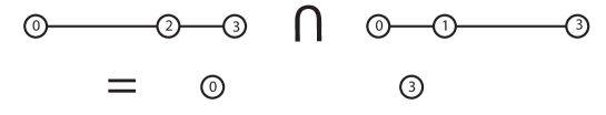
Figure 3. A codimension one toric fiber product that is not slow-varying.

5. Application: Markov bases for hierarchical models

Let $\Gamma$ be a simplicial complex with vertex set $V$, and let $d\in\mathbb{Z}^{V}_{\geq 2}$ a vector of integers. These data define a hierarchical model as in Section 1.1, and hence a toric ideal $I_{\Gamma,d}$. For any homogeneous ideal $I$, let $\mu(I)$ denote the largest degree of a minimal generator of $I$, which is an invariant of the ideal. This is a coarse measure of the complexity of the ideal $I$. If $\Gamma$ is a graph and $d_{v}=2$ for all $v\in V$, $\mu(I_{\Gamma,d})$, is an invariant of $\Gamma$ dubbed the Markov width in [5]. We calculate $\mu(\Gamma,d):=\mu(I_{\Gamma,d})$ for certain simplicial complexes $\Gamma$ and vectors $d$. The results of Section 4 are also useful to explicitly construct Markov bases of these hierarchical models.

The ideal $I_{\Gamma,d}$ is the toric ideal of a matrix $A_{\Gamma,d}$ with columns indexed by elements $i\in\mathrm{D}_{V}$. Each column is given by the formula

$$(A_{\Gamma,d})_{i}=\bigoplus_{F\in{\rm facet}(\Gamma)}e^{F}_{i_{F}}\in\bigoplus_{F\in{\rm facet}(\Gamma)}\mathbb{Z}^{\mathrm{D}_{F}}$$

where $\{e^{F}_{j_{F}}:j_{F}\in\mathrm{D}_{F}\}$ is the standard basis for $\mathbb{Z}^{\mathrm{D}_{F}}$. For $S\subset V$, let $\Gamma_{S}$ denote the induced subcomplex on $S$ (that is, $\Gamma_{S}=\{F\in\Gamma:F\subseteq S\}$). The matrix $A_{\Gamma_{S},d_{S}}$ induces a grading on $I_{\Gamma,d}$ by $\deg(p_{i})=(A_{\Gamma_{S},d_{S}})_{i_{S}}$. This grading is the $S$-grading.

Proposition 5.1.

Let $\Gamma$ be a simplicial complex with $\Gamma=\Gamma_{1}\cup\Gamma_{2}$, where the vertex set of $\Gamma_{1}$ and $\Gamma_{2}$ are $V_{1}$ and $V_{2}$, respectively. Let $S=V_{1}\cap V_{2}$ and suppose that $\Gamma_{1}\cap\Gamma_{2}=(\Gamma_{1})_{S}=(\Gamma_{2})_{S}$. Then

$$I_{\Gamma,d}=I_{\Gamma_{1},d_{V_{1}}}\times_{A_{\Gamma_{S},d_{S}}}I_{\Gamma_{2},d_{V_{2}}}.$$

Proof.

Since all the ideals are toric, it suffices to show that the fiber product of the vector configurations $A_{\Gamma_{1},d_{V_{1}}},A_{\Gamma_{2},d_{V_{2}}}$ equals $A_{\Gamma,d}$. For $i\in\mathrm{D}_{V}$ let $\mathbf{b}_{i_{V_{1}}}$ be the column of $A_{\Gamma_{1},d_{V_{1}}}$ indexed by $i_{V_{1}}$. Similarly, define $\mathbf{c}_{i_{V_{2}}}$, and $\mathbf{a}_{i_{S}}$ as the appropriate columns of $A_{\Gamma_{2},d_{V_{2}}}$ and $A_{\Gamma_{S},d_{S}}$, respectively. For $l=1,2$, let $\pi_{l}:\mathbb{R}^{\mathrm{D}_{V_{l}}}\rightarrow\mathbb{R}^{\mathrm{D}_{S}}$ be the linear projections induced by the grading that gives $\deg p_{i_{V_{1}}}=\deg p_{i_{V_{2}}}=\mathbf{a}_{i_{S}}$. The toric fiber product of vector configurations is

$$A_{\Gamma_{1},d_{V_{1}}}\times_{A_{\Gamma_{S},d_{S}}}A_{\Gamma_{2},d_{V_{2}}}=\{(\mathbf{b}_{j},\mathbf{c}_{k}:j\in d_{V_{1}},k\in d_{V_{2}},j_{S}=k_{S}\}.$$

This means that columns of the toric fiber product vector configuration have the form

$$\bigg{(}\bigoplus_{F\in{\rm facet}(\Gamma_{1})}\,\,e^{F}_{i_{F}}\bigg{)}\oplus\bigg{(}\bigoplus_{F\in{\rm facet}(\Gamma_{2})}\,\,e^{F}_{i_{F}}\bigg{)}.$$

If a facet $F$ appears in both $\Gamma_{1}$ and $\Gamma_{2}$, we can delete one of the corresponding collections of rows of $A_{\Gamma_{1},d_{V_{1}}}\times_{A_{\Gamma_{S},d_{S}}}A_{\Gamma_{2},d_{V_{2}}}$, without changing the kernel of the matrix, and hence the toric ideal. After eliminating repeats, we precisely have the matrix of $A_{\Gamma,d}$. ∎

In [16], the codimension of a hierarchical model ($\Gamma$,$d$) is given by the formula

(4) $$\sum_{F\notin\Gamma}\prod_{i\in F}(d_{i}-1).$$

Hence, the toric fiber product from Proposition 5.1 is a codimension zero toric fiber product if and only if $\Gamma_{S}=2^{S}$, and is a codimension one toric fiber product if and only if $\Gamma_{S}=2^{S}\setminus\{S\}$ and $d_{s}=2$ for all $s\in S$.

Proposition 5.2.

Let $\Gamma$ be a simplicial complex with $\Gamma=\Gamma_{1}\cup\Gamma_{2}$, where the vertex set of $\Gamma_{1}$ and $\Gamma_{2}$ are $V_{1}$ and $V_{2}$, respectively, and $\Gamma_{1}\cap\Gamma_{2}=(\Gamma_{1})_{S}=(\Gamma_{2})_{S}$. Let $\tilde{\Gamma}=\Gamma\cup 2^{[S]}$, and similarly $\tilde{\Gamma}_{1}=\Gamma_{1}\cup 2^{[S]}$ and $\tilde{\Gamma}_{2}=\Gamma_{2}\cup 2^{[S]}$. Then

$$\tilde{I}_{\Gamma,d}=I_{\tilde{\Gamma},d}=I_{\tilde{\Gamma}_{1},d_{V_{1}}}\times_{A_{2^{[S]},d_{S}}}I_{\tilde{\Gamma}_{2},d_{V_{2}}}.$$

Proof.

It suffices to show that for $I_{\Gamma,d}$, the construction of $\tilde{I}_{\Gamma,d}$ gives $I_{\tilde{\Gamma},d}$. Since $I_{\Gamma,d}$ is the kernel of a ring homomorphism, the construction of

$$\tilde{I}_{\Gamma,d}=(I_{\gamma,d}(P)+\langle p_{i}-P_{i}q_{i_{S}}:i\in d\rangle)\cap\mathbb{K}[p]$$

simply modifies that parametrization by taking $\tilde{\phi}(p_{i})=\phi(p_{i})q_{i_{S}}$. Thus, we have that $\tilde{I}_{\Gamma,d}=\ker\tilde{\phi}$ where

$$\tilde{\phi}(p_{i})=q_{i_{S}}\prod_{F\in{\rm facet}(\Gamma)}a^{F}_{i_{F}}.$$

We can delete all the $a^{F}_{i_{F}}$ parameters when $F\subseteq S$, since this does not change the kernel of the homomorphism. But then, this is precisely the parameterization associated with $\tilde{\Gamma}$. ∎

5.1. Small examples

In this section we restrict to the binary case where $d_{v}=2$ for all $v\in V$. To this end, let $\bf 2$ be the vector whose every coordinate is a $2$. We illustrate the constructions Quad, Lift, and Glue for small hierarchical models. Tableaux for binomials in hierarchical models have one column for each $i\in V$ (and as always one row per variable appearing in a monomial). For example, we represent the binomial $p_{111}p_{122}p_{212}p_{221}-p_{112}p_{121}p_{211}p_{222}$ as the tableau:

$$\begin{bmatrix}1&1&1\\ 1&2&2\\ 2&1&2\\ 2&2&1\end{bmatrix}-\begin{bmatrix}1&1&2\\ 1&2&1\\ 2&1&1\\ 2&2&2\end{bmatrix}.$$

Lemma 5.3.

1. Let $S_{V}=2^{V}\setminus\{V\}$, be the boundary of a $(\#V-1)$-dimensional simplex. Then $I_{S_{V},{\bf 2}}$ is generated by a single binomial:

   $$\prod_{i\in\mathrm{D}_{V}:\|i\|_{1}{\rm even}}p_{i}-\prod_{i\in\mathrm{D}_{V}:\|i\|_{1}{\rm odd}}p_{i}.$$

2. Let $\Gamma$ be a simplicial complex on $V$, let

   $${\rm cone}_{v}(\Gamma)=\Gamma\cup\{F\cup\{v\}:F\in\Gamma\}$$

   be the cone over $\Gamma$ with apex $v$, and let $\mathcal{F}$ be a (minimal) generating set of $I_{\Gamma,d}$. Then $I_{{\rm cone}_{v}(\Gamma),d_{V\cup\{v\}}}$ is (minimally) generated by

   $${\rm cone}_{v}(\mathcal{F})=\left\{p_{i_{1},j}\cdots p_{i_{n},j}-p_{i_{1}^{\prime},j}\cdots p_{i_{n}^{\prime},j}:p_{i_{1}}\cdots p_{i_{n}}-p_{i_{1}^{\prime}}\cdots p_{i_{n}^{\prime}}\in\mathcal{F}\mbox{ and }j\in[d_{v}]\right\}.$$

Proof.

   
(1) According to the dimension formula (4), $I_{S_{V},{\bf 2}}$ is generated by a single equation. The proof of (4) in [16] shows that the given binomial generates the ideal.

(2) This follows because one can rearrange the rows and columns of $A_{{\rm cone}_{v}(\Gamma),d_{V\cup\{v\}}}$ so that it is a block diagonal matrix with $d_{v}$ diagonal blocks with the matrix $A_{\Gamma,d}$ along the diagonal. This decomposition appears in [17]. ∎

Example 5.4 (Binary four-cycle).

Let $C$ be a four-cycle with edges $12,13,24,34$. The cycle decomposes as the union of two paths with edges $12,13$ and $24,34$. With $V_{1}=\{1,2,3\}$ and $V_{2}=\{2,3,4\}$, $I_{C,{\bf 2}}$ is the toric fiber product of $I_{C_{V_{1}},{\bf 2}}$ and $I_{C_{V_{2}},{\bf 2}}$. According to Lemma 5.3, the Markov basis of a path of length three with edges $12,13$, consists of the two elements

$$\begin{bmatrix}i&1&1\\ i&2&2\\ \end{bmatrix}-\begin{bmatrix}i&1&2\\ i&2&1\\ \end{bmatrix},\quad\quad i\in\{1,2\}.$$

Similarly, the Markov basis for the path with edges $24,34$ consists of the two elements

$$\begin{bmatrix}1&1&l\\ 2&2&l\\ \end{bmatrix}-\begin{bmatrix}1&2&l\\ 2&1&l\\ \end{bmatrix},\quad\quad l\in\{1,2\}.$$

These Markov bases are slow-varying with respect to the codimension one toric fiber product obtained by the overlap complex, which is two isolated vertices $2,3$. The vector $\mathbf{h}$ for the complex of two isolated vertices is

$$\begin{bmatrix}1&1\\ 2&2\\ \end{bmatrix}-\begin{bmatrix}1&2\\ 2&1\\ \end{bmatrix}.$$

The glue operation on these Markov bases produces four moves:

$$\begin{bmatrix}i&1&1&l\\ i&2&2&l\\ \end{bmatrix}-\begin{bmatrix}i&1&2&l\\ i&2&1&l\\ \end{bmatrix},\quad\quad i,l\in\{1,2\}.$$

The associated codimension zero toric fiber product is the hierarchical model associated to the complex $\Gamma=C\cup\{\{2,3\}\}$, two triangles glued along an edge. It produces four quadratic elements of ${\rm Quad}:$

$$\begin{bmatrix}1&j&k&1\\ 2&j&k&2\\ \end{bmatrix}-\begin{bmatrix}1&j&k&2\\ 2&j&k&1\\ \end{bmatrix},\quad\quad j,k\in\{1,2\}.$$

A triangle with edges $12,13,23$ has a single quartic move in its Markov basis, which is:

$$\begin{bmatrix}1&1&1\\ 1&2&2\\ 2&1&2\\ 2&2&1\end{bmatrix}-\begin{bmatrix}1&1&2\\ 1&2&1\\ 2&1&1\\ 2&2&2\end{bmatrix}.$$

Lifting this move produces $16$ quartic Markov basis elements:

$$\begin{bmatrix}1&1&1&l_{1}\\ 1&2&2&l_{2}\\ 2&1&2&l_{3}\\ 2&2&1&l_{4}\end{bmatrix}-\begin{bmatrix}1&1&2&l_{3}\\ 1&2&1&l_{4}\\ 2&1&1&l_{1}\\ 2&2&2&l_{2}\end{bmatrix}\quad\quad l_{1},l_{2},l_{3},l_{4}\in\{1,2\}.$$

Similarly, the lifting operation from the cycle with edges $23,24,34$ produces

$$\begin{bmatrix}i_{1}&1&1&1\\ i_{2}&1&2&2\\ i_{3}&2&1&2\\ i_{4}&2&2&1\end{bmatrix}-\begin{bmatrix}i_{1}&1&1&2\\ i_{2}&1&2&1\\ i_{3}&2&1&1\\ i_{4}&2&2&2\end{bmatrix}\quad\quad i_{1},i_{2},i_{3},i_{4}\in\{1,2\}.$$

Theorem 4.12 implies that the lifts of $8$ quadrics and $32$ quartics generate the $I_{C,{\bf 2}}$. However, these elements do not form a minimal generating set. Direct computation in 4ti2 [1] shows that a minimal Markov basis contains all 8 quadrics but only 8 of the quartics.

Similar arguments and the description of Markov bases of small cycles in Lemma 5.9 can be used to get an explicit description of Markov bases of the four-cycles that appear in Example 1.2. We can also produce analogous results for higher dimensional complexes.

Theorem 5.5.

Let $B_{n}$ be the simplicial complex with vertex set $[n+2]$ and minimal non-faces $[n]$ and $\{n+1,n+2\}$. The ideal $I_{B_{n},{\bf 2}}$ has a generating set consisting of binomials of degrees $2,2^{n-1},$ and $2^{n}$.

Proof.

For $i=1,2$ let $\Gamma_{i}$ be the cone $B_{n}\setminus(n+i)$ over the boundary of the simplex on $[n]$. Then $B_{n}=\Gamma_{1}\cup\Gamma_{2}$. According to part (1) of Lemma 5.3 the Markov basis of $I_{\Gamma_{1}\cap\Gamma_{2},{\bf 2}}$ consists of a single element of degree $2^{n-1}$; and according to part (2) the ideals $I_{\Gamma_{i},{\bf 2}}$ are each generated by two binomials of degree $2^{n-1}$. Since $2^{n-1}<2\times 2^{n-1}$, by Proposition 4.11, the Markov bases for $I_{\Gamma_{1},{\bf 2}}$ and $I_{\Gamma_{2},{\bf 2}}$ are slow-varying with respect to the Markov basis of $I_{\Gamma_{1}\cap\Gamma_{2},{\bf 2}}$. The set of glue moves consists of $4$ binomials of degree $2^{n-1}$.

The simplicial complex $\tilde{\Gamma}$ appearing in the associated codimension zero toric fiber product has $[n]$ as an additional face. Consequently it consists of the boundaries of two $(n-1)$-dimensional simplices that share a single facet. By part (1) of Lemma 5.3, the Markov basis of the boundary of an $(n-1)$-dimensional simplex consists of a single element of degree $2^{n}$. The lifting operation preserves degree and produces $2^{2^{n}}$ elements per boundary simplex, for a total of $2^{2^{n}+1}$ elements of degree $2^{n}$. Finally, there are $2^{n}$ quadrics in ${\rm Quad}$. Theorem 4.12 shows that the union of all these elements is a Markov basis. ∎

The simplicial complex $B_{n}$ is the boundary of the polytope that is a bipyramid over a simplex. In particular, it is a simplicial sphere. Theorem 5.5 and the results of [28] provide evidence for the following conjecture.

Conjecture 5.6.

Let $\Gamma$ be a triangulation of a sphere of dimension $n$. Then the Markov basis of $I_{\Gamma,{\bf 2}}$ consists of elements of degree at most $2^{n+1}$.

To conclude this section, we give an example which shows how the gluing operation can produce Markov basis elements of larger degree than either of the constituent binomials.

Example 5.7.

Let $G$ be the graph with vertex set $[5]$ and all edges except $1$–$5$, and assume that $d={\bf 2}$. Thus, $G$ consists of two $K_{4}$ graphs glued along an empty triangle. The Markov basis for $K_{4}$ consists of $20$ elements of degree four and $40$ elements of degree six. The overlap triangle is the boundary of a simplex, whose Markov basis consists of a single element of degree four. Since $6<2\times 4$, by Proposition 4.11 the Markov bases of each of the $K_{4}$ are slow-varying. Consider the following two binomials in the ideal of $K_{4}$:

$$\begin{bmatrix}1&1&1&1\\ 2&1&2&2\\ 2&2&1&2\\ 2&2&2&1\\ \hline\cr 1&1&1&1\\ 1&2&2&2\\ \end{bmatrix}-\begin{bmatrix}1&1&1&2\\ 1&1&2&1\\ 1&2&1&1\\ 2&2&2&2\\ \hline\cr 2&1&1&1\\ 2&2&2&2\end{bmatrix},\quad\quad\begin{bmatrix}1&1&1&1\\ 1&2&2&1\\ 2&1&2&1\\ 2&2&1&2\\ \hline\cr 1&1&2&2\\ 2&2&1&2\\ \end{bmatrix}-\begin{bmatrix}1&1&2&1\\ 1&2&1&2\\ 2&1&1&2\\ 2&2&2&2\\ \hline\cr 1&1&2&1\\ 2&2&1&1\end{bmatrix}.$$

The first sextic comes from the $K_{4}$ on vertex set $\{1,2,3,4\}$ and the second one from the $K_{4}$ on vertex set $\{2,3,4,5\}$. In the columns corresponding to $\{2,3,4\}$ they agree in the first four rows and disagree in the last two rows. This means that upon gluing these sextics, we produce moves of degree $4+2+2=8$. In particular we get

$$\begin{bmatrix}1&1&1&1&1\\ 2&1&2&2&1\\ 2&2&1&2&1\\ 2&2&2&1&2\\ \hline\cr 1&1&1&1&m_{1}\\ 1&2&2&2&m_{2}\\ \hline\cr i_{1}&1&1&2&2\\ i_{2}&2&2&1&2\end{bmatrix}-\begin{bmatrix}1&1&1&2&1\\ 1&1&2&1&2\\ 1&2&1&1&2\\ 2&2&2&2&2\\ \hline\cr 2&1&1&1&m_{1}\\ 2&2&2&2&m_{2}\\ \hline\cr i_{1}&1&1&2&1\\ i_{2}&2&2&1&1\end{bmatrix},\quad\quad i_{1},i_{2},m_{1},m_{2}\in\{1,2\}.$$

In this example gluing yields degrees four, six, and eight. Lifting produces Markov basis elements of degrees four and six. Direct computation with 4ti2 shows, however, that a minimal Markov basis of this model contains only binomials of degree two, four, and six. Therefore the gluing operation may produce elements of unnecessarily large degree.

5.2. Cycles and ring graphs

In this subsection, and the next, $\Gamma=G$ is a graph. We start with cycles and graphs that can be easily constructed from cycles, then explore $K_{4}$-minor free graphs, providing a new proof of the main result in [21]. To set up induction we provide the Markov bases of simple graphs.

Lemma 5.8.

Let $P$ be a path and $d\in\mathbb{Z}^{V}_{\geq 2}$ arbitrary, then $\mu(P,d)=2$.

Proof.

This follows from Theorem 4.3 or the results on decomposable simplicial complexes in [8, 37]. ∎

Lemma 5.9 (Small Graphs).

1. Let $K_{3}$ be the triangle. The following table contains known values of $\mu(K_{3},d)$:

   $$\begin{array}[]{c|cccccc}d_{1}&2&3&3&3&3&4\\ d_{2}&p&3&3&3&4&4\\ d_{3}&q&3&4&q\geq 5&4&4\\ \hline\cr\mu(I_{K_{3},d})&\min(2p,2q)&6&8&10&12&14\\ \end{array}$$

2. If $C$ is a four-cycle with edges $12,23,34,41$, then $\mu(C,d)$ takes the following values

   $$\begin{array}[]{c|cccccccc}d_{1}&2&2&2&2&2&2&2&3\\ d_{2}&2&2&2&2&2&2&3&3\\ d_{3}&3&3&3&4&4&5&3&3\\ d_{4}&3&4&5&4&5&5&3&3\\ \hline\cr\mu(C,d)&6&6&6&8&8&10&6&6\\ \end{array}$$

3. If $C$ is a five-cycle with edges $12,23,34,45,51$, $d_{1}=d_{2}=2$, and $d_{3}=d_{4}=d_{5}=3$, then $\mu(C,d)=6$.

4. Let $K_{2,3}$ be the complete bipartite graph on $\{1,2\}$ and $\{3,4,5\}$. If $d_{1}=d_{2}=3$ and $d_{3}=d_{4}=d_{5}=2$, then $\mu(K_{2,3},d)=6$.

5. The complete graph $K_{4}$ with $d={\bf 2}$ satisfies $\mu(K_{4},{\mathbf{2}})=6$.

Proof.

The computation for $K_{3}$ with $d=(2,p,q)$ is contained in the original work of Diaconis and Sturmfels [6]. The values for $d=(3,3,q)$ were determined by Aoki and Takemura [2]. All other values have been computed using 4ti2 and Markov bases are available on the Markov Basis Database [19]. ∎

Lemma 5.10.

Let $G$ be a graph, and $V_{1},V_{2}\subseteq V$ such that $V_{1}\cup V_{2}=V$, $G=G_{V_{1}}\cup G_{V_{2}}$ and either $V_{1}\cap V_{2}=\{u\}$ or $V_{1}\cap V_{2}=\{u,v\}$ with $uv$ an edge of $G$. Then

$$\mu(G,d)=\max(2,\mu(G_{V_{1}},d_{V_{1}}),\mu(G_{V_{2}},d_{V_{2}})).$$

Proof.

In either case $I_{G,d}$ is a codimension zero toric fiber product and Theorem 4.3 applies. The statement also follows from results on reducible hierarchical model in [9, 16, 34]. ∎

Lemma 5.11.

Let $G$ be a graph, and $V_{1},V_{2}\subseteq V$ such that $V_{1}\cup V_{2}=V$, $G=G_{V_{1}}\cup G_{V_{2}}$ and $V_{1}\cap V_{2}=\{u,v\}$ where $uv$ is not an edge of $G$, and suppose that $d_{u}=d_{v}=2$. Further suppose that $\mu(G_{V_{1}},d_{V_{1}})=\mu(G_{V_{2}},d_{V_{2}})=2$. Then

$$\mu(G,d)\leq\max(2,\mu(G_{V_{1}}\cup\,uv,d_{V_{1}}),\mu(G_{V_{2}}\cup\,uv,d_{V_{2}})).$$

Proof.

The intersection of $G_{V_{1}}$ and $G_{V_{2}}$ is the graph with two nodes, and no edges. Since $d_{u}=d_{v}=2$, the dimension formula (4) implies that this is a codimension one toric fiber product. The toric ideal of the graph consisting of two isolated nodes, and $d_{u}=d_{v}=2$ is generated by a single quadratic binomial, by Lemma 5.3. Furthermore, the fact that $\mu(G_{V_{1}},d_{V_{1}})=\mu(G_{V_{2}},d_{V_{2}})=2$, and that hierarchical models have no Markov basis elements of degree one, implies that the Markov bases of $I_{G_{V_{1}},d_{V_{1}}}$ and $I_{G_{V_{2}},d_{V_{2}}}$ are slow-varying, by Proposition 4.11. Hence Theorem 4.12 shows that the Markov basis of $I_{G,d}$ consists of the glued elements of the Markov bases of $I_{G_{V_{1}},d_{V_{1}}}$ and $I_{G_{V_{2}},d_{V_{2}}}$, together with the Markov basis of the associated codimension zero toric fiber product, which is

$$I_{G\cup\,uv,d}=I_{G_{V_{1}}\cup\,uv,d_{V_{1}}}\times_{\mathcal{A}}I_{G_{V_{2}}\cup\,uv,d_{V_{2}}},$$

by Proposition 5.2. Since we only ever glue quadrics along a quadric, the resulting binomial is also of degree two. The generators of the associated codimension zero toric fiber product consists of quadratic elements and lifts of generators of $I_{G_{V_{1}}\cup\,uv,d_{V_{1}}}$ and $I_{G_{V_{2}}\cup\,uv,d_{V_{2}}}$. Since lifting preserves degrees, the quantity $\max(2,\mu(G_{V_{1}}\cup\,uv,d_{V_{1}}),\mu(G_{V_{2}}\cup\,uv,d_{V_{2}}))$ is the maximum degree of a generator of the associated codimension zero toric fiber product. ∎

Lemma 5.12.

Let $C$ be a cycle with vertex set $V$ and $d\in\mathbb{Z}^{V}_{\geq 2}$.

• If $C$ contains no edge $uv$ with $d_{u},d_{v}>2$ then $\mu(C,d)=4$.

• If all $d_{v}\leq 3$ and $C$ contains no path $u_{1}u_{2}u_{3}u_{4}$ with all $d_{u_{i}}>2$, then $\mu(C,d)\leq 6$.

• If all $d_{v}\leq 4$ and $C$ contains no path $u_{1}u_{2}u_{3}$ with all $d_{u_{i}}>2$, then $\mu(C,d)\leq 8$.

• If all $d_{v}\leq 5$ and $C$ contains no path $u_{1}u_{2}u_{3}$ with all $d_{u_{i}}>2$, then $\mu(C,d)\leq 10$.

Proof.

We give a detailed proof of (1). According to Lemma 5.9 the statement holds for cycles of length three. We proceed by induction on the length of $C$. There are always two non-adjacent vertices $u$ and $v$ in $C$ with $d_{u}=d_{v}=2$. Let $V_{1}$ be the set of vertices on one of the paths in $C$ from $u$ to $v$, and let $V_{2}$ be the set of vertices on the other path. According to Lemma 5.8 the Markov width of paths is two. By induction we find $\mu(G_{V_{1}}\cup\,uv,d_{V_{1}})=4$ and $\mu(G_{V_{2}}\cup\,uv,d_{V_{2}})=4$, since those graphs are shorter cycles than $C$ satisfying the conditions in (1). By Lemma 5.11, the Markov width of $\mu(C,d)=4$. Statements (2)-(4) follow by the same inductive argument and reducing to the small graphs in Lemma 5.9. ∎

Cycles can be patched together to form larger graph classes, for example ring graphs.

Definition 5.13.

A ring graph is a graph that can be recursively constructed from paths and cycles by disjoint unions, identifying a vertex of disjoint components, and identifying edges on disjoint components. An outerplanar graph is a graph with a planar embedding such that all vertices are on a circle.

Outerplanar graphs are also characterized as the largest minor closed class that excludes $K_{4}$ and $K_{2,3}$. This in particular implies that all outerplanar graphs are series-parallel since they have no $K_{4}$-minors. It is easy to see that outerplanar graphs are ring graphs. Recall that a graph is $k$-connected if there is no way to disconnect it by removing at most $k-1$ vertices. We need to describe how to decompose 2-connected ring graphs into cycles.

Definition 5.14.

A cycle decomposition of a 2-connected ring graph $G$ is a sequence $C_{1},C_{2},\ldots,C_{k}$ of cycles in $G$ such that

• the union of all $C_{i}$ is $G,$ and

• the intersection of $C_{1}\cup\cdots\cup C_{i}$ and $C_{i+1}$ is an edge for $1\leq i<k$.

Any $2$-connected ring graph must have a cycle decomposition, since a $2$-connected ring graph is obtained by only identifying edges in disjoint components.

Theorem 5.15.

Let $G$ be a ring graph whose maximal 2-connected subgraphs are $G_{1},G_{2},\ldots,G_{l}$ and assume that $C_{1}^{i},C_{2}^{i},\ldots,C_{k_{i}}^{i}$ is a cycle decomposition of $G_{i}$ for all $1\leq i\leq l$. If for all $C=C^{i}_{j},$

• there is no edge $uv$ in $C$ with $d_{u},d_{v}>2$ then $\mu(G,d)\leq 4$.

• all $d_{v}\leq 3$ and there is no path $u_{1}u_{2}u_{3}u_{4}$ in $C$ with all $d_{u_{i}}>2$, then $\mu(G,d)\leq 6$.

• all $d_{v}\leq 4$ and there is no path $u_{1}u_{2}u_{3}$ in $C$ with all $d_{u_{i}}>2$, then $\mu(G,d)\leq 8$.

• all $d_{v}\leq 5$ and there is no path $u_{1}u_{2}u_{3}$ in $C$ with all $d_{u_{i}}>2$, then $\mu(G,d)\leq 10$.

Proof.

This follows directly from Lemma 5.8, Lemma 5.10, and Lemma 5.12. ∎

Definition 5.16.

A graph $G$ is Markov slim, if for every independent set $I$ of $G$ the model with $d_{v}\geq 2$ for $v\in I$ and $d_{v}=2$ for $v\in V(G)\setminus I$ has Markov width at most four.

Theorem 5.17.

The maximal minor-closed class of Markov slim graphs is the outerplanar graphs.

Proof.

By Theorem 5.15 the outerplanar graphs are Markov slim since they are ring graphs. Say that there is a minor closed class larger than the outerplanar graphs, in which every graph is Markov slim. Then this class either contains $K_{4}$ or $K_{2,3}$. By parts (4) and (5) of Lemma 5.9 neither $K_{4}$ nor $K_{2,3}$ are Markov slim. ∎

Repeated toric fiber products of cycles reduce computations of the Markov width to the three cycle. Therefore the following conjecture seems natural.

Conjecture 5.18.

Let $C$ be a cycle of length $n$, with edges $12,23,\ldots,n1$. Then the Markov width $\mu(C,d)$ equals

$$\max_{i=1,\ldots,n}\mu(K_{3},(d_{i},d_{i+1},d_{i+2}))$$

where the indices $i,i+1,i+2$ are considered cyclically modulo $n$.

Our results so far only work with codimension one toric fiber products, which do not raise the degree of generators in the cycle case, and hence we always glued paths at a pair of vertices $u,v$ where $d_{u}=d_{v}=2$. It is not clear whether or not this remains true for larger values of $d_{u},d_{v}$.

5.3. Binary series-parallel graphs

To prove Theorem 1.1 we apply a classical decomposition of $K_{4}$-minor free graphs.

Definition 5.19.

The class $SP$ of connected series-parallel graph is the smallest collection of graphs satisfying the following properties.

• Each graph $G\in SP$ has two distinguished vertices, the top and the bottom vertex, which are different.

• The graph $K_{2}$ is in $SP$.

• If $G_{1}$ and $G_{2}$ are in $SP$ with tops and bottoms $t_{1},t_{2}$, $b_{1},b_{2}$ respectively, then

  Series construction:

  the graph obtained from $G_{1}$ and $G_{2}$ by identifying $t_{1}$ and $b_{2}$ and calling $b_{1}$ and $t_{2}$ the new bottom and top also belongs to $SP$;

  Parallel construction:

  the graph obtained form $G_{1}$ and $G_{2}$ by identifying $t_{1}$ and $t_{2}$ and $b_{1}$ and $b_{2}$ (and calling these the new top and bottom) is also in $SP$.

In a graph without $K_{4}$-minors, every 2-connected component is a series-parallel graph (see [7, Chapter 7]). Since gluing two graphs at a vertex is a codimension zero toric fiber product, to prove Theorem 1.1, we can restrict to series-parallel graphs. One tool is the following lemma about choices that can be made in the parallel construction.

Lemma 5.20.

Suppose that $G\in SP$ has at least four vertices. Then $G$ can be obtained by series or parallel construction from two graphs $G_{1}$ and $G_{2}$ each with fewer vertices than $G$.

Proof.

The series construction of $G_{1}$ and $G_{2}$ clearly produces a graph $G$ with a larger number of vertices. For the parallel construction, if both $G_{1}$ and $G_{2}$ are not single edges then their parallel construction has more vertices than either $G_{1}$ or $G_{2}$. The only non-trivial case is when one of the two graphs, say $G_{1}$, is a single edge.

We can assume $G_{2}$ is neither a path of one or two edges, nor $K_{3}$, since then the resulting graph would have less than three vertices. The graph $G_{2}$ is obtained either by a series or by a parallel construction from two graphs $G_{3}$ and $G_{4}$. In the case of a parallel construction, consider new graphs $\tilde{G_{3}}$ and $\tilde{G_{4}}$ with an edge glued in from $t$ to $b$ in both cases. The resulting parallel construction of $\tilde{G_{3}}$ and $\tilde{G_{4}}$ gives the same graph as the parallel construction of $G_{1}$ and $G_{2}$. In the case of a series construction, one of the graphs $G_{3}$ or $G_{4}$ has $\geq 3$ vertices. Assume that graph is $G_{4}$. A series construction of $G_{1}$ with $G_{3}$ followed by a parallel construction of the result with $G_{4}$ gives the original graph. We may have to rearrange the tops and bottoms during this construction, but doing so does not change the property of being a series-parallel graph. ∎

Theorem 5.21.

If $G$ is a connected series-parallel graph with top $t$ and bottom $b$, then $\mu(G,{\bf 2})=4$ and a Markov basis of $I_{G,{\bf 2}}$ can be chosen to consist of:

• Degree four binomials whose terms have the same degree on the $bt$ subcomplex.

• Degree two binomials that are slow-varying on the $bt$ subcomplex.

Proof.

We proceed by induction on the number of vertices of the graph. The statement is trivially true for connected series-parallel graphs with one or two vertices, since they have empty Markov basis. There are two graphs with three vertices to consider. For the triangle $I_{K_{3},{\bf 2}}$ there is one degree four generator and it must project to the zero polynomial along the $bt$ edge, since that edge belongs to $K_{3}$. In the case of the path with three vertices, there are two quadratic generators, which are slow-varying by Proposition 4.11.

Now let $G$ be a series-parallel graph with at least four vertices. By Lemma 5.20 it can be built from two graphs $G_{1}$ and $G_{2}$ with strictly smaller numbers of vertices by either a series or a parallel construction. We must show that properties $(1)$ and $(2)$ of the Markov basis are preserved under either of these constructions.

First suppose that $G$ is obtained from $G_{1}$ and $G_{2}$ by a series construction. There are three types of generators that arise. The generators are given by:

Lift 1:

lifting generators from $I_{G_{1},{\bf 2}}$ while being constant on $G_{2}$;

Lift 2:

lifting generators from $I_{G_{2},{\bf 2}}$ while being constant on $G_{1}$;

Quad:

quadratic moves.

Since Lifting preserves degrees we obtain only moves of degree two and four. Quadratic moves are slow-varying by Proposition 4.11, thus we must show that the degree four moves can be chosen so that their projections on the $bt$ edge are constant. The crucial idea is that the degree four generators all come from three-cycles, since we are always only using series or parallel construction. The quartic generator for $I_{K_{3},{\bf 2}}$ is

$$\begin{bmatrix}1&1&1\\ 1&2&2\\ 2&1&2\\ 2&2&1\end{bmatrix}-\begin{bmatrix}1&1&2\\ 1&2&1\\ 2&1&1\\ 2&2&2\end{bmatrix}.$$

Any subsequent appearance of a quartic is a lift of this move in some way and must be obtained by using a single edge or vertex in $K_{3}$ and performing a sequence of lifts. The pair $bt$ cannot go from an added vertex to the third vertex of the underlying $K_{3}$, otherwise we would be able to construct graphs that have $K_{4}$ as a minor. Thus, $b$ and $t$ belong to the gluing edge, or a subset of the lifted vertices. However, by construction of the lift operation, the binomial projects to zero when restricted to such a subset of vertices.

If $G$ is obtained from a parallel construction of $G_{1}$ and $G_{2}$, then the top and bottom vertices can be adjacent or not. If they are adjacent, then we are gluing along an edge. All generators of $I_{G_{1},{\bf 2}}$ and $I_{G_{2},{\bf 2}}$ project to zero along this edge by properties of the lift operation. If the special vertices are not adjacent, we have a codimension one toric fiber product. The associated codimension zero product consists of series-parallel graphs with fewer vertices. By the argument in the preceding paragraphs, all Markov basis elements obtained from the associated codimension zero toric fiber product satisfies either (1) or (2). Finally, consider ${\operatorname{\mathbf{Glue}}}(\mathcal{F},\mathcal{G})$. Since all Markov bases satisfy (1) and (2), we only ever glue quadrics, producing more quadrics, which are slow-varying by Proposition 4.11. ∎

Instead of using binary variables for the triangle in the proof, one could have used larger values of $d_{v}$ on the vertex of the triangle that is never involved in gluing or identification. This would have given an alternative but less descriptive proof of Theorem 5.15. The procedure yields a larger class than ring graphs, but it is not true that larger $d_{v}$ on independent sets always produce Markov width four, as illustrated earlier by the fact that $K_{2,3}$ is not Markov slim.

There are further applications of higher codimension toric fiber products in algebraic statistics lurking. For example, ideals of graph homomorphisms [12] generalize classes of toric ideals in algebraic statistics. Given graphs $G$ and $H$, potentially with loops, the ideal of graph homomorphisms from $G$ to $H$ is $I_{G\rightarrow H}$. In this language, binary hierarchical models arise as the special case where $H=K_{2}^{o}$ is the complete graph with loops. If $H$ is an edge with one loop, then the homomorphisms from $G$ to $H$ correspond to the independent sets of $G$. It is known that $I_{G\rightarrow H}$ is quadratically generated if $G$ is bipartite, or becomes bipartite after the removal of one vertex [12]. Using Theorem 5.21 as a template, one derives that $I_{G\rightarrow H}$ is quadratically generated for series-parallel $G$.

Some toric ideals are not toric fiber products themselves, but project to one. With control over the projection one may be able to find a Markov basis anyway. An Example is Norén’s proof of a conjecture by Haws, Martin del Campo, Takemura, and Yoshida [26].

6. Application: conditional independence ideals

A basic problem in the algebraic study of conditional independence is to understand primary decompositions of CI-ideals. For instance, if a conditional independence model comes from a graph, the minimal primes provide information about families of probability distributions that satisfy the conditional independence constraints but do not factorize according to the graph. Moreover, primary decompositions can provide information about the connectivity of random walks using Markov subbases [20].

In this section $J$ is the generic letter denoting an ideal. This is to avoid confusion between the ideals $I_{G}$ of Section 5 and the CI-ideals $J_{G}$ in Section 6.2. The results in this section are independent of $d=(d_{v})_{v\in V}$, the vector of cardinalities. It is fixed arbitrarily and does not appear in the notation.

Assume $\mathcal{M}$ is a conditional independence model and $J_{\mathcal{M}}$ its CI-ideal. Our goal is to describe conditions under which there exist suitable conditional independence models $\mathcal{M}_{1}$ and $\mathcal{M}_{2}$ such that

$$J_{\mathcal{M}}=J_{\mathcal{M}_{1}}\times_{\mathcal{A}}J_{\mathcal{M}_{2}}.$$

When $J_{\mathcal{M}}$ is as a toric fiber product, the results of Section 3 yield a primary decomposition of $J_{\mathcal{M}}$ from primary decompositions of $J_{\mathcal{M}_{1}}$ and $J_{\mathcal{M}_{2}}$, greatly reducing the necessary computational efforts. This seems to work best in the case of codimension zero toric fiber products. At this moment it is not clear if there is a use for higher codimension toric fiber products in analyzing conditional independence models.

We first develop a general theory for arbitrary conditional independence models. Then we apply it to global Markov ideals of graphs, showing that they are toric fiber products if the graph has a decomposition along a clique.

We assume the same setup as in Section 1.1 for hierarchical models. Let $A,B,C$ be three pairwise disjoint subsets of $V$, and $D\mathrel{\mathop{:}}=V\setminus(A\cup B\cup C)$. If $D\neq\emptyset$, then $p_{i_{A}i_{B}i_{C}+}\mathrel{\mathop{:}}=\sum_{i_{D}\in\mathrm{D}_{D}}p_{i_{A}i_{B}i_{C}i_{D}}$. The conditional independence (CI) ideal $J_{\left.A\mathchoice{\mathrel{\hbox to0.0pt{$\displaystyle\perp$\hss}\mkern 2.0mu{\displaystyle\perp}}}{\mathrel{\hbox to0.0pt{$\textstyle\perp$\hss}\mkern 2.0mu{\textstyle\perp}}}{\mathrel{\hbox to0.0pt{$\scriptstyle\perp$\hss}\mkern 2.0mu{\scriptstyle\perp}}}{\mathrel{\hbox to0.0pt{$\scriptscriptstyle\perp$\hss}\mkern 2.0mu{\scriptscriptstyle\perp}}}B\,\middle|C\right.{}}$ is

$$J_{\left.A\mathchoice{\mathrel{\hbox to0.0pt{$\displaystyle\perp$\hss}\mkern 2.0mu{\displaystyle\perp}}}{\mathrel{\hbox to0.0pt{$\textstyle\perp$\hss}\mkern 2.0mu{\textstyle\perp}}}{\mathrel{\hbox to0.0pt{$\scriptstyle\perp$\hss}\mkern 2.0mu{\scriptstyle\perp}}}{\mathrel{\hbox to0.0pt{$\scriptscriptstyle\perp$\hss}\mkern 2.0mu{\scriptscriptstyle\perp}}}B\,\middle|C\right.{}}\mathrel{\mathop{:}}=\left\langle p_{i_{A}i_{B}i_{C}+}p_{j_{A}j_{B}i_{C}+}-p_{i_{A}j_{B}i_{C}+}p_{j_{A}i_{B}i_{C}+}:i_{A},j_{A}\in\mathrm{D}_{A},i_{B},j_{B}\in\mathrm{D}_{B},i_{C}\in\mathrm{D}_{C}\right\rangle.$$

An argument similar to that in Section 1.2 shows that this ideal is prime. For a collection

$$\mathcal{M}=\{\left.A_{1}\mathchoice{\mathrel{\hbox to0.0pt{$\displaystyle\perp$\hss}\mkern 2.0mu{\displaystyle\perp}}}{\mathrel{\hbox to0.0pt{$\textstyle\perp$\hss}\mkern 2.0mu{\textstyle\perp}}}{\mathrel{\hbox to0.0pt{$\scriptstyle\perp$\hss}\mkern 2.0mu{\scriptstyle\perp}}}{\mathrel{\hbox to0.0pt{$\scriptscriptstyle\perp$\hss}\mkern 2.0mu{\scriptscriptstyle\perp}}}B_{1}\,\middle|C_{1}\right.{},\ldots,\left.A_{r}\mathchoice{\mathrel{\hbox to0.0pt{$\displaystyle\perp$\hss}\mkern 2.0mu{\displaystyle\perp}}}{\mathrel{\hbox to0.0pt{$\textstyle\perp$\hss}\mkern 2.0mu{\textstyle\perp}}}{\mathrel{\hbox to0.0pt{$\scriptstyle\perp$\hss}\mkern 2.0mu{\scriptstyle\perp}}}{\mathrel{\hbox to0.0pt{$\scriptscriptstyle\perp$\hss}\mkern 2.0mu{\scriptscriptstyle\perp}}}B_{r}\,\middle|C_{r}\right.{}\}$$

of CI-statements, the CI-ideal is the sum of the ideals of its statements:

$$J_{\mathcal{M}}=J_{\left.A_{1}\mathchoice{\mathrel{\hbox to0.0pt{$\displaystyle\perp$\hss}\mkern 2.0mu{\displaystyle\perp}}}{\mathrel{\hbox to0.0pt{$\textstyle\perp$\hss}\mkern 2.0mu{\textstyle\perp}}}{\mathrel{\hbox to0.0pt{$\scriptstyle\perp$\hss}\mkern 2.0mu{\scriptstyle\perp}}}{\mathrel{\hbox to0.0pt{$\scriptscriptstyle\perp$\hss}\mkern 2.0mu{\scriptscriptstyle\perp}}}B_{1}\,\middle|C_{1}\right.{}}+\cdots+J_{\left.A_{r}\mathchoice{\mathrel{\hbox to0.0pt{$\displaystyle\perp$\hss}\mkern 2.0mu{\displaystyle\perp}}}{\mathrel{\hbox to0.0pt{$\textstyle\perp$\hss}\mkern 2.0mu{\textstyle\perp}}}{\mathrel{\hbox to0.0pt{$\scriptstyle\perp$\hss}\mkern 2.0mu{\scriptstyle\perp}}}{\mathrel{\hbox to0.0pt{$\scriptscriptstyle\perp$\hss}\mkern 2.0mu{\scriptscriptstyle\perp}}}B_{r}\,\middle|C_{r}\right.{}}.$$

In statistics one is usually not interested in all of the variety of a CI-ideal, but only its intersection with the set of probability distributions. The following properties of CI-ideals imply well-known properties of conditional independence.

Proposition 6.1.

The following ideal containments hold:

• $J_{\left.A\mathchoice{\mathrel{\hbox to0.0pt{$\displaystyle\perp$\hss}\mkern 2.0mu{\displaystyle\perp}}}{\mathrel{\hbox to0.0pt{$\textstyle\perp$\hss}\mkern 2.0mu{\textstyle\perp}}}{\mathrel{\hbox to0.0pt{$\scriptstyle\perp$\hss}\mkern 2.0mu{\scriptstyle\perp}}}{\mathrel{\hbox to0.0pt{$\scriptscriptstyle\perp$\hss}\mkern 2.0mu{\scriptscriptstyle\perp}}}B\,\middle|C\right.{}}=J_{\left.B\mathchoice{\mathrel{\hbox to0.0pt{$\displaystyle\perp$\hss}\mkern 2.0mu{\displaystyle\perp}}}{\mathrel{\hbox to0.0pt{$\textstyle\perp$\hss}\mkern 2.0mu{\textstyle\perp}}}{\mathrel{\hbox to0.0pt{$\scriptstyle\perp$\hss}\mkern 2.0mu{\scriptstyle\perp}}}{\mathrel{\hbox to0.0pt{$\scriptscriptstyle\perp$\hss}\mkern 2.0mu{\scriptscriptstyle\perp}}}A\,\middle|C\right.{}}$ (symmetry);

• $J_{\left.A\mathchoice{\mathrel{\hbox to0.0pt{$\displaystyle\perp$\hss}\mkern 2.0mu{\displaystyle\perp}}}{\mathrel{\hbox to0.0pt{$\textstyle\perp$\hss}\mkern 2.0mu{\textstyle\perp}}}{\mathrel{\hbox to0.0pt{$\scriptstyle\perp$\hss}\mkern 2.0mu{\scriptstyle\perp}}}{\mathrel{\hbox to0.0pt{$\scriptscriptstyle\perp$\hss}\mkern 2.0mu{\scriptscriptstyle\perp}}}B\cup D\,\middle|C\right.{}}\supset J_{\left.A\mathchoice{\mathrel{\hbox to0.0pt{$\displaystyle\perp$\hss}\mkern 2.0mu{\displaystyle\perp}}}{\mathrel{\hbox to0.0pt{$\textstyle\perp$\hss}\mkern 2.0mu{\textstyle\perp}}}{\mathrel{\hbox to0.0pt{$\scriptstyle\perp$\hss}\mkern 2.0mu{\scriptstyle\perp}}}{\mathrel{\hbox to0.0pt{$\scriptscriptstyle\perp$\hss}\mkern 2.0mu{\scriptscriptstyle\perp}}}B\,\middle|C\right.{}}$ (decomposition);

• $J_{\left.A\mathchoice{\mathrel{\hbox to0.0pt{$\displaystyle\perp$\hss}\mkern 2.0mu{\displaystyle\perp}}}{\mathrel{\hbox to0.0pt{$\textstyle\perp$\hss}\mkern 2.0mu{\textstyle\perp}}}{\mathrel{\hbox to0.0pt{$\scriptstyle\perp$\hss}\mkern 2.0mu{\scriptstyle\perp}}}{\mathrel{\hbox to0.0pt{$\scriptscriptstyle\perp$\hss}\mkern 2.0mu{\scriptscriptstyle\perp}}}B\cup D\,\middle|C\right.{}}\supset J_{\left.A\mathchoice{\mathrel{\hbox to0.0pt{$\displaystyle\perp$\hss}\mkern 2.0mu{\displaystyle\perp}}}{\mathrel{\hbox to0.0pt{$\textstyle\perp$\hss}\mkern 2.0mu{\textstyle\perp}}}{\mathrel{\hbox to0.0pt{$\scriptstyle\perp$\hss}\mkern 2.0mu{\scriptstyle\perp}}}{\mathrel{\hbox to0.0pt{$\scriptscriptstyle\perp$\hss}\mkern 2.0mu{\scriptscriptstyle\perp}}}B\,\middle|C\cup D\right.{}}$ (weak union).

However, the contraction property does not hold algebraically since

$$J_{\left.A\mathchoice{\mathrel{\hbox to0.0pt{$\displaystyle\perp$\hss}\mkern 2.0mu{\displaystyle\perp}}}{\mathrel{\hbox to0.0pt{$\textstyle\perp$\hss}\mkern 2.0mu{\textstyle\perp}}}{\mathrel{\hbox to0.0pt{$\scriptstyle\perp$\hss}\mkern 2.0mu{\scriptstyle\perp}}}{\mathrel{\hbox to0.0pt{$\scriptscriptstyle\perp$\hss}\mkern 2.0mu{\scriptscriptstyle\perp}}}B\,\middle|C\cup D\right.{}}+J_{\left.A\mathchoice{\mathrel{\hbox to0.0pt{$\displaystyle\perp$\hss}\mkern 2.0mu{\displaystyle\perp}}}{\mathrel{\hbox to0.0pt{$\textstyle\perp$\hss}\mkern 2.0mu{\textstyle\perp}}}{\mathrel{\hbox to0.0pt{$\scriptstyle\perp$\hss}\mkern 2.0mu{\scriptstyle\perp}}}{\mathrel{\hbox to0.0pt{$\scriptscriptstyle\perp$\hss}\mkern 2.0mu{\scriptscriptstyle\perp}}}D\,\middle|C\right.{}}\not\supseteq J_{\left.A\mathchoice{\mathrel{\hbox to0.0pt{$\displaystyle\perp$\hss}\mkern 2.0mu{\displaystyle\perp}}}{\mathrel{\hbox to0.0pt{$\textstyle\perp$\hss}\mkern 2.0mu{\textstyle\perp}}}{\mathrel{\hbox to0.0pt{$\scriptstyle\perp$\hss}\mkern 2.0mu{\scriptstyle\perp}}}{\mathrel{\hbox to0.0pt{$\scriptscriptstyle\perp$\hss}\mkern 2.0mu{\scriptscriptstyle\perp}}}B\cup D\,\middle|C\right.{}}.$$

The algebraic structure of $J_{\left.A\mathchoice{\mathrel{\hbox to0.0pt{$\displaystyle\perp$\hss}\mkern 2.0mu{\displaystyle\perp}}}{\mathrel{\hbox to0.0pt{$\textstyle\perp$\hss}\mkern 2.0mu{\textstyle\perp}}}{\mathrel{\hbox to0.0pt{$\scriptstyle\perp$\hss}\mkern 2.0mu{\scriptstyle\perp}}}{\mathrel{\hbox to0.0pt{$\scriptscriptstyle\perp$\hss}\mkern 2.0mu{\scriptscriptstyle\perp}}}B\,\middle|C\cup D\right.{}}+J_{\left.A\mathchoice{\mathrel{\hbox to0.0pt{$\displaystyle\perp$\hss}\mkern 2.0mu{\displaystyle\perp}}}{\mathrel{\hbox to0.0pt{$\textstyle\perp$\hss}\mkern 2.0mu{\textstyle\perp}}}{\mathrel{\hbox to0.0pt{$\scriptstyle\perp$\hss}\mkern 2.0mu{\scriptstyle\perp}}}{\mathrel{\hbox to0.0pt{$\scriptscriptstyle\perp$\hss}\mkern 2.0mu{\scriptscriptstyle\perp}}}D\,\middle|C\right.{}}$ was analyzed systematically in [13].

6.1. Toric fiber products of CI-models

Let $\mathcal{M}_{1},\mathcal{M}_{2}$ be conditional independence models on two (not necessarily disjoint) sets of variables $V_{1},V_{2}$, respectively. The CI-ideals $J_{\mathcal{M}_{1}}$ and $J_{\mathcal{M}_{2}}$ live in polynomial rings with variables indexed by $\mathrm{D}_{V_{1}}$, and $\mathrm{D}_{V_{2}}$, respectively. Their toric fiber product is again a CI-ideal when certain conditions are satisfied. Our aim is to define the toric fiber product of $J_{\mathcal{M}_{1}}$ and $J_{\mathcal{M}_{2}}$ combinatorially, using CI-statements.

Definition 6.2 (The $S$-grading).

Let $S\subset V$. The grading on the polynomial ring $\mathbb{K}[p_{i}:i\in\mathrm{D}_{V}]$ given by $\deg(p_{i})=e_{i_{S}}\in\mathbb{Z}^{\mathrm{D}_{S}}$ is the $S$-grading. The conditional independence model $\mathcal{M}$ is $S$-homogeneous if each statement $\left.A\mathchoice{\mathrel{\hbox to0.0pt{$\displaystyle\perp$\hss}\mkern 2.0mu{\displaystyle\perp}}}{\mathrel{\hbox to0.0pt{$\textstyle\perp$\hss}\mkern 2.0mu{\textstyle\perp}}}{\mathrel{\hbox to0.0pt{$\scriptstyle\perp$\hss}\mkern 2.0mu{\scriptstyle\perp}}}{\mathrel{\hbox to0.0pt{$\scriptscriptstyle\perp$\hss}\mkern 2.0mu{\scriptscriptstyle\perp}}}B\,\middle|C\right.{}$ in $\mathcal{M}$ satisfies either $S\subseteq(A\cup C)$ or $S\subseteq(B\cup C)$.

Lemma 6.3.

If $\mathcal{M}$ is $S$-homogeneous then $J_{\mathcal{M}}$ is homogeneous in the $S$-grading.

Proof.

Let $D=V\setminus(A\cup B\cup C)$. The polynomial

$$f=p_{i_{A}i_{B}i_{C}+}p_{j_{A}j_{B}i_{C}+}-p_{i_{A}j_{B}i_{C}+}p_{j_{A}i_{B}i_{C}+}$$

is not homogeneous if $S\cap D\neq\emptyset$ since expressions like $p_{i_{A}i_{B}i_{C}+}$ involve sums over terms with different $D$-degrees. Assuming that $S\cap D=\emptyset$, the degree of all terms in the polynomial $p_{i_{A}i_{B}i_{C}+}p_{j_{A}j_{B}i_{C}+}$ is $e_{i_{A\cap S}i_{B\cap S}i_{C\cap S}}+e_{j_{A\cap S}j_{B\cap S}i_{C\cap S}}$. The degree of all terms in $p_{i_{A}j_{B}i_{C}+}p_{i_{A}j_{B}i_{C}+}$ is $e_{i_{A\cap S}j_{B\cap S}i_{C\cap S}}+e_{j_{A\cap S}i_{B\cap S}i_{C\cap S}}$. These two degrees are equal if and only if $S\subseteq A\cup C$ or $S\subseteq B\cup C$. ∎

Example 6.4 (Homogeneity with respect to the $S$-grading).

Consider binary random variables $V=\left\{1,2,3\right\}$, where $S=\left\{1\right\}$. The statement $\left.2\mathchoice{\mathrel{\hbox to0.0pt{$\displaystyle\perp$\hss}\mkern 2.0mu{\displaystyle\perp}}}{\mathrel{\hbox to0.0pt{$\textstyle\perp$\hss}\mkern 2.0mu{\textstyle\perp}}}{\mathrel{\hbox to0.0pt{$\scriptstyle\perp$\hss}\mkern 2.0mu{\scriptstyle\perp}}}{\mathrel{\hbox to0.0pt{$\scriptscriptstyle\perp$\hss}\mkern 2.0mu{\scriptscriptstyle\perp}}}3\right.$ is given by the polynomial

$$(p_{111}+p_{211})(p_{122}+p_{222})-(p_{112}+p_{212})(p_{121}+p_{221})$$

which is not homogeneous in the $S$-grading. In contrast, the polynomial for $\left.1\mathchoice{\mathrel{\hbox to0.0pt{$\displaystyle\perp$\hss}\mkern 2.0mu{\displaystyle\perp}}}{\mathrel{\hbox to0.0pt{$\textstyle\perp$\hss}\mkern 2.0mu{\textstyle\perp}}}{\mathrel{\hbox to0.0pt{$\scriptstyle\perp$\hss}\mkern 2.0mu{\scriptstyle\perp}}}{\mathrel{\hbox to0.0pt{$\scriptscriptstyle\perp$\hss}\mkern 2.0mu{\scriptscriptstyle\perp}}}2\right.$,

$$(p_{111}+p_{112})(p_{221}+p_{222})-(p_{121}+p_{122})(p_{211}+p_{212}),$$

is homogeneous of multidegree $e_{1}+e_{2}$.

The following example shows how redundant statements can seemingly complicate the situation and why it is advantageous to work with minimal sets of CI-statements defining a given CI-ideal. However, solving the conditional independence implication problem is difficult in general [14].

Example 6.5.

The converse of Lemma 6.3 need not hold. Consider the ideal $J_{\left.12\mathchoice{\mathrel{\hbox to0.0pt{$\displaystyle\perp$\hss}\mkern 2.0mu{\displaystyle\perp}}}{\mathrel{\hbox to0.0pt{$\textstyle\perp$\hss}\mkern 2.0mu{\textstyle\perp}}}{\mathrel{\hbox to0.0pt{$\scriptstyle\perp$\hss}\mkern 2.0mu{\scriptstyle\perp}}}{\mathrel{\hbox to0.0pt{$\scriptscriptstyle\perp$\hss}\mkern 2.0mu{\scriptscriptstyle\perp}}}3\right.}$, which is $\{1\}$-homogeneous. By Proposition 6.1 it equals the CI-ideal of $\mathcal{M}=\{\left.12\mathchoice{\mathrel{\hbox to0.0pt{$\displaystyle\perp$\hss}\mkern 2.0mu{\displaystyle\perp}}}{\mathrel{\hbox to0.0pt{$\textstyle\perp$\hss}\mkern 2.0mu{\textstyle\perp}}}{\mathrel{\hbox to0.0pt{$\scriptstyle\perp$\hss}\mkern 2.0mu{\scriptstyle\perp}}}{\mathrel{\hbox to0.0pt{$\scriptscriptstyle\perp$\hss}\mkern 2.0mu{\scriptscriptstyle\perp}}}3\right.,\left.2\mathchoice{\mathrel{\hbox to0.0pt{$\displaystyle\perp$\hss}\mkern 2.0mu{\displaystyle\perp}}}{\mathrel{\hbox to0.0pt{$\textstyle\perp$\hss}\mkern 2.0mu{\textstyle\perp}}}{\mathrel{\hbox to0.0pt{$\scriptstyle\perp$\hss}\mkern 2.0mu{\scriptstyle\perp}}}{\mathrel{\hbox to0.0pt{$\scriptscriptstyle\perp$\hss}\mkern 2.0mu{\scriptscriptstyle\perp}}}3\right.\}$ which does not satisfy the combinatorial conditions in Lemma 6.3.

Our next goal is to define the toric fiber product of two $S$-homogeneous conditional independence models $\mathcal{M}_{1},\mathcal{M}_{2}$ where $S=V_{1}\cap V_{2}$. To this end, consider the statement

$$\mathcal{S}=\left\{\left.(V_{1}\setminus S)\mathchoice{\mathrel{\hbox to0.0pt{$\displaystyle\perp$\hss}\mkern 2.0mu{\displaystyle\perp}}}{\mathrel{\hbox to0.0pt{$\textstyle\perp$\hss}\mkern 2.0mu{\textstyle\perp}}}{\mathrel{\hbox to0.0pt{$\scriptstyle\perp$\hss}\mkern 2.0mu{\scriptstyle\perp}}}{\mathrel{\hbox to0.0pt{$\scriptscriptstyle\perp$\hss}\mkern 2.0mu{\scriptscriptstyle\perp}}}(V_{2}\setminus S)\,\middle|S\right.{}\right\},$$

representing a separating property of $S$. A second class of statements appearing in the toric fiber product of $\mathcal{M}_{1}$ and $\mathcal{M}_{2}$ comes from joining vertices in $V_{2}$ to statements in $\mathcal{M}_{1}$ and vice versa. By $S$-homogeneity and symmetry in Proposition 6.1 we can assume that each statement $\left.A\mathchoice{\mathrel{\hbox to0.0pt{$\displaystyle\perp$\hss}\mkern 2.0mu{\displaystyle\perp}}}{\mathrel{\hbox to0.0pt{$\textstyle\perp$\hss}\mkern 2.0mu{\textstyle\perp}}}{\mathrel{\hbox to0.0pt{$\scriptstyle\perp$\hss}\mkern 2.0mu{\scriptstyle\perp}}}{\mathrel{\hbox to0.0pt{$\scriptscriptstyle\perp$\hss}\mkern 2.0mu{\scriptscriptstyle\perp}}}B\,\middle|C\right.{}$ in $\mathcal{M}_{1},\mathcal{M}_{2}$ satisfies $A\cap S=\emptyset$ and define

(5) $$\begin{gathered}\mathcal{L}_{1}=\left\{\left.A\mathchoice{\mathrel{\hbox to0.0pt{$\displaystyle\perp$\hss}\mkern 2.0mu{\displaystyle\perp}}}{\mathrel{\hbox to0.0pt{$\textstyle\perp$\hss}\mkern 2.0mu{\textstyle\perp}}}{\mathrel{\hbox to0.0pt{$\scriptstyle\perp$\hss}\mkern 2.0mu{\scriptstyle\perp}}}{\mathrel{\hbox to0.0pt{$\scriptscriptstyle\perp$\hss}\mkern 2.0mu{\scriptscriptstyle\perp}}}B\cup(V_{2}\setminus S)\,\middle|C\right.{}:\left.A\mathchoice{\mathrel{\hbox to0.0pt{$\displaystyle\perp$\hss}\mkern 2.0mu{\displaystyle\perp}}}{\mathrel{\hbox to0.0pt{$\textstyle\perp$\hss}\mkern 2.0mu{\textstyle\perp}}}{\mathrel{\hbox to0.0pt{$\scriptstyle\perp$\hss}\mkern 2.0mu{\scriptstyle\perp}}}{\mathrel{\hbox to0.0pt{$\scriptscriptstyle\perp$\hss}\mkern 2.0mu{\scriptscriptstyle\perp}}}B\,\middle|C\right.{}\in\mathcal{M}_{1}\right\},\\ \mathcal{L}_{2}=\left\{\left.A\mathchoice{\mathrel{\hbox to0.0pt{$\displaystyle\perp$\hss}\mkern 2.0mu{\displaystyle\perp}}}{\mathrel{\hbox to0.0pt{$\textstyle\perp$\hss}\mkern 2.0mu{\textstyle\perp}}}{\mathrel{\hbox to0.0pt{$\scriptstyle\perp$\hss}\mkern 2.0mu{\scriptstyle\perp}}}{\mathrel{\hbox to0.0pt{$\scriptscriptstyle\perp$\hss}\mkern 2.0mu{\scriptscriptstyle\perp}}}B\cup(V_{1}\setminus S)\,\middle|C\right.{}:\left.A\mathchoice{\mathrel{\hbox to0.0pt{$\displaystyle\perp$\hss}\mkern 2.0mu{\displaystyle\perp}}}{\mathrel{\hbox to0.0pt{$\textstyle\perp$\hss}\mkern 2.0mu{\textstyle\perp}}}{\mathrel{\hbox to0.0pt{$\scriptstyle\perp$\hss}\mkern 2.0mu{\scriptstyle\perp}}}{\mathrel{\hbox to0.0pt{$\scriptscriptstyle\perp$\hss}\mkern 2.0mu{\scriptscriptstyle\perp}}}B\,\middle|C\right.{}\in\mathcal{M}_{2}\right\}.\end{gathered}$$

The CI-statements in (5) are constructed so that their ideal generators are exactly the lifts of ideal generators associated to the statements in $\mathcal{M}_{1}$ and $\mathcal{M}_{2}$. The straightforward definition of $\operatorname{Lift}$ in the non-binomial case is contained in [34].

Lemma 6.6.

$J_{\mathcal{L}_{i}}=\langle\operatorname{Lift}(\mathcal{M}_{i})\rangle.$

Proof.

We only show the argument for $\mathcal{M}_{1}$. Denote $D=V_{2}\setminus S$. Lifting a polynomial

$$p_{i_{A}i_{B}i_{C}+}p_{j_{A}j_{B}i_{C}+}-p_{i_{A}j_{B}i_{C}+}p_{j_{A}i_{B}i_{C}+}\in J_{\mathcal{M}_{1}},$$

consists of choosing two configurations $i_{D},j_{D}\in\mathrm{D}_{D}$, and lifting to:

(6) $$q_{i_{A}i_{B}i_{C}i_{D}+}q_{j_{A}j_{B}i_{C}j_{D}+}-q_{i_{A}j_{B}i_{C}j_{D}+}q_{j_{A}i_{B}i_{C}i_{D}+}\in\operatorname{Lift}(\mathcal{M}_{1}),$$

where $i_{D},j_{D}$ align with the configurations $i_{B}$ and $j_{B}$ by our convention that $S\subset B\cup C$. The lift (6) originates from one of the statements in $\mathcal{L}_{1}$ and every statement there produces generators of the given form. ∎

Definition 6.7.

The CI-model on $V_{1}\cup V_{2}$ given by all derived statements

$$\begin{gathered}\mathcal{M}_{1}\times_{S}\mathcal{M}_{2}\mathrel{\mathop{:}}=\mathcal{S}\cup\mathcal{L}_{1}\cup\mathcal{L}_{2}.\end{gathered}$$

is the toric fiber product of $\mathcal{M}_{1}$ and $\mathcal{M}_{2}$ along $S$.

Theorem 6.8.

For $i=1,2$ let $\mathcal{M}_{i}$ be an $S$-homogeneous CI-model where $S=V_{1}\cap V_{2}$. If $\mathcal{A}$ is the linearly independent vector configuration representing the $S$-grading, then

$$J_{\mathcal{M}_{1}\times_{S}\mathcal{M}_{2}}=J_{\mathcal{M}_{1}}\times_{\mathcal{A}}J_{\mathcal{M}_{2}}.$$

Proof.

Homogeneity in the (codimension zero) $S$-grading follows from Lemma 6.3. The generators of the codimension zero toric fiber product on the right hand side consist of Lifts and Quads by [34] and, in the toric case, Section 4.1. Since the Quads correspond exactly to the independence statement $\mathcal{S}$, the theorem is a consequence of Lemma 6.6. ∎

Example 6.9.

Let $V_{1}=\{1,2,3,4\}$ and $V_{2}=\{3,4,5,6\}$. Let

$$\mathcal{M}_{1}=\{\left.1\mathchoice{\mathrel{\hbox to0.0pt{$\displaystyle\perp$\hss}\mkern 2.0mu{\displaystyle\perp}}}{\mathrel{\hbox to0.0pt{$\textstyle\perp$\hss}\mkern 2.0mu{\textstyle\perp}}}{\mathrel{\hbox to0.0pt{$\scriptstyle\perp$\hss}\mkern 2.0mu{\scriptstyle\perp}}}{\mathrel{\hbox to0.0pt{$\scriptscriptstyle\perp$\hss}\mkern 2.0mu{\scriptscriptstyle\perp}}}3\,\middle|\{2,4\}\right.{},\left.2\mathchoice{\mathrel{\hbox to0.0pt{$\displaystyle\perp$\hss}\mkern 2.0mu{\displaystyle\perp}}}{\mathrel{\hbox to0.0pt{$\textstyle\perp$\hss}\mkern 2.0mu{\textstyle\perp}}}{\mathrel{\hbox to0.0pt{$\scriptstyle\perp$\hss}\mkern 2.0mu{\scriptstyle\perp}}}{\mathrel{\hbox to0.0pt{$\scriptscriptstyle\perp$\hss}\mkern 2.0mu{\scriptscriptstyle\perp}}}4\,\middle|\{1,3\}\right.{}\}\mbox{ and }\mathcal{M}_{2}=\{\left.3\mathchoice{\mathrel{\hbox to0.0pt{$\displaystyle\perp$\hss}\mkern 2.0mu{\displaystyle\perp}}}{\mathrel{\hbox to0.0pt{$\textstyle\perp$\hss}\mkern 2.0mu{\textstyle\perp}}}{\mathrel{\hbox to0.0pt{$\scriptstyle\perp$\hss}\mkern 2.0mu{\scriptstyle\perp}}}{\mathrel{\hbox to0.0pt{$\scriptscriptstyle\perp$\hss}\mkern 2.0mu{\scriptscriptstyle\perp}}}5\,\middle|\{4,6\}\right.{},\left.4\mathchoice{\mathrel{\hbox to0.0pt{$\displaystyle\perp$\hss}\mkern 2.0mu{\displaystyle\perp}}}{\mathrel{\hbox to0.0pt{$\textstyle\perp$\hss}\mkern 2.0mu{\textstyle\perp}}}{\mathrel{\hbox to0.0pt{$\scriptstyle\perp$\hss}\mkern 2.0mu{\scriptstyle\perp}}}{\mathrel{\hbox to0.0pt{$\scriptscriptstyle\perp$\hss}\mkern 2.0mu{\scriptscriptstyle\perp}}}6\,\middle|\{3,5\}\right.{}\}.$$

Both $\mathcal{M}_{1}$ and $\mathcal{M}_{2}$ are $\{3,4\}$-homogeneous. The toric fiber product $\mathcal{M}_{1}\times_{\{3,4\}}\mathcal{M}_{2}$ is

$$\{\left.1\mathchoice{\mathrel{\hbox to0.0pt{$\displaystyle\perp$\hss}\mkern 2.0mu{\displaystyle\perp}}}{\mathrel{\hbox to0.0pt{$\textstyle\perp$\hss}\mkern 2.0mu{\textstyle\perp}}}{\mathrel{\hbox to0.0pt{$\scriptstyle\perp$\hss}\mkern 2.0mu{\scriptstyle\perp}}}{\mathrel{\hbox to0.0pt{$\scriptscriptstyle\perp$\hss}\mkern 2.0mu{\scriptscriptstyle\perp}}}\{3,5,6\}\,\middle|\{2,4\}\right.{},\left.2\mathchoice{\mathrel{\hbox to0.0pt{$\displaystyle\perp$\hss}\mkern 2.0mu{\displaystyle\perp}}}{\mathrel{\hbox to0.0pt{$\textstyle\perp$\hss}\mkern 2.0mu{\textstyle\perp}}}{\mathrel{\hbox to0.0pt{$\scriptstyle\perp$\hss}\mkern 2.0mu{\scriptstyle\perp}}}{\mathrel{\hbox to0.0pt{$\scriptscriptstyle\perp$\hss}\mkern 2.0mu{\scriptscriptstyle\perp}}}\{4,5,6\}\,\middle|\{1,3\}\right.{},\left.\{1,2,3\}\mathchoice{\mathrel{\hbox to0.0pt{$\displaystyle\perp$\hss}\mkern 2.0mu{\displaystyle\perp}}}{\mathrel{\hbox to0.0pt{$\textstyle\perp$\hss}\mkern 2.0mu{\textstyle\perp}}}{\mathrel{\hbox to0.0pt{$\scriptstyle\perp$\hss}\mkern 2.0mu{\scriptstyle\perp}}}{\mathrel{\hbox to0.0pt{$\scriptscriptstyle\perp$\hss}\mkern 2.0mu{\scriptscriptstyle\perp}}}5\,\middle|\{4,6\}\right.{},$$

$$\left.\{1,2,4\}\mathchoice{\mathrel{\hbox to0.0pt{$\displaystyle\perp$\hss}\mkern 2.0mu{\displaystyle\perp}}}{\mathrel{\hbox to0.0pt{$\textstyle\perp$\hss}\mkern 2.0mu{\textstyle\perp}}}{\mathrel{\hbox to0.0pt{$\scriptstyle\perp$\hss}\mkern 2.0mu{\scriptstyle\perp}}}{\mathrel{\hbox to0.0pt{$\scriptscriptstyle\perp$\hss}\mkern 2.0mu{\scriptscriptstyle\perp}}}6\,\middle|\{3,5\}\right.{},\left.\{1,2\}\mathchoice{\mathrel{\hbox to0.0pt{$\displaystyle\perp$\hss}\mkern 2.0mu{\displaystyle\perp}}}{\mathrel{\hbox to0.0pt{$\textstyle\perp$\hss}\mkern 2.0mu{\textstyle\perp}}}{\mathrel{\hbox to0.0pt{$\scriptstyle\perp$\hss}\mkern 2.0mu{\scriptstyle\perp}}}{\mathrel{\hbox to0.0pt{$\scriptscriptstyle\perp$\hss}\mkern 2.0mu{\scriptscriptstyle\perp}}}\{5,6\}\,\middle|\{3,4\}\right.{}\}.$$

6.2. Graphical conditional independence models

Our main motivation for toric fiber products together of CI-ideals comes from an application to the global Markov condition in graphical models. Let $G$ be a simple undirected graph on the vertex set $V$.

Definition 6.10.

The global Markov ideal $J_{G}$ is the CI-ideal

$$J_{G}=\sum_{\textrm{$C$ separates $A$ and $B$ in $G$}}J_{\left.A\mathchoice{\mathrel{\hbox to0.0pt{$\displaystyle\perp$\hss}\mkern 2.0mu{\displaystyle\perp}}}{\mathrel{\hbox to0.0pt{$\textstyle\perp$\hss}\mkern 2.0mu{\textstyle\perp}}}{\mathrel{\hbox to0.0pt{$\scriptstyle\perp$\hss}\mkern 2.0mu{\scriptstyle\perp}}}{\mathrel{\hbox to0.0pt{$\scriptscriptstyle\perp$\hss}\mkern 2.0mu{\scriptscriptstyle\perp}}}B\,\middle|C\right.{}}.$$

Lemma 6.11.

The global Markov ideal is a binomial ideal.

Proof.

If a statement is valid on $G$ but does not involve all vertices, then it is the consequence of a valid statement that does use all vertices. Indeed, if $v\in V\setminus(A\cup B\cup C)$, then $v$ cannot be connected to both $A$ and $B$ as then $C$ would not separate. It is thus connected to at most one of them, say $A$. In this case $\left.A\cup\left\{v\right\}\mathchoice{\mathrel{\hbox to0.0pt{$\displaystyle\perp$\hss}\mkern 2.0mu{\displaystyle\perp}}}{\mathrel{\hbox to0.0pt{$\textstyle\perp$\hss}\mkern 2.0mu{\textstyle\perp}}}{\mathrel{\hbox to0.0pt{$\scriptstyle\perp$\hss}\mkern 2.0mu{\scriptstyle\perp}}}{\mathrel{\hbox to0.0pt{$\scriptscriptstyle\perp$\hss}\mkern 2.0mu{\scriptscriptstyle\perp}}}B\,\middle|C\right.{}$ is a valid statement for $G$. Now use the decomposition property, also valid for CI-ideals, $\left.A\cup\left\{i\right\}\mathchoice{\mathrel{\hbox to0.0pt{$\displaystyle\perp$\hss}\mkern 2.0mu{\displaystyle\perp}}}{\mathrel{\hbox to0.0pt{$\textstyle\perp$\hss}\mkern 2.0mu{\textstyle\perp}}}{\mathrel{\hbox to0.0pt{$\scriptstyle\perp$\hss}\mkern 2.0mu{\scriptstyle\perp}}}{\mathrel{\hbox to0.0pt{$\scriptscriptstyle\perp$\hss}\mkern 2.0mu{\scriptscriptstyle\perp}}}B\,\middle|C\right.{}\Rightarrow\left.A\mathchoice{\mathrel{\hbox to0.0pt{$\displaystyle\perp$\hss}\mkern 2.0mu{\displaystyle\perp}}}{\mathrel{\hbox to0.0pt{$\textstyle\perp$\hss}\mkern 2.0mu{\textstyle\perp}}}{\mathrel{\hbox to0.0pt{$\scriptstyle\perp$\hss}\mkern 2.0mu{\scriptstyle\perp}}}{\mathrel{\hbox to0.0pt{$\scriptscriptstyle\perp$\hss}\mkern 2.0mu{\scriptscriptstyle\perp}}}B\,\middle|C\right.{}$ to get the result. ∎

Assume that we can decompose the vertex set of $G$ as $V=V_{1}\cup V_{2}$, such that the induced subgraph on $S\mathrel{\mathop{:}}=V_{1}\cap V_{2}$ is complete, and any path from $V_{1}$ to $V_{2}$ passes $S$. In this case $S$ is a separator. Since a global Markov ideal is binomial it is $S$-homogeneous, and the same holds for the CI-ideals $J_{G_{1}}$ and $J_{G_{2}}$, arising from the induced subgraphs on $V_{1}$ and $V_{2}$.

Theorem 6.12.

Let $G$ be a graph with vertex set $V=V_{1}\cup V_{2}$ and let $S=V_{1}\cap V_{2}$ be a separator. Let $G_{1}$ and $G_{2}$ be the induced subgraphs of $G$ on vertex sets $V_{1}$ and $V_{2}$. Then $J_{G}$ is the toric fiber product

$$J_{G}=J_{G_{1}}\times_{\mathcal{A}}J_{G_{2}}$$

where $\mathcal{A}$ is the matrix associated to the $S$-grading.

Proof.

It is easy to check that all CI-statements defining $J_{G_{1}}\times_{\mathcal{A}}J_{G_{2}}$ by Theorem 6.8 are valid on $G$ and thus $J_{G}\supseteq J_{G_{1}}\times_{\mathcal{A}}J_{G_{2}}$. For the other containment let $\left.A\mathchoice{\mathrel{\hbox to0.0pt{$\displaystyle\perp$\hss}\mkern 2.0mu{\displaystyle\perp}}}{\mathrel{\hbox to0.0pt{$\textstyle\perp$\hss}\mkern 2.0mu{\textstyle\perp}}}{\mathrel{\hbox to0.0pt{$\scriptstyle\perp$\hss}\mkern 2.0mu{\scriptstyle\perp}}}{\mathrel{\hbox to0.0pt{$\scriptscriptstyle\perp$\hss}\mkern 2.0mu{\scriptscriptstyle\perp}}}B\,\middle|C\right.{}$ be a an independence statement implied by the global Markov condition on $G$ such that $A\cup B\cup C=V$. If $A\subseteq V_{1}$, then $\left.A\mathchoice{\mathrel{\hbox to0.0pt{$\displaystyle\perp$\hss}\mkern 2.0mu{\displaystyle\perp}}}{\mathrel{\hbox to0.0pt{$\textstyle\perp$\hss}\mkern 2.0mu{\textstyle\perp}}}{\mathrel{\hbox to0.0pt{$\scriptstyle\perp$\hss}\mkern 2.0mu{\scriptstyle\perp}}}{\mathrel{\hbox to0.0pt{$\scriptscriptstyle\perp$\hss}\mkern 2.0mu{\scriptscriptstyle\perp}}}B\,\middle|C\right.{}$ is implied by $\mathcal{L}_{1}$ since

$$\left.A\mathchoice{\mathrel{\hbox to0.0pt{$\displaystyle\perp$\hss}\mkern 2.0mu{\displaystyle\perp}}}{\mathrel{\hbox to0.0pt{$\textstyle\perp$\hss}\mkern 2.0mu{\textstyle\perp}}}{\mathrel{\hbox to0.0pt{$\scriptstyle\perp$\hss}\mkern 2.0mu{\scriptstyle\perp}}}{\mathrel{\hbox to0.0pt{$\scriptscriptstyle\perp$\hss}\mkern 2.0mu{\scriptscriptstyle\perp}}}B\setminus(V_{2}\setminus S)\,\middle|C\setminus(V_{2}\setminus S)\right.{}$$

is a global Markov statement on $G_{1}$. After potentially replacing it by its symmetric version and lifting we find

$$\left.A\mathchoice{\mathrel{\hbox to0.0pt{$\displaystyle\perp$\hss}\mkern 2.0mu{\displaystyle\perp}}}{\mathrel{\hbox to0.0pt{$\textstyle\perp$\hss}\mkern 2.0mu{\textstyle\perp}}}{\mathrel{\hbox to0.0pt{$\scriptstyle\perp$\hss}\mkern 2.0mu{\scriptstyle\perp}}}{\mathrel{\hbox to0.0pt{$\scriptscriptstyle\perp$\hss}\mkern 2.0mu{\scriptscriptstyle\perp}}}B\cup(V_{2}\setminus S)\,\middle|C\setminus(V_{2}\setminus S)\right.{}\in\mathcal{L}_{1}.$$

By the weak union property in Proposition 6.1, $J_{\left.A\mathchoice{\mathrel{\hbox to0.0pt{$\displaystyle\perp$\hss}\mkern 2.0mu{\displaystyle\perp}}}{\mathrel{\hbox to0.0pt{$\textstyle\perp$\hss}\mkern 2.0mu{\textstyle\perp}}}{\mathrel{\hbox to0.0pt{$\scriptstyle\perp$\hss}\mkern 2.0mu{\scriptstyle\perp}}}{\mathrel{\hbox to0.0pt{$\scriptscriptstyle\perp$\hss}\mkern 2.0mu{\scriptscriptstyle\perp}}}B\,\middle|C\right.{}}$ is contained in $J_{\mathcal{L}_{1}}$. Note that if $B\setminus(V_{2}\setminus S)=\emptyset$, then the resulting CI-statement is implied by $\mathcal{S}$. If $B\subset V_{1}$, $A\subset V_{2}$, or $B\subset V_{2}$ then $\left.A\mathchoice{\mathrel{\hbox to0.0pt{$\displaystyle\perp$\hss}\mkern 2.0mu{\displaystyle\perp}}}{\mathrel{\hbox to0.0pt{$\textstyle\perp$\hss}\mkern 2.0mu{\textstyle\perp}}}{\mathrel{\hbox to0.0pt{$\scriptstyle\perp$\hss}\mkern 2.0mu{\scriptstyle\perp}}}{\mathrel{\hbox to0.0pt{$\scriptscriptstyle\perp$\hss}\mkern 2.0mu{\scriptscriptstyle\perp}}}B\,\middle|C\right.{}$ is similarly implied by $\mathcal{L}_{1}$ or $\mathcal{L}_{2}$.

It remains to consider the case that both $A$ and $B$ have non-trivial intersection with both $V_{1}\setminus S$ and $V_{2}\setminus S$. Since the subgraph induced on $S$ is complete, we can assume that $A\cap S=\emptyset$. Let $A_{i}=A\cap V_{i}$, $i=1,2$ and a binomial associated to $\left.A\mathchoice{\mathrel{\hbox to0.0pt{$\displaystyle\perp$\hss}\mkern 2.0mu{\displaystyle\perp}}}{\mathrel{\hbox to0.0pt{$\textstyle\perp$\hss}\mkern 2.0mu{\textstyle\perp}}}{\mathrel{\hbox to0.0pt{$\scriptstyle\perp$\hss}\mkern 2.0mu{\scriptstyle\perp}}}{\mathrel{\hbox to0.0pt{$\scriptscriptstyle\perp$\hss}\mkern 2.0mu{\scriptscriptstyle\perp}}}B\,\middle|C\right.{}$ has the form

$$f=p_{i_{A_{1}}i_{A_{2}}i_{B}i_{C}}p_{j_{A_{1}}j_{A_{2}}j_{B}i_{C}}-p_{i_{A_{1}}i_{A_{2}}j_{B}i_{C}}p_{j_{A_{1}}j_{A_{2}}i_{B}i_{C}}.$$

The independence statements

$$\left.A_{1}\mathchoice{\mathrel{\hbox to0.0pt{$\displaystyle\perp$\hss}\mkern 2.0mu{\displaystyle\perp}}}{\mathrel{\hbox to0.0pt{$\textstyle\perp$\hss}\mkern 2.0mu{\textstyle\perp}}}{\mathrel{\hbox to0.0pt{$\scriptstyle\perp$\hss}\mkern 2.0mu{\scriptstyle\perp}}}{\mathrel{\hbox to0.0pt{$\scriptscriptstyle\perp$\hss}\mkern 2.0mu{\scriptscriptstyle\perp}}}B\cup A_{2}\,\middle|C\right.{}\mbox{ and }\left.A_{2}\mathchoice{\mathrel{\hbox to0.0pt{$\displaystyle\perp$\hss}\mkern 2.0mu{\displaystyle\perp}}}{\mathrel{\hbox to0.0pt{$\textstyle\perp$\hss}\mkern 2.0mu{\textstyle\perp}}}{\mathrel{\hbox to0.0pt{$\scriptstyle\perp$\hss}\mkern 2.0mu{\scriptstyle\perp}}}{\mathrel{\hbox to0.0pt{$\scriptscriptstyle\perp$\hss}\mkern 2.0mu{\scriptscriptstyle\perp}}}B\cup A_{1}\,\middle|C\right.{}$$

are both valid in $G$, since any path from $A_{1}$ to $A_{2}$ must traverse $S$, and all such paths are blocked either before they get to $B\cap S$, or at $C\cap S$. By the argument in the first paragraph of the proof, the first statement belongs to $J_{\mathcal{L}_{1}}$ and the second statement belongs to $J_{\mathcal{L}_{2}}$. Together they imply $f\in J_{\mathcal{L}_{1}}+J_{\mathcal{L}_{2}}$ since

$$f = (p_{i_{A_{1}}i_{A_{2}}i_{B}i_{C}}p_{j_{A_{1}}j_{A_{2}}j_{B}i_{C}}-p_{i_{A_{1}}j_{A_{2}}j_{B}i_{C}}p_{j_{A_{1}}i_{A_{2}}i_{B}i_{C}})$$

$$+(p_{i_{A_{1}}j_{A_{2}}j_{B}i_{C}}p_{j_{A_{1}}i_{A_{2}}i_{B}i_{C}}-p_{i_{A_{1}}i_{A_{2}}j_{B}i_{C}}p_{j_{A_{1}}j_{A_{2}}i_{B}i_{C}}).$$

Thus, all binomials from CI-statements implied by $G$ belong to $J_{G_{1}}\times_{\mathcal{A}}J_{G_{2}}$. ∎

As an immediate corollary we get the following known result [8, 37].

Corollary 6.13.

The global Markov ideal of a chordal graph is prime.

Proof.

A chordal graph decomposes as a product of its maximal cliques. Inductively applying Theorem 6.12 and the fact that the toric fiber product of geometrically prime ideals is geometrically prime, gives the result. ∎

The following corollary was one of our initial motivations for this section and Theorem 3.1.

Corollary 6.14 (Primary decompositions of graphical CI-ideals).

Let $G$ be a graph with vertex set $V=V_{1}\cup V_{2}$ with $V_{1}\cap V_{2}$ a separator in $G$. Let $G_{1}$ and $G_{2}$ be the induced subgraphs on $V_{1}$ and $V_{2}$ respectively. A primary decomposition of $J_{G}$ can be obtained from toric fiber products of the primary components of $J_{G_{1}}$ and $J_{G_{2}}$.

As the primary decompositions of the CI-ideals $J_{G}$ are unknown for most graphs, we do not know in which situations we can guarantee that the toric fiber products of irredundant primary decompositions of CI-ideals yield an irredundant primary decomposition. In concrete situations Corollary 3.3 and Lemma 3.4 can be used. For instance the primary decomposition of the chain of squares in Example 1.3 is irredundant. Explicit computation shows that none of the eight monomial minimal primes contains all monomials of a given multidegree, and the same holds, of course, for the toric ideal. By Corollary 3.3 the toric fiber products of the prime components yield an irredundant prime decomposition of the ideal of two squares glued along an edge. When gluing the next square the grading is different, but Lemma 3.4 guarantees that the hypothesis of Corollary 3.3 is still fulfilled. Unfortunately this argument cannot be applied to all conditional independence models, as the following example demonstrates.

Example 6.15.

Consider the binary graphical conditional independence model of the complete bipartite graph $K_{3,2}$, labeled such that $\{1,2,3\}$, and $\{4,5\}$ are independent sets. The CI-ideal $J_{K_{3,2}}$ is radical as a computation with Binomials shows [18]. Consider the edge $1$–$4$. Its induced grading takes values in $\mathbb{N}^{4}$. The homogeneous elements

$$p_{11111}p_{11212}p_{21122}p_{21221}-p_{11112}p_{11211}p_{21121}p_{21222},$$

$$p_{11121}p_{11222}p_{21112}p_{21211}-p_{11122}p_{11221}p_{21111}p_{21212}$$

witness minimal primes $P_{1},P_{2}$ with the property that $(P_{1})_{\mathbf{a}}=\mathbb{K}[p]_{\mathbf{a}}$ for all $\mathbf{a}\in\mathbb{N}\{e_{12},e_{21}\}$ while $(P_{2})_{\mathbf{a}}=\mathbb{K}[p]_{\mathbf{a}}$ for all $\mathbf{a}\in\mathbb{N}\{e_{11},e_{22}\}$. The prime decomposition of the toric fiber product, given by the toric fiber products of the minimal primes of two copies of $J_{K_{2,3}}$, has a component $P_{1}\times_{\mathcal{A}}P_{2}$ which equals the maximal ideal of the fiber product’s polynomial ring, and is thus redundant.

References

- [1] 4ti2 Team. 4ti2 – A software package for algebraic, geometric and combinatorial problems on linear spaces. Available at www.4ti2.de.
- [2] Aoki, Satoshi; Takemura, Akimichi. Minimal basis for a connected Markov chain over contingency tables with fixed two-dimensional marginals. Aust. N. Z. J. Stat. 45 (2003), no. 2, 229–249.
- [3] Buczyńska, Weronika. J. Algebraic Combin. 35 (2012), no. 3, 421–460.
- [4] Chen, Yuguo; Dinwoodie, Ian H.; Sullivant, Seth. Sequential importance sampling for multiway tables. Ann. Statist. 34 (2006), no. 1, 523–545.
- [5] Develin, Mike; Sullivant, Seth. Markov bases of binary graph models. Ann. Comb. 7 (2003), no. 4, 441–466.
- [6] Diaconis, Persi; Sturmfels, Bernd. Algebraic algorithms for sampling from conditional distributions. Ann. Statist. 26 (1998), no. 1, 363–397.
- [7] Diestel, Reinhard. Graph theory. Third edition. Graduate Texts in Mathematics, 173. Springer-Verlag, Berlin, 2005. 411 pp.
- [8] Dobra, Adrian. Markov bases for decomposable graphical models. Bernoulli 9 (2003), no. 6, 1093–1108.
- [9] Dobra, Adrian; Sullivant, Seth. A divide-and-conquer algorithm for generating Markov bases of multi-way tables. Comput. Statist. 19 (2004), no. 3, 347–366.
- [10] Drton, Mathias; Sturmfels, Bernd; Sullivant, Seth. Lectures on algebraic statistics. Oberwolfach Seminars, 39. Birkhäuser Verlag, Basel, 2009. viii+171 pp.
- [11] Engström, Alexander. Cut ideals of -minor free graphs are generated by quadrics. Michigan Math. J. 60 (2011), no 3.
- [12] Engström, Alexander; Norén, Patrik. Ideals of graph homomorphisms. Ann. Comb. 17 (2013), no. 1, 71–103.
- [13] Garcia, Luis David; Stillman, Michael; Sturmfels, Bernd. Algebraic geometry of Bayesian networks. J. Symbolic Comput. 39 (2005), no. 3-4, 331–355.
- [14] Geiger, Dan; Pearl, Judea. Logical and Algorithmic Properties of Conditional Independence and Graphical Models. Ann. Statist. 21 (1993), no. 4, 2001–2021.
- [15] Hillar, Christopher J.; Sullivant, Seth. Finite Gröbner bases in infinite dimensional polynomial rings and applications. Adv. Math. 229 (2012), no. 1, 1–25.
- [16] Hosten, Serkan; Sullivant, Seth. Gröbner bases and polyhedral geometry of reducible and cyclic models. J. Combin. Theory Ser. A 100 (2002), no. 2, 277–301.
- [17] Hosten, Serkan; Sullivant, Seth. A finiteness theorem for Markov bases of hierarchical models. J. Combin. Theory Ser. A 114 (2007), no. 2, 311–321.
- [18] Kahle, Thomas. Decompositions of binomial ideals, J. Software for Algebraic Geometry 4 (2012), 1–5.
- [19] Kahle, Thomas; Rauh, Johannes. Markov Bases Database. http://markov-bases.de/.
- [20] Kahle, Thomas; Rauh, Johannes; Sullivant, Seth. Positive Margins and Primary decomposition. J. Commutative Algebra, to appear. arxiv:1201.2591.
- [21] Král, Daniel; Norine, Serguei; Pangrác, Ondřej. Markov bases of binary graph models of -minor free graphs. J. Combin. Theory Ser. A 117 (2010), no. 6, 759–765.
- [22] Lauritzen, Steffen L. Graphical models. Oxford Statistical Science Series, 17. Oxford Science Publications. The Clarendon Press, Oxford University Press, New York, 1996. x+298 pp.
- [23] Manon, Christopher A. The algebra of conformal blocks. (2009), arxiv:0910.0577.
- [24] Michałek, Mateusz. Geometry of phylogenetic group-based models. J. Algebra 339 (2011), 339–356.
- [25] Mumford, David; Fogarty, John; Kirwan, Frances. Geometric invariant theory. Third edition. Ergebnisse der Mathematik und ihrer Grenzgebiete (2), 34. Springer-Verlag, Berlin, 1994. xiv+292 pp.
- [26] Norén, Patrik. The three-state toric homogeneous Markov chain model has Markov degree two. (2012), arxiv:1207.0077.
- [27] Ohsugi, Hidefumi. Normality of cut polytopes of graphs in a minor closed property. Discrete Math. 310 (2010), no. 6-7, 1160–1166.
- [28] Petrović, Sonja; Stokes, Eric. Betti numbers of Stanley-Reisner rings determine hierarchical Markov degrees. J. Algebraic Combin., to appear. arxiv:0910.1610.
- [29] Robertson, Neil; Seymour, Paul D. Graph minors. XX. Wagner’s conjecture. J. Combin. Theory Ser. B 92 (2004), no. 2, 325–357.
- [30] Simis, Aron; Ulrich, Bernd. On the ideal of an embedded join. J. Algebra 226 (2000), no. 1, 1–14.
- [31] Sturmfels, Bernd; Sullivant, Seth. Toric geometry of cuts and splits. Michigan Math. J. 57 (2008), 689–709.
- [32] Sturmfels, Bernd; Welker, Volkmar. Commutative algebra of statistical ranking. J. Algebra, 361 (2012), 264–286.
- [33] Sullivant, Seth. Normal binary graph models. Ann. Inst. Statist. Math. 64 (2010), no.4, 717–726.
- [34] Sullivant, Seth. Toric fiber products. J. Algebra 316 (2007), no. 2, 560–577.
- [35] Swanson, Irena; Huneke, Craig. Integral Closure of Ideals, Rings, and Modules. LMS Lecture note series Cambridge University Press, Cambridge 2006.
- [36] Takemura, Akimichi; Thomas, Patrick; Yoshida, Ruriko. Holes in semigroups and their applications to the two-way common diagonal effect model. In: Proceedings of the 2008 International Conference on Information Theory and Statistical Learning, ITSL 2008, CSREA Press, 2008, 67–72.
- [37] Takken, Asya. Monte Carlo goodness-of-fit tests for discrete data. Ph.D. dissertation, Dept. Statistics, Stanford Univ, 2000.
- [38] Tousi, Masoud; Yassemi, Siamak. Tensor products of some special rings. J. Algebra 268 (2003), no. 2, 672–676.