-wave superconductivity on monolayer and bilayer honeycomb lattice
Abstract
We derive ground state wave functions of superconducting instabilities on the honeycomb lattice induced by nearest-neighbor attractive interactions. They reflect the Dirac nature of electrons in the low-energy limit. For the order parameter that is the same irrespective of the direction to any of the nearest neighbors we find weak pairing (slowly decaying) behavior in the orbital part of the Cooper pair with no angular dependence. At the neutrality point, in the spin-singlet case, we recover a strong pairing behavior. We also derive ground state wave functions for the superconductivity on the bilayer honeycomb lattice, with strong interlayer coupling, induced by attractive interactions between sites that participate in a low-energy description. Without these interactions, free electrons are described by a Dirac equation with a quadratic dispersion. This unusual feature, similarly to 3He - B phase, leads to the description with two kinds of Cooper pairs, with and pairing, in the presence of the attractive interactions. We discuss the edge modes of such a spin-singlet superconductor and find that it represents a trivial topological superconductor.
I Introduction: Superconductivity on honeycomb lattice
The advent of graphene disc opened a door for exploration of new phenomena in two-dimensional Dirac-like condensed matter systems. One of the intriguing questions is of superconducting correlations of electrons on the honeycomb lattice system. Superconductivity has been induced in short graphene samples through proximity effect with superconducting contacts hee . This indicates that Cooper pairs can propagate coherently in graphene. In principle superconductivity on the graphene honeycomb lattice can be induced by short-range attractive interactions and explorations of allowed possibilities were given in Refs. ucho ; abs ; herr . Among the most interesting is the so-called superconducting instability introduced in Ref. ucho . It would be supported by the most natural nearest-neighbor attractive interaction and have distinct features of the Dirac electrons. Later it was showed herr , by a restricted (low-energy) analysis, that this state may be less energetically favorable with respect to Kekule-like order parameter arrangements. Nevertheless, the instability seems, though an exotic state, a very attractive possibility because of its underlying symmetry of the order parameter, the same as for Pfaffian quantum Hall state mr or spinless superconductor rg . The later systems support non-Abelian statistics, which is at the heart of the idea of the topological computing rmp . There is an important difference between these states and the proposed graphene state. The superconducting instability in graphene does not break time-reversal symmetry and those systems do. Due to the valley degeneracy we effectively have two order parameters and that requires additional understanding of intertwined correlations and underlying symmetries. One way, just as in the Pfaffian state rg , is to look for the ground state wave function and recognize the structures and symmetries.
In this paper, in the first part, we will find the effective (long-distance) expression for the ground state wave function of the spin-singlet instability described in Ref. ucho, and display pertinent symmetries in this case. Also a spinless case will be discussed. We will use the BCS mean-field formalism. In the following section we will set up the BCS formalism, solve the Bogoliubov - de Gennes (BdG) equations and find the expression for the ground state wave functions. The last section of the first part is devoted to conclusions. The second part of the paper is devoted to the superconductivity on the bilayer honeycomb lattice. We refer reader to this part of the paper for an introduction.
II Superconductivity on honeycomb lattice and its ground states
The Hamiltonian for free electrons on the honeycomb lattice is
| (1) |
where is the hopping energy between nearest neighbor C (carbon) atoms, is the on-site annihilation (creation) operator for electrons in the sublattice A with spin , and for sublattice B, is the on-site number operator, and is the graphene chemical potential. We use units such that . Diagonalization of Eq.(1) leads to a spectrum given by: , where is the two-dimensional momentum, and with ’s defined as , , and , and , is the distance between atoms and is the next to nearest neighbor distance. At the corners of the hexagonal Brillouin zone, , we have , and the band has the shape of a Dirac cone: , where is the Fermi-Dirac velocity.
For the sake of simplicity we will consider only nearest-neighbor attractive interactions among electrons. The on-site repulsive interactions can be introduced and will not change our conclusions. Therefore the complete Hamiltonian will include nearest-neighbor interactions as follows,
| (2) |
where . We will assume the spin-singlet pairing among nearest-neighbors and apply the BCS ansatz with , the superconducting order parameter. Furthermore we assume one and the same for all nearest neighbors, which due to global gauge transformations on ’s and ’s can be chosen real and positive polet . The interaction part, , becomes
| (3) |
The order parameter in the momentum space is
| (4) |
Therefore near points , which then describes two -wave like superconducting order parameters in a low effective description. The complete BCS Hamiltonian can be now cast in the following form in the momentum space,
| (5) |
where
| (6) |
with defined and , and, with for short,
We look for the solution in the form of a diagonalized Bogoliubov BCS Hamiltonian,
| (7) |
where and , are new quasiparticles at momentum . For the dispersions we have:
| (8) |
where . We define a general solution as
| (9) |
Next we have to solve the Bogoliubov - de Gennes (BdG) equations, which follow from the following condition,
| (10) |
From this matrix eigenvalue problem we obtain energies of the Bogoliubov quasiparticles,
| (11) |
where stands for the particle and hole branches respectively for two kinds of excitations and . For the system is gapless and we need a coupling larger than a critical value for the superconducting instability to exist ucho . This can be found considering in the BCS formalism the consistency or gap equation.
For each valley we have to solve the Bogoliubov problem using the expansion . Near we need to diagonalize the following matrix, , that comes out of Eq.(10):
where . Its eigenvectors (after normalization) enter the following expressions for Bogoliubov quasiparticles:
| (12) |
and
| (13) |
and quasiholes:
| (14) |
and
| (15) |
for the Bogoliubov solution near point , where we denoted and .
The natural eigenstates of chirality appeared in our expressions. For example represents spinor:
| (16) |
which is the eigenstate of the chirality operator , defined with Pauli matrices, i.e. the pseudospin (due to two sublattices) is along the momentum vector. The state represents the same spinor because of the interchanged roles of sublattices in the point. To see this in more details we would like to remind the reader that instead of the Dirac free electron representation by the spinor
| (17) |
and the chirality operator is defined as
| (18) |
in the BdG formalism we work with
| (19) | |||||
Note the reversed order of sublattices and the change of the sign of the momentum near point in the BdG formalism with respect to the free one. Thus the lower matrix on the diagonal of the Hamiltonian matrix in the free Dirac case can be read off from:
| (20) |
i.e. it is equal to . Note that if we change the sign of vector in Eq.(20) i.e. the off-diagonal elements in the matrix will change the sign, so that in this basis in the free representation the chirality operator will not have minus sign in the lower right entry of the matrix representation in Eq.(18). Therefore represents the same spinor (up to a phase factor) as in Eq.(16) and the same chirality eigenstate (with positive eigenvalue) as we pointed out earlier. Nevertheless in the Bogoliubov representation we still have
| (21) |
i.e. the matrix is , and the representation of the chirality operator stays the same as in Eq.(18). We will use this fact later. On the other hand the combinations in Eqs. (65) and (67): and have the pseudospin vector in the opposite direction of the momentum vector .
It is thus natural to introduce the following notation:
| (22) | |||
| (23) | |||
| (24) | |||
| (25) |
where and denote the chirality i.e. whether the pseudospin vector is along or in the opposite direction with respect to the vector, respectively. We have to note that these electron operators are defined up to a phase factor, most importantly phase. This degree of freedom should not influence the physics, but we chose the definitions so that later the symmetry under exchange of particles in the ground state wave function is transparent.
The and sectors are obviously decoupled in the Bogoliubov description and we can concentrate and closely examine the sector first. Furthermore we do not have to consider point separately as the symmetry considerations tell us that the BdG equations around this point will induce the coupling or states of an electron around point with projection of spin and those around point with projection of spin.
Thus it suffices to consider sector first (with and ) and then use the symmetry arguments, more precisely antisymmetry under real spin exchange to recover the whole ground state wave function. We can rewrite ’s in the following form,
| (26) | |||
| (27) |
We should demand and , for any , if is to represent the ground state vector. That implies that in the sector of point we have the following contribution to the ground state,
| (28) |
where denotes the vacuum. This state is annihilated with both, and The symmetry arguments demand that we should get a similar expression considering BdG equations at point. If we denote by , the ground state vector in the sector should look like:
| (29) |
Now we can identify to represent a Fourier transform of the wave function of a Cooper pair of electrons, which is a spin-singlet with respect to spin degree of freedom and a triplet state (symmetric under exchange) with respect to valley degree of freedom. If we defined differently our electron operators there would be possibility for to acquire the phase factor , which would make the identification of the antisymmetry under exchange harder.
Taking into account the sector (with the chirality in the opposite direction of the momentum: ) the complete ground state vector is
| (30) |
where
| (31) |
Using the long-distance (low-momentum) expansions for and , for finite ,
| (32) |
we find the long-distance behavior of the pair wave function to be
| (33) |
i.e. we have a case for a weak pairing rg . As emphasized in Ref. rg, the term weak pairing does not mean also weak coupling, it stands for a phase with an unusual large spread of the Cooper pairs. On the other hand for we have that and are two constants and the Cooper pairs are localized on a short scale in the graphene system at the neutrality point. Thus for we have a case for a strong pairing.
The ground state vector (wave function) in Eq.(30) displays two kinds of Cooper pairs, each antisymmetric under combined exchange of (a) orbital, (b) valley (), and (c) spin degree of freedom. Two kinds of Cooper pairs stem from the chirality (sublattice) degree of freedom intimately connected with the Dirac-nature of the electron with both, particles and holes. They both, particles (with positive chirality at ) and holes (with negative chirality at ), constitute Cooper pairs, which are symmetric under transformation.
In the long distance limit we recover the form of the wave function of ordinary -wave superconductor as given in Ref. sch, , though with more, two-component, degrees of freedom. The Cooper pair wave function is antisymmetric under spin exchange and symmetric under exchange of valley (), sublattice , and orbital degrees of freedom.
Next we will discuss the spin-triplet case, more precisely we will assume that the system is spin-polarized and not consider spin in the following. Therefore fermions are spinless just like in the Pfaffian case, but they live on the honeycomb lattice. We will assume . In this case the Bogoliubov problem in Eq.(5) for the spin-singlet pairing transforms into a similar one with and , and the matrix becomes as follows
Around the point we have
where as before. The problem around the point is a copy of the problem around the point.
Now the matrix around point cannot be cast, as in the spin-singlet case, in the following form,
where is the identity matrix, which commutes with the chirality matrix (Eq.18). around point can be compactly written as
and it does not commute with the chirality operator. The eigenstates of the Bogoliubov problem do not have to be the eigenstates of chirality. We find the following eigenvalues , where and are two branches as before. The associated eigenvectors can be written as sums of fermionic particle eigenstates of chirality only in the low-momentum limit and we list those connected with positive eigenvalues,
| (34) |
and
| (35) |
and negative eigenvalues,
| (36) |
and
| (37) |
Similarly as before we can define
| (38) | |||
| (39) | |||
| (40) | |||
| (41) |
and the ground state vector can be cast in the following form,
| (42) |
In this case each Cooper pair is antisymmetric under exchange of
points i.e. valley degree of freedom and symmetric
under exchange of sublattices i.e. chirality . Depending on our definitions for ’s two degrees of freedom
can exchange the symmetry properties. We find again the weak pairing
behavior in the orbital part.
III Conclusions: Superconductivity on honeycomb lattice
We derived the ground state wave functions for the superconductivity on the honeycomb lattice induced by nearest-neighbor attractive interactions and with order parameter independent of the direction to any of the nearest neighbors. Although the order parameter in momentum space has the form in a low effective description the Cooper pair wave function behaves as -wave (with no angular dependence) and decays as . Other (discrete) degrees of freedom combine to make the Cooper pair antisymmetric under exchange. At the point of the transition, , in the spin-singlet case a strong pairing (of the order of lattice spacing) occurs.
IV Introduction: Superconductivity on bilayer honeycomb lattice
Topological superconductors in a strict sense or what we also call non-trivial topological superconductors have odd number of Majorana modes moving in each direction on the edge of such a superconductor Qi . In the case of trivial topological superconductors we have even number of Majorana modes i.e. by combining them in pairs we can talk about Dirac fermions on their edge. -wave superconductor in two dimensions is always topological in the sense that it has a gap in its bulk and non-trivial degeneracy of the ground state on the torus (equal to four) Hans . We have to use one Bose field (one Dirac fermion) to describe the edge of such a system Hans . On the other hand if we combine two -wave superconductors, with and orbital symmetry, and each of the two corresponds to one let’s say definite projection of spin we have the case for a non-trivial topological superconductor. In that case on the edge live two Majorana modes that are moving in opposite directions and each is associated with different projection of electron spin. This represents a “helical” edge where we have a pair of edge Majorana modes (moving in opposite directions) that are connected with a time-reversal operation. This is the simplest topological superconductor we can imagine in two dimensions and has yet to be realized and detected in experiments. In three dimensions a realization of topological superconductor is He3 B - phase Qi .
On the other hand the honeycomb lattice, nowadays very much connected with the research on graphene, is a playing ground for various, among others topological, phases. The first topological insulator was introduced on the honeycomb lattice with a special interaction MeKa . While considering possibilities for superconducting instabilities on the honeycomb lattice and graphene in Ref. ucho, , a phase was proposed with two -wave order parameters (each near two effective descriptions in -space i.e. two valleys). Though one might expect that, while considering triplet pairing i.e. if we suppress spin, this would lead to a non-trivial topological superconductor with a pair of Majorana modes, this is not the case as we demonstrated in the first part of the paper (Ref. jrp, ). We found that the ground state wave function is antisymmetric with respect to the valley degree of freedom and that the orbital part of the Cooper pair is with no angular dependence i.e. a -wave. As we emphasized earlier in the case of -wave we expect one Dirac fermion per degree of freedom on the edge i.e. no non-trivial behavior.
In this paper we will derive ground state wave functions for some superconducting instabilities that may emerge due attractive interactions on a two layer system in which each layer represents a honeycomb lattice. The two lattices are stacked as in the bilayer graphene i.e. in the way of Bernal stacking. As in the bilayer graphene, we expect that the pseudospin vector connected with sublattice degrees of freedom will not follow the momentum vector in a parallel or antiparallel fashion, like on ordinary honeycomb lattice or graphene, but rotate for a whole angle as a result of a rotation of the momentum vector for a half an angle. This feature of free electrons on the bilayer honeycomb lattice will reflect in the description of Cooper pairs when attractive interactions are introduced. The explicit ground state wave functions and Cooper pair structure will help us to see more closely the nature of pairing in this system. We will find the -wave angular dependence in the orbital part.
In the following section, we will formulate Bogoliubov - de Gennes (BdG) equatons for this system. In the next section the explicit solutions with corresponding ground state wave functions will be given in the case of (a) spin-singlet and (b) spinless (spin-triplet) pairing. Then we will examine whether these systems are truly gapped in the bulk, and, in the spin-singlet case, its edge spectrum. The last section is devoted to discussion and conclusions.
V Electrons on bilayer honeycomb lattice and BCS instability
The Hamiltonian for free electrons on two honeycomb lattices, which are Bernal stacked, is
| (43) |
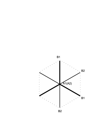
The index denotes the layer index. In Fig. 1 the relative positions of two triangular sublattices, and , for the lattice 1, and and , for the lattice 2 are illustrated. In Eq.(43) is the hopping energy between nearest neighbor C (carbon) atoms in the case of the bilayer graphene in each layer, and is the same energy for hopping between the layers. The on-site creation (annihilation) operators, , are for the electrons in the sublattice of the layer with spin , and for the electrons in the sublattice , is the on-site number operator, and is the chemical potential. ’s are defined as , , and , and , is the distance between atoms and is the next to nearest neighbor distance.
We use units such that . By introducing Fourier transforms and etc. and diagonalizing the Hamiltonian we find for the spectrum,
| (44) |
where , and stand for two kinds of branches. Near points, the corners of the hexagonal Brillouin zone, , we have
| (45) |
and in the limit the lower positive and higher negative branch have the folowing dispersion relation,
| (46) |
where and , the Fermi-Dirac velocity. The effective Hamiltonian near points McFa is
| (47) |
and acts on the subspace of (pseudo)spinors
| (48) |
around point , and
| (49) |
around point . can be rewritten as
| (50) |
where and , and ’s are Pauli matrices. The operator encodes the projection of the pseudospin on direction . For eigenstates as
| (51) |
the direction may be interpreted as the direction of the pseudospin vector, with projection (chirality) equal to in the case of , and in the case of . Thus in the case of these eigenstates we see explicitly our previous remark that the pseudospin vector rotates for an angle while vector rotates for half an angle circling the Fermi surface around points. That feature of the solutions of the free problem leads to non-trivial pairing in the orbital part of Cooper pairs as we will see later. This is to be contrasted to the behavior in the monolayer, a single honeycomb lattice, where the rotation of vector is strictly followed by the rotation of the pseudospin vector. It is accompanied by -wave pairing, when special (nearest-neighbor) attractive interactions are applied. In that case although two order parameters are of, , and type we have the trivial (-wave) behavior in the orbital part as we have shown earlier.
As the reader may have noticed we did not include the direct hopping between the atoms of B1 and B2 sublattice. This inclusion is required when we model bilayer graphene McFa , but even there for realistic parameters this does not influence the physics at high electron momenta or strong magnetic fields novbi .
But we will consider nearest-neighbor attractive interactions between electrons on B1 and B2 sublattice. Namely these sublattices by themselves make a honeycomb lattice as we can verify by looking at Fig. 1. Due to the strong hopping between A1 and A2 sublattice the complete low-energy physics is projected onto B1 and B2 sublattice. If the interactions are not too strong they can be simply added to this low-energy subspace. The on-site repulsive interactions can be introduced and we do not expect that will change our conclusions. Therefore the complete Hamiltonian will include nearest-neighbor attractive interactions between electrons on B1 and B2 sublattice as follows,
| (52) |
where . We will assume the spin-singlet pairing among nearest neighbors and apply the BCS ansatz with
| (53) |
the superconducting order parameter. Furthermore we assume one and the same for all nearest neighbors, which due to global gauge (U(1)) transformations on ’s and ’s can be chosen real and positive. The interaction part, , becomes
| (54) |
The order parameter in the momentum space is
| (55) |
Therefore near points , which then describes two -wave like superconducting order parameters in a low-energy effective description. Taking into account the complete low-energy reduction the total BCS Hamiltonian can now be cast in the following form in the momentum space near , ,
| (56) |
where
| (57) |
and, with ,
We will omit the discussion concerning in the neighborhood of and momenta: . This entails operators which combine spin with momenta and spin with momenta , and will not provide any new information for the structure of the ground state wave function or energy dispersion at small momenta. We can simply include these operators at the end in the ground state wave function following symmetry requirements for the spin-singlet pairing.
VI Ground state wave functions of superconducting instabilities
We look for the solution of Eq. (56) in the form of a diagonalized Bogoliubov BCS Hamiltonian,
| (58) |
where and , are new quasiparticles at momentum . For the dispersions we have:
| (59) |
where . We define a general solution as
| (60) |
Next we have to solve the Bogoliubov - de Gennes (BdG) equations, which follow from the following condition,
| (61) |
We need to diagonalize the following matrix, , that comes out of Eq. (61):
| (62) |
From this matrix eigenvalue problem we obtain energies of the Bogoliubov quasiparticles,
| (63) |
where stands for the particle and hole branches respectively for two kinds of excitations and . The eigenvectors of matrix (after normalization) enter the following expressions in the long-distance limit for Bogoliubov quasiparticles :
| (64) |
and
| (65) |
and quasiholes:
| (66) |
and
| (67) |
for the Bogoliubov solution near point , where we denoted and .
It is helpful to introduce the creation and annihilation operators of states of definite chirality or projection of the pseudospin along the vector; we denote by positive projection, and by negative projection:
| (68) | |||
| (69) | |||
| (70) | |||
| (71) |
Notice that the states are defined up to a phase factor according to the definitions in Eq.(51), and that in the states around point the roles of electrons in different layers are interchanged. We may then define their superpositions,
| (72) | |||
| (73) |
Then we can rewrite Bogoliubov operators as:
| (74) | |||
| (75) | |||
| (76) | |||
| (77) |
with , and find that the wave function, ,
| (78) |
is annihilated by quasiparticle annihilation operators, , and by quasihole creation operators, . Therefore the new ground state is
| (79) |
where we explicitly introduced the sector that couples momenta around with spin and momenta around with spin by enforcing the explicit spin-singlet pairing which we introduced at the beginning.
From the structure of the ground state wave function for spin-singlet pairing in Eq.(79) we find that electrons pair between and point have the same pseudospin and therefore we have two distinct Cooper pairings for two orthogonal pseudospin states, which we denoted by and . Each pair has a -wave pairing in the orbital part and, as we work with a time-reversal invariant system, two distinct Cooper pairings are accompanied by two distinct, and , symmetries in the orbital part. Each Cooper pair is antisymmetric under spin exchange, valley exchange, and exchange in the orbital part and symmetric under sublattice (pseudospin) exchange. Therefore the ground state wave function in Eq.(79) describes a Cooper-paired collection of fermions -electrons on the bilayer honeycomb lattice with unconventional -wave pairing.
The non-trivial (non--wave) pairing cannot be eliminated with a gauge transformation. To preserve the form of the free part of the Hamiltonian any gauge transformation should be and , and and , and if we rewrite in terms of these operators
| (80) |
we see that by this gauge transformation we cannot eliminate simultaneously the angular dependence in the two types of Cooper -wave pairings.
Next we will discuss the spinless case. We will assume that all electron spins are polarized and that . In this case the Bogoliubov problem in Eq.(56) for the spin-singlet pairing transforms into a similar one with and and the matrix becomes as follows,
The problem around the point is a copy of the problem around . We find the following eigenvalues for the Eq.(61),
| (81) |
where stands for the particle and hole branches respectively for two kinds of excitations and . The eigenvectors enter the following expressions in the long-distance limit for Bogoliubov quasiparticles :
| (82) |
and
| (83) |
and quasiholes:
| (84) |
and
| (85) |
Introducing as in the spin-singlet case the following pseudospin operators:
| (86) | |||||
| (87) |
we can rewrite the eigenvectors as follows,
| (88) | |||
| (89) | |||
| (90) | |||
| (91) |
Similarly as in the spin-singlet case we can find that the ground state wave function can be expressed as
| (92) | |||||
| (93) |
The Cooper pairs are symmetric under valley and sublattice (pseudospin) exchange and antisymmetric under exchange in the orbital part. We have two kinds of Cooper pairs with underlying and symmetry.
VII The nature of pairing phases
VII.1 Gaps and possible nodes
In Ref. blh, the case of spin-singlet pairing in the monolayer was thoroughly discussed. A topological phase structure was described with four (due to valley and spin) Dirac edge modes. This is consistent with our previous calculations of the ground state wave function that has explicit -wave dependence for (chemical potential). Here we extended ground state calculations to the spin-singlet and spin-triplet case of the bilayer. It is appropriate to ask the question raised in Ref. blh, for spin-singlet and spin-triplet monolayer case: Are these phases truly gapped or there are nodes for some ’s in the bulk spectrum ? In the same reference it was found that in the spin-triplet case, as opposed to the spin-singlet case, there are nodes in space at which gap is equal to zero. We will find a similar situation in the bilayer case, except that in the case of spin-singlet pairing there is a critical value for chemical potential above which we have a truly gapped - topological phase. (The triplet case just as in the monolayer analysis in Ref. blh, has nodes in the bulk spectrum.)
It is not hard, by repeating the approach of Ref.McFa, , to find expressions for the matrix, , that enters BdG equations in both cases for general (not low) momentum . They are
| (94) |
where and and stand for spin-singlet and spin-triplet case respectively. We look for the zeros of Bogoliubov quasiparticle energies, expressed in the low limit in Eq.(63) and Eq.(81), when . With no low momentum limit, from Eq.(94), their expressions are,
| (95) |
where we used shorthand notation taking , and and correspond to the spin-singlet and spin-triplet case respectively. We assume that is small with respect to so that possible nodes can be only near Fermi surface defined by . Equating and to zero is equivalent to the following condition,
| (96) |
where is the phase of - complex number in general. If we assume that we work with ’s near Fermi surface we have approximately
| (97) |
where is defined by as a small depature from the Fermi surface value. Therefore we can approximate that for possible nodes near Fermi surface in the case of spin-singlet pairing is imaginary i.e. and in the case of spin-triplet pairing is real i.e. .
It is not hard to find nodes in the spin-triplet case. From the definition,
| (98) |
we can recognize that possible positions of nodes can be restricted to , because in that case takes real values; . Then in our approximation from Eq.(97) and definition we have
| (99) |
and that with defines a position of a single node. Therefore the existence of this node (and other related by symmetry) tell us that this phase is likely to be gapless even in the bulk and can not represent a topological phase.
In the spin-singlet case, if we rescale the momentum as in Eq.(98), the condition that is purely imaginary demands that
| (100) |
Then
| (101) |
Expressed differently as
| (102) |
this leads to the conclusion that for large enough i.e. chemical potential this equation does not have a solution for . We find that for no solution exists. Therefore for large enough chemical potential we can have a spin-singlet topological phase i.e. a phase with no gapless bulk excitations.
VII.2 Edge modes
To further examine the topological nature of the spin-singlet phase we will derive its edge modes. With respect to the lattice structure we will consider a particular geometry where the system, defined on a half-plane, has the edge at . We remind the reader that we use the convention in which vectors are along axis. This choice of boundary corresponds to so-called armchair boundary condition for which we require that the solutions of BdG equations vanish at .
We will consider BdG equations in the low limit around points, neglect terms quadratic in , and employ the substitution to get their form in the real space; due to the symmetry of the problem we seek solutions in the form and keep the dependence. The expression for BdG matrix at momentum is
| (103) |
and at momentum ,
| (104) |
and we immediately see a reduction of the problem to four sets of equations with the substitution . If we denote by
| (105) |
a form of a solution, where we used and to denote in a shorthand notation pseudospin (compare with Eq.(60) where the same symbols were used for real spin), we have four sets of equations of similar form. For example, one set at point is:
| (106) |
Just as argued in Ref. rg, in the case of a simple -wave superconductor, when and we have a zero mode, . The difference here is that and carry opposite valley indexes and we cannot construct Majorana Bogoliubov quasiparticle with them, but only a Dirac one. For we find a chiral (unidirectional) mode: . Considering analogous equation for and at point we get an additional solution with the same chirality (the same direction of ), but these two solutions enter the boundary condition which requires that vanishes at the boundary. Therefore one solution with is
| (107) |
where . The other, with and , we find in analogous way. Therefore, we find, as expected from the ground state wave function in Eq.(79), two (Dirac) solutions with opposite directions of motion along the edge that carry opposite pseudospin. In addition, due to the spin degree of freedom we expect doubling of modes i.e. in total two Dirac modes in each direction.
VIII Discussion and conclusions: Superconductivity on bilayer honeycomb lattice
We do not have to go into a discussion of topological invariants to recognize that ground states for spin-singlet pairing, Eq. (79), and for spin-triplet pairing, Eq.(92), may represent ground states of trivial topological superconductors; spin and valley degree of freedom induce the doubling of Majorana modes that may follow rg from -wave pairing in the orbital part. Nevertheless these models of superconductors are interesting in their own right due to the presence of the -wave pairings in the orbital part. In the case of spin-singlet pairing we found that there are no gapless bulk excitations for large enough chemical potential and this phase can represent a trivial topological superconductor.
In deriving ground state wave functions, in the spin-singlet and spin-triplet case, we assumed validity of small expansion around . In a strict sense this requires that is in the same neighborhood where we can approximate dispersion relations i.e. either effective hopping (Fermi velocity) is large or chemical potential is small. We also allowed the possibility that minima or even nodes (in the spin-triplet case) in the spectra of the superconductors can be away from , around . In the cases of the trivial topological superconductors, on the monolayer and bilayer honeycomb lattice, this seems completely justified in the view of their edge spectrum (see also blh ). In the cases of gapless spin-triplet superconductors derived ground state wave functions, though we are inclined to associate them with topological phases, may describe these critical states comment . We find that only if we apply bias to the bilayer larger than its chemical potential we can not apply the BdG program around in the way we described in the paper. (We remind the reader that with the bias the energy minima of the noninteracting problem shift from at points to nonzero ’s.)
The attractive interactions that we need for the realization of the paired ground states and phases may well be within the reach of future experiments. In the case of a single honeycomb lattice the interactions may be induced by chemically doping the graphene via metal coating ucho or trapping fermionic atoms in a honeycomb optical lattice zhu .
To conclude, in the second part of this paper we derived ground state wave functions for the superconductivity on the bilayer honeycomb lattice (with strong interlayer coupling) induced by attractive interactions between sites that participate in a low-energy description. As is well-known, without these interactions, free electrons are described by a Dirac equation with a quadratic dispersion. This unusual feature, similarly to 3He - B phase, leads to the description with two kinds of Cooper pairs, with and pairing, in the presence of the attractive interactions. This is expressed in Eq.(79) in the case of the spin-singlet pairing. Due to the spin degree of freedom we find doubling of two chiral Dirac modes with opposite pseudospin on the edge of this spin-singlet superconductor - a trivial topological superconductor.
IX Acknowledgment
This work was supported in part by the Ministry of Science and Technological Development of the Republic of Serbia, under project No. ON171017.
References
- (1) K.S. Novoselov, A.K. Geim, S.V. Morozov, D. Jiang, Y. Zhang, S.V. Dubonos, I.V. Georgieva, and A.A. Firsov, Science 306, 666 (2004).
- (2) H.B. Heersche, P. Jarillo-Herrero, J.B. Oostinga, L.M.K. Vandersypen, and A.F. Morpurgo, Nature 446, 56 (2007).
- (3) B. Uchoa and A.H. Castro Neto, Phys. Rev. Lett. 98, 146801 (2007).
- (4) A.M. Black-Schaffer and S. Doniach, Phys. Rev. B 75 134512 (2007).
- (5) B. Roy and I. Herbut, Phys. Rev. B 82, 035429 (2010).
- (6) G. Moore and N. Read, Nucl.Phys. B 360, 362 (1991).
- (7) N. Read and D. Green, Phys. Rev. B 61, 10267 (2000).
- (8) C. Nayak, S.H. Simon, A. Stern, M. Freedman, and S. Das Sarma, Rev. Mod. Phys. 80, 1083 (2008).
- (9) For an analysis of possible order parameters and solutions see D. Poletti, C. Miniatura, and B. Gremaud, arXiv:1006.3179
- (10) J.R. Schrieffer, Theory of Superconductivity, p. 42, (Addison-Wesley, 1988).
- (11) X.-L. Qi, T.L. Hughes, S. Raghu, and S.-C. Zhang, Phys. Rev. Lett. 102, 187001 (2009).
- (12) T.H. Hansson, V. Oganesyan, and S.L. Sondhi, Ann. Phys. 313, 497 (2004).
- (13) C.L. Kane and E.J. Mele, Phys. Rev. Lett. 95, 226801 (2005)
- (14) M.V. Milovanović, Journal of Research in Physics, Novi Sad, in press
- (15) E. McCann and V.I. Falko, Phys. Rev. Lett. 96,086805 (2006).
- (16) K.S. Novoselov, E. McCann, S.V. Morozov, V.I. Falko, M.I. Katsnelson, U. Zeitler, D. Jiang, F. Schedin, A.K. Geim, Nature Physics 2, 177 (2006).
- (17) D.L. Bergman and K. Le Hur, Phys. Rev.B 79, 184520 (2009).
- (18) This may be compared with the case of Pfaffian, which can be associated with the transition between 331 state and Fermi liquid state in the context of fractional quantum Hall effect as in Z. Papić, M.O. Goerbig, N. Regnault, and M.V. Milovanović, Phys. Rev. B 82, 075302 (2010).
- (19) S.-L. Zhu, B. Wang, and L.-M. Duan, Phys. Rev. Lett. 98, 260402 (2007).