Decoherence-free dynamics of quantum discord for two correlated qubits in finite-temperature reservoirs

Abstract

We investigate decoherence-free evolution (DFE) of quantum discord (QD) for two initially-correlated qubits in two finite-temperature reservoirs using an exactly solvable model. We study QD dynamics of the two qubits coupled to two independent Ohmic reservoirs when the two qubits are initially prepared in $X$-type quantum states. It is found that reservoir temperature significantly affects the DFE dynamics. We show that it is possible to control the DFE and to prolong the DFE time by choosing suitable parameters of the two-qubit system and reservoirs.

I INTRODUCTION

It is well known that quantum entanglement RMP73(09)00565 ; RMP77(05)00633 ; RMP73(01)00357 ; physrep04 ; physrep02 ; physrep05 ; RMP81(09)00865 , is a distinctive quantum feature of quantum correlations, but not the only one. In order to capture nonclassical correlations, several measures of correlations have been proposed in the literature JPA34 ; oh3PRL89 ; GPWPRA72 ; SLPRA77 ; VedPRL104 ; DLZPRL101 ; zerekdMD . Among them, quantum discord (QD) has received considerable attention PRL105(10)020503 ; PRL100(08)090502 ; JPA41(08)205301 ; Lidar102 ; DGPRA79 ; Yuan43 , which quantifies the quantumness of correlations between two partitions in a composite state zurekPRL88 . The QD, which measures general nonclassical correlations including entanglement, is defined as the mismatch between two quantum analogues of classically equivalent expression of the mutual information. For pure entangled states, all nonclassical correlations which can be characterized by the QD are identified as entanglement. For mixed states, the entanglement can not totally describe nonclassical correlation. Even for some separable states, although there is no entanglement between these two parts, the QD is nonzero, which indicates the presence of nonclassical correlations. And compared to classical counterparts, such separable states can also improve performance in some computational tasks Datta100 ; LBAW101 . In fact, Nonclassical correlation described by the QD can be considered as a more universal quantum resource than quantum entanglement in some sense, and the QD offers new prospects for quantum information processing.

Any realistic quantum system will inevitably interact with the surrounding environment, which causes the rapid destruction of crucial quantum properties. Therefore, besides the characterization and quantification of correlations, an interesting and crucial issue is the behavior of correlations under decoherence. The QD dynamics have been widely studied by using models where qubits interacts in zero-temperature reservoirs Wang2009 ; MWPRA81 ; Yuan43 ; Piilo2010 ; VedPRA80 ; cel ; xu1 ; xu2 . Moreover, QD is more robust than the entanglement against decoherence WSPRA80 ; FWPRA81 ; FAPRA81 ; MWPRA81 . Also, unlike the entanglement, which exhibits sudden death  Yu2004 ; Bellomo2007 ; Choi2007 ; opez2008 ; Qasimi2008 ; Maniscalco2008 , the QD displays the sudden-transition phenomenon from a decoherence-free-evolution (DFE) to a decoherence-evolution regime in the dynamic evolution Piilo2010 ; VedPRA80 ; cel , and the inital QD remains unchanged in the DFE regime. The This sudden-change phenomenon have been demonstrated in recent experiments xu1 ; xu2 . It is of significant interest to prolong the DFE time of the QD in quantum information science since quantum information processing favors the long DFE time of the QD in the dynamic evolution. In this paper, we study the possibility of prolonging the DFE time of the QD by investigating the DFE dynamics of initially-correlated two qubits in two finite-temperature reservoirs. We shall show that the DFE time of the QD can be controlled by choosing initial-state parameters of the two qubits, reservoir parameters, and qubit-reservoir interactions.

This paper is organized as follows: In Sec. II, we present our physical model and study its solution. In Sec. III, we study the DFE dynamics of the QD to indicate the possibility of prolong the DFE time of the QD by investigating QD dynamical behaviors of the two qubits in finite-temperature reservoirs for certain initially prepared $X$-type states. The effects of the temperature, the initial-state parameters, the system-reservoir coupling on QD are studied in Sec. IV. Finally, we conclude this work in the last section.

II the model and its solution

The total system we consider is shown in Fig. 1, including a pair of noninteracting qubits A and B in two independent heat baths, respectively. The energy separation between the excited state $\left|e\right\rangle$ and ground state $\left|g\right\rangle$ of qubits is denoted by $\Omega_{i}$ ($i=A,B$). Atoms A and B are coupled individually to its thermal bath with temperature $T_{a}$ and $T_{b}$ respectively. Here, each bath is modelled as an infinite number of harmonic oscillators with frequencies $\omega_{ak}$ and $\omega_{bk}$, which couple to the relevant electronic degrees of freedom of $i$-th qubit via the coupling constants $g_{ik}$. The Hamiltonian of the total system including the two qubits and the environment is composed of three parts

$$H=H_{S}+H_{B}+H_{SE},$$ (1)

where Hamiltonians of the system and baths are given by

$$H_{S}=\frac{\Omega_{A}}{2}{\sigma}_{A}^{z}+\frac{\Omega_{B}}{2}{\sigma}_{B}^{z},$$ (2)

$$H_{B}=\sum_{k}\hbar\left(\omega_{ak}{a}_{k}^{{\dagger}}{a}_{k}+\omega_{bk}{b}_{k}^{{\dagger}}{b}_{k}\right),$$ (3)

where ${\sigma}_{i}^{z}$ is the standard diagonal Pauli matrix, and ${a}_{k}^{{\dagger}}$(${b}_{k}^{{\dagger}}$) and ${a}_{k}$(${b}_{k}$) are the creation and annihilation operators for a oscillator in $k$the mode, obeying the bosonic commutation relation. The system-bath interaction Hamiltonian is given by

$$H_{SE}=\sum_{k}\hbar\left({\sigma}_{A}^{z}g_{Ak}{a}_{k}+{\sigma}_{B}^{z}g_{Bk}{b}_{k}+{\texttt{h.c.}}\right).$$ (4)

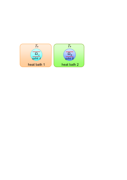
Figure 1: (Color online) Schematic of a pair of noninteracting qubits A and B with energy separations $\Omega_{A}$ and $\Omega_{B}$ under the influence of two independent environments with temperature $T_{a}$ and $T_{b}$.

The bilinear interaction between the system and the bath in $H_{SB}$ indicates that the atomic inverse operator ${\sigma}_{i}^{z}$ commutates with Hamiltonian $H$, i.e. $\left[\sigma_{i}^{z},H\right]=0$. In the rotating frame with respect to Hamiltonian $H_{S}+H_{B}$, the interaction Hamiltonian reads

$$\tilde{H}\left(t\right)=\sum_{k}\hbar\left(g_{Ak}e^{-i\omega_{ak}t}{\sigma}_{A}^{z}{a}_{k}+g_{Bk}e^{-i\omega_{bk}t}{\sigma}_{B}^{z}{b}_{k}+{\texttt{h.c.}}\right),$$ (5)

Equation (5) indicates that the state of the environment will be sensitive to the values of $\sigma_{i}^{z}$. The commutation $\left[H_{S},H_{SE}\right]=0$ suggests that no energy exchanges between qubit and bath, i.e., energy of the system $S$ is conservative BBcontrol ; Kuang1999 . Therefore, the model describes a purely decohering mechanism. The evolution operator generated by the effective Hamiltonian (5) is given by $U\left(t\right)=U_{a}\left(t\right)U_{b}\left(t\right)$ with

$$U_{i}(t)=\exp\left\{\frac{\sigma_{i}^{z}}{2}\sum_{k}\left[X_{k}\xi_{Xk}^{\ast}\left(t\right)-\texttt{h.c.}\right]\right\}$$ (6)

where $\xi_{Xk}\left(t\right)=\frac{2g_{Xk}}{\omega_{Xk}}\left(1-e^{i\omega_{Xk}t}\right)$. Here, $X=a(b)$ when $i=A(B)$. The analytical solution of this model allows us to study behaviors of these correlations under the action of decoherence without any approximations.

In order to show how decoherence affects the correlations in this two-qubit composite system, we assume that the initial state of the two baths is a thermal state denoted by the following density operator

$$\rho_{E}\left(0\right)=\prod_{X,k}\left(1-e^{-\beta_{X}\hbar\omega_{Xk}}\right)e^{-\beta_{X}\hbar\omega_{Xk}X_{k}^{{\dagger}}X_{k}}$$ (7)

where $\beta_{X}=\left(k_{B}T_{X}\right)^{-1}$, and the initial state of the two qubits is denoted by the density operator $\rho_{S}\left(0\right)$, the total system is assumed as a product state of these two initial states $\rho\left(0\right)=\rho_{S}\left(0\right)\otimes\rho_{E}\left(0\right)$. By tracing out over the state of the environment, we can obtain the quantum state of the two qubits at any time

$$\rho_{S}\left(t\right)=\texttt{Tr}_{E}\left[U^{{\dagger}}\left(t\right)\rho\left(0\right)U\left(t\right)\right].$$ (8)

In the Hilbert space spanned by the two-qubit product state basis $\left\{\left|gg\right\rangle,\left|ge\right\rangle,\left|eg\right\rangle,\left|ee\right\rangle\right\}$, the density operator $\rho_{S}\left(t\right)$ loses its off-diagonal terms as a result of the interaction with the environment $E$. The elements of the density operator $\rho_{S}\left(t\right)$ can be exactly obtained as

$$\rho_{(l_{A},l_{B})(j_{A},j_{B})}(t) = \rho_{(l_{A},l_{B})(j_{A},j_{B})}(0)$$ (9)

$$\times\exp{[(\delta_{l_{A},j_{A}}-1)\Gamma_{A}\left(t\right)]}$$

$$\times\exp{[(\delta_{l_{B},j_{B}}-1)\Gamma_{B}\left(t\right)}],$$

where $l,j=e,g$ and ${\delta_{l,j}}$ is the Kronecker delta function. Here, we note that no approximation is employed. Equation (9) shows that diagonal terms of the reduced density matrix $\rho_{S}\left(t\right)$ remain in the initial value, however, the off-diagonal terms vary with the time evolution. The two time-dependent decohering factors are defined by

$$\Gamma_{i}\left(t,0\right)=\sum_{X,k}\frac{\left|\xi_{X,k}\left(t\right)\right|^{2}}{2}\coth\left(\frac{\hbar\beta_{X}\omega_{Xk}}{2}\right),$$ (10)

which are two real-value functions completely to characterize the two-qubit dynamics in the decohering process.

Since the states in the reservoir are very dense (continuum), we can take the continuum limit to convert the summation over $k$ into an integral with respect to $\omega_{X}$. Then the properties of environment are described by the reservoir spectral density

$$J\left(\omega_{X}\right)=\sum_{X,k}\delta(\omega_{X}-\omega_{X,k})\left|g_{X,k}\right|^{2}.$$ (11)

With these replacements, the two decohering factors in Eq. (10) become

$$\Gamma_{i}\left(t\right) = 8\int_{0}^{\infty}d\omega_{X}\frac{J\left(\omega_{X}\right)}{\omega^{2}_{X}}\coth\left(\frac{\hbar\beta_{X}\omega_{X}}{2}\right)$$

$$\times\sin^{2}\left(\frac{\omega_{X}t}{2}\right).$$

III DFE dynamics of the QD for two initially correlated qubits

In this section we study DFE dynamics of the QD for the two initially correlated qubits in the two independent finite-temperature reservoirs by investigating the QD dynamics under decoherence. The total correlations between two qubits A and B described by a bipartite quantum state $\rho_{AB}=\rho_{S}$ are generally measured by quantum mutual information

$$\mathcal{I}\left(\rho_{S}\right)=S\left(\rho_{A}\right)+S\left(\rho_{B}\right)-S\left(\rho_{S}\right),$$ (13)

where $S\left(\rho\right)=-\text{Tr}(\rho\log\rho)$ is the von Neumann entropy of density matrix $\rho$, $\rho_{A}\left(\rho_{B}\right)$ is the reduced density operators for subsystem A(B). Quantum mutual information contains quantum correlation $\mathcal{D}\left(\rho_{S}\right)$ and classical correlation $\mathcal{C}\left(\rho_{S}\right)$JPA34 ; VedPRL90 ; VedPRA80 . Quantum correlation $\mathcal{D}\left(\rho_{S}\right)$ can be quantified by the QD zerekdMD ; zurekPRL88 , which is defined by the discrepancy between quantum versions of two classically equivalent expressions for mutual information

$$\mathcal{D}\left(\rho_{S}\right)=\mathcal{I}\left(\rho_{S}\right)-\mathcal{C}\left(\rho_{S}\right)\text{,}$$ (14)

where the classical correlation $\mathcal{C}\left(\rho_{S}\right)$ is defined as the maximum information about one subsystem $\rho_{i}$, which depends on the type of measurement performed on the other subsystem. For a local projective measurement $\Pi_{k}$ performed on the subsystem $B$ with a given outcome $k$, we denote

$$p_{k}=\text{Tr}_{AB}[(I_{A}\otimes\Pi_{k})\rho_{S}(I_{A}\otimes\Pi_{k})].$$ (15)

as the probability, where $I_{A}$ is the identity operator for the subsystem $A$. Then the classical correlation reads

$$\mathcal{C}(\rho_{S}) = \max_{\{\Pi_{k}\}}\left[S(\rho_{A})-\sum_{k}p_{k}S(\rho_{A}^{(k)})\right]$$

$$= S(\rho_{A})-\min_{\{\Pi_{k}\}}\left[\sum_{k}p_{k}S(\rho_{A}^{(k)})\right],$$

where the maximum is taken over the complete set of orthogonal projectors $\left\{\Pi_{k}\right\}$ and

$$\rho_{A}^{(k)}=\frac{1}{p_{k}}\text{Tr}_{B}\left[\left(I_{A}\otimes\Pi_{k}\right)\rho(I_{A}\otimes\Pi_{k})\right]$$ (17)

is the reduced density matrix of subsystem $A$ after obtaining the measurement outcome $k$, which is normalized.

Let us first find the analytical expression for the density operator of two qubits at time $t$. We assume the two qubits are initial in a class of states with maximally mixed marginals, which is described by the $X$-structured density operator

$$\rho_{S}\left(0\right)=\frac{1}{4}\left(I_{AB}+\underset{j=1}{\overset{3}{\sum}}c_{j}\sigma_{A}^{j}\otimes\ \sigma_{B}^{j}\right).$$ (18)

Here, the coefficients $c_{j}$ with real constants satisfy the condition that $\rho_{S}(0)$ is positive and normalized, and $I_{AB}$ is the identity operator of the two qubits. Obviously, such states $\rho_{S}\left(0\right)$ are general enough to include states such as the Werner states and the Bell states.

Using the results obtained in Eq.(9), the density matrix of two qubits at time $t$ has the following analytical expression

$$\rho_{S}\left(t\right)=\frac{1}{4}\left(\begin{array}[]{cccc}1+c_{3}&0&0&\tilde{\alpha}^{\ast}\\ 0&1-c_{3}&\tilde{\gamma}^{\ast}&0\\ 0&\tilde{\gamma}&1-c_{3}&0\\ \tilde{\alpha}&0&0&1+c_{3}\end{array}\right),$$ (19)

where $\tilde{\alpha}=\alpha(t)e^{-i(\Omega_{A}+\Omega_{B})t}$ and $\tilde{\gamma}=\gamma(t)e^{i(\Omega_{B}-\Omega_{A})t}$ with,

$$\alpha(t) = (c_{1}-c_{2})D_{A}(t)D_{B}(t),$$ (20a)

$$\gamma(t) = (c_{1}+c_{2})D_{A}(t)D_{B}(t),$$ (20b)

where $$D_{i}(t)=\exp\left[-\Gamma_{i}\left(t\right)\right] \rho_{i}\left(t\right)=I_{i}/2 i=A,B \rho_{S}\left(t\right)$$ are decohering functions. Since the reduced density matrix of subsystem , and the eigenvalues of the two-qubit density operator can be exactly calculated from Eq.(19) with the following expressions

$$\lambda_{1,2} = \frac{1}{4}\left(1+c_{3}\mp\alpha\right)$$ (21a)

$$\lambda_{3,4} = \frac{1}{4}\left(1-c_{3}\mp\gamma\right),$$ (21b)

quantum mutual information can be written as

$$\mathcal{I}\left(\rho_{S}\right)\ =2+{\sum_{i=1}^{4}}\lambda_{i}\log\lambda_{i}.$$ (22)

Now, we turn to calculating the classical correlation $\mathcal{C}(\rho_{S})$ defined in Eq. (III). In the Hilbert space spanned by $\left\{\left|e\right\rangle,\left|g\right\rangle\right\}$, any two orthogonal states $\left|\mathbf{0}\right\rangle$ and $\left|\mathbf{1}\right\rangle$ can be represented as a unitary vector on the Bloch sphere

$$\left|\mathbf{0}\right\rangle =\cos\theta\left|g\right\rangle+e^{i\phi}\sin\theta\left|e\right\rangle,$$ (23a)

$$\left|\mathbf{1}\right\rangle =e^{-i\phi}\sin\theta\left|g\right\rangle-\cos\theta\left|e\right\rangle,$$ (23b)

with $$0\leq\theta\leq\pi/2 0\leq\phi\leq 2\pi B \Pi_{\mathbf{0}}=\left|\mathbf{0}\right\rangle\left\langle\mathbf{0}\right| \Pi_{\mathbf{1}}=\left|\mathbf{1}\right\rangle\left\langle\mathbf{1}\right| p_{\mathbf{0}}=p_{\mathbf{1}}=1/2 A k$$ and . Therefore, for a local measurement performed on the subsystem , a complete set of orthogonal projectors contains two elements and with the probability . After the two project measurements the reduced density operator of subsystem with an outcome reads

$$\rho_{A}^{\left(k\right)}=\frac{1}{4}\left(\begin{array}[]{cc}2(1-c_{3}\cos(2\theta))&\left(-1\right)^{k}\epsilon\sin(2\theta)\\ \left(-1\right)^{k}\epsilon^{\ast}\sin(2\theta)&2(1+c_{3}\cos(2\theta))\end{array}\right)$$ (24)

where we have introduced the following parameter

$$\epsilon=\alpha e^{i\left[(\Omega_{A}+\Omega_{B})t-\phi\right]}+\gamma e^{i\left[(\Omega_{A}-\Omega_{B})t+\phi\right]}\text{.}$$ (25)

Making use of Eq. (24), it is straightforward to calculate the classical correlation with the following expression Yuan43

$$\mathcal{C}\left(\rho_{S}(t)\right)=\overset{2}{\underset{n=1}{\sum}}\frac{1+(-1)^{n}\chi(t)}{2}\log_{2}\left[1+(-1)^{n}\chi(t)\right],$$ (26)

where

$$\chi(t)=\max\left[\left|c_{3}\right|,(|\alpha(t)|+|\gamma(t)|)/2\right],$$ (27)

which depends on the relation between the coefficients $c_{j}$ of the initial state in Eq.(18) and the dynamic parameters defined by Eq. (22). From Eq. (27) we can see that: (i) If $|c_{3}|>(|\alpha|+|\gamma|)/2$, we have $\chi(t)=\left|c_{3}\right|$; (ii) If $|c_{3}|<(|\alpha|+|\gamma|)/2$, we have $\chi(t)=(|\alpha|+|\gamma|)/2$.

Then the QD between the two qubits can be written as

$$\mathcal{D}(\rho_{S}(t))=2+\sum_{i=1}^{4}\lambda_{i}\log_{2}\lambda_{i}-\mathcal{C}(\rho_{S}(t)).$$ (28)

In order to clearly understand the QD dynamics of two qubits in two independent reservoirs, we consider the case of $c_{1}=1$, $c_{2}=-c_{3}$, and $\ \left|c_{3}\right|<1$. In this case, from Eq. (27) we can obtain

$$\chi(t)=\max[|c_{3}|,D_{A}(t)D_{B}(t)],$$ (29)

where the two decohring functions are given by

$$D_{i}(t)=(1+\omega_{ic}^{2}t^{2})^{-\frac{\eta_{i}}{2}}\prod_{n=1}^{\infty}\left[1+\frac{\omega_{ic}^{2}t^{2}}{(1+\hbar\beta_{i}\omega_{ic}n)^{2}}\right]^{-\eta_{i}},$$ (30)

where $i=(A,B)$ and we assume the two reservoirs have the Ohmic spectral density LegRMP59 given by

$$J(\omega_{i})=\eta_{i}\omega_{i}\exp\left(\frac{-\omega_{i}}{\omega_{ic}}\right).$$ (31)

where $\eta_{i}>0$ is the system-reservoir coupling constant, and $\omega_{ic}$ is the high-frequency cut-off.

Taking into account the decohring functions $D_{A}(t)$ and $D_{B}(t)$ decay in the time evolution, making use of Eqs. (21), (26), (28), and (29), we can find the critic time denoted by $t_{p}$ which is given by the condition $D_{A}(t_{p})D_{B}(t_{p})=|c_{3}|$, and we can see that before the critic time, i.e., $t<t_{p}$, the initial QD can remain unchanged in the time evolution while the QD decays after the critic time, i.e., $t>t_{p}$. Therefore, the time $t_{p}$ is the DFE time of the QD. In what follows we calculate explicitly analytical expression of the QD in the whole time evolution to indicate how to control the DFE time of the QD.

In the DFE regime of the QD, i.e., $t<t_{p}$, since $D_{A}(t_{p})D_{B}(t_{p})>|c_{3}|$, we have $\chi(t)=D_{A}(t)D_{B}(t)\equiv D_{A}D_{B}$. Consequently, the classical correlation reads

$$\mathcal{C}(\rho_{S}(t)) = \frac{1}{2}\Omega_{-}(t)\log_{2}\Omega_{-}(t)+\frac{1}{2}\Omega_{+}(t)\log_{2}\Omega_{+}(t),$$

where we have introduced $\Omega_{\pm}(t)=1\pm D_{A}(t)D_{B}(t)$.

Subtracting the classical correlation from the quantum mutual information $\mathcal{I}(\rho_{S})$, we find that the QD is given by

$$\mathcal{D}(\rho_{S}(t))=\sum_{n=0}^{1}\frac{1}{2}[1+(-1)^{n}c_{3}]\log_{2}[1+(-1)^{n}c_{3}],$$ (33)

which is independent of time. Hence, in the regime of $t<t_{p}$ the QD dynamics is decoherence-free, and the initial QD can be preserved.

In the regime of the QD decay, i.e., $t>t_{p}$, since $D_{A}(t)D_{B}(t)<|c_{3}|$, we have $\chi(t)=\left|c_{3}\right|$. The classical correlation is a constant

$$\mathcal{C}(\rho_{S}(t))=\sum_{n=0}^{1}\frac{1}{2}[1+(-1)^{n}c_{3}]\log_{2}[1+(-1)^{n}c_{3}],$$ (34)

then the QD reads

$$\mathcal{D}(\rho_{S}(t)) = \frac{1}{2}\Omega_{-}(t)\log_{2}\Omega_{-}(t)+\frac{1}{2}\Omega_{+}(t)\log_{2}\Omega_{+}(t),$$

which is a decaying function of time.

The above discussion shows that the QD exhibits a sudden change at the critic time $t_{p}$. The QD evolution dynamics displays different behaviors before and after the critic time. The initial QD can be preserved in the regime of $t<t_{p}$ while the QD decays in the time evolution regime of $t>t_{p}$. In what follows we discuss the dependence of the DFE time of the QD upon the initial-state parameters, the system-reservoir coupling, and the reservoir temperature for the case of two equal-temperature reservoirs and the case of two unequal-temperature reservoirs, respectively.

Figure 2: (Color online) 3D diagram of the quantum discord as a function of $\beta$ and $\omega_{c}t$ in the case of two equal-temperature reservoirs under the setting $\eta=0.2$, $c_{1}=1$, and $c_{2}=-c_{3}=0.4$.

III.1 The case of two equal-temperature reservoirs

In this subsection, we assume the two reservoirs are identical, i.e., $\omega_{Ac}=\omega_{Bc}=\omega_{c},\eta_{A}=\eta_{B}=\eta,\beta_{A}=\beta_{B}=\beta$. Then we have $D_{A}(t)=D_{B}(t)=D(t)$.

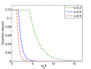
Figure 3: (Color online) Plot of the quantum discord vs the scaled time $\omega_{c}t$ in the case of two equal-temperature reservoirs with the qubit-reservoir coupling $\eta=0.2$ for dash green line, $\eta=0.6$ for solid blue line, $\eta=0.9$ for dash-dot red line. Other parameters are taken as $c_{1}=1$, $c_{2}=-c_{3}$, and $c_{3}=0.4$, and $\beta=5$.

At zero temperature, from Eq. (30) we can explicitly obtain the decohering function with the form $D(t)=(1+\omega_{c}^{2}t^{2})^{-\eta/2}$, which allows us to achieve the expression of the QD preservation time

$$t_{p}=\frac{\sqrt{|c_{3}|^{-1/\eta}-1}}{\omega_{c}},$$ (36)

which indicates that the DFE time depends on the initial-state parameter $c_{3}$, the qubit-bath coupling $\eta$, and the bath parameter $\omega_{c}$. The DFE time increases with the decrease of the initial-state parameter $|c_{3}|$ or/and the decrease of the qubit-bath coupling $\eta$. Moreover, for a set of given parameters ($c_{3},\eta$), the lower the cut-off frequency of the reservoir is, the longer the preservable time will be.

At finite temperatures, we can numerically study the influence of the initial-state parameter, the qubit-bath coupling,the bath parameter, and the bath temperature upon the QD preservation time. In Fig. 2, we have plotted the QD as a function of $\beta$ and $\omega_{c}t$. From Fig. 2 we can see that a sudden change of the QD occurs at the critic time of $t=t_{p}$, the initial QD can be preserved in the time evolution regime of $0\leq t\leq t_{p}$. However, The QD decays in the time evolution regime of $t>t_{p}$. We can also see that the decrease of the bath temperature prolongs the DFE time of the initial QD and slows the decay rate of the QD.

Fig. 3 shows the effect of the qubit-reservoir coupling $\eta$ on the QD dynamics. From Fig. 3 we can see that the DFE time of the initial QD $t_{p}$ increases and the QD decay after the time $t_{p}$ becomes slower when the system-reservoir coupling constant $\eta$ decreases. Hence, we can conclude that the smaller the qubit-reservoir coupling $\eta$, the more robust the QD against decoherence.

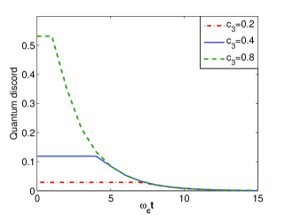
Figure 4: (Color online) Plot of the quantum discord vs the scaled time $\omega_{c}t$ in the case of two equal-temperature reservoirs with the initial-state parameter $\left|c_{3}\right|=0.2$ for dash green line, $\left|c_{3}\right|=0.4$ for solid blue line, and $\left|c_{3}\right|=0.8$ for dash-dot red line. Other parameters are taken as $\eta=0.2$, $c_{1}=1$, $c_{2}=-c_{3}$, and $\beta=5$.

The effect of the initial-state parameter $\left|c_{3}\right|$ on the QD dynamics is shown in Fig. 4 where we have plotted the time evolution of the QD for $\beta=5$. From Fig. 4 we can see that one can make the DFE time of the initial QD $t_{p}$ longer by decreasing the magnitude of the initial-state parameter $|c_{3}|$.

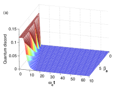
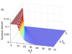
Figure 5: (Color online) 3D diagram of the quantum discord as a function of $\beta_{a}$ and $\omega_{c}t$ in the case of two unequal-temperature reservoirs under the setting: $\eta=0.12$, $c_{1}=1$ and $c_{2}=-c_{3}=0.4$ for different value of $\kappa$, (a) $\kappa=0.2$, (b) $\kappa=1$, (c) $\kappa=5$.

III.2 The case of two unequal-temperature reservoirs

In this subsection, we the influence of the temperature difference the QD dynamics when the two reservoirs have different temperature. We suppose that $\omega_{Ac}=\omega_{Bc}=\omega_{c},\eta_{A}=\eta_{B}=\eta$, and the temperature of two reservoirs satisfies the relation $T_{a}=\kappa T_{b}$, i.e., $\beta_{b}=\kappa\beta_{a}$ where $\kappa$ is a parameter to denote the temperature difference between the two reservoirs. In case of two unequal-temperature reservoirs, the QD dynamics is described analytically Eqs. (33) and (35). In Fig. 5, we have plotted the dynamic evolution of the QD with respect to $\beta_{a}$ for different values of the temperature-difference parameter $\kappa$ when the two qubits are initially prepared in the $X$-type state with the state parameters $c_{1}=1$, $c_{2}=-c_{3}$, and $c_{3}=0.4$.

From Fig. 5 we can see that the temperature difference between the two reservoirs does not change the maximal value of the QD but does change the DFE time of the QD in the dynamic evolution. The maximal value of the QD is stable for different temperature-difference parameter $\kappa$ of the two reservoirs. The decay rate of the QD decreases with the increase of the temperature difference parameter $\kappa$ for the given initial state. From Fig. 5 we can also see that the larger the temperature difference parameter $\kappa$, the longer the DFE time $t_{p}$. Therefore, we conclude that the DFE time can be prolonged under certain conditions through the increase of the temperature difference between the two reservoirs.

IV Concluding remarks

In conclusion, we have studied the DFE dynamics of the QD for two qubits in two finite-temperature environments through investigating the QD dynamics of the two qubits coupled to independent reservoirs. We have chosen the initial state of the two qubits to be $X$-type states which is known to exhibit quantum correlations described by the QD. We have shown that reservoir temperature significantly affects the DFE time of the QD. We have also indicated that it is possible to control the DFE dynamics of the two qubits and to prolong the DFE time by choosing suitable parameters of the two-qubit system and their environments. These results shed new light on the QD control which would be a new direction in quantum information processing.

For $X$-type initial states with the state parameters $c_{1}=1,c_{2}=-c_{3}$ and $|c_{3}|<1$, we have investigated the QD dynamics of the two qubits in detail when the two independent reservoirs are Ohmic. In the case of the two zero-temperature reservoirs, we have shown that the DFE time increases with the decrease of the initial-state parameter $|c_{3}|$ or/and the decrease of the qubit-bath coupling $\eta$. Moreover, for a set of given parameters ($c_{3},\eta$), the lower the cut-off frequency of the reservoirs, the longer the DFE time is. In the case of the two nonzero equal-temperature reservoirs, we have indicated that the decrease of the bath temperature can prolong the DFE time of the initial QD and slows the QD decay rate. In the case of the two unequal-temperature reservoirs, it is found that the temperature difference between the two reservoirs does not change the maximal value of the QD but does change the DFE time in the dynamic evolution. The larger the temperature difference parameter, the longer the DFE time $t_{p}$. In this sense, we conclude that the DFE time can be prolonged under certain conditions through the increase of the temperature difference between the two reservoirs.