Tilt-over mode in a precessing triaxial ellipsoid

Abstract

The tilt-over mode in a precessing triaxial ellipsoid is studied theoretically and numerically. Inviscid and viscous analytical models previously developed for the spheroidal geometry by Poincaré [Bull. Astr. 27, 321 (1910)] and Busse [J. Fluid Mech., 33, 739 (1968)] are extended to this more complex geometry, which corresponds to a tidally deformed spinning astrophysical body. As confirmed by three-dimensional numerical simulations, the proposed analytical model provides an accurate description of the stationary flow in an arbitrary triaxial ellipsoid, until the appearance at more vigorous forcing of time dependent flows driven by tidal and/or precessional instabilities.

I Introduction

The flow of a rotating viscous incompressible homogeneous fluid in a precessing container has been studied for over one century because of its multiple applications, such as the motions in planetary liquid cores and the generation of planetary magnetic fields (e.g. Malkus93, ; Tilgner_2005, ). In the spheroidal geometry, the early work of Poincare demonstrated that the flow of an inviscid fluid has a uniform vorticity. Later, viscous effects have been taken into account as a correction to the inviscid modes, in considering carefully the critical regions of the Ekman layer Stewartson_1963 ; Busse ; Greenspan . Indeed, the Poincaré solution is modified by the apparition of boundary layers, and some strong internal shear layers are also created in the bulk of the flow, which do not disappear in the limit of vanishing viscosity Busse . Besides, at high enough precession rates, these shear layers may become unstable malkus68 ; Vanyo_1995 ; Noir_2003 , and in a second transition, the entire flow becomes turbulent: this is the precession instability. These experimental works have been completed by numerical studies in cylindrical, spherical and spheroidal geometries Hollerbach_1995 ; Quartapelle_1995 ; Tilgner_1999a ; Tilgner_2001 ; Noir_2001 , in particular for studying kinematic dynamo models in a spheroidal galaxy Walker_1994 or for geophysical applications Tilgner_1999b ; Lorenzani_2001 ; Lorenzani_2003 ; Schmitt_2004 ; Wu_2009 .

However, in natural systems, both the rotation and the gravitational tides deform the celestial body into a triaxial ellipsoid, where the so-called elliptical (or tidal) instability may take place (see KerswellMalkus ; Lacaze_2004 ; LeBars09 ; Cebron_2010 ; Kerswell_2002 for details on this instability and its geo- and astro-physical applications). The elliptical instability takes place in any rotating fluid whose streamlines are elliptically deformed (see e.g. Waleffe_1990 or LeBars07 ). It comes from a parametric resonance of two inertial waves of the rotating fluid with the tidal (or elliptical) deformation of azimutal wavenumber $m=2$ Kerswell_2002 . Similarly, it has been suggested that the precession instability comes from the parametric resonance of two inertial waves with the forcing related to the precession of azimutal wavenumber $m=1$, which comes from the deviations of the laminar tilt-over base flow from a pure solid body rotation Kerswell_1993 ; Kerswell_1995 ; Lagrange2008 . But it has also been suggested that the precession instability is related to a shear instability of the zonal flows that appear in a precessing container (e.g. Lorenzani_2003, ). Clearly, the precise origin of the precession instability is still under debate, and is beyond the point of the present work. But since tides and precession are simultaneously present in natural systems, it seems necessary to study their reciprocal influence, in presence or not of instabilities. The full problem is rather complex and involves three different rotating frames: the precessing frame, with a period $T_{p}\approx 26000$ years for the Earth, the frame of the tidal bulge, with a period around $T_{d}\approx 27$ days for the Earth, and the container or ’mantle’ frame, with a period $T_{s}\approx 23.93$ hours for the Earth. As a first step towards the full study of the interaction between the elliptical instability and the precession, we consider the particular case where the triaxial ellipsoid is fixed in the precessing frame ($T_{d}=T_{p}$), which allows the theoretical approach to be analytically tractable. We show in figure 1 a sketch of this configuration.

The paper is organized as follow. In section II, Poincaré and Busse analytical models are extended to precessing triaxial ellipsoids. Then in section III, our analysis is validated by comparison with a numerical simulation.

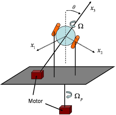
Figure 1: Sketch of the problem under consideration. A hollow solid but deformable spheroid (i.e. ’the mantle’) is filled with liquid and set in rotation at a constant angular velocity $\Omega$ versus its axis $(O{x_{3}})$. The spheroid axis is tilted at the precession angle $\theta$ and fixed on a rotating table, which rotates at the precession rate $\Omega_{p}$. Two fixed rollers aligned with $(O{x_{3}})$ then transform the spheroid into a triaxial ellipsoid by compression along the axis $(O{x_{2}})$, perpendicular to the rotation axis.

II Analytical solution of the flow in a precessing triaxial ellipsoid

In this section, we consider firstly the case of an inviscid fluid and extend the Poincaré model to a precessing triaxial ellipsoid, which allows us to obtain explicit analytical solutions. We then tackle the viscous case in extending the Busse model, following the method of Noir_2003 . As sketched in figure 1, we consider the rotating flow inside a precessing triaxial ellipsoidal container of principal axes $(a_{1},a_{2},a_{3})$. We define $(Ox_{1},Ox_{2},Ox_{3})$ in the frame of the tidal bulge which is also the precessing frame, such that $Ox_{i}$ is along the principal axis $a_{i}$ of the ellipsoidal container and $(O{x_{3}})$ is the mantle rotation axis. We note $\Omega$ the imposed mantle angular velocity and use $\Omega^{-1}$ as a timescale. We also introduce the mean equatorial radius $R_{eq}=(a_{1}+a_{2})/2$, which is used as a lengthscale. Consequently, the problem is fully described by six dimensionless numbers: the eccentricity $\epsilon=(a_{1}^{2}-a_{2}^{2})/(a_{1}^{2}+a_{2}^{2})$, the aspect ratio $a_{3}/a_{1}$, the Ekman number $E=\nu/\Omega R_{eq}^{2}$, where $\nu$ is the kinematic viscosity of the fluid, and the three components of the dimensionless precession vector $\bm{\Omega_{p}}$ in the inertial frame of reference, i.e. the angle $\theta$ between $\bm{\Omega_{p}}$ and $\bm{e_{x_{3}}}$, the angle $\theta_{2}$ between $\bm{\Omega_{p}}$ and $\bm{e_{x_{1}}}$ and the angular precession rate $\Omega_{p}$, which is positive for prograde precession and negative for retrograde precession.

II.1 Inviscid Poincaré tilt-over mode for a triaxial ellipsoid

We look for a base flow solution of the Euler equations, i.e.

$$\frac{\partial\mathbf{u}}{\partial t}+\mathbf{u}\cdot\mathbf{\nabla}\mathbf{u}=-\mathbf{\nabla}p-2\bm{\Omega_{p}}\times\bm{u},$$ (1)

$$\mathbf{\nabla}\cdot\mathbf{u}=0,$$ (2)

inside the triaxial ellipsoid in the precessing frame. In this frame, using the ellipsoid equation

$$\frac{x_{1}^{2}}{a_{1}^{2}}+\frac{x_{2}^{2}}{a_{2}^{2}}+\frac{x_{3}^{2}}{a_{3}^{2}}=1,$$ (3)

we transform the ellipsoidal geometry into a sphere with the transformation $(x^{\prime}_{k})=\left(\frac{x_{k}}{a_{k}}\right)_{k\in(1,2,3)}$ and we write the velocity field in this sphere as

$$(U^{\prime}_{k})=\left(\frac{U_{k}}{a_{k}}\right)_{k\in(1,2,3)}.$$ (4)

As suggested in Poincare , we focus on the so-called ’simple motions’ such that the velocity $\mathbf{U}(U_{1},U_{2},U_{3})$ is described as linear combinations of the coordinates. This hypothesis leads to a solid body rotation in the sphere, i.e. $\mathbf{U^{\prime}}=\bm{\omega^{\prime}}\times\mathbf{r^{\prime}}$, where $\bm{\omega^{\prime}}(\omega^{\prime}_{1},\omega^{\prime}_{2},\omega^{\prime}_{3})$ depends on time a priori. Equation 4 then gives the following velocity field in the ellipsoid:

$$\mathbf{U}=\left(U_{k}\right)_{k\in(1,2,3)}=\left(\frac{a_{k}}{a_{k-1}}\ \omega^{\prime}_{k+1}x_{k-1}-\frac{a_{k}}{a_{k+1}}\ \omega^{\prime}_{k-1}x_{k+1}\right)_{k\in(1,2,3)},$$ (5)

where permutations ${k\in(1,2,3)}$ are used.

Now, we have to find the ’simple motions’ solution of the Euler equations for the rotational part of the flow, taking into account the no-penetration boundary conditions for its irrotational part, which leads to the so-called Poincaré flow. We follow the method of Noir_2000 rather than the lagrangian method of Poincaré which is more laborious. We deduce the rotation rate vector $\bm{\omega}$ from the velocity field (5):

$$\bm{\omega}=\frac{1}{2}\ \mathbf{\nabla}\times\bm{U}=\left(\omega_{k}\right)_{k\in(1,2,3)}=\frac{1}{2}\left(\left(\frac{a_{k-1}}{a_{k+1}}+\frac{a_{k+1}}{a_{k-1}}\right)\ \omega^{\prime}_{k}\right)_{k\in(1,2,3)}.$$ (6)

Note that $\bm{\omega^{\prime}}$ is independent of the space coordinates so that $\bm{\omega}$ is uniform. Taking the rotational of (1), the inviscid equation for $\bm{\omega}$ gives the following three scalar equations:

$$\frac{\mathrm{d}\omega_{k}}{\mathrm{d}t}+(\alpha_{k+1,k}-\alpha_{k-1,k})\ \omega_{k-1}\ \omega_{k+1}=\alpha_{k-1,k}\ \Omega_{p,k-1}\ \omega_{k+1}-\alpha_{k+1,k}\ \Omega_{p,k+1}\ \omega_{k-1}$$ (7)

for permutations $k\in(1,2,3)$, with the coefficients $\alpha_{i,j}=\frac{2}{\eta_{ij}+2}=2\ \frac{\eta_{ji}+1}{\eta_{ji}+2}$ and the different ellipticities $\eta_{ij}=\frac{a_{i}^{2}-a_{j}^{2}}{a_{j}^{2}}$ of the container. The equations for a spheroidal geometry are recovered with $a_{1}=a_{2}$.

We focus on the stationary solutions of the problem. In this particular case, we solve the system (7) analytically, which gives:

$$\omega_{1}=\frac{\omega_{3}}{\beta_{12}}\frac{a_{3}^{2}+a_{2}^{2}}{\gamma_{1}}\ \Omega_{p,1},$$ (8)

$$\omega_{2}=\frac{\omega_{3}}{\beta_{12}}\frac{a_{3}^{2}+a_{1}^{2}}{\gamma_{2}}\ \Omega_{p,2},$$ (9)

where $\beta_{ij}=\frac{a_{i}^{2}+a_{j}^{2}}{2a_{i}a_{j}}=\beta_{ji}$ and $\gamma_{i}=\frac{\omega_{3}}{\beta_{12}}(a_{i}^{2}-a_{3}^{2})+2\ \Omega_{p,3}\ a_{1}\ a_{2}$. The corresponding velocity field writes:

$$U_{1}=a_{1}\ \frac{\omega_{3}}{\beta_{12}}\left(-\frac{x_{2}}{a_{2}}+\frac{2\ a_{1}\ \Omega_{p,2}x_{3}}{\gamma_{2}}\right),$$ (10)

$$U_{2}=a_{2}\ \frac{\omega_{3}}{\beta_{12}}\left(\frac{x_{1}}{a_{1}}-\frac{2\ a_{2}\ \Omega_{p,1}x_{3}}{\gamma_{1}}\right),$$ (11)

$$U_{3}=a_{3}\ \frac{\omega_{3}}{\beta_{12}}\left(\frac{2\ a_{3}\ \Omega_{p,1}x_{2}}{\gamma_{1}}-\frac{2\ a_{3}\ \Omega_{p,2}x_{1}}{\gamma_{2}}\right).$$ (12)

Note that the choice of $\omega_{3}$ is arbitrary here. Actually, $\omega_{3}$ is determined by the boundary (Ekman) layer and thus has to be determined by a viscous study, following for instance the method of Busse , as described in the next section. Note also that this velocity field is divergent for $\gamma_{1}=0$ or $\gamma_{2}=0$: the inviscid study gives two resonances, which correspond to resonance between the frequencies of respectively the precessional forcing and the tilt-over (see Noir_2003 for details). These linear resonances are reached for two specific precession rates (depending on the aspect ratio) which are

$$\Omega_{p,3}=\frac{a_{3}^{2}-a_{i}^{2}}{a_{1}^{2}+a_{2}^{2}}\ \omega_{3}$$ (13)

for $i\in(1,2)$. It is clear that oblate ellipsoids ($a_{1},a_{2}>a_{3}$) have their resonance in the retrograde regime (i.e. in the range $\Omega_{p,3}<0$) whereas prolate ellipsoids ($a_{1},a_{2}>a_{3}$) have their resonance in the prograde regime. Finally, compared to the spheroidal case, an important result here is the apparition of the second resonance created by the equatorial ellipticity of the container.

II.2 Viscous study of the tilt-over mode in a triaxial ellipsoid

Following Busse , it is possible to take into account the viscosity in the study of the flow in a precessing triaxial ellipsoid. Here, we focus on the equivalent method of Noir_2003 , based on the equilibrium between the inertial torque $\bm{\Gamma_{i}}$, the pressure torque $\bm{\Gamma_{p}}$, and the viscous torque $\bm{\Gamma_{v}}$. Keeping the leading terms for these three torques, the general torque balance given in Busse for a steady rotating flow $\bm{q}=\bm{\omega}\times\bm{r}$ in the precessing frame within a volume $V$ with a surface $\Sigma$ writes:

$$\overbrace{2\int_{V}\bm{r}\times(\bm{\Omega_{p}}\times\bm{q})dV}^{\bm{\Gamma_{i}}}=\overbrace{-\oint_{\Sigma}p\bm{r}\times\bm{n}d\Sigma}^{\bm{\Gamma_{p}}}+\overbrace{E\int_{V}\bm{r}\times\nabla^{2}\bm{q}dV}^{\bm{\Gamma_{v}}},$$ (14)

where $\bm{r}$ is the position vector and $\bm{n}$ is the unit vector normal to $\Sigma$ pointing outward (see Noir_2003, ). Now, we have to calculate these terms for a triaxial ellipsoid.

At first order, the pressure gradient equilibrates the centrifugal force, which gives:

$$p=\frac{1}{2}\sum\limits_{\begin{subarray}{c}i=1\end{subarray}}^{3}{\left[(\omega_{i+1}^{2}+\omega_{i-1}^{2})\ x_{i}^{2}-\sum\limits_{\begin{subarray}{c}j=1\\ j\neq i\end{subarray}}^{3}{\omega_{i}\ \omega_{j}\ x_{i}\ x_{j}}\right]}.$$ (15)

Hence in the limit of small ellipticities, i.e. at first order in $\eta=1-a_{3}/a_{1}$ and $\eta_{2}=1-a_{2}/a_{1}$, the pressure torque writes:

$$\bm{\Gamma_{p}}=-\oint p\ \bm{r}\times\bm{n}\ \mathrm{d}\Sigma=\left(\Gamma_{p,k}\right)_{k\in(1,2,3)}=I\left(\begin{array}[]{ccc}(\eta-\eta_{2})\ \omega_{2}\ \omega_{3}\\ -\eta\ \omega_{1}\ \omega_{3}\\ \eta_{2}\ \omega_{1}\ \omega_{2}\\ \end{array}\right),$$ (19)

where I is the moment of inertia in the spherical approximation. Note that the expression of Noir_2003 is recovered for the spheroid (i.e. $a_{1}=a_{2}$ hence $\eta_{2}=0$).

After little algebra, the precessional torque simply writes:

$$\bm{\Gamma_{i}}=I\bm{\Omega_{p}}\times\bm{\omega}.$$ (20)

Finally, the equations (19) and (20) give $\bm{\Gamma_{p}}\cdot\bm{\omega}=0$ and $\bm{\Gamma_{i}}\cdot\bm{\omega}=0$, and thus with the equation (14) $\bm{\Gamma_{v}}\cdot\bm{\omega}=0$. Consequently, the fluid being in a stationary state, there is no differential rotation along $\bm{\omega}$:

$$\bm{\omega}\cdot\bm{e_{3}}=\omega^{2}.$$ (21)

Indeed, in the rotating frame of the fluid, the angular rate of the container along $\bm{\omega}$ is null: the only differential rotation between the fluid and the container is in the equatorial plane such that no spin-up process occurs. Note that this can also be recovered with a boundary layer analysis, in the same way as Busse , which shows that the volumic Ekman pumping is solution of the inviscid bulk equations provided that the so-called solvability condition (21) is verified. According to this equation, also named the no spin-up condition in Noir_2003 , the only relative motion between the interior and the boundary is a rotation given by $\bm{\omega_{eq}}=\bm{\omega}-\bm{\Omega}$. Then, we need to calculate the viscous torque due this equatorial differential rotation. This calculation relies on the fact that in order to maintain the basic stationary state, the torque supplied to the fluid to counter balance the viscous friction is given by the decay rate that would occur if at a given time the precession is turned off. This decay rate is simply given by the rate at which energy is dissipated by the Poincaré mode in a free system at $t=0$. This rate is given by the Greenspan’s theory Greenspan , valid in the frame rotating with the fluid. Thus, this linear solution for the viscous decay of the spin-over mode in a rotating fluid leads to introduce a new Ekman number $E_{f}=E/\omega$ and a new unit of time $\tilde{t}=t\omega$, scaled with the fluid rotation rate $\omega$. According to Greenspan , the time evolution of $\bm{\omega_{eq}}$ in the non-rotating frame is:

$$\bm{\omega_{eq}}(\tilde{t})=e^{\lambda_{r}\ \tilde{t}\ \sqrt{E_{f}}}\left[\cos\left(\lambda_{i}\ \tilde{t}\ \sqrt{E_{f}}\right)\bm{\omega_{eq}}(0)-\sin\left(\lambda_{i}\ \tilde{t}\ \sqrt{E_{f}}\right)\frac{\bm{\omega}\times\bm{\omega_{eq}}(0)}{\omega}\right]$$ (22)

with $\lambda_{r}=-2.62$ and $\lambda_{i}=0.259$. Note that strictly speaking in triaxial ellipsoids, the ellipticity modify the growth rate and eigenfrequency of inertial modes. However, in the limit of small ellipticities we consider here, this modification can be neglected.

Using this equation, reintroducing the variables $E$ and $t$, the equatorial viscous torque is:

$$\bm{\Gamma_{v}}=I\left(\frac{\mathrm{d}\bm{\omega_{eq}}}{\mathrm{d}t}\right)_{t=0}=I\sqrt{\omega E}\left(\begin{array}[]{ccc}\lambda_{r}\ \omega_{1}+\lambda_{i}\ \omega_{2}/\omega\\ \lambda_{r}\ \omega_{2}-\lambda_{i}\ \omega_{1}/\omega\\ \lambda_{r}\ (\omega_{3}-1)\\ \end{array}\right)$$ (26)

Then, the torque balance given by (14) projected onto the rotation axis of the fluid $\bm{\omega}$ (the no spin-up condition (21)), as well as onto the principal axes $\bm{e_{x_{1}}}$ and $\bm{e_{x_{3}}}$ yields the following system of equations:

$$\omega_{1}^{2}+\omega_{2}^{2}=\omega_{3}\ (1-\omega_{3})$$ (27)

$$\Omega_{p,2}\ \omega_{3}-\Omega_{p,3}\ \omega_{2}=(\eta-\eta_{2})\ \omega_{2}\ \omega_{3}+\left(\lambda_{r}\ \omega_{1}\ \omega_{3}^{1/4}+\lambda_{i}\ \frac{\omega_{2}}{\omega_{3}^{1/4}}\right)\sqrt{E}$$ (28)

$$\Omega_{p,1}\ \omega_{2}-\Omega_{p,2}\ \omega_{1}=\eta_{2}\ \omega_{1}\ \omega_{2}-\lambda_{r}\ \omega_{3}^{1/4}\ (1-\omega_{3})\ \sqrt{E}.$$ (29)

The supplementary terms compared to Busse or Noir_2003 do not allow to simplify the system of equations into only one, and the full system has to be solved numerically to obtain the rotation axis components of the fluid. This non-linear system can be solved in an efficient way with a continuation method (successive perturbations on the $a_{2}$ axis) starting from the Busse’s solution in a spheroid. An example is shown in figure 2 where the solution in the spheroidal geometry (the case $\nu=10^{-5}\ m^{2}/s$ in figure 3 of Noir_2003 , which gives a Ekman number of $E=3\cdot 10^{-5}$) is compared to a slightly deformed triaxial ellipsoid ($\epsilon=0.03$) with the same ratio $a_{3}/a_{1}$. It can be noticed that even a very small tidal deformation $\epsilon$ radically changes the obtained solution.

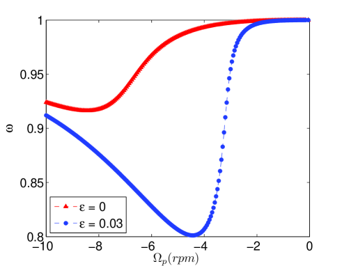
Figure 2: Theoretical amplitude of tilt-over mode angular rotation rate $\omega$ for a spheroid ($\epsilon=0$) and for a slightly deformed triaxial ellipsoid ($\epsilon=0.03$). The other parameters used in this figure are those of Noir_2003 : the rotation rate of the container $\Omega=207\ rpm$ and $a_{1}=0.125\ m$ (such that the Ekman number is $E=3\cdot 10^{-5}$), $\theta=9^{\circ}$, $a_{3}/a_{1}=0.96$ and $\theta_{2}=0^{\circ}$. The spheroidal case corresponds to the plot $\nu=10^{-5}\ m^{2}/s$ in figure 3 of Noir_2003 . Note that even a very small tidal deformation significantly changes the obtained solution.

III Numerical and experimental validation

Our purpose here is to validate and test the range of validity of our analytical solution by comparison with numerical simulations of the full non-linear Navier-Stokes equations in a precessing ellipsoid.

III.1 Numerical resolution

We consider the rotating flow inside a triaxial ellipsoidal container of principal axes $(a_{1},a_{2},a_{3})$, as sketched in figure 1. We work in the precessing frame of reference. Starting from rest, a constant tangential velocity $U\sqrt{1-(x_{3}/a_{3})^{2}}$ is imposed from time $t=0$ all along the outer boundary in each plane of coordinate $x_{3}$ perpendicular to the rotation axis $(O{x_{3}})$, where $U$ is the imposed boundary velocity at the equator. We introduce the timescale $\Omega^{-1}$ by writing the tangential velocity along the deformed outer boundary at the equator $U=\Omega R_{eq}$. We then solve the Navier-Stokes equations with no-slip boundary conditions, taking into account a Coriolis force associated with the precession $\bm{\Omega_{p}}$, i.e. in the frame $(Ox_{1},Ox_{2},Ox_{3})$ of the tidal bulge which is also the precessing frame, we solve:

$$\frac{\partial\mathbf{u}}{\partial t}+\mathbf{u}\cdot\mathbf{\nabla}\mathbf{u}=-\mathbf{\nabla}p+E\bm{\bigtriangleup}\mathbf{u}-2\bm{\Omega_{p}}\times\bm{u},$$ (30)

$$\mathbf{\nabla}\cdot\mathbf{u}=0.$$ (31)

In this work, the range of parameters studied is $E\geq 10^{-3}$ and $\epsilon\leq 0.32$. Once a stationary or periodic state is reached, we determine the rotation rate in the bulk of the fluid, i.e. outside the viscous boundary layer. To do so, we introduce an interior homothetic ellipsoid, in a ratio $\kappa$, and we define the bulk rotation rate $\bm{\omega}$ as the mean value of rotation rate over this homothetic ellipsoid. Following Owen_1989 , we consider a dimensionless viscous layer thickness of $\delta_{\nu}\approx 5\sqrt{E}$ and thus choose for the homothetic ratio $\kappa\approx 1-\delta_{\nu}\approx 1-5\sqrt{E}$. Note that the spheroidal case can be efficiently solved by spectral methods (see e.g. Schmitt_2004 or Wu_2009 ). But for the triaxial ellipsoids we are interested in, there is no simple symmetry. Our computations are thus performed with a finite element method, which allows us to correctly reproduce the geometry and to simply impose the boundary conditions. The solver and the numerical method are described in details in Cebron_2010 .

III.2 Experimental set-up

The experimental set-up has been described in Meunier2008 ; Lagrange2008 for a precessing cylinder and readers should refer to these papers for more details. For this paper, the experiment has been slightly modified in order to study the precession of a spheroid. This allows to validate the flow at small Ekman numbers, which is impossible numerically. Unfortunately, this set-up is limited to a spheroidal geometry ($a_{1}=a_{2}$) and is not able to validate the theory for a tri-axial ellipsoid. Further modifications to the set-up, such as two rollers compressing the spheroid, would be needed to make the equatorial plane elliptical.

The home-made spheroid has been obtained by assembling two half-spheroidal cavities drilled in solid Plexiglas cylinders. The accuracy of the machines ($10$ microns) ensured that the step between the two parts would be smaller than the Ekman layer (of the order of $300$ microns at $E=10^{-5}$). This spheroid of equatorial diameter $17$ cm and aspect ratio $a_{3}/a_{1}=0.85$ is filled with water and mounted on a motor which is itself located on a rotating platform. The angular velocities of the spheroid and the platform are stable within $0.1\%$ and the precessing angle $\theta$ between the two axes was varied from $5^{\circ}$ to $15^{\circ}$ with an accuracy of $0.1^{\circ}$.

Pulsed Yag lasers are used to create a luminous sheet perpendicular to the axis of the rotating platform. A PIV (Particle Image Velocimetry) camera is located on the rotating platform, aligned with the axis of rotation of the spheroid. This allowed to obtain PIV measurements in a plane almost parallel to the equatorial plane $(x_{1},x_{2})$ and located at a distance $x_{3}=5$ cm above it. Since the Yag lasers are not located on the rotating platform, the measurement plane is tilted with an angle $\theta$ with respect to the equatorial plane, which introduces an error of up to 2cm (for $\theta=15^{\circ}$) in the axial location of the velocity vectors. However, the measured velocity components exactly correspond to the $x_{1},x_{2}$ components of the velocity because the camera is aligned with the axis of the spheroid. There is no distortion of the images at the air-Plexiglas interface (because it is a plane) but there are distortions of the images due to the Plexiglas-water spheroidal interface. These deformations are small because the refractive index of the Plexiglas and the water are close. They were calculated analytically and checked experimentally using a grid. They are located mostly at the boundary of the spheroid and they introduce a maximum error of $15\%$ on the radial displacement of the particles. This does not bias the measurements because only the central region of the velocity field was used for the treatment of the data. The PIV images were rotated numerically in order to remove the background rotation of the flow before being treated by a home-made cross-correlation PIV algorithm.

In the frame of reference of the spheroid, the 2D velocity field was found to be a nearly uniform translation flow whose direction and amplitude vary with the precession frequency $\Omega_{p}$. This mean flow is linked to the equatorial component of the angular rotation rate $(\omega_{1},\omega_{2})$ which creates a uniform translation flow $(\alpha_{31}\ x_{3}\ \omega_{2},-\ \alpha_{32}\ x_{3}\ \omega_{1})$ in the plane $x_{3}=5$ cm. This flow corresponds to the last terms found in equations (10) and (11) in the case $a_{1}=a_{2}$. The first terms of these equations correspond to the axial angular rotation $(\omega_{3})$, which in the frame of reference of the spheroid is equal to $\omega_{3}-1$ in dimensionless form and is thus small outside of the resonances. The measurements of the mean velocity and of the mean vorticity thus give in a simple manner the three components of the rotation vector $\bm{\omega}$. Such measurements have been done for the first time in a precessing spheroid, and will be compared to theoretical and numerical results in the following.

III.3 Validation in the spheroidal case

Before dealing with the problem of precessing triaxial ellipsoids, a first step of this work has been to simultaneously check the validity of our numerical tool and the validity of the theoretical development of Busse over an extended range in Ekman number. To do so, we combine numerical and experimental approaches.

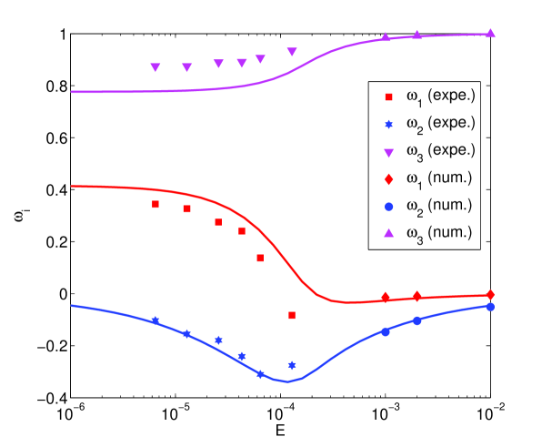
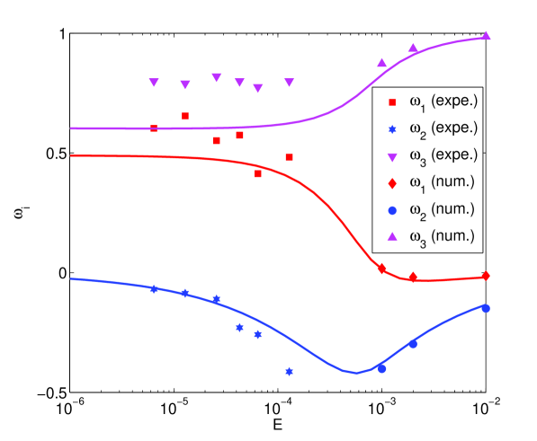
Figure 3: Comparison of the theoretical rotation rate components of Busse’s solution for a spheroid (continuous lines) with experimental PIV measurements and numerical simulations performed over a large range of Ekman numbers for $\Omega_{p}=-0.14$ and $a_{3}/a_{1}=0.85$. (a) For a precession angle of $5^{\circ}$. (b) For a precession angle of $15^{\circ}$.

In figure 3, the theory proposed in Busse is validated over more than three decades of Ekman numbers for two different angles of precession. The interest of the presented results is twofold. Firstly, they validate our numerical model, which will now be used to study triaxial ellipsoids. Secondly, this completes the previous validations of Busse’s theory (e.g. Tilgner_2001, ; Noir_2003, ), in particular for rather large Ekman numbers. Note that, as already noted in Tilgner_2001 , the theoretical analysis requires that the angle between the rotation vector of the container and the rotation vector of the fluid is small since otherwise the Ekman boundary layer analysis is no longer valid. This could explain the differences between the experimental determinations and the theoretical predictions at the highest precessional forcing angle ($\theta=15^{\circ}$). A supplementary confirmation of both the numerical model and Busse’s theory at such Ekman numbers is given in figure 4 (a) where the components of the tilt-over rotation axis are in an excellent agreement for a large range of precession rate. At large precession rates, the inviscid results of Poincare are recovered.

III.4 Numerical simulations of precessing triaxial ellipsoids

A first series of simulations have been performed for $a_{3}/a_{1}=0.86$, $\theta=10^{\circ}$, $\theta_{2}=45^{\circ}$, $E=1/600$, $\epsilon=0.1$ and various precession rates. Results are presented in figure 4 (b). An excellent agreement is found between the numerical simulations and the analytical viscous solution all along the explored range, which demonstrates the validity of our extended viscous theory. Note also that the triaxial Poincaré inviscid flow is recovered far from the resonances. As already noted above, an important feature of the triaxial geometry is the apparition of a second resonance. As already noted in the section II.1, according to the equation (13), the two resonances are in the retrograde regime here because $a_{1},a_{2}>a_{3}$. Note also that as already described in the literature (see e.g. Noir_2003 ), the viscosity naturally smoothes the inviscid resonance peaks but also modifies their position.

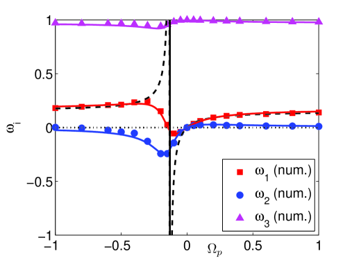
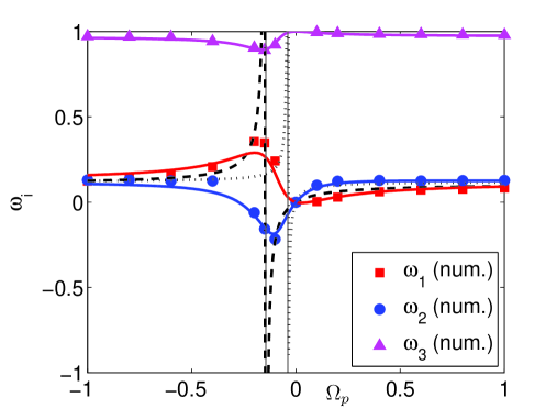
Figure 4: The rotation rate components of the flow in a spheroid, shown in (a), are compared in figure (b) with those in the ellipsoid with the same aspect ratio $a_{3}/a_{1}=0.86$ ($\theta=10^{\circ}$, $\theta_{2}=45^{\circ}$ and $E=1/600$). The theoretical rotation rate components of the inviscid Poincaré solution and of its extension to triaxial ellipsoids are given by the black dashed and dotted lines, assuming that $\omega_{3}=\beta_{12}=\frac{a_{1}^{2}+a_{2}^{2}}{2a_{1}a_{2}}$ (see appendix V). The theoretical rotation rate components of the Busse viscous solution and of its extension to triaxial ellipsoids are represented by the continuous lines. The two inviscid resonances $\gamma_{1}$ and $\gamma_{2}$ are represented by the vertical black lines. (a) In the spheroid, the validity of our numerical model is confirmed over a large range of precession rate by its good agreement with Busse solution. (b) In the ellipsoid with the same aspect ratio but with $\epsilon=0.1$, our analytical solution is in good agreement with the numerical results.

The tilt-over mode is thus well described by our analytical model at relatively large Ekman number and relatively low precession rate and tidal eccentricity. However, two types of instabilities can be expected for more vigorous flows: the tidal or elliptical instability at relatively small Ekman and/or large eccentricity $\epsilon$, and the precession instability at relatively small Ekman and/or large precession rate. Focusing on the tidal instability, we keep the Ekman number above the precession instability threshold, and we increase the eccentricity above the elliptical instability threshold.

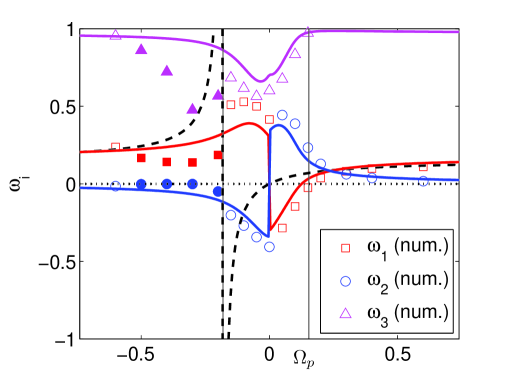
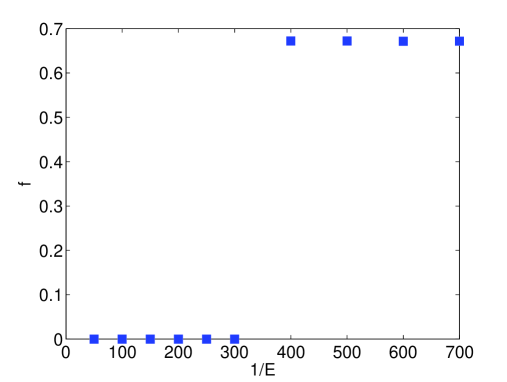
Figure 5: We consider the case $\theta=10^{\circ}$, $a_{3}/a_{1}=0.86$, $\theta_{2}=0$ and $\epsilon=0.317$ (corresponding to $(a_{1}+a_{2})/2=a_{3}$). (a) Evolution of the rotation rate components of the flow with the amplitude of precession for a fixed value of the Ekman number $E=1/600$. Legend is the same as in figure 4 (b). Filled symbols correspond to cases where the flow is oscillatory whereas empty symbols corresponds to a stationary flow. Note that the sign reversal at $\Omega_{p}=0$ is due to the two possible symmetric orientations of the spinover mode of the tidal instability. (b) We now focus on the $\Omega_{p}=-0.4$ case where the flow is oscillatory at $E=1/600$ as shown in (a), and we study the evolution of the pulsation $f$ of the flow with the Ekman number. The flow is stationary for an Ekman number larger than $E=1/300$, and then oscillates at a fixed pulsation $f\approx 0.67$.

The appearance and form of the tidal instability in the presence of a rotating tidal deformation aligned with the rotation axis have been studied elsewhere LeBars09 ; Cebron_2010 . This case corresponds in our notations to the specific configuration $\theta=0$. The most well-known mode is the so called spin-over mode, which appears for low values of tidal bulge rotation. As shown in appendix V, a theoretical stability analysis demonstrates that this mode may grow upon the Poincaré flow. Note that the spin-over mode, which is an unstable mode of the tidal instability, and the tilt-over mode, which is the base flow of precession, are actually identical, hence should both be described by our stationary analytical solution. This is indeed the case, as shown in figure 5 (a) around $\Omega_{p}=0$ where numerical and analytical solutions are in good agreement. Moreover, by comparison with the known results of the elliptical instability in the special case $\theta=0$ (see LeBars09 and Cebron_2010 for details), we expect the elliptical instability to lead to an unstationary mode for $\Omega_{p}$ below the resonance band of the spin-over, and to no elliptical instability for $\Omega_{p}$ above the resonance band of the spin-over. These results are also recovered in figure 5 (a), where oscillatory motions are indeed observed for $\Omega_{p}\in[-0.5;-0.2]$, whereas good agreement is found for $\Omega_{p}>0$ between analytical and numerical results. Finally, a systematic study of the excited mode frequency as a function of the Ekman number for $\Omega_{p}=-0.4$ is shown in figure 5 (b). As expected from the stability analysis presented in appendix V, the transition from a stationary flow to an unstationary one is found below $E\approx 1/300$.

IV Conclusion

This paper presents the first analytical solution and the first numerical simulations of the precessing flow inside a triaxial ellipsoid. The extension of Busse viscous solution to this more complex geometry is shown to provide an accurate description of the stationary flow, which may be destabilized by oscillating modes of the tidal and/or precession instabilities for more vigorous forcing. Clearly, the complete study of instabilities in such a system deserves more work and will be the subject of future studies with increased numerical power and a new experimental set-up. But the study of the stationary flow performed here already highlights the fact that even a very small tidal deformation significantly modifies the resulting flow. This conclusion is directly relevant to the dynamics of planetary cores and atmospheres, where precession and tidal deformation simultaneously take place.

V Appendix: Instability of the inviscid Poincaré flow in a triaxial ellipsoid

The work Naing_2009 have recently studied the stability of a rotating flow with elliptical streamlines in the particular case where the rotation axis executes a constant precessional motion about a perpendicular axis. Using the WKB method, Naing_2009 achieve to quantify both the influence of this particular precession on the elliptical instability, and the influence of the strain on the Coriolis instability for such an unbounded cylindrical base flow. In this appendix, we consider the stability of the inviscid Poincaré flow in triaxial ellipsoids against small inviscid perturbative rotations. The theoretical expression of the growth rate for perturbations that are linear in space variables (i.e. corresponding to the classical spin-over mode) can be readily obtained with the same method as in Gledzer92 , but with the base flow $\mathbf{U}$ obtained in section II.1, using an arbitrary value of $\omega_{3}$. As remind in Kerswell_2002 , the most general perturbation-flow linear in the spatial coordinates is

$$u_{k}-U_{k}=K_{i+1}(t)\ \frac{a_{i}}{a_{i-1}}\ x_{i-1}-K_{i-1}(t)\ \frac{a_{i}}{a_{i+1}}\ x_{i+1}$$ (32)

where the scalar amplitude $K_{i}$ of these small inviscid perturbative rotations can be written $K_{i}=\varepsilon\ k_{i}\ e^{\sigma t}$. The total flow $\mathbf{u}$ have to satisfy the inviscid vorticity equation. Then, $\mathbf{U}$ being solution flow at order $0$, the solution flow at first order in $\epsilon$ is solution of

$$M\ \mathbf{k}=0$$ (33)

where $\mathbf{k}=\left(k_{i}\right)_{i\in(1,2,3)}$ and $M$ is a $3\times 3$ matrix given by

$$M=\left[\begin{array}[]{ccc}A_{12}&-A_{21}&-B_{12}\ \sigma\\ C_{1}&B_{13}\ \sigma&D_{12}\\ -B_{23}\ \sigma&C_{2}&D_{21}\\ \end{array}\right]$$ (37)

where

$$A_{ij}=2\ \Omega_{p,j}\ \frac{a_{3}}{a_{j}}\frac{\gamma_{i}}{\gamma_{j}},$$

$$B_{ij}=\frac{a_{i}^{2}+a_{j}^{2}}{a_{i}\ a_{j}},$$

$$C_{i}=\frac{\gamma_{i}}{a_{3}\ a_{i}},$$

$$D_{ij}=-4\frac{\Omega_{p,i}\ \Omega_{p,3}\ a_{j}^{2}}{\gamma_{i}}.$$

The solution flow at first order is non-trivial if $\det(M)=0$, and the growth rate $\sigma$ is obtained in solving this equation. Actually, the $3^{rd}$ degree equation $\det(M)=0$ writes in the simple form $\sigma^{3}+p\ \sigma=0$, and the growth rate is given by:

$$\sigma=\sqrt{-p}=\sqrt{\frac{A_{12}B_{13}D_{21}+A_{21}B_{23}D_{12}-C_{1}C_{2}B_{12}}{B_{13}B_{23}B_{12}}}$$ (38)

Note that the dimensionless base flow of Gledzer92 is recovered for the particular value $\omega_{3}=\beta_{12}$. It can also be noticed that the extension of the result of Gledzer92 to the particular case of a rotating tidal bulge at $\bm{\Omega_{p}}=(0,0,\Omega_{br})$ given in Cebron_2010 , is recovered:

$$\sigma=\sqrt{-\frac{C_{1}C_{2}}{B_{13}B_{23}}}=\sqrt{-\frac{(a_{1}^{2}-a_{3}^{2}+2a_{1}a_{2}\Omega_{br})(a_{2}^{2}-a_{3}^{2}+2a_{1}a_{2}\Omega_{br})}{(a_{1}^{2}+a_{3}^{2})(a_{2}^{2}+a_{3}^{2})}}.$$ (39)

Note finally that this method gives the theoretical inviscid growth rate, which has then to be corrected by a viscous surfacic damping term $\chi\sqrt{E}$ Kudlick , where $\chi$ is a constant $\chi\sim 2.62$. The threshold is then given explicitly by

$$E_{c}=\frac{1}{\chi^{2}}\frac{A_{12}B_{13}D_{21}+A_{21}B_{23}D_{12}-C_{1}C_{2}B_{12}}{B_{13}B_{23}B_{12}}$$ (40)

For the case presented in figure 5, i.e. $\theta=10^{\circ}$, $a_{3}=(a_{1}+a_{2})/2$, $\theta_{2}=0$ and $\epsilon=0.317$, we predict a critical Ekman number for instability around $E_{c}\approx 1/300$, and for $E=1/600$, we predict an unstable spin-over mode in the range $\Omega_{p}\in[-0.13;0.12]$.

References

- (1) W. Malkus, Lectures on Solar and Planetary Dynamos (Energy sources for planetary dynamos). Cambridge University Press, London, 1993. (ed. MRE Proctor, AD Gilbert).
- (2) A. Tilgner, “Precession driven dynamo,” Phys. Fluids, vol. 17, p. 034104, 2005.
- (3) R. Poincaré, “Sur la précession des corps déformables,” Bull. Astr. 27, vol. 27, pp. 321–356, 1910.
- (4) K. Stewartson and P. Roberts, “On the motion of a liquid in a spheroidal cavity of precessing rigid body,” J. Fluid Mech., vol. 17, pp. 1–20, 1963.
- (5) F. Busse, “Steady fluid flow in a precessing spheroidal shell,” J. Fluid Mech., vol. 33, pp. 739–751, 1968.
- (6) H. Greenspan, The theory of rotating fluids. Cambridge University Press, Cambridge, 1968.
- (7) W. Malkus, “Precession of the earth as the cause of geomagnetism,” Science, vol. 160, pp. 259–264, 1968.
- (8) J. P. Vanyo, P. Wilde, P. Cardin, and P. Olson, “Experiments on precessing flows in the earth’s liquid core,” Geophys. J. Int., vol. 121, pp. 136–142, 1995.
- (9) J. Noir, P. Cardin, D. Jault, and J. P. Masson, “Experimental evidence of nonlinear resonance effects between retrograde precession and the tilt-over mode within a spheroid,” Geophys. J. Int., vol. 154, pp. 407–416, 2003.
- (10) R. Hollerbach and R. R. Kerswell, “Oscillatory internal shear layers in rotating an1d precessing flows,” J. Fluid Mech., vol. 298, pp. 327–339, 1995.
- (11) L. Quartapelle and M. Verri, “On the spectral solutions of the 3-dimensional navier-stokes equations in spherical and cylindrical regions,” Bull. Astr. 27, vol. 90, pp. 1–43, 1995.
- (12) A. Tilgner, “Magnetohydrodynamic flow in precessing spherical shells,” Geophys. J. Int., vol. 379, pp. 303–318, 1999.
- (13) A. Tilgner and F. H. Busse, “Fluid flows in precessing spherical shells,” J. Fluid Mech., vol. 426, pp. 387–396, 2001.
- (14) J. Noir, D. Jault, and C. P., “Numerical study of the motions within a slowly precessing sphere at low ekman number,” J. Fluid Mech., vol. 437, pp. 283–299, 2001.
- (15) M. R. Walker and C. F. Barenghi, “High resolution numerical dynamos in the limit of a thin disk galaxy,” Geophys. Astrophys. Fluid Dyn., vol. 76, pp. 265–281, 1994.
- (16) A. Tilgner, “Non-axisymmetric shear layers in precessing fluid ellipsoidal shells,” J. Fluid Mech, vol. 136, pp. 629–636, 1999.
- (17) S. Lorenzani and A. Tilgner, “Fluid instabilities in precessing spheroidal cavities,” J. Fluid Mech., vol. 447, pp. 111–128, 2001.
- (18) S. Lorenzani and A. Tilgner, “Inertial instabilities of fluid flow in precessing spheroidal shells,” J. Fluid Mech., vol. 492, pp. 363–379, 2003.
- (19) D. Schmitt and D. Jault, “Numerical study of a rotating fluid in a spheroidal container,” J. Comp. Phys., vol. 197, pp. 671–685, 2004.
- (20) C.-C. Wu and P. H. Roberts, “On a dynamo driven by topographic precession,” Geophys. Astrophys. Fluid Dyn., vol. 103, pp. 467–501, 2009.
- (21) R. Kerswell and W. V. R. Malkus, “Tidal instability as the source for Io’s magnetic signature,” Geophys. Res. Lett., vol. 25, pp. 603–606, 1998.
- (22) L. Lacaze, P. Le Gal, and S. Le Dizès, “Elliptical instability in a rotating spheroid,” J. Fluid Mech., vol. 505, pp. 1–22, 2004.
- (23) M. Le Bars, M. Lacaze, S. Le Dizès, P. Le Gal, and M. Rieutord, “Tidal instability in stellar and planetary binary system,” Phys. Earth Planet. Int., vol. 178, pp. 48–55, 2010.
- (24) D. Cébron, M. Le Bars, J. Leontini, P. Maubert, and P. Le Gal, “A systematic numerical study of the tidal instability in a rotating ellipsoid,” Phys. Earth Planet. Int., vol. 182, pp. 119–128, 2010.
- (25) R. Kerswell, “Elliptical instability,” Annu. Rev. Fluid Mech., vol. 34, pp. 83–113, 2002.
- (26) F. A. Waleffe, “On the three-dimensional instability of strained vortices,” Phys. Fluids, vol. 2, pp. 76–80, 1990.
- (27) M. Le Bars, S. Le Dizès, and P. Le Gal, “Coriolis effects on the elliptical instability in cylindrical and spherical rotating containers,” J. Fluid Mech., vol. 585, pp. 323–342, 2007.
- (28) R. Kerswell, “The instability of precessing flow,” Geophys. Astrophys. Fluid Dyn, vol. 72, pp. 107–144, 1993.
- (29) R. Kerswell, “On the internal shear layers spawned by the critical regions in oscillatory ekman boundary layers,” J. Fluid Mech., vol. 298, pp. 311–325, 1995.
- (30) R. Lagrange, P. Meunier, C. Eloy, and F. Nadal, “Instability of a fluid inside a precessing cylinder,” Phys. Fluids, vol. 20, p. 081701, 2008.
- (31) J. Noir, Ecoulement d’un fluide dans une cavité en précession: approches numériques et expérimentales. PhD thesis, Université Joseph-Fourier, Grenoble 1, 2000.
- (32) J. M. Owen and R. H. Rogers, Flow and heat transfer in rotating disc systems (Vol. 1, Rotor-stator systems). Research Studies Press, Taunton, UK & John Wiley, NY, 1989.
- (33) P. Meunier, C. Eloy, R. Lagrange, and F. Nadal, “A rotating fluid cylinder subject to weak precession,” J. Fluid Mech., vol. 599, pp. 405–440, 2008.
- (34) M. M. Naing and Y. Fukumoto, “Local instability of an elliptical flow subjected to a coriolis force,” J. Phys. Soc. Jpn., vol. 78, p. 124401, 2009.
- (35) E. B. Gledzer and V. M. Ponomarev, “Instability of bounded flows with elliptical streamlines,” J. Fluid Mech, vol. 240, pp. 1–30, 1992.
- (36) M. Kudlick, On the transient motions in a contained rotating fluid. PhD thesis, Massachusetts Institute of Technology, 1966.