The KL-UCB Algorithm for Bounded Stochastic Bandits and Beyond

Abstract

This paper presents a finite-time analysis of the KL-UCB algorithm, an online, horizon-free index policy for stochastic bandit problems. We prove two distinct results: first, for arbitrary bounded rewards, the KL-UCB algorithm satisfies a uniformly better regret bound than UCB and its variants; second, in the special case of Bernoulli rewards, it reaches the lower bound of Lai and Robbins. Furthermore, we show that simple adaptations of the KL-UCB algorithm are also optimal for specific classes of (possibly unbounded) rewards, including those generated from exponential families of distributions. A large-scale numerical study comparing KL-UCB with its main competitors (UCB, MOSS, UCB-Tuned, UCB-V, DMED) shows that KL-UCB is remarkably efficient and stable, including for short time horizons. KL-UCB is also the only method that always performs better than the basic UCB policy. Our regret bounds rely on deviations results of independent interest which are stated and proved in the Appendix. As a by-product, we also obtain an improved regret bound for the standard UCB algorithm.

1 Introduction

The multi-armed bandit problem is a simple, archetypal setting of reinforcement learning, where an agent facing a slot machine with several arms tries to maximize her profit by a proper choice of arm draws. In the stochastic bandit problem, the agent sequentially chooses, for $t=1,2,\dots,n$, an arm $A_{t}\in\{1,\dots,K\}$, and receives a reward $X_{t}$ such that, conditionally on the arm choices $A_{1},A_{2},\dots$, the rewards are independent and identically distributed, with expectation $\mu_{A_{1}},\mu_{A_{2}},\dots$. Her policy is the (possibly randomized) decision rule that, to every past observations $(A_{1},X_{1},\dots,A_{t-1},X_{t-1})$, associates her next choice $A_{t}$. The best choice is any arm $a^{*}$ with maximal expected reward $\mu_{a^{*}}$. The performance of her policy can be measured by the regret $R_{n}$, defined as the difference between the rewards she accumulates up to the horizon $t=n$, and the rewards that she would have accumulated during the same period, had she known from the beginning which arm had the highest expected reward.

The agent typically faces an “exploration versus exploitation dilemma” : at time $t$, she can take advantage of the information she has gathered, by choosing the so-far best performing arm, but she has to consider the possibility that the other arms are actually under-rated and she must play sufficiently often all of them. Since the works of Gittins (1979) in the 1970s, this problem raised much interest and several variants, solutions and extensions have been proposed, see Even-Dar et al. (2002) and references therein.

Two families of bandit settings can be distinguished: in the first family, the distribution of $X_{t}$ given $A_{t}=a$ is assumed to belong to a family $\{p_{\theta},\theta\in\Theta_{a}\}$ of probability distributions. In a particular parametric framework, Lai and Robbins (1985) proved a lower-bound on the performance of any policy, and determined optimal policies. This framework was extended to multi-parameter models by Burnetas and Katehakis (1997) who showed that the number of draws up to time $n$, $N_{a}(n)$, of any sub-optimal arm $a$ is lower-bounded by

$$N_{a}(n)\geq\left(\frac{1}{\inf_{\theta\in\Theta_{a}:E[p_{\theta}]>\mu_{a^{*}}}KL\left(p_{\theta_{a}},p_{\theta}\right)}+o(1)\right)\;\log(n),$$ (1)

where $KL$ denotes the Kullback-Leibler divergence and $E(p_{\theta})$ is the expectation under $p_{\theta}$; hence, the regret is lower-bounded as follows:

$$\liminf_{n\to\infty}\frac{\mathbb{E}[R_{n}]}{\log(n)}\geq\sum_{a:\mu_{a}<\mu_{a^{*}}}\frac{\mu_{a^{*}}-\mu_{a}}{\inf_{\theta\in\Theta_{a}:E[p_{\theta}]>\mu_{a^{*}}}KL\left(p_{\theta_{a}},p_{\theta}\right)}\;.$$ (2)

Recently, Honda and Takemura (2010) proposed an algorithm called Deterministic Minimum Empirical Divergence (DMED) which they proved to be first order optimal. This algorithm, which maintains a list of arms that are close enough to the best one (and which thus must be played), is inspired by large deviations ideas and relies on the availability of the rate function associated to the reward distribution.

In the second family of bandit problems, the rewards are only assumed to be bounded (say, between $0$ and $1$), and policies rely directly on the estimates of the expected rewards for each arm. The KL-UCB algorithm considered in this paper is primarily meant to address this second, non-parametric, setting. We will nonetheless show that KL-UCB also matches the lower bound of Burnetas and Katehakis (1997) in the binary case and that it can be extended to a larger class of parametric bandit problems.

Among all the bandit policies that have been proposed, a particular family has raised a strong interest, after Gittins (1979) proved that (in the Bayesian setting he considered) optimal policies could be chosen in the following very special form: compute for each arm a dynamic allocation index (which only depends on the draws of this arm), and simply choose an arm with maximal index. These policies not only compute an estimate of the expected rewards, but rather an upper-confidence bound (UCB), and the agent’s choice is an arm with highest UCB. This approach is sometimes called “optimistic”, as the agent acts as if, at each instant, the expected rewards were equal to the highest possible values that are compatible with her past observations. Auer et al. (2002), following Agrawal (1995), proposed and analyzed two variants, UCB1 (usually called simply UCB in latter works) and UCB2, for which they provided regret bounds. UCB is an online, horizon-free procedure for which (Auer et al., 2002) proves that there exists a constant $C$ such that

$$\mathbb{E}[R_{n}]\leq\sum_{a:\mu_{a}<\mu_{a^{*}}}\frac{8\log(n)}{\left(\mu_{a^{*}}-\mu_{a}\right)}+C\;.$$ (3)

The UCB2 variant relies on a parameter $\alpha$ that needs to be tuned, depending in particular on the horizon, and satisfies the tighter regret bound

$$\mathbb{E}[R_{n}]\leq\sum_{a:\mu_{a}<\mu_{a^{*}}}\frac{(1+\epsilon(\alpha))\log(n)}{2\left(\mu_{a^{*}}-\mu_{a}\right)}+C(\alpha)\;,$$

where $\epsilon(\alpha)>0$ is a constant that can get arbitrary small when $\alpha$ is small, at the expense of an increased value of the constant $C(\alpha)$. The constant $1/2$ in front of the factor $\log(n)/\left(\mu_{a^{*}}-\mu_{a}\right)$ cannot be improved. We show in Proposition 3.4, as a by-product of our analysis, that a correctly tuned UCB algorithm satisfies a similar bound. However, Auer et al. (2002) found in numerical experiments that UCB and UCB2 were outperformed by a third heuristic variant called UCB-Tuned, which includes estimates of the variance, but no theoretical guarantee was given. In a latter work, Audibert et al. (2009) proposed a related policy, called UCB-V, which uses an empirical version of the Bernstein bound to obtain refined upper confidence bounds. Recently, Audibert and Bubeck (2010) introduced an improved UCB algorithm, termed MOSS, which achieves the distribution-free optimal rate.

In this contribution, we first consider the stochastic, non-parametric, bounded bandit problem. We consider an online index policy, called KL-UCB (for Kullback-Leibler UCB), that requires no problem- or horizon-dependent tuning. This algorithm was recently advocated by Filippi (2010), together with a similar procedure for Markov Decision Processes (Filippi et al., 2010), and we learnt since our initial submission that an analysis of the Bernoulli case can also be found in Maillard et al. (2011), together with other results. We prove in Theorem 3.1 below that the regret of KL-UCB satisfies

$$\limsup_{n\to\infty}\frac{\mathbb{E}[R_{n}]}{\log(n)}\leq\sum_{a:\mu_{a}<\mu_{a^{*}}}\frac{\mu_{a^{*}}-\mu_{a}}{d(\mu_{a},\mu_{a^{*}})}\;,$$

where $d(p,q)=p\log(p/q)+(1-p)\log((1-p/(1-q))$ denotes the Kullback-Leibler divergence between Bernoulli distributions of parameters $p$ and $q$, respectively. This comes as a consequence of Theorem 3.2, a non-asymptotic upper-bound on the number of draws of a sub-optimal arm $a$: for all $\epsilon>0$ there exist $C_{1},C_{2}(\epsilon)$ and $\beta(\epsilon)$ such that

$$\mathbb{E}[N_{n}(a)]\leq\frac{\log(n)}{d(\mu_{a},\mu_{a^{*}})}(1+\epsilon)+C_{1}\log(\log(n))+\frac{C_{2}(\epsilon)}{n^{\beta(\epsilon)}}\;.$$

We insist on the fact that, despite the presence of divergence $d$, this bound is not specific to the Bernoulli case and applies to all reward distributions bounded in $[0,1]$ (and thus, by rescaling, to all bounded reward distributions). By Pinsker’s inequality, $d(\mu_{a},\mu_{a^{*}})>2(\mu_{a}-\mu_{a^{*}})^{2}$, and thus KL-UCB has strictly better theoretical guarantees than UCB, while it has the same range of application. The improvement appears to be significant in simulations. Moreover, KL-UCB is the first index policy that reaches the lower-bound of Lai and Robbins (1985) for binary rewards; it does also achieve lower regret than UCB-V in that case. Hence, KL-UCB is both a general-purpose procedure for bounded bandits, and an optimal solution for the binary case.

Furthermore, it is easy to adapt KL-UCB to particular (possibly non-bounded) bandit settings, when the distribution of reward is known to belong to some family of probability laws. By simply changing the definition of the divergence $d$, optimal algorithms may be built in a great variety of situations.

The proofs we give for these results are short and elementary. They rely on deviation results for bounded variables that are of independent interest : Lemma A.1 shows that Bernoulli variable are, in a sense, the “least concentrated” bounded variables with a given expectation (as is well-known for variance), and Theorem A.3 shows an efficient way to build confidence intervals for sums of bounded variables with an unknown number of summands.

In practice, numerical experiments confirm the significant advantage of KL-UCB over existing procedures; not only does this method outperform UCB, MOSS, UCB-V and even UCB-tuned in various scenarios, but it also compares well to DMED in the Bernoulli case, especially for small or moderate horizons.

The paper is organized as follows: in Section 2, we introduce some notation and present the KL-UCB algorithm. Section 3 contains the main results of the paper, namely the regret bound for KL-UCB and the optimality in the Bernoulli case. In Section 4, we show how to adapt the KL-UCB algorithm to address general families of reward distributions, and we provide finite-time regret bounds showing asymptotic optimality. Section 5 reports the results of extensive numerical experiments, showing the practical superiority of KL-UCB. Section 6 is devoted to an elementary proof of the main theorem. Finally, the Appendix gathers some deviation results that are useful in the proofs of our regret bounds, but which are also of independent interest.

2 The KL-UCB Algorithm

We consider the following bandit problem: the set of actions is $\{1,\dots,K\}$, where $K$ denotes a finite integer. For each $a\in\{1,\dots,K\}$, the rewards $(X_{a,t})_{t\geq 1}$ are independent and bounded in $\Theta=[0,1]$ with common expectation $\mu_{a}$. The sequences $(X_{a,\cdot})_{a}$ are independent. At each time step $t=1,2,\dots$, the agent chooses an action $A_{t}$ according to his past observations (possibly using some independent randomization) and gets the reward $X_{t}=X_{A_{t},N_{A_{t}}(t)}$, where $N_{a}(t)=\sum_{s=1}^{t}\mathbbm{1}\{A_{s}=a\}$ denotes the number of times action $a$ was chosen up to time $t$. The sum of rewards she has obtained when choosing action $a$ is denoted by $S_{a}(t)=\sum_{s\leq t}\mathbbm{1}\{A_{s}=a\}X_{s}=\sum_{s=1}^{N_{a}(t)}X_{a,s}$. For $(p,q)\in\Theta^{2}$ denote the Bernoulli Kullback-Leibler divergence by

$$d(p,q)=p\log\frac{p}{q}+(1-p)\log\frac{1-p}{1-q}\;,$$

with, by convention, $0\log 0=0\log 0/0=0$ and $x\log x/0=+\infty$ for $x>0$.

Algorithm 1 KL-UCB

0:  $n$ (horizon), $K$ (number of arms), REWARD (reward function, bounded in $[0,1]$)

1:  for $t=1$ to $K$ do

2:     $N[t]\leftarrow 1$

3:     $S[t]\leftarrow\hbox{REWARD}(\hbox{arm}=t)$

4:  end for

5:  for $t=K+1$ to $n$ do

6:     $a\leftarrow\operatorname*{arg\,max}_{1\leq a\leq K}\max\left\{q\in\Theta:N[a]\,d\left(\frac{S[a]}{N[a]},q\right)\leq\log(t)+c\log(\log(t))\right\}$

7:     $r\leftarrow\hbox{REWARD}(\hbox{arm}=a)$

8:     $N[a]\leftarrow N[a]+1$

9:     $S[a]\leftarrow S[a]+r$

10:  end for

Algorithm 1 provides the pseudo-code for KL-UCB. On line 6, $c$ is a parameter that, in the regret bound stated below in Theorem 3.1 is chosen equal to $3$; in practice, however, we recommend to take $c=0$ for optimal performance. For each arm $a$ the upper-confidence bound

$$\max\left\{q\in\Theta:N[a]\,d\left(\frac{S[a]}{N[a]},q\right)\leq\log(t)+c\log(\log(t))\right\}$$

can be efficiently computed using Newton iterations, as for any $p\in[0,1]$ the function $q\mapsto d(p,q)$ is strictly convex and increasing on the interval $[p,1]$. In case of ties between severals arms, any maximizer can be chosen (for instance, at random). The KL-UCB elaborates on ideas suggested in Sections 3 and 4 of Lai and Robbins (1985).

3 Regret bounds and optimality

We first state the main result of this paper. It is a direct consequence of the non-asymptotic bound in Theorem 3.2 stated below.

Theorem 3.1.

Consider a bandit problem with $K$ arms and independent rewards bounded in $[0,1]$, and denote by $a^{*}$ an optimal arm. Choosing $c=3$, the regret of the KL-UCB algorithm satisfies:

$$\limsup_{n\to\infty}\frac{\mathbb{E}[R_{n}]}{\log(n)}\leq\sum_{a:\mu_{a}<\mu_{a^{*}}}\frac{\mu_{a^{*}}-\mu_{a}}{d(\mu_{a},\mu_{a^{*}})}\;.$$

Theorem 3.2.

Consider a bandit problem with $K$ arms and independent rewards bounded in $[0,1]$. Let $\epsilon>0$, and take $c=3$ in Algorithm 1. Let $a^{*}$ denote an arm with maximal expected reward $\mu_{a^{*}}$, and let $a$ be an arm such that $\mu_{a}<\mu_{a^{*}}$. For any positive integer $n$, the number of times algorithm KL-UCB chooses arm $a$ is upper-bounded by

$$\mathbb{E}[N_{n}(a)]\leq\frac{\log(n)}{d(\mu_{a},\mu_{a^{*}})}(1+\epsilon)+C_{1}\log(\log(n))+\frac{C_{2}(\epsilon)}{n^{\beta(\epsilon)}}\;,$$

where $C_{1}$ denotes a positive constant and where $C_{2}(\epsilon)$ and $\beta(\epsilon)$ denote positive functions of $\epsilon$. Hence,

$$\limsup_{n\to\infty}\frac{\mathbb{E}[N_{n}(a)]}{\log(n)}\leq\frac{1}{d(\mu_{a},\mu_{a^{*}})}\;.$$

Corollary 3.3.

If the reward distributions are Bernoulli, the KL-UCB algorithm is asymptotically optimal, in the sense that the regret of KL-UCB matches the lower-bound proved by Lai and Robbins (1985) and generalized by Burnetas and Katehakis (1997):

$$N_{n}(a)\geq\left(\frac{1}{d(\mu_{a},\mu_{a^{*}})}+o(1)\right)\log(n)$$

with a probability tending to $1$.

The KL-UCB algorithm thus appears to be (asymptotically) optimal for Bernoulli rewards. However, Lemma A.1 shows that the Chernoff bounds obtained for Bernoulli variables actually apply to any variable with range $[0,1]$. This is why KL-UCB is not only efficient in the binary case, but also for general bounded rewards.

As a by-product, we obtain an improved upper-bound for the regret of the UCB algorithm:

Proposition 3.4.

Consider the UCB algorithm tuned as follows: at step $t>K$, the arm that maximizes the upper-bound $S[a]/N[a]+\sqrt{(\log(t)+c\log\log(t))/(2N[a])}$ is chosen. Then, for the choice $c=3$, the number of draws of a sub-optimal arm $a$ is upper-bounded as:

$$\mathbb{E}[N_{n}(a)]\leq\frac{\log(n)}{2(\mu_{a}-\mu_{a^{*}})^{2}}(1+\epsilon)+C_{1}\log(\log(n))+\frac{C_{2}(\epsilon)}{n^{\beta(\epsilon)}}\;.$$ (4)

This bound is “optimal”, in the sense that the constant $1/2$ in the logarithmic term cannot be improved. The proof of this proposition just mimics that of Section 6 (which concerns KL-UCB), using the quadratic divergence $d(p,q):=2(p-q)^{2}$ instead of the Kullback-Leibler divergence; it is thus omitted. In contrast, Pinsker’s inequality $d(\mu_{a},\mu_{a^{*}})\geq 2(\mu_{a}-\mu_{a^{*}})^{2}$ shows that KL-UCB dominates UCB, and we will see in the simulation study that the difference is significant, even for smaller values of the horizon.

Remark 3.5.

At line $6$, Algorithm 1 computes for each arm $a\in\{1,\dots,K\}$ the upper-confidence bound

$$\max\left\{q\in\Theta:N[a]\,d\left(\frac{S[a]}{N[a]},q\right)\leq\log(t)+c\log(\log(t))\right\}\;.$$

The level of this confidence bound is parameterized by the exploration function $\log(t)+c\log(\log(t))$, and the results of Theorems 3.1 and 3.2 are true as soon as $c\geq 3$. However, similar results can be proved with an exploration function equal to $(1+\epsilon)\log(t)$ (instead of $\log(t)+c\log(\log(t))$) for every $\epsilon>0$; this is no surprise, as $(1+\epsilon)\log(t)\geq\log(t)+c\log(\log(t))$ when $t$ is large enough. But “large enough”, in that case, can be quite large : for $\epsilon=0.1$, this holds true only for $t>2.10^{51}$. This is why, in practice (and for the simulations presented in Section 5), we rather suggest to choose $c=0$.

4 KL-UCB for parametric families of reward distributions

The KL-UCB algorithm makes no assumption on the distribution of the rewards, except that they are bounded. Actually, the definition of the divergence function $d$ in KL-UCB is dictated by the rate function of the Large Deviations Principle satisfied by Bernoulli random variables: the proof of Theorem A.3 relies on the control of the Fenchel-Legendre transform of the Bernoulli distribution. Thanks to Lemma A.1, this choice also makes sense for all bounded variables.

But the method presented here is not limited to the Bernoulli case: KL-UCB can very easily be adapted to other settings by choosing an appropriate divergence function $d$. As an illustration, we will assume in this section that, for each arm $a$, the distribution of rewards belongs to a canonical exponential family, i.e., that its density with respect to some reference measure can be written as $p_{\theta_{a}}(x)$ for some real parameter $\theta_{a}$, with

$$p_{\theta}(x)=\exp\left(x\theta-b(\theta)+c(x)\right)\;,$$ (5)

where $\theta$ is a real parameter, $c$ is a real function and the $\log$-partition function $b(\cdot)$ is assumed to be twice differentiable. This family contains for instance the Exponential, Poisson, Gaussian (with fixed variance), Gamma (with fixed shape parameter) distributions (as well as, of course, the Bernoulli distribution). For a random variable $X$ with density defined in $\eqref{eq:densiteModeleExpo}$, it is easily checked that $\mu(\theta)\triangleq\mathbb{E}_{\theta}[X]=\dot{b}(\theta)$; moreover, as $\ddot{b}(\theta)=\mathbb{V}ar(X)>0$, the function $\theta\mapsto\mu(\theta)$ is one-to-one. Theorem A.5 (in the Appendix) states that the probability of under-estimating the performance of the best arm can be upper-bounded just as in the Bernoulli case by replacing the divergence $d(\cdot,\cdot)$ in line 6 of the KL-UCB algorithm by

$$d(x,\mu(\theta))=\sup_{\lambda}\left\{\lambda x-\log\mathbb{E}_{\theta}\left[\exp(\lambda X)\right]\right\}\;.$$

For example, in the case of exponential rewards, one should choose $d(x,y)=x/y-1-\log(x/y)$. Or, for Poisson rewards, the right choice is $d(x,y)=y-x+x\log(x/y)$. Then, all the results stated above apply (as the proofs do not involve the particular form of the function $d$), and in particular :

$$\limsup_{n\to\infty}\frac{\mathbb{E}[R_{n}]}{\log(n)}\leq\sum_{a:\mu_{a}<\mu_{a^{*}}}\frac{\mu_{a^{*}}-\mu_{a}}{d(\mu_{a},\mu_{a^{*}})}\;.$$

In order to prove that, for those families of rewards, this version of the KL-UCB algorithm matches the bound of Lai and Robbins (1985) , it remains only to show that $d(x,y)=KL(p_{\mu^{-1}(x)},p_{\mu^{-1}(y)})$. This is the object of Lemma 4.1. Generalizations to other families of reward distributions (possibly different from arm to arm) are conceivable, but require more technical, topological discussions, as in Burnetas and Katehakis (1997) and Honda and Takemura (2010).

To conclude, observe that it is not required to work with the divergence function $d$ corresponding exactly to the family of reward distributions: using an upper-bound instead often leads to more simple and versatile policies at the price of only a slight loss in performance. This is illustrated in the third scenario of the simulation study presented in Section 5, but also by Theorems 3.1 and 3.2 for bounded variables.

Lemma 4.1.

Let $(\beta,\theta)$ be two real numbers, let $p_{\beta}$ and $p_{\theta}$ be two probability densities of the canonical exponential family defined in (5), and let $X$ have density $p_{\theta}$. Then Kullback-Leibler divergence $KL(p_{\beta},p_{\theta})$ is equal to $d(\mu(\beta),\mu(\theta))$. More precisely,

$$KL(p_{\beta},p_{\theta})=d(\mu(\beta),\mu(\theta))=\mu(\beta)\left(\beta-\theta\right)-b(\beta)+b(\theta)\;.$$

Proof 4.2.

First, it holds that

$$KL(p_{\beta},p_{\theta}) =\int\exp\left(x\beta-b(\beta)+c(x)\right)\left\{x\left(\beta-\theta\right)-b(\beta)+b(\theta)\right\}dx$$

$$=\mu(\beta)\left(\beta-\theta\right)-b(\beta)+b(\theta)\;.$$

Then, observe that $\mathbb{E}\left[\exp(\lambda X)\right]=\int\exp\left(x(\beta+\lambda)-b(\beta)+c(x)\right)dx=\exp(b(\beta+\lambda)-b(\beta))\;.$ Thus, for every $x$ the maximum of the (smooth, concave) function

$$\lambda\mapsto\lambda x-\log\mathbb{E}\left[\exp(\lambda X)\right]=\lambda x-b(\theta+\lambda)+b(\theta)$$

is reached for $\lambda=\lambda^{*}$ such that $x=\dot{b}(\theta+\lambda^{*})=\mu(\theta+\lambda^{*})$. Thus, if $x=\mu(\beta)$, the fact that $\mu$ is one-to-one implies that $\theta+\lambda^{*}=\beta$ and thus that:

$$d(\mu(\beta),\mu(\theta))=\left(\beta-\theta\right)\mu(\beta)-b(\beta)+b(\theta)\;.$$

5 Numerical experiments and comparisons of the policies

Simulations studies require particular attention in the case of bandit algorithms. As pointed out by Audibert et al. (2009), for a fixed horizon $n$ the distribution of the regret is very poorly concentrated around its expectation. This can be explained as follows: most of the time, the estimates of all arms remain correctly ordered for almost all instants $t=1,\dots,n$ and the regret is of order $\log(n)$. But sometimes, at the beginning, the best arm is under-estimated while one of the sub-optimal arms is over-estimated, so that the agent keeps playing the latter; and as she neglects the best arm, she has hardly an occasion to realize her mistake, and the error perpetuates for a very long time. This happens with a small, but not negligible probability, because the regret is very important (of order $n$) on these occasions. Bandit algorithms are typically designed to control the probability of such adverse events but usually at a rate which only decays slightly faster than $1/n$, which results in very skewed regret distributions with slowly vanishing upper tails.

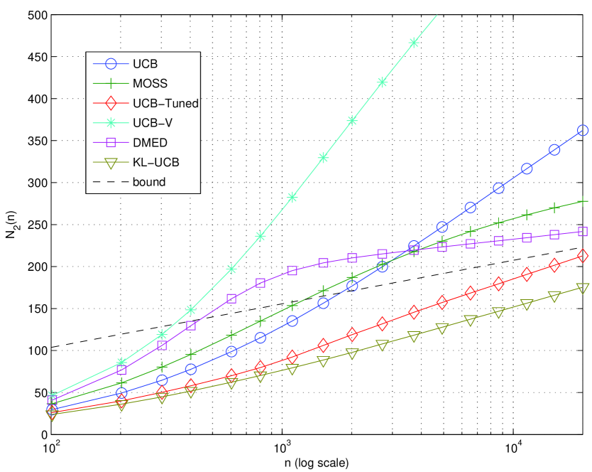
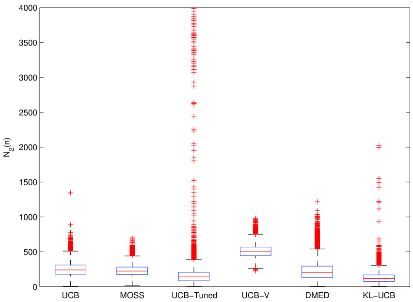
Figure 1: Performance of the various algorithms in the simple two arms, scenario. Left, mean number of draws of the suboptimal arm as a function of time; right, box-plots showing the distributions of the number of draws of the suboptimal arm at time $n=5,000$. Results based on $50,000$ independent runs.

5.1 Scenario 1: two arms

We first consider the basic two arm scenario with Bernoulli rewards of expectations $\mu_{1}=0.9$ and $\mu_{2}=0.8$, respectively. The left panel of Figure 1 shows the average number of draws of the suboptimal arm as a function of time (on a logarithmic scale) for KL-UCB compared to five benchmark algorithms (UCB, MOSS, UCB-Tuned, UCB-V and DMED). The right panel of Figure 1 shows the empirical distributions of suboptimal draws, represented as box-and-whiskers plots, at a particular time ($t=5,000$) for all six algorithms. These plot are obtained from $N=50,000$ independent runs of the algorithms and the right panel of Figure 1 clearly highlight the tail effect mentioned above. On this very simple example, we observed that results obtained from $N=1,000$ or less simulations were not reliable, typically resulting in a significant over-estimation of the performance of “risky” algorithms, in particular of UCB-Tuned. More generally, results obtained in configurations where $N$ is much smaller than $n$ are likely to be unreliable. For this reason, we limit our investigations to a final instant of $n=20,000$. Note however that the average number of suboptimal draws of most algorithms at $n=20,000$ is only of the order of $300$, showing that there is no point in considering larger horizons for such a simple problem.

MOSS, UCB-Tuned and UCB-V are run exactly as described by Audibert and Bubeck (2010), Auer et al. (2002) and Audibert et al. (2009), respectively. For UCB, we use an upper confidence bound $S[a]/N[a]+\sqrt{\log(t)/(2N[a])}$, as in Proposition 3.4, again with $c=0$. Note that in our two arm scenario, $\{2(\mu_{1}-\mu_{2})^{2}\}^{-1}=50$ while $d^{-1}(\mu_{2},\mu_{1})=22.5$. Hence, the performance of DMED and KL-UCB should be about two times better than that of UCB. The left panel of Figure 1 does show the expected behavior but with a difference of lesser magnitude. Indeed, one can observe that the bound $d^{-1}(\mu_{2},\mu_{1})\log(n)$ (shown in dashed line) is quite pessimistic for the values of the horizon $n$ considered here as the actual performance of KL-UCB is significantly below the bound. For DMED, we follow Honda and Takemura (2010) but using

$$N[a]\,d\left(\frac{S[a]}{N[a]},\max_{b}\frac{S[b]}{N[b]}\right)<\log t$$ (6)

as the criterion to decide whether arm $a$ should be included in the list of arms to be played. This criterion is clearly related to the decision rule used by KL-UCB when $c=0$ (see line 6 of Algorithm 1) except for the fact that in KL-UCB the estimate $S[a]/N[a]$ is not compared to that of the current best arm $\max_{b}S[b]/N[b]$ but to the corresponding upper confidence bound. As a consequence, any arm that is not included in the list of arms to be played by DMED would not be played by KL-UCB either (assuming that both algorithms share a common history). As one can observe on the left panel of Figure 1, this results in a degraded performance for DMED. We also observed this effect on UCB, for instance, and it seems that index algorithms are generally preferable to their “arm elimination” variant.

The original proposal of Honda and Takemura (2010) consists in using in the exploration function a factor $\log(t/N[a])$ instead of $\log(t)$, as in the MOSS algorithm. As will be seen below on Figure 2, this variant (which we refer to as DMED+) indeed outperforms DMED. But our previous conjecture appears to hold also in this case as the heuristic variant of KL-UCB (termed KL-UCB+) in which $\log(t)$ in line 6 of Algorithm 1 is replaced by $\log(t/N[a])$ remains preferable to DMED+.

As final comments on Figure 1, first note that UCB-Tuned performs as expected —though slightly worse than KL-UCB— but is a very risky algorithm: the right panel of Figure 1 casts some doubts on the fact that the tails of $N_{a}(n)$ are indeed controlled uniformly in $n$ for UCB-Tuned. Second, the performance of UCB-V is somewhat disappointing. Indeed, the upper-confidence bounds of UCB-V differ from those of UCB-Tuned simply by the non-asymptotic correction term $3\log(t)/N[a]$ required by Bennett’s and Bernstein’s inequalities (Audibert et al., 2009). This correction term appears to have a significant impact on moderate time horizons: for a sub-optimal arm $a$, the number of draws $N[a]$ does not grow faster than the $\log(t)$ exploration function, and $\log(t)/N[a]$ does not vanish.

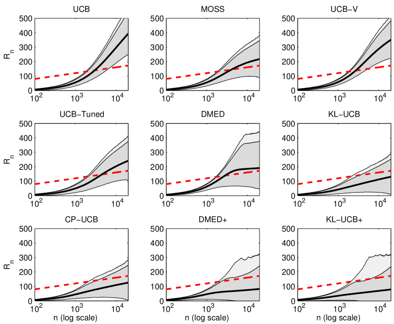
Figure 2: Regret of the various algorithms as a function of time (on a log scale) in the ten arm scenario. On each graph, the red dashed line shows the lower bound, the solid bold curve corresponds to the mean regret while the dark and light shaded regions show respectively the central 99% region and the upper 0.05% quantile, respectively.

5.2 Scenario 2: low rewards

In Figure 2 we consider a significantly more difficult scenario, again with Bernoulli rewards, inspired by a situation (frequent in applications like marketing or Internet advertising) where the mean reward of each arm is very low. In this scenario, there are ten arms: the optimal arm has expected reward 0.1, and the nine suboptimal arms consist of three different groups of three (stochastically) identical arms each with expected rewards 0.05, 0.02 and 0.01, respectively. We again used $N=50,000$ simulations to obtain the regret plots of Figure 2. These plots show, for each algorithm, the average cumulated regret together with quantiles of the cumulated regret distribution as a function of time (again on a logarithmic scale).

In this scenario, the difference is more pronounced between UCB and KL-UCB. The performance gain of UCB-Tuned is also much less significant. KL-UCB and DMED reach a performance that is on par with the lower bound of Burnetas and Katehakis (1997) in (2), although the performance of KL-UCB is here again significantly better. Using KL-UCB+ and DMED+ results in significant mean improvements, although there are hints that those algorithms might indeed be too risky with occasional very large deviations from the mean regret curve.

The final algorithm included in this roundup, called CP-UCB, is in some sense a further adaptation of KL-UCB to the specific case of Bernoulli rewards. For $n\in\mathbb{N}$ and $p\in[0,1]$, denote by $P_{n,p}$ the binomial distribution with parameters $n$ and $p$. For a random variable $X$ with distribution $P_{n,p}$, the Clopper-Pearson (see Clopper and Pearson (1934)) or “exact” upper-confidence bound of risk $\alpha\in]0,1[$ for $p$ is

$$u^{CP}(X,n,\alpha)=\max\left\{q\in[0,1]:P_{n,q}([0,X])\geq\alpha\right\}\;.$$

It is easily verified that $P_{n,p}\left(\mu\leq u^{CP}(X)\right)\geq 1-\alpha$, and that $u^{CP}(X)$ is the smallest quantity satisfying this property: $u^{CP}(X)\leq\tilde{u}(X)$ for any other upper-confidence bound $\tilde{u}(X)$ of risk at most $\alpha$.

The Clopper-Pearson Upper-Confidence Bound algorithm (CP-UCB) differs from KL-UCB only in the way the upper-confidence bound on the performance of each arm is computed, replacing line 6 of Algorithm 1 by

$$a\leftarrow\operatorname*{arg\,max}_{1\leq a\leq K}\;u^{CP}\left(S[a],N[a],\frac{1}{t\log(t)^{c}}\right)\;.$$

As the Clopper-Wilson confidence intervals are always sharper than the Kullback-Leibler intervals, one can very easily adapt the proof of Section 6 to show that the regret bounds proved for the KL-UCB algorithm also hold for CP-UCB in the case of Bernoulli rewards. However, the improvement over KL-UCB is very limited (often, the two algorithms actually take exactly the same decisions). In terms of results, one can observe on Figure 2 that CP-UCB only achieves a performance that is marginally better than that of KL-UCB. Besides, there is no guarantee that the CP-UCB algorithm is also efficient on arbitrary bounded distributions.

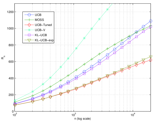
Figure 3: Regret of the various algorithms as a function of time in the bounded exponential scenario.

5.3 Scenario 3: bounded exponential rewards

In the third example, there are $5$ arms: the rewards are exponential variables, with parameters $1/5$, $1/4$, $1/3$, $1/2$ and $1$ respectively, truncated at $x_{\max}=10$ (thus, they are bounded in $[0,10]$). The interest of this scenario is twofold: first, it shows the performance of KL-UCB for non-binary, non-discrete, non $[0,1]$-valued rewards. Second, it illustrates that, as explained in Section 4, specific variants of the KL-UCB algorithm can reach an even better performance.

In this scenario, UCB and MOSS, but also KL-UCB are clearly sub-optimal. UCB-Tuned and UCB-V, by taking into account the variance of the reward distributions (much smaller than the variance of a $\{0,10\}$-valued distribution with the same expectation), were expected to perform significantly better. For the reasons mentionned above this is not the case for UCB-V on a time horizon $n=20,000$. Yet, UCB-Tuned is spectacularly more efficient, and is only caught up by KL-UCB-exp, the variant of KL-UCB designed for exponential rewards. Actually, the KL-UCB-exp algorithm ignores the fact that the rewards are truncated, and uses the divergence $d(x,y)=x/y-1-\log(x/y)$ prescribed for genuine exponential distributions. One can easily show that this choice leads to slightly too large upper confidence bounds. Yet, the performance is still excellent, stable, and the algorithm is particularly simple.

6 Proof of Theorem 3.2

Consider a positive integer $n$, a small $\epsilon>0$, an optimal arm $a^{*}$ and a sub-optimal arm $a$ such that $\mu_{a}<\mu_{a^{*}}$. Without loss of generality, we will assume that $a^{*}=1$. For any arm $b$, the past average performance of arm $b$ is denoted by $\hat{\mu}_{b}(t)=S_{b}(t)/N_{b}(t)$; by convenience, for every positive integer $s$ we will also denote $\hat{\mu}_{b,s}=\left(X_{b,1}+\dots+X_{b,s}\right)/s$, so that $\hat{\mu}_{t}(b)=\hat{\mu}_{b,N_{b}(t)}$. KL-UCB relies on the following upper-confidence bound for $\mu_{b}$:

$$u_{b}(t)=\max\left\{q>\hat{\mu}_{b}(t):N_{b}(t)\,d\left(\hat{\mu}_{b}(t),q\right)\leq\log(t)+3\log(\log(t))\right\}\;.$$

For $x,y\in[0,1]$, define $d^{+}(x,y)=d(x,y)\mathbbm{1}_{x<y}$. The expectation of $N_{n}(a)$ is upper-bounded by using the following decomposition:

$$\mathbb{E}[N_{n}(a)] =\mathbb{E}\left[\sum_{t=1}^{n}\mathbbm{1}\{A_{t}=a\}\right]\leq\mathbb{E}\left[\sum_{t=1}^{n}\mathbbm{1}\{\mu_{1}>u_{1}(t)\}\right]+\mathbb{E}\left[\sum_{t=1}^{n}\mathbbm{1}\{A_{t}=a,\mu_{1}\leq u_{1}(t)\}\right]$$

$$\leq\sum_{t=1}^{n}\mathbb{P}\left(\mu_{1}>u_{1}(t)\right)+\mathbb{E}\left[\sum_{s=1}^{n}\mathbbm{1}\{sd^{+}(\hat{\mu}_{a,s},\mu_{1})<\log(n)+3\log(\log(n))\}\right]\;,$$

where the last inequality is a consequence of Lemma 6.1. The first summand is upper-bounded as follows: by Theorem A.3 (proved in the Appendix),

$$P(\mu_{1}>u_{1}(t)) \leq e\left\lceil\log(t)\left(\log(t)+3\log(\log(t))\right)\right\rceil\exp(-\log(t)-3\log(\log(t)))$$

$$=\;\frac{e\left\lceil\log(t)^{2}+3\log(t)\log(\log(t))\right\rceil}{t\log(t)^{3}}\;.$$

Hence,

$$\sum_{t=1}^{n}P(\mu_{1}>u_{1}(t))\leq\sum_{t=1}^{n}\frac{e\left\lceil\log(t)^{2}+3\log(t)\log(\log(t))\right\rceil}{t\log(t)^{3}}\leq C^{\prime}_{1}\log(\log(n))$$

for some positive constant $C^{\prime}_{1}$ ($C^{\prime}_{1}\leq 7$ is sufficient). For the second summand, let

$$K_{n}=\left\lfloor\frac{1+\epsilon}{d^{+}(\mu_{a},\mu_{1})}\Big{(}\log(n)+3\log(\log(n))\Big{)}\right\rfloor\;.$$

Then:

$$\sum_{s=1}^{n}\mathbb{P}\big{(}sd^{+}(\hat{\mu}_{a,s},\mu_{1})<\log(n) +3\log(\log(n))\big{)}$$

$$\leq K_{n}+\sum_{s=K_{n}+1}^{\infty}\mathbb{P}\Big{(}sd^{+}(\hat{\mu}_{a,s},\mu_{1})<\log(n)+3\log(\log(n))\Big{)}$$

$$\leq K_{n}+\sum_{s=K_{n}+1}^{\infty}\mathbb{P}\Big{(}K_{n}d^{+}(\hat{\mu}_{a,s},\mu_{1})<\log(n)+3\log(\log(n))\Big{)}$$

$$=K_{n}+\sum_{s=K_{n}+1}^{\infty}\mathbb{P}\left(d^{+}(\hat{\mu}_{a,s},\mu_{1})<\frac{d(\mu_{a},\mu_{1})}{1+\epsilon}\right)$$

$$\leq\frac{1+\epsilon}{d^{+}(\mu_{a},\mu_{1})}\Big{(}\log(n)+3\log(\log(n))\Big{)}+\frac{C_{2}(\epsilon)}{n^{\beta(\epsilon)}}$$

according to Lemma 6.3. This will conclude the proof, provided that we prove the following two lemmas.

Lemma 6.1.

$$\sum_{t=1}^{n}\mathbbm{1}\{A_{t}=a,\mu_{1}\leq u_{1}(t)\}\leq\sum_{s=1}^{n}\mathbbm{1}\{sd^{+}(\hat{\mu}_{a,s},\mu_{1})<\log(n)+3\log(\log(n))\}\;.$$

Proof 6.2.

Observe that $A_{t}=a$ and $\mu_{1}\leq u_{1}(t)$ together imply that $u_{a}(t)\geq u_{1}(t)\geq\mu_{1}$, and hence that

$$d^{+}\left(\hat{\mu}_{a}(t),\mu_{1}\right)\leq d(\hat{\mu}_{a}(t),u_{a}(t))=\frac{\log(t)+3\log(\log(t))}{N_{a}(t)}\;.$$

Thus,

$$\sum_{t=1}^{n} \mathbbm{1}\{A_{t}=a,\mu_{1}\leq u_{1}(t)\}\leq\sum_{t=1}^{n}\mathbbm{1}\{A_{t}=a,N_{a}(t)d^{+}(\hat{\mu}_{a}(t),\mu_{1})\leq\log(t)+3\log(\log(t))\}$$

$$=\sum_{t=1}^{n}\sum_{s=1}^{t}\mathbbm{1}\{N_{t}(a)=s,A_{t}=a,sd^{+}(\hat{\mu}_{a,s},\mu_{1})\leq\log(t)+3\log(\log(t))\}$$

$$\leq\sum_{t=1}^{n}\sum_{s=1}^{t}\mathbbm{1}\{N_{t}(a)=s,A_{t}=a\}\mathbbm{1}\{sd^{+}(\hat{\mu}_{a,s},\mu_{1})\leq\log(n)+3\log(\log(n))\}$$

$$=\sum_{s=1}^{n}\mathbbm{1}\{sd^{+}(\hat{\mu}_{a,s},\mu_{1})\leq\log(n)+3\log(\log(n))\}\sum_{t=s}^{n}\mathbbm{1}\{N_{t}(a)=s,A_{t}=a\}$$

$$=\sum_{s=1}^{n}\mathbbm{1}\{sd^{+}(\hat{\mu}_{a,s},\mu_{1})\leq\log(n)+3\log(\log(n))\}\;,$$

as, for every $s\in\{1,\dots,n\}$, $\sum_{t=s}^{n}\mathbbm{1}\{N_{t}(a)=s,A_{t}=a\}\leq 1$.

Lemma 6.3.

For each $\epsilon>0$, there exist $C_{2}(\epsilon)>0$ and $\beta(\epsilon)>0$ such that

$$\sum_{s=K_{n}+1}^{\infty}\mathbb{P}\left(d^{+}(\hat{\mu}_{a,s},\mu_{1})<\frac{d(\mu_{a},\mu_{1})}{1+\epsilon}\right)\leq\frac{C_{2}(\epsilon)}{n^{\beta(\epsilon)}}\;.$$

Proof 6.4.

If $d^{+}(\hat{\mu}_{a,s},\mu_{1})<d(\mu_{a},\mu_{1})/(1+\epsilon)\;$, then $\hat{\mu}_{a,s}>r(\epsilon)$, where $r(\epsilon)\in]\mu_{a},\mu_{1}[$ is such that $d(r(\epsilon),\mu_{1})=d(\mu_{a},\mu_{1})/(1+\epsilon)$. Hence,

$$\mathbb{P}\left(d^{+}(\hat{\mu}_{a,s},\mu_{1})<\frac{d(\mu_{a},\mu_{1})}{1+\epsilon}\right)\leq\mathbb{P}\left(d(\hat{\mu}_{a,s},\mu_{a})>d(r(\epsilon),\mu_{a}),\;\hat{\mu}_{a,s}>\mu_{a}\right)\\ \leq\mathbb{P}(\hat{\mu}_{a,s}>r(\epsilon))\leq\exp(-sd(r(\epsilon),\mu_{a}))\;,$$

and

$$\sum_{s=K_{n}+1}^{\infty}\mathbb{P}\left(d^{+}(\hat{\mu}_{a,s},\mu_{1})<\frac{d(\mu_{a},\mu_{1})}{1+\epsilon}\right)\leq\frac{\exp(-d(r(\epsilon),\mu_{a})K_{n})}{1-\exp(-d(r(\epsilon),\mu_{a}))}\leq\frac{C_{2}(\epsilon)}{n^{\beta(\epsilon)}}\;,$$

with $C_{2}(\epsilon)=(1-\exp(-d(r(\epsilon),\mu_{a})))^{-1}$ and $\beta(\epsilon)=(1+\epsilon)d(r(\epsilon),\mu_{a})/d(\mu_{a},\mu_{1})$. Easy computations show that $r(\epsilon)=\mu_{a}+O(\epsilon)$, so that $C_{2}(\epsilon)=O(\epsilon^{-2})$ and $\beta(\epsilon)=O(\epsilon^{2})$.

7 Conclusion

The self-normalized deviation bound of Theorems A.3 and A.5, together with the new analysis presented in Section 6, allowed us to design and analyze improved UCB algorithms. In this approach, only an upper-bound of the deviations (more precisely, of the exponential moments) of the rewards is required, which makes it possible to obtain versatile policies satisfying interesting regret bounds for large classes of reward distributions. The resulting index policies are simple, fast, and very efficient in practice, even for small time horizons.

Appendix A Kullback-Leibler deviations for bounded variables with a random number of summands

We start with a simple lemma justifying the focus on binary rewards.

Lemma A.1.

Let $X$ be a random variable taking value in $[0,1]$, and let $\mu=\mathbb{E}[X]$. Then, for all $\lambda\in\mathbb{R}$,

$$E\left[\exp(\lambda X)\right]\leq 1-\mu+\mu\exp(\lambda)\;,$$

Proof A.2.

The function $f:[0,1]\to\mathbb{R}$ defined by $f(x)=\exp(\lambda x)-x\left(\exp(\lambda)-1\right)-1$ is convex and such that $f(0)=f(1)=0$, hence $f(x)\leq 0$ for all $x\in[0,1]$. Consequently,

$$\mathbb{E}\left[\exp(\lambda X)\right]\leq\mathbb{E}\left[X\left(\exp(\lambda)-1\right)+1\right]=\mu(\exp(\lambda)-1)+1\;.$$

Theorem A.3.

Let $(X_{t})_{t}\geq 1$ be a sequence of independent random variables bounded in $[0,1]$ defined on a probability space $(\Omega,\mathcal{F},\mathbb{P})$ with common expectation $\mu=\mathbb{E}[X_{t}]$. Let $\mathcal{F}_{t}$ be an increasing sequence of $\sigma$-fields of $\mathcal{F}$ such that for each $t$, $\sigma(X_{1}\ldots,X_{t})\subset\mathcal{F}_{t}$ and for $s>t$, $X_{s}$ is independent from $\mathcal{F}_{t}$. Consider a previsible sequence $(\epsilon_{t})_{t\geq 1}$ of Bernoulli variables (for all $t>0$, $\epsilon_{t}$ is $\mathcal{F}_{t-1}$-measurable). Let $\delta>0$ and for every $t\in\{1,\dots,n\}$ let

$$S(t)=\sum_{s=1}^{t}\epsilon_{s}X_{s}\;,\qquad N(t)=\sum_{s=1}^{t}\epsilon_{s}\;,\qquad\hat{\mu}(t)=\frac{S(t)}{N(t)}\;,$$

$$u(n)=\max\left\{q>\hat{\mu}_{n}:N(n)d\left(\hat{\mu}(n),q\right)\leq\delta\right\}\;.$$

Then

$$\mathbb{P}\left(u(n)<\mu\right)\leq e\left\lceil\delta\log(n)\right\rceil\exp(-\delta)\;.$$

Proof A.4.

For every $\lambda\in\mathbb{R}$, let $\phi_{\mu}(\lambda)=\log\mathbb{E}\left[\exp\left(\lambda X_{1}\right)\right]$. By Lemma A.1, it holds that $\phi_{\mu}(\lambda)\leq\log\left(1-\mu+\mu\exp\left(\lambda\right)\right)$. Let $W^{\lambda}_{0}=1$ and for $t\geq 1$,

$$W^{\lambda}_{t}=\exp(\lambda S(t)-N(t)\phi_{\mu}(\lambda)).$$

$\left(W^{\lambda}_{t}\right)_{t\geq 0}$ is a super-martingale relative to $\left(\mathcal{F}_{t}\right)_{t\geq 0}$. In fact,

$$\mathbb{E}\big{[}\exp\left(\lambda\left\{S(t+1-S(t)\right\}\right)|\mathcal{F}_{t}\big{]}=\mathbb{E}\big{[}\exp\left(\lambda\epsilon_{t+1}X_{t+1}\right)|\mathcal{F}_{t}\big{]}=\exp\big{(}\epsilon_{t+1}\log\mathbb{E}\left[\exp\left(\lambda X_{1}\right)\right]\big{)}\\ \leq\exp\big{(}\epsilon_{t+1}\phi_{\mu}\left(\lambda\right)\big{)}=\exp\big{(}\left\{N(t+1)-N(t)\right\}\phi_{\mu}\left(\lambda\right)\big{)}$$

which can be rewritten as

$$\mathbb{E}\big{[}\exp\left(\lambda S(t+1)-N(t+1)\phi_{\mu}\left(\lambda\right)\right)|\mathcal{F}_{t}\big{]}\leq\exp\left(\lambda S(t)-N(t)\phi_{\mu}\left(\lambda\right)\right).$$

To proceed, we make use of the so-called ’peeling trick’ (see for instance Massart (2007)): we divide the interval $\{1,\dots,n\}$ of possible values for $N(n)$ into ”slices” $\{t_{k-1}+1,\dots,t_{k}\}$ of geometrically increasing size, and treat the slices independently. We may assume that $\delta>1$, since otherwise the bound is trivial. Take $\eta=1/(\delta-1)$, let $t_{0}=0$ and for $k\in\mathbb{N}^{*}$, let $t_{k}=\left\lfloor(1+\eta)^{k}\right\rfloor$. Let $D$ be the first integer such that $t_{D}\geq n$, that is $D=\left\lceil\frac{\log n}{\log 1+\eta}\right\rceil$. Let $A_{k}=\left\{t_{k-1}<N(n)\leq t_{k}\right\}\cap\left\{u(n)<\mu\right\}$. We have:

$$\mathbb{P}\left(u(n)<\mu\right)\leq\mathbb{P}\left(\bigcup_{k=1}^{D}A_{k}\right)\leq\sum_{k=1}^{D}\mathbb{P}\left(A_{k}\right).$$ (7)

Observe that $u(n)<\mu$ if and only if $\hat{\mu}(n)<\mu$ and $N(n)d(\hat{\mu}(n),\mu)>\delta$. Let $s$ be the smallest integer such that $\delta/(s+1)\leq d(0;\mu)$; if $N(n)\leq s$, then $N(n)d(\hat{\mu}(n),\mu)\leq sd(\hat{\mu}(n),\mu)\leq sd(0,\mu)<\delta$ and $\mathbb{P}(u(t)<\mu)=0$. Thus, $\mathbb{P}\left(A_{k}\right)=0$ for all $k$ such that $t_{k}\leq s$.

For $k$ such that $t_{k}>s$, let $\tilde{t}_{k-1}=\max\{t_{k-1},s\}$. Let $x\in]0,\mu[$ be such that $d(x;\mu)=\delta/N(n)$ and let $\lambda(x)=\log(x\left(1-\mu\right))-\log(\mu\left(1-x\right))<0$, so that $d(x;\mu)=\lambda(x)x-\left(1-\mu+\mu\exp\left(\lambda(x)\right)\right).$ Consider $z$ such that $z<\mu$ and $d(z,\mu)=\delta/(1+\eta)^{k}$. Observe that:

• if $N(n)>\tilde{t}_{k-1}$, then

  $$d(z;\mu)=\frac{\delta}{(1+\eta)^{k}}\geq\frac{\delta}{(1+\eta)N(n)}\;;$$

• if $N(n)\leq t_{k}$, then as

  $$d(\hat{\mu}(n);\mu)>\frac{\delta}{N(n)}>\frac{\delta}{(1+\eta)^{k}}=d(z;\mu),$$

  it holds that :

  $$\hat{\mu}(n)<\mu\hbox{ and }d(\hat{\mu}(n);\mu)>\frac{\delta}{N(n)}\implies\hat{\mu}(n)\leq z.$$

Hence, on the event $\left\{\tilde{t}_{k-1}<N(n)\leq t_{k}\right\}\cap\left\{\hat{\mu}(n)<\mu\right\}\cap\left\{d(\hat{\mu}(n);\mu)>\frac{\delta}{N(n)}\right\}$ it holds that

$$\lambda(z)\hat{\mu}(n)-\phi_{\mu}(\lambda(z))\geq\lambda(z)z-\phi_{\mu}(\lambda(z))=d(z;\mu)\geq\frac{\delta}{(1+\eta)N(n)}.$$

Putting everything together,

$$\left\{\tilde{t}_{k-1}<N(n)\leq t_{k}\right\}\cap \left\{\hat{\mu}(n)<\mu\right\}\cap\left\{d(\hat{\mu}(n);\mu)\geq\frac{\delta}{N(n)}\right\}$$

$$\subset\left\{\lambda(z)\hat{\mu}(n)-\phi_{\mu}(\lambda(z))\geq\frac{\delta}{N(n)\left(1+\eta\right)}\right\}$$

$$\subset\left\{\lambda(z)S_{n}-N(n)\phi_{\mu}(\lambda(z))\geq\frac{\delta}{1+\eta}\right\}$$

$$\subset\left\{W^{\lambda(z)}_{n}>\exp\left(\frac{\delta}{1+\eta}\right)\right\}.$$

As $\left(W^{\lambda}_{t}\right)_{t\geq 0}$ is a supermartingale, $\mathbb{E}\left[W^{\lambda(z)}_{n}\right]\leq\mathbb{E}\left[W^{\lambda(z)}_{0}\right]=1$, and the Markov inequality yields:

$$\mathbb{P}\Big{(}\left\{\tilde{t}_{k-1}<N(n)\leq t_{k}\right\}\cap\left\{\hat{\mu}(n)\geq\mu\right\}\cap\left\{N(n)d(\hat{\mu}(n),\mu)\geq\delta\right\}\Big{)}\\ \leq\mathbb{P}\left(W^{\lambda(z)}_{n}>\exp\left(\frac{\delta}{1+\eta}\right)\right)\leq\exp\left(-\frac{\delta}{1+\eta}\right).$$

Finally, by Equation (7),

$$\mathbb{P}\left(\bigcup_{k=1}^{D}\left\{\tilde{t}_{k-1}<N(n)\leq t_{k}\right\}\cap\left\{u(n)<\mu\right\}\right)\leq D\exp\left(-\frac{\delta}{1+\eta}\right).$$

But as $\eta=1/(\delta-1)$, $D=\left\lceil\frac{\log n}{\log\left(1+1/(\delta-1)\right)}\right\rceil$ and as $\log(1+1/(\delta-1))\geq 1/\delta$, we obtain:

$$\mathbb{P}\left(u(n)<\mu\right)\leq\left\lceil\frac{\log n}{\log\left(1+\frac{1}{\delta-1}\right)}\right\rceil\exp(-\delta+1)\leq e\left\lceil\delta\log(n)\right\rceil\exp(-\delta).$$

Of course, a symmetric bound for the probability of over-estimating $\mu$ can be derived following the same lines. Together, they show that for all $\delta>0$:

$$\mathbb{P}\big{(}N(n)d(\hat{\mu}(n),\mu)>\delta\big{)}\leq 2e\left\lceil\delta\log(n)\right\rceil\exp(-\delta)\;.$$

Finally, we state a more general deviation bound for arbitrary reward distributions with finite exponential moments. The proof (very similar to that of Theorem A.3) is omitted.

Theorem A.5.

Let $(X_{t})_{t}\geq 1$ be a sequence of i.i.d. random variables defined on a probability space $(\Omega,\mathcal{F},\mathbb{P})$ with common expectation $\mu$. Assume that the cumulant-generating function

$$\phi(\lambda)=\log\mathbb{E}\left[\exp(\lambda X_{1})\right]$$

is defined and finite on some open subset $]\lambda_{1},\lambda_{2}[$ of $\mathbb{R}$ containing $0$. Define $d:\mathbb{R}\times\mathbb{R}\to\mathbb{R}\cup\{+\infty\}$ as follows: for all $x\in\mathbb{R},$

$$d(x,\mu)=\sup_{\lambda\in]\lambda_{1},\lambda_{2}[}\left\{\lambda x-\phi(\lambda)\right\}\;.$$

Let $\mathcal{F}_{t}$ be an increasing sequence of $\sigma$-fields of $\mathcal{F}$ such that for each $t$, $\sigma(X_{1}\ldots,X_{t})\subset\mathcal{F}_{t}$ and for $s>t$, $X_{s}$ is independent from $\mathcal{F}_{t}$. Consider a previsible sequence $(\epsilon_{t})_{t\geq 1}$ of Bernoulli variables (for all $t>0$, $\epsilon_{t}$ is $\mathcal{F}_{t-1}$-measurable). Let $\delta>0$ and for every $t\in\{1,\dots,n\}$ let

$$S(t)=\sum_{s=1}^{t}\epsilon_{s}X_{s}\;,\qquad N(t)=\sum_{s=1}^{t}\epsilon_{s}\;,\qquad\hat{\mu}(t)=\frac{S(t)}{N(t)}\;,$$

$$u(n)=\max\left\{q>\hat{\mu}_{n}:N(n)d\left(\hat{\mu}(n),q\right)\leq\delta\right\}\;.$$

Then

$$\mathbb{P}\left(u(n)<\mu\right)\leq e\left\lceil\delta\log(n)\right\rceil\exp(-\delta)\;.$$

References

- Agrawal (1995) R. Agrawal. Sample mean based index policies with O(log n) regret for the multi-armed bandit problem. Advances in Applied Probability, 27(4):1054–1078, 1995.
- Audibert and Bubeck (2010) J-Y. Audibert and S. Bubeck. Regret bounds and minimax policies under partial monitoring. Journal of Machine Learning Resaerch, 11:2785–2836, 2010.
- Audibert et al. (2009) J-Y. Audibert, R. Munos, and Cs. Szepesvári. Exploration-exploitation trade-off using variance estimates in multi-armed bandits. Theoretical Computer Science, 410(19), 2009.
- Auer et al. (2002) P. Auer, N. Cesa-Bianchi, and P. Fischer. Finite-time analysis of the multiarmed bandit problem. Machine Learning, 47(2):235–256, 2002.
- Burnetas and Katehakis (1997) A.N. Burnetas and M.N. Katehakis. Optimal adaptive policies for Markov decision processes. Mathematics of Operations Research, pages 222–255, 1997.
- Clopper and Pearson (1934) C.J. Clopper and E.S. Pearson. The use of confidence of fiducial limits illustration in the case of the binomial. Biometrika, 26:404–413, 1934.
- Even-Dar et al. (2002) E. Even-Dar, S. Mannor, and Y. Mansour. PAC bounds for multi-armed bandit and Markov decision processes. In Conf. Comput. Learning Theory (Sydney, Australia, 2002), volume 2375 of Lecture Notes in Comput. Sci., pages 255–270. Springer, Berlin, 2002.
- Filippi (2010) S. Filippi. Optimistic strategies in Reinforcement Learning (in French). PhD thesis, Telecom ParisTech, 2010. URL http://tel.archives-ouvertes.fr/tel-00551401/.
- Filippi et al. (2010) S. Filippi, O. Cappé, and A. Garivier. Optimism in reinforcement learning and Kullback-Leibler divergence. In Allerton Conf. on Communication, Control, and Computing, Monticello, US, 2010.
- Gittins (1979) J.C. Gittins. Bandit processes and dynamic allocation indices. Journal of the Royal Statistical Society, Series B, 41(2):148–177, 1979.
- Honda and Takemura (2010) J. Honda and A. Takemura. An asymptotically optimal bandit algorithm for bounded support models. In T. Kalai and M. Mohri, editors, Conf. Comput. Learning Theory, Haifa, Israel, 2010.
- Lai and Robbins (1985) T.L. Lai and H. Robbins. Asymptotically efficient adaptive allocation rules. Advances in Applied Mathematics, 6(1):4–22, 1985.
- Maillard et al. (2011) O-A. Maillard, R. Munos, and G. Stoltz. A finite-time analysis of multi-armed bandits problems with kullback-leibler divergences. In Conf. Comput. Learning Theory, Budapest, Hungary, 2011.
- Massart (2007) P. Massart. Concentration inequalities and model selection, volume 1896 of Lecture Notes in Mathematics. Springer, Berlin, 2007. Lectures from the 33rd Summer School on Probability Theory held in Saint-Flour, July 6–23, 2003.