QCD sum rule calculation for the charmonium-like structures in the $J/\psi\phi$ and $J/\psi\omega$ invariant mass spectra

Abstract

Using the QCD sum rules we test if the charmonium-like structure $Y(4274)$, observed in the $J/\psi\phi$ invariant mass spectrum, can be described with a $D_{s}\bar{D}_{s0}(2317)+h.c.$ molecular current with $J^{PC}=0^{-+}$. We consider the contributions of condensates up to dimension ten and we work at leading order in $\alpha_{s}$. We keep terms which are linear in the strange quark mass $m_{s}$. The mass obtained for such state is $m_{D_{s}{D}_{s0}}=(4.78\pm 0.54)$ GeV. We also consider a molecular $0^{-+}$ $D\bar{D}_{0}(2400)+h.c.$ current and we obtain $m_{D{D}_{0}}=(4.55\pm 0.49)$ GeV. Our study shows that the newly observed $Y(4274)$ in the $J/\psi\phi$ invariant mass spectrum can be, considering the uncertainties, described using a molecular charmonium current.

In the recent years, many new charmonium states were observed by BaBar, Belle and CDF Collaborations. There is growing evidence that at least some of these new states are non conventional $c\bar{c}$ states. In some cases the masses of these states are very close to the meson-meson threshold, like the $X(3872)$ belle1 and the $Z^{+}(4430)$ belle2 . Therefore, a molecular interpretation for these states seems natural. Other possible interpretations for these states are tetraquarks, hybrid mesons, or threshold effects.

Very recently the CDF Collaboration Aaltonen:2011at reported a further study of the structures in the $J/\psi\phi$ invariant mass, produced in exclusive $B^{+}\to J/\psi\phi K^{+}$ decays. Besides confirming the $Y(4140)$ state Aaltonen:2009tz with a significance greater than 5$\sigma$, CDF also find evidence for a second structure with approximately $3.1\sigma$ significance. The reported mass and width of this structure are $M=4274.4^{+8.4}_{-6.7}(\mathrm{stat})$ MeV and $\Gamma=32.3^{+21.9}_{-15.3}(\mathrm{stat})$ MeV Aaltonen:2011at . This new structure, refered as $Y(4274)$ in ref. Liu:2010hf , was interpreted as the S-wave $D_{s}\bar{D}_{s0}(2317)+h.c.$ molecular state. The authors of ref. Liu:2010hf have also predicted a S-wave $D\bar{D}_{0}(2400)+h.c.$ molecular state with a mass around 4.2 GeV, which they call as the cousin of $Y(4274)$. This state is compatible with the enhancement structure around 4.2 GeV observed in the $J/\psi\omega$ invariant mass spectrum from $B$ decay Abe:2004zs .

These two pseudoscalar molecular states could be the analogue of the $Y(4140)$ and $Y(3930)$ (reported by the Belle Collaboration Abe:2004zs and confirmed by the BaBar Collaboration Aubert:2007vj ), that were interpreted, in ref. Liu:2009ei , as $D_{s}^{*}\bar{D}_{s}^{*}$ and $D^{*}\bar{D}^{*}$ scalar molecular states respectively. Some interpretations for the $Y(4140)$ can be found in refs.  Liu:2009ei ; Liu:2008tn ; Mahajan:2009pj ; Wang:2009ue ; Branz:2009yt ; Albuquerque:2009ak ; Liu:2009iw ; Ding:2009vd ; Zhang:2009st ; vanBeveren:2009dc ; Stancu:2009ka ; Liu:2009pu ; Wang:2009ry ; Drenska:2009cd ; Molina:2009ct .

Here we use the QCD sum rules (QCDSR) svz ; rry ; SNB ; Nielsen:2009uh , to check the suggestion made by the authors of ref. Liu:2009ei . Therefore, we study the two-point function based on a $D_{s}\bar{D}_{s0}$ molecular current with $J^{PC}=0^{-+}$, to see if the new observed structure, the $Y(4274)$, can be interpreted as such molecular state. We also investigate the $D\bar{D}_{0}$ molecular current. Previous calculations for the new charmonium states interpreted as molecular or tetraquark states can be found at Albuquerque:2009ak ; x3872 ; molecule ; lee ; bracco ; rapha ; z12 ; zwid ; mix ; x4350 ; Narison:2010pd .

A possible $D_{s}\bar{D}_{s0}$ molecular current with $J^{PC}=0^{-+}$ is given by

$$j={i\over\sqrt{2}}\left[(\bar{s}_{a}\gamma_{5}c_{a})(\bar{c}_{b}s_{b})+(\bar{c}_{a}\gamma_{5}s_{a})(\bar{s}_{b}c_{b})\right]\;,$$ (1)

where $a$ and $b$ are color indices.

The QCDSR approach is based on the two-point correlation function

$$\Pi(q)=i\int d^{4}x~{}e^{iq.x}\langle 0|T[j(x)j^{\dagger}(0)]|0\rangle.$$ (2)

The sum rule is obtained by evaluating the correlation function in Eq. (2) in two ways: in the OPE side and in the phenomenological side. In the OPE side we work at leading order in $\alpha_{s}$ in the operators, we consider the contributions from condensates up to dimension ten and we keep terms which are linear in the strange quark mass $m_{s}$. In the phenomenological side, the correlation function is calculated by inserting intermediate states for the $D_{s}\bar{D}_{s0}$ molecular state. The coupling of the molecular state, $M$, to the current, $j$, in Eq. (1) can be parametrized in terms of the parameter $\lambda$

$$\langle 0|j|M\rangle=\lambda.$$ (3)

Although there is no one to one correspondence between the current and the state, since the current in Eq. (1) can be rewritten in terms of a sum over tetraquark type currents, by the use of the Fierz transformation, the parameter $\lambda$, appearing in Eq. (3), gives a measure of the strength of the coupling between the current and the state. Besides, as shown in ref. Nielsen:2009uh , in the Fierz transformation of a molecular current, each tetraquark component contributes with suppression factors that originate from picking up the correct Dirac and color indices. This means that if the physical state is a molecular state, it would be best to choose a molecular type of current so that it has a large overlap with the physical state. Therefore, if the sum rule gives a mass and width consistent with the physical values, we can infer that the physical state has a structure well represented by the chosen current.

Using Eq. (3), the phenomenological side of Eq. (2) can be written as

$$\Pi^{phen}(q^{2})={\lambda^{2}\over m_{D_{s}D_{s0}}^{2}-q^{2}}+\int_{0}^{\infty}ds\,{\rho^{cont}(s)\over s-q^{2}},$$ (4)

where the second term in the RHS of Eq.(4) denotes the contribution of the continuum of the states with the same quantum numbers as the current. As usual in the QCDSR method, it is assumed that the continuum contribution to the spectral density, $\rho^{cont}(s)$ in Eq. (4), vanishes below a certain continuum threshold $s_{0}$. Above this threshold, it is given by the result obtained in the OPE side. Therefore, one uses the ansatz io1

$$\rho^{cont}(s)=\rho^{OPE}(s)\Theta(s-s_{0})\;.$$ (5)

In the OPE side the correlation function can be written as a dispersion relation:

$$\Pi^{OPE}(q^{2})=\int_{4m_{c}^{2}}^{\infty}ds{\rho^{OPE}(s)\over s-q^{2}}\;,$$ (6)

where $\rho^{OPE}(s)$ is given by the imaginary part of the correlation function: $\pi\rho^{OPE}(s)=\mbox{Im}[\Pi^{OPE}(s)]$. After transferring the continuum contribution to the OPE side, and after performing a Borel transform, the sum rule for the state described by a $D_{s}D_{s0}$ pseudoscalar molecular current can be written as:

$$\lambda^{2}e^{-m_{D_{s}D_{s0}}^{2}/M^{2}}=\int_{4m_{c}^{2}}^{s_{0}}ds~{}e^{-s/M^{2}}~{}\rho^{OPE}(s)\;,$$ (7)

where

$$\rho^{OPE}(s)=\sum_{D=0}^{10}\rho^{[D]}(s)$$ (8)

with $\rho^{[D]}$ representing the dimension-$D$ condensates. To extract the mass of the state we take the derivative of Eq. (7) with respect to $1/M^{2}$, and divide the result by Eq. (7):

$$m_{D_{s}D_{s0}}^{2}={\int_{4m_{c}^{2}}^{s_{0}}ds~{}e^{-s/M^{2}}~{}s~{}\rho^{OPE}(s)\over\int_{4m_{c}^{2}}^{s_{0}}ds~{}e^{-s/M^{2}}~{}\rho^{OPE}(s)}.$$ (9)

The contributions to $\rho^{OPE}(s)$, up to dimension-ten condensates, using factorization hypothesis, are given by:

$$\rho^{[0]}(s)={3\over 2^{11}\pi^{6}}\int\limits_{\alpha_{min}}^{\alpha_{max}}{d\alpha\over\alpha^{3}}\int\limits_{\beta_{min}}^{1-\alpha}{d\beta\over\beta^{3}}(1-\alpha-\beta)$$

$$\times\left[(\alpha+\beta)m_{c}^{2}-\alpha\beta s\right]^{4},$$

$$\rho^{[3]}(s)={-3m_{s}\langle\bar{s}s\rangle\over 2^{7}\pi^{4}}\int\limits_{\alpha_{min}}^{\alpha_{max}}{d\alpha\over\alpha}\left\{-{(m_{c}^{2}-\alpha(1-\alpha)s)^{2}\over 1-\alpha}\right.+$$

$$\left.4m_{c}^{2}\int\limits_{\beta_{min}}^{1-\alpha}{d\beta\over\beta}\left[(\alpha+\beta)m_{c}^{2}-\alpha\beta s\right]\right\},$$

$$\rho^{[4]}(s)={\langle g^{2}G^{2}\rangle\over 2^{10}\pi^{6}}\int\limits_{\alpha_{min}}^{\alpha_{max}}{d\alpha\over\alpha}\int\limits_{\beta_{min}}^{1-\alpha}{d\beta}\left[(\alpha+\beta)m_{c}^{2}-\alpha\beta s\right]$$

$$\times\left\{{m_{c}^{2}(1-\alpha-\beta)\over\alpha^{2}}+{3\over 2}{(\alpha+\beta)m_{c}^{2}-\alpha\beta s\over\beta^{2}}\right\},$$

$$\rho^{[5]}(s)=-{m_{s}m_{0}^{2}\langle\bar{s}s\rangle\over 2^{7}\pi^{4}}\left\{(2m_{c}^{2}-s)\sqrt{1-4m_{c}^{2}/s}\right.$$

$$+3m_{c}^{2}\ln\left[1+\sqrt{1-4m_{c}^{2}/s}\over 1-\sqrt{1-4m_{c}^{2}/s}\right]$$

$$\left.-6m_{c}^{2}\int\limits_{\alpha_{min}}^{\alpha_{max}}{d\alpha}\ln\left[(1-\alpha)\left({s\over m_{c}^{2}}-{1\over\alpha}\right)\right]\right\},$$

$$\rho^{[6]}(s)=-{m_{c}^{2}\langle\bar{s}s\rangle^{2}\over 16\pi^{2}}\sqrt{1-4m_{c}^{2}/s}$$

$$+{\langle g^{3}G^{3}\rangle\over 2^{12}\pi^{6}}\int\limits_{\alpha_{min}}^{\alpha_{max}}{d\alpha\over\alpha^{3}}\int\limits_{\beta_{min}}^{1-\alpha}{d\beta}(1-\alpha-\beta)\left[(\alpha+3\beta)m_{c}^{2}-\alpha\beta s\right]$$

$$\rho^{[8]}(s)={m_{c}^{2}m_{0}^{2}\langle\bar{s}s\rangle^{2}\over 2^{5}\pi^{2}}\int_{0}^{1}d\alpha~{}\delta\left(s-{m_{c}^{2}\over\alpha(1-\alpha)}\right)$$

$$\times\left[{m_{c}^{2}\over\alpha(1-\alpha)M^{2}}-{1+\alpha\over 1-\alpha}\right]+{\langle g^{2}G^{2}\rangle^{2}\over 2^{14}\pi^{6}}\bigg{[}\sqrt{1-4m_{c}^{2}/s}$$

$$+{m_{c}^{2}\over 9}\int_{0}^{1}{d\alpha d\beta\over\alpha^{2}}\Theta[1-(\alpha+\beta)]\delta\left(s-{(\alpha+\beta)m_{c}^{2}\over\alpha\beta}\right)$$

$$\times\left[-6+{(1-\alpha-\beta)\over\beta^{2}}{m_{c}^{2}\over M^{2}}\right]\Bigg{]}$$

$$\rho^{[10]}(s)=-{(m_{0}^{2}\langle\bar{s}s\rangle)^{2}\over 2^{8}\pi^{2}}\int_{0}^{1}{d\alpha\over\alpha(1-\alpha)}~{}\delta\left(s-{m_{c}^{2}\over\alpha(1-\alpha)}\right)$$

$$\times\left[{m_{c}^{6}\over\alpha(1-\alpha)M^{6}}-{4m_{c}^{4}\over(1-\alpha)M^{4}}+4{m_{c}^{2}\over M^{2}}\right]$$

$$+{\langle\bar{s}s\rangle^{2}\langle g^{2}G^{2}\rangle\over 2^{6}\pi^{2}}\int_{0}^{1}{d\alpha\over\alpha}~{}\delta\left(s-{m_{c}^{2}\over\alpha(1-\alpha)}\right){m_{c}^{2}\over M^{2}}\bigg{[}-{1\over 3\alpha}$$

$$+{m_{c}^{2}\over M^{2}}\left({1\over 9\alpha^{2}}+{1\over(1-\alpha)^{2}}\right)-{m_{c}^{4}\over 18M^{4}}{1\over\alpha(1-\alpha)^{2}}\bigg{]}$$

$$-{\langle g^{2}G^{2}\rangle\langle g^{3}G^{3}\rangle\over 3^{2}2^{15}\pi^{6}}\int_{0}^{1}{d\alpha d\beta\over\alpha^{2}}\Theta[1-(\alpha+\beta)]\delta\left(s-{(\alpha+\beta)m_{c}^{2}\over\alpha\beta}\right)$$

$$\times\left[(1-\alpha-\beta){m_{c}^{2}\over\beta^{2}M^{2}}\left(2{m_{c}^{2}\over\alpha M^{2}}-1\right)+3-6{m_{c}^{2}\over\alpha M^{2}}\right],$$ (10)

where the integration limits are given by $\alpha_{min}=({1-\sqrt{1-4m_{c}^{2}/s})/2}$, $\alpha_{max}=({1+\sqrt{1-4m_{c}^{2}/s})/2}$, $\beta_{min}={\alpha m_{c}^{2}/(s\alpha-m_{c}^{2})}$, and we have used $\langle\bar{s}g\sigma.Gs\rangle=m_{0}^{2}\langle\bar{s}s\rangle$. For consistency, we have included the small contribution of the dimension-six condensate $\langle g^{3}G^{3}\rangle$. We have also included the dimension-8 and dimension-10 condensate contributions, related with the mixed condensate-quark condensate, gluon condensate squared, mixed condensate squared, four-quark condensate-gluon condensate and, three-gluon condensate-gluon condensate.

For a consistent comparison with the results obtained for the other molecular states using the QCDSR approach, we have considered here the same values used for the quark masses and condensates as in refs. x3872 ; molecule ; lee ; bracco ; rapha ; z12 ; zwid ; mix ; x4350 ; Narison:2010pd ; narpdg : $m_{c}(m_{c})=(1.23\pm 0.05)\,\nobreak\,\mbox{GeV}$, $m_{s}=(0.13\pm 0.03)\,\nobreak\,\mbox{GeV}$, $\langle\bar{q}q\rangle=\,-(0.23\pm 0.03)^{3}\,\nobreak\,\mbox{GeV}^{3}$, $\langle\bar{s}s\rangle=0.8\langle\bar{q}q\rangle$, $m_{0}^{2}=0.8\,\nobreak\,\mbox{GeV}^{2}$, $\langle g^{2}G^{2}\rangle=0.88~{}\nobreak\,\mbox{GeV}^{4}$. For the three-gluon condensate we use $\langle g^{3}G^{3}\rangle=0.045~{}\nobreak\,\mbox{GeV}^{6}$ svz .

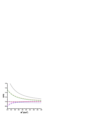
Figure 1: The OPE convergence for the $J^{PC}=0^{-+},~{}D_{s}D_{s0}$ molecule, in the region $2.2\leq M^{2}\leq 4.0~{}\nobreak\,\mbox{GeV}^{2}$ for $\sqrt{s_{0}}=5.2$ GeV. We plot the relative contributions starting with the perturbative contribution (solid line), and each other line represents the relative contribution after adding of one extra condensate in the expansion: + $D=3$ (dashed line), + $D=4$ (dotted line), + $D=5$ (solid line with circles), + $D=6$ (dashed line with squares), + $D=8$ (dotted line with triangles), + $D=10$ (solid line with triangles).

The continuum threshold is a physical parameter that should be determined from the spectrum of the mesons. The value of the continuum threshold in the QCDSR approach is, in general, given as the value of the mass of the first excitated state squared. In some known cases, like the $\rho$ and $J/\psi$, the first excitated state has a mass approximately $0.5~{}\nobreak\,\mbox{GeV}$ above the ground state mass. In the cases that one does not know the spectrum, one expects the continuum threshold to be approximately the square of the mass of the state plus $0.5~{}\nobreak\,\mbox{GeV}$: $s_{0}=(m_{0}+0.5~{}\nobreak\,\mbox{GeV})^{2}$. Therefore, to fix the continuum threshold range we extract the mass from the sum rule, for a given $s_{0}$, and accept such value of $s_{0}$ if the obtained mass is in the range 0.4 GeV to 0.6 GeV smaller than $\sqrt{s_{0}}$. Using this criterion, we obtain $s_{0}$ in the range $5.1\leq\sqrt{s_{0}}\leq 5.3~{}\nobreak\,\mbox{GeV}$.

The Borel window is determined by analysing the OPE convergence, the Borel stability and the pole contribution. To determine the minimum value of the Borel mass we impose that the contribution of the higher dimension condensate should be smaller than 10% of the total contribution: $M^{2}_{min}$ is such that

$$\left|{\mbox{OPE summed up dim n-1 }(M^{2}_{min})\over\mbox{total contribution }(M^{2}_{min})}\right|=0.9.$$ (11)

In Fig. 1 we show the relative contribution of all the terms in the OPE side of the sum rule, in the region $2.2\leq M^{2}\leq 4.0~{}\nobreak\,\mbox{GeV}^{2}$, for $\sqrt{s_{0}}=5.2~{}\nobreak\,\mbox{GeV}$. From this figure we see that the contribution of the dimension-10 condensate is smaller than 10% of the total contribution for values of $M^{2}\geq 2.4~{}\nobreak\,\mbox{GeV}^{2}$, and that we have an excellent OPE convergence for $M^{2}\geq 2.4~{}\nobreak\,\mbox{GeV}^{2}$. To have an idea of the importance of the different terms in the OPE, we show, in Fig. 2, the contribution of each condensate. As we can see, the condensates of dimension higher than six are, at least, one order of magnetude smaller than the perturbative contribution, in all considered Borel region.

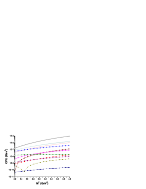
Figure 2: The OPE convergence for the $J^{PC}=0^{-+},~{}D_{s}D_{s0}$ molecule, in the region $2.2\leq M^{2}\leq 4.0~{}\nobreak\,\mbox{GeV}^{2}$ for $\sqrt{s_{0}}=5.2$ GeV. We plot the contributions of all individual condensates in the OPE: the perturbative contribution (solid line), $\langle\bar{s}s\rangle$ contribution (dashed line), $\langle g^{2}G^{2}\rangle$ contribution (dotted line), $m_{0}^{2}\langle\bar{s}s\rangle$ (solid line with cicles), $\langle\bar{s}s\rangle^{2}$ (dashed line with circles), $\langle g^{3}G^{3}\rangle$ (dotted line with circles), $m_{0}^{2}\langle\bar{s}s\rangle^{2}$ (solid line with squares), $\langle g^{2}G^{2}\rangle^{2}$ (dashed line with squares), $(m_{0}^{2}\langle\bar{s}s\rangle)^{2}$ (dotted line with squares), $\langle\bar{s}s\rangle^{2}\langle g^{2}G^{2}\rangle$ (dashed line with triangles), $\langle g^{2}G^{2}\rangle\langle g^{3}G^{3}\rangle$ (solid line with triangles).

Figure 3: The pseudoscalar meson mass, described with a $D_{s}D_{s0}$ molecular current, as a function of the sum rule parameter ($M^{2}$) for $\sqrt{s_{0}}=5.2$ GeV. The solid line shows the result obtained considering all contributions up to dimension-10. The dashed and dotted lines show, respectively, the results obtained neglecting the contributions of the dimension-8 ($\langle g^{2}G^{2}\rangle^{2}$) and dimension-10 ($\langle g^{2}G^{2}\rangle\langle g^{3}G^{3}\rangle,~{}\langle g^{2}G^{2}\rangle\langle\bar{s}s\rangle^{2}$) gluon condensates.

As commented above, the OPE convergence is very good in the Borel range $2.4\leq M^{2}\leq 4.0~{}\nobreak\,\mbox{GeV}^{2}$. However, the Borel stability for the mass of the state is only good for $M^{2}\geq 2.8~{}\nobreak\,\mbox{GeV}^{2}$, as can be seen through the solid line in Fig. 3. Therefore, we fix the lower value of $M^{2}$ in the sum rule window as $M^{2}_{min}=2.8$ GeV².

In Fig. 3 we also show, through the dashed and dotted lines, the result obtained if we neglect the contribution of dimension-8 and dimension-10 gluon condensates. We see that the contribution of the dimension-8 and -10 gluon condensates ($\langle g^{2}G^{2}\rangle^{2},~{}\langle g^{2}G^{2}\rangle\langle g^{3}G^{3}\rangle,~{}\langle g^{2}G^{2}\rangle\langle\bar{s}s\rangle^{2}$) are only important in the region $M^{2}\leq 2.8\nobreak\,\mbox{GeV}^{2}$, which is not in our Borel window, due to the mass stability. Therefore, at least in this case, the contribution of higher dimension gluon condensates could be safely neglected. Besides, as can be seen in Fig. 4, where we show the results for the mass for different values of $\sqrt{s_{0}}$ considering all condensate contributions up to dimension-10, the dependence of the mass on the OPE convergence is smaller than the its dependence on the continuum threshold parameter.

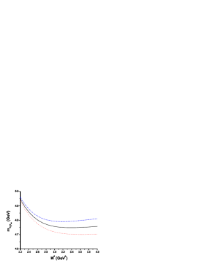
Figure 4: The pseudoscalar meson mass, described with a $D_{s}D_{s0}$ molecular current, as a function of the sum rule parameter ($M^{2}$) for $\sqrt{s_{0}}=5.1$ GeV (dotted line), $\sqrt{s_{0}}=5.2$ GeV (solid line) and $\sqrt{s_{0}}=5.3$ GeV (dot-dashed line).

To be able to extract, from the sum rule, information about the low-lying resonance, the pole contribution to the sum rule should be bigger than, or at least equal to, the continuum contribution. Since the continuum contribution increases with $M^{2}$, due to the dominance of the perturbative contribution, we fix the maximum value of the Borel mass to be the one for which the pole contribution is equal to the continuum contribution.

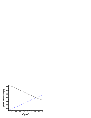
Figure 5: The solid line shows the relative pole contribution (the pole contribution divided by the total, pole plus continuum, contribution) and the dashed line shows the relative continuum contribution for $\sqrt{s_{0}}=5.2~{}\nobreak\,\mbox{GeV}$.

From Fig. 5 we see that for $\sqrt{s_{0}}=5.2~{}\nobreak\,\mbox{GeV}$, the pole contribution is bigger than the continuum contribution for $M^{2}\leq 3.66\nobreak\,\mbox{GeV}^{2}$. We show in Table I the values of $M_{max}$ for other values of $\sqrt{s_{0}}$. Although for $\sqrt{s_{0}}=5.0~{}\nobreak\,\mbox{GeV}$ there is still a small allowed Borel window, the difference between the obtained mass and the continuum threshold is very small (smaller than 0.2 GeV). Therefore, we do not consider values of $\sqrt{s_{0}}<5.1~{}\nobreak\,\mbox{GeV}$.

Table I: Upper limits in the Borel window for the $0^{-+},~{}D_{s}D_{s0}$ current obtained from the sum rule for different values of $\sqrt{s_{0}}$.
$\sqrt{s_{0}}~{}(\nobreak\,\mbox{GeV})$ $M^{2}_{max}(\nobreak\,\mbox{GeV}^{2})$ 5.1 3.43 5.2 3.66 5.3 3.90

To estimate the dependence of our results with the values of the quark masses and condensates, we fix $\sqrt{s_{0}}=5.2~{}\nobreak\,\mbox{GeV}$ and vary the other parameters in the ranges: $m_{c}=(1.23\pm 0.05)~{}\nobreak\,\mbox{GeV}$, $m_{s}=(0.13\pm 0.03)\,\nobreak\,\mbox{GeV}$, $\langle\bar{q}q\rangle=\,-(0.23\pm 0.03)^{3}\,\nobreak\,\mbox{GeV}^{3}$, $m_{0}^{2}=(0.8\pm 0.1)\nobreak\,\mbox{GeV}^{2}$. In our calculation we have assumed the factorization hypothesis. However, it is important to check how a violation of the factorization hypothesis would modify our results. To do that we multiply the contribution of the four-quark condensates of $D=6,8$ and $D=10$ in Eq. (QCD sum rule calculation for the charmonium-like structures in the $J/\psi\phi$ and $J/\psi\omega$ invariant mass spectra) by a factor $K$, and we vary $K$ in the range $0.5\leq K\leq 2$. The dependence of our results with all the variations mentioned above is show in Table II.

Table II: Values obtained for $m_{D_{s}D_{s0}}$, in the Borel window $3.0\leq M^{2}\leq 3.65~{}\nobreak\,\mbox{GeV}^{2}$, when the parameters vary in the ranges showed.
parameter $m_{D_{s}D_{s0}}~{}(\nobreak\,\mbox{GeV})$ $m_{c}=(1.23\pm 0.05)~{}\nobreak\,\mbox{GeV}$ $4.76\pm 0.07$ $m_{s}=(0.13\pm 0.03)\,\nobreak\,\mbox{GeV}$ $4.76\pm 0.06$ $\langle\bar{q}q\rangle=\,-(0.23\pm 0.03)^{3}\,\nobreak\,\mbox{GeV}^{3}$ $4.89\pm 0.27$ $m_{0}^{2}=(0.8\pm 0.1)\nobreak\,\mbox{GeV}^{2}$ $4.753\pm 0.003$ $0.5\leq K\leq 2$ $4.80\pm 0.11$

Taking into account the uncertainties given above and the uncertainties due to the continuum threshold parameter and due to the OPE convergence, we finally arrive at

$$m_{D_{s}D_{s0}}=(4.78\pm 0.54)~{}\nobreak\,\mbox{GeV},$$ (12)

which, considering the error, is still in agreement with the mass of the newly observed structure $Y(4274)$.

One can also deduce, from Eq. (7), the parameter $\lambda$ defined in Eq. (3). We get:

$$\lambda=\left(6.0\pm 3.9\right)\times 10^{-2}~{}\nobreak\,\mbox{GeV}^{5}.$$ (13)

This number is of the same order as the current-state coupling obtained in ref. Albuquerque:2009ak , where the $J^{PC}=0^{++}$ $D_{s}^{*}D_{s}^{*}$ molecular current was considered to describe the $Y(4140)$:

$$\lambda_{D_{s}^{*}D_{s}^{*}}=\left(4.22\pm 0.83\right)\times 10^{-2}~{}\nobreak\,\mbox{GeV}^{5}.$$ (14)

Therefore, we can conclude that the state can be well represented by the $J^{PC}=0^{-+}$ $D_{s}\bar{D}_{s0}$ molecular current

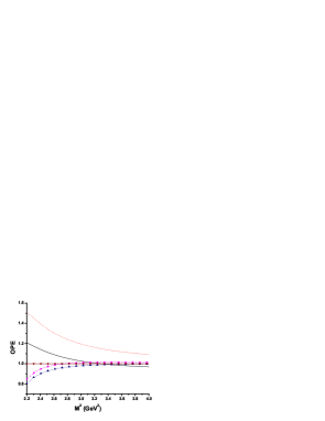
Figure 6: Same as Fig. 1 for the $DD_{0}$ current for $\sqrt{s_{0}}=5.0~{}\nobreak\,\mbox{GeV}$: perturbative contribution (long-dashed line), relative contribution after adding of one extra condensate in the expansion: + $D=4$ (dotted line), + $D=6$ (dashed line with squares), + $D=8$ (dotted line with triangles), + $D=10$ (solid line with triangles).

To obtain results for the $D\bar{D}_{0}$ molecular current with $J^{PC}=0^{-+}$, we only have to take $m_{s}=0$ and $\langle\bar{s}s\rangle=\langle\bar{q}q\rangle$ in Eq. (QCD sum rule calculation for the charmonium-like structures in the $J/\psi\phi$ and $J/\psi\omega$ invariant mass spectra). As can be seen by Fig. 6, the OPE convergence in this case is also very good for $M^{2}\geq 2.4~{}\nobreak\,\mbox{GeV}^{2}$. Therefore to fix the minimum value of the Borel parameter, we will consider the Borel stability of the obtained mass. For this we show, in Fig. 7 the results for the mass of the state described by a $DD_{0}$ pseudoscalar molecular current, for different values of $\sqrt{s_{0}}$. We see that for $M^{2}\geq 2.7~{}\nobreak\,\mbox{GeV}^{2}$ we get a good Borel stability. Therefore we fix $M^{2}_{min}=2.7~{}\nobreak\,\mbox{GeV}^{2}$.

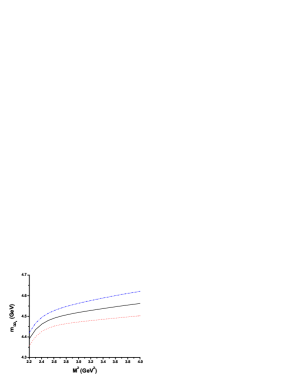
Figure 7: Same as Fig. 4 for the $DD_{0}$ molecular current, for $\sqrt{s_{0}}=4.9$ GeV (dotted line), $\sqrt{s_{0}}=5.0$ GeV (solid line) and $\sqrt{s_{0}}=5.1$ GeV (dot-dashed line).

In Table III we give the values of $M_{max}$ for the considered values of $\sqrt{s_{0}}$.

Table III: Upper limits in the Borel window for the $0^{-+},~{}DD_{0}$ current obtained from the sum rule for different values of $\sqrt{s_{0}}$.
$\sqrt{s_{0}}~{}(\nobreak\,\mbox{GeV})$ $M^{2}_{max}(\nobreak\,\mbox{GeV}^{2})$ 4.9 3.19 5.0 3.40 5.1 3.61

Taking into account the uncertainties due to the quark masses, condensates, continuum threshold parameter and OPE convergence, we finally arrive at

$$m_{DD_{0}}=(4.55\pm 0.49)~{}\nobreak\,\mbox{GeV},$$ (15)

which, although a little bigger than the prediction in ref. Liu:2010hf for a S-wave $D\bar{D}_{0}$ molecular state, is still in agreement with it, considering the error. It is interesting to notive that the result in Eq. (15) is in a excellent agreement with the result obtained in ref. Chen:2010jd , where different tetraquark currents were used to study $J^{PC}=0^{--}$ and $0^{-+}$ charmonium-like states. For the parameter $\lambda$ we get:

$$\lambda_{DD_{0}}=\left(5.4\pm 3.9\right)\times 10^{-2}~{}\nobreak\,\mbox{GeV}^{5}.$$ (16)

The mass we have obtained for the $D\bar{D}_{0}$ molecular state is approximately two hundred MeV below than the value obtained for the similar strange state. This is very different from the results obtained in ref. Albuquerque:2009ak where the $J^{PC}=0^{++}$ $D_{s}^{*}D_{s}^{*}$ and $D^{*}D^{*}$ molecular currents were considered. In the case of the scalar molecular currents, the difference between the masses of the strange and non-strange states was consistent with zero.

In conclusion, the newly observed structure $Y(4274)$ in the $J/\psi\phi$ invariant mass spectrum can be, considering the errors, interpreted as the S-wave $D_{s}\bar{D}_{s0}+h.c.$ molecular charmonium, in agreement with the findings in ref.  Liu:2010hf , where a dynamical study of the system, composed of the pseudoscalar and scalar charmed mesons, was done. In the case of the S-wave $D\bar{D}_{0}+h.c.$ molecular current, which was called as the cousin of $Y(4274)$ in ref.  Liu:2010hf , the QCDSR results are consistent with the enhancement structure around 4.2 GeV in the $J/\psi\omega$ invariant mass spectrum from $B$ decay Abe:2004zs .

References

• (1) S.-K. Choi et al. [Belle Collaboration], Phys. Rev. Lett. 91, 262001 (2003).
• (2) K. Abe et al. [Belle Collaboration], Phys. Rev. Lett. 100, 142001 (2008) [arXiv:0708.1790].
• (3) T. Aaltonen et al. [CDF Collaboration], arXiv:1101.6058.
• (4) T. Aaltonen et al. [CDF Collaboration], Phys. Rev. Lett.  102, 242002 (2009) [arXiv:0903.2229].
• (5) X. Liu, Z.G. Luo and S.-L. Zhu, arXiv:1011.1045.
• (6) K. Abe et al. [Belle Collaboration], Phys. Rev. Lett.  94, 182002 (2005) [arXiv:hep-ex/0408126].
• (7) B. Aubert et al. [BaBar Collaboration], Phys. Rev. Lett.  101, 082001 (2008) [arXiv:0711.2047].
• (8) X. Liu and S. L. Zhu, Phys. Rev. D 79, 094026 (2009) [arXiv:0903.2529].
• (9) X. Liu, Z. G. Luo, Y. R. Liu and S. L. Zhu, Eur. Phys. J. C 61, 411-428 (2009) [arXiv:0808.0073].
• (10) N. Mahajan, Phys. Lett.  B 679, 228 (2009) [arXiv:0903.3107].
• (11) Z. G. Wang, Eur. Phys. J.  C 63, 115 (2009) [arXiv:0903.5200].
• (12) T. Branz, T. Gutsche and V. E. Lyubovitskij, Phys. Rev.  D 80, 054019 (2009) [arXiv:0903.5424].
• (13) R. M. Albuquerque, M. E. Bracco and M. Nielsen, Phys. Lett.  B 678, 186 (2009) [arXiv:0903.5540].
• (14) X. Liu, Phys. Lett.  B 680, 137 (2009) [arXiv:0904.0136].
• (15) G. J. Ding, Eur. Phys. J.  C 64, 297 (2009) [arXiv:0904.1782].
• (16) J. R. Zhang and M. Q. Huang, J. Phys. G 37, 025005 (2010) [arXiv:0905.4178].
• (17) E. van Beveren and G. Rupp, arXiv:0906.2278.
• (18) F. Stancu, arXiv:0906.2485.
• (19) X. Liu and H. W. Ke, Phys. Rev.  D 80, 034009 (2009) [arXiv:0907.1349 [hep-ph]].
• (20) Z. G. Wang, Z. C. Liu and X. H. Zhang, Eur. Phys. J.  C 64, 373 (2009) [arXiv:0907.1467].
• (21) N. V. Drenska, R. Faccini and A. D. Polosa, Phys. Rev.  D 79, 077502 (2009) [arXiv:0902.2803].
• (22) R. Molina and E. Oset, Phys. Rev.  D 80, 114013 (2009) [arXiv:0907.3043].
• (23) M.A. Shifman, A.I. and Vainshtein and V.I. Zakharov, Nucl. Phys. B 147, 385 (1979).
• (24) L.J. Reinders, H. Rubinstein and S. Yazaki, Phys. Rept. 127, 1 (1985).
• (25) For a review and references to original works, see e.g., S. Narison, QCD as a theory of hadrons, Cambridge Monogr. Part. Phys. Nucl. Phys. Cosmol. 17, 1 (2002) [hep-h/0205006]; QCD spectral sum rules , World Sci. Lect. Notes Phys. 26, 1 (1989); Acta Phys. Pol. B 26, 687 (1995); Riv. Nuov. Cim. 10N2, 1 (1987); Phys. Rept. 84, 263 (1982).
• (26) M. Nielsen, F.S. Navarra, S.H Lee, Phys. Rep. 497, 41 (2010) [arXiv:0911.1958].
• (27) R.D. Matheus et al., Phys. Rev. D 75, 014005 (2007) [hep-ph/0608297].
• (28) S.H. Lee, A. Mihara, F.S. Navarra and M. Nielsen, Phys. Lett. B 661, 28 (2008) [arXiv:0710.1029].
• (29) S.H. Lee, M. Nielsen, U. Wiedner, Jour. Korean Phys. Soc. 55 (2009) 424 [arXiv:0803.1168].
• (30) M.E. Bracco, S.H. Lee, M. Nielsen, R. Rodrigues da Silva, Phys. Lett. B 671, 240 (2009) [arXiv:0807.3275].
• (31) R.M. Albuquerque and M. Nielsen, Nucl. Phys. A815, 53 (2009) [arXiv:0804.4817].
• (32) S.H. Lee, K. Morita and M. Nielsen, Nucl. Phys. A815, 29 (2009) [arXiv:0808.0690].
• (33) S.H. Lee, K. Morita and M. Nielsen, Phys. Rev. D78, 076001 (2008) [arXiv:0808.3168].
• (34) R.D. Matheus et al., Phys. Rev. D 80, 056002 (2009) [arXiv:0907.2683].
• (35) R.M. Albuquerque, J.M. Dias, M. Nielsen, Phys. Lett. B 690,141 (2010) [arXiv:1001.3092].
• (36) S. Narison, F.S. Navarra, M. Nielsen, Phys. Rev. D 83, 016004 (2011) [arXiv:1006.4802].
• (37) B. L. Ioffe, Nucl. Phys. B 188, 317 (1981); B 191, 591(E) (1981).
• (38) S. Narison, Phys. Lett. B 466, 345 (1999); Phys. Lett. B 361, 121 (1995); Phys. Lett. B 387, 162 (1996); Phys. Lett. B 624, 223 (2005).
• (39) J.R. Zhang and M. Q. Huang, Phys. Rev. D 80, 056004 (2009) [arXiv:0906.0090].
• (40) W. Chen and S.-L. Zhu, Phys. Rev. D 81, 105018 (2010) [arXiv:1003.3721].