Symmetry group analysis of an ideal plastic flow

Abstract

In this paper, we study the Lie point symmetry group of a system describing an ideal plastic plane flow in two dimensions in order to find analytical solutions. The infinitesimal generators that span the Lie algebra for this system are obtained. We completely classify the subalgebras of up to codimension two in conjugacy classes under the action of the symmetry group. Based on invariant forms, we use Ansatzes to compute symmetry reductions in such a way that the obtained solutions cover simultaneously many invariant and partially invariant solutions. We calculate solutions of the algebraic, trigonometric, inverse trigonometric and elliptic type. Some solutions depending on one or two arbitrary functions of one variable have also been found. In some cases, the shape of a potentially feasible extrusion die corresponding to the solution is deduced. These tools could be used to thin, curve, undulate or shape a ring in an ideal plastic material.

Running Title: Symmetry group analysis of an ideal plastic flow
PACS numbers: Primary 62.20.fq; Secondary 02.30.Jr
Keywords: symmetry group of partial differential equations, symmetry reduction, invariant solutions, ideal plasticity, extrusion die

I Introduction

In this paper, we investigate the plane flow of ideal plastic materials [1, 2, 3] modelled by the hyperbolic system of four partial differential equations (PDE) in $q=4$ dependent variables $\sigma,\theta,u,v$ and $p=2$ independent variables $x$ and $y$,

$$(a)\qquad \sigma_{x}-2k\left(\theta_{x}\cos 2\theta+\theta_{y}\sin 2\theta\right)=0,$$ (1)

$$(b)\qquad \sigma_{y}-2k\left(\theta_{x}\sin 2\theta-\theta_{y}\cos 2\theta\right)=0,$$

$$(c)\qquad (u_{y}+v_{x})\sin 2\theta+(u_{x}-v_{y})\cos 2\theta=0,$$

$$(d)\qquad u_{x}+v_{y}=0,$$

where $\sigma_{x}=\partial\sigma/\partial x$, etc. The expressions (LABEL:eq:1.a), (LABEL:eq:1.b), are the equilibrium equations for the plane problem. In other words they are the Cauchy differential equations of motion in a continuous medium where we consider that the sought quantities do not depend on $z$. These two equations involve the dependent variables $\sigma$ and $\theta$ that define the stress tensor; $\sigma$ is the mean pressure and $\theta$ is the angle relative to the $x$ axis in the counterclockwise direction minus $\pi/4$. The equation (LABEL:eq:1.c) corresponds, in the plane case, to the Saint-Venant-Von Mises plasticity theory equations, where $u$ and $v$ are respectively the velocities in the $x$ axis and $y$ axis directions. Moreover, we assume incompressibility of the material and hence the velocity vector is divergenceless. This explains the presence of the equation (LABEL:eq:1.d) in the considered system. The positive-definite constant $k$ is named the volumetric compression coefficient and is related to the Poisson coefficient and the Young modulus $\nu$ by the formula $k=(1-2\nu)E^{-1}$.

In order to calculate new solutions of the system consisting of (LABEL:eq:1.a) and (LABEL:eq:1.b), S.I. Senashov et al.[4, 5] acted with transformations of the symmetry group of this system on known solutions of some boundary value problems, i.e. the Nada solution [6] for a circular cavity under normal stress and shear and the Prandtl solution [7] for a bloc compressed between two plates. In addition, Czyz [8] found simple and double wave solutions for the system (LABEL:eq:1) using the method of characteristics. However, as it is often the case with this method, his solutions rely on numerical integration for obtaining the velocities $u$ and $v$. To our knowledge, no systematic Lie group analysis based on a complete subalgebra classification in conjugacy classes under the action of the symmetry group $G$ of the system (LABEL:eq:1) has been done before.

The goal of this paper is to systematically investigate the system (LABEL:eq:1) from the perspective of the Lie group of point symmetries $G$ in order to obtain analytical solutions. That is, we obtain in a systematic way all invariant and partially invariant (of structure defect $\delta=1$ in the sense defined by Ovsiannikov [9]) solutions under the action of $G$ which are non-equivalent. Invariant solutions are said non-equivalent if they cannot be obtained one from another by a transformation of $G$ (the solutions are not in the same orbit). In practice, we apply a procedure developed by J. Patera et al. [10, 11, 12] that consists of classifying the subalgebras of $\mathcal{L}$ associated with $G$ into conjugacy classes under the action of $G$. Two subalgebras $\mathcal{L}_{i}\subset\mathcal{L}$ and $\mathcal{L}_{i}^{\prime}\subset\mathcal{L}$ are conjugate if $G\mathcal{L}_{i}G=\mathcal{L}_{i}^{\prime}$. For each conjugacy class, we choose a representative subalgebra, find its invariants and use them to reduce the initial system (LABEL:eq:1) to a system in terms of the invariants which involve fewer variables. According to the approach proposed by Kruskal and Clarkson [13], which is part of the more general framework of conditional symmetries, we propose in this paper some Ansatzes which allow us to cover simultaneously many invariant and partially invariant solutions (PIS). These more general solutions reduce to invariant and partially invariant ones for appropriate parameter values. We illustrate these theoretical considerations with many classes of solutions. A more exhaustive collection of such solutions is provided in [14]. Thereafter, we draw for some solutions the shape of the corresponding extrusion die. The applied method relies on the fact that the walls of the tools must coincide with the flow lines describe by the velocities $u$ and $v$ of the solutions of the problem. In application, it is convenient to feed in material the extrusion die rectilinearly at constant speed. So, the tools illustrated in this paper were drawn considering this kind of feeding. Based on mass conservation and on the incompressibility of the materials, we easily deduce that the curve defining the limit of the plasticity region for constant feeding speed must obey the ordinary differential equation (ODE)

$$\frac{dy}{dx}=\frac{V_{0}-v(x,y)}{U_{0}-u(x,y)},$$ (2)

where $U_{0}$, $V_{0}$ are components of the feeding velocity of the die (or extraction velocity at the output of the die) respectively along the $x$-axis and $y$-axis. One should note that the conditions (2) are reduced to those required on the limits of the plasticity region in the paper of Czyz [8] when $V_{0}=0$ and that the curves defining the limits coincide with slip lines (characteristics), that it when we require $dy/dx=\tan\theta(x,y)$ or $dy/dx=-\cot\theta(x,y)$. Thus the condition (2) can be viewed as a relaxation of the boundary conditions given in the work of Czyz [8]. The reason we can use these relaxed conditions is that we choose the walls of the tool to coincide with the flow lines for a given solution rather than require the flow of material to be parallel to the walls. Using these relaxed conditions, we can choose (in some limits) the feeding speed and direction for a tool and this determines the limits of the plasticity region.

The paper is organized as follows. In section II we give the infinitesimal generators spanning the Lie algebra of symmetries $\mathcal{L}$ for the system (LABEL:eq:1) and the discrete transformations leaving it invariant. A brief discussion on the classification of subalgebras of $\mathcal{L}$ in conjugacy classes follows. Section III is concerned with symmetry reduction. It describes how the symmetry reduction method (SRM) has been applied to the system (LABEL:eq:1) and the method for finding partially invariant solutions. More precisely, we give several results obtained from Ansatzes so that each presented solution includes many invariant and partially invariant solutions corresponding to appropriate choices of the parameters. We conclude this paper with a discussion on the obtained results and some incoming results.

II Symmetry algebra and classification of its subalgebras

In this section we study the symmetries of the system (LABEL:eq:1). Following the standard algorithm [15], the Lie symmetry algebra of the system has been determined. It is spanned by the eight infinitesimal generators

$$\begin{gathered}D_{1}=x\partial_{x}+y\partial_{y},\qquad D_{2}=u\partial_{u}+v\partial_{v},\qquad B=-y\partial_{u}+x\partial_{v},\\ P_{1}=\partial_{x},\qquad P_{2}=\partial_{y},\qquad P_{3}=\partial_{\sigma},\qquad P_{4}=\partial_{u},\qquad P_{5}=\partial_{v},\end{gathered}$$ (3)

where we use the notation $\partial_{x}=\partial/\partial_{x}$, etc. The generators $D_{1}$ and $D_{2}$ generate dilations respectively in the space of independent variables $\left\{x,y\right\}$ and the space of dependent variables $\left\{u,v\right\}$. Moreover, $B$ is associated with a kind of boost and the $P_{i}$, $i=1,\ldots,5$ generate translations. The commutation relations for the generators (3) are shown in table I.

Table I: Commutation relations for the algebra $\mathcal{L}$.

$\mathcal{L}$	$D_{1}$	$D_{2}$	$B$	$P_{1}$	$P_{2}$	$P_{3}$	$P_{4}$	$P_{5}$
$D_{1}$	0	0	$B$	$-P_{1}$	$-P_{2}$	0	0	0
$D_{2}$	0	0	$-B$	0	0	0	$-P_{4}$	$-P_{5}$
$B$	$-B$	$B$	0	$-P_{5}$	$P_{4}$	0	0	0
$P_{1}$	$P_{1}$	0	$P_{5}$	0	0	0	0	0
$P_{2}$	$P_{2}$	0	$-P_{4}$	0	0	0	0	0
$P_{3}$	0	0	0	0	0	0	0	0
$P_{4}$	0	$P_{4}$	0	0	0	0	0	0
$P_{5}$	0	$P_{5}$	0	0	0	0	0	0

One should note that the system (LABEL:eq:1) is invariant under the discrete transformations:

$$R_{1}:\ x\mapsto-x,\quad y\mapsto-y,\quad \sigma\mapsto\sigma,\quad \theta\mapsto\theta,\quad u\mapsto u,\quad v\mapsto v;$$ (4)

$$R_{2}:\ x\mapsto x,\quad y\mapsto y,\quad \sigma\mapsto\sigma,\quad \theta\mapsto\theta,\quad u\mapsto-u,\quad v\mapsto-v.$$

These reflections induce the automorphisms of the Lie algebra $\mathcal{L}$:

$$\mathcal{R}_{1}: D_{1}\mapsto D_{1},\quad D_{2}\mapsto D_{2},\quad B\mapsto-B,\quad P_{1}\mapsto-P_{1},$$ (5)

$$P_{2}\mapsto-P_{2},\quad P_{3}\mapsto P_{3},\quad P_{4}\mapsto P_{4},\quad P_{5}\mapsto P_{5};$$

$$\mathcal{R}_{2}: D_{1}\mapsto D_{1},\quad D_{2}\mapsto D_{2},\quad B\mapsto-B,\quad P_{1}\mapsto P_{1},$$

$$P_{2}\mapsto P_{2},\quad P_{3}\mapsto P_{3},\quad P_{4}\mapsto-P_{4},\quad P_{5}\mapsto-P_{5}.$$

Since we seek solutions that are invariant and partially invariant of structure defect $\delta=1$, we only have to classify the subalgebras of codimension 1 and 2. We have used the following factorization of the Lie algebra $\mathcal{L}$:

$$\mathcal{L}=\left\{\left\{\left\{D_{1},D_{2}\right\}\rhd\left\{B\right\}\right\}\rhd\left\{P_{1},P_{2},P_{4},P_{5}\right\}\right\}\oplus\left\{P_{3}\right\},$$ (6)

where $\rhd$ denotes the semi-direct sum and $\oplus$ the direct sum of Lie algebras. The Lie algebra $\mathcal{L}$ is the direct sum of the center $\left\{P_{3}\right\}$ with the subalgebra $\{\{\{D_{1},D_{2}\}\rhd\{B\}\}\rhd\left\{P_{1},P_{2},P_{4},P_{5}\right\}\}$ which contains an abelian ideal $\left\{P_{1},P_{2},P_{4},P_{5}\right\}$. Applying the method [10, 11, 12], we proceed to classify all subalgebras of $\mathcal{L}$ in conjugacy classes under the action of the automorphisms generated by $G$ and the discrete transformations (LABEL:eq:3). In practice, we can classify the subalgebras under the automorphisms generated by $G$ and decrease the range of the parameters that appear in the representative subalgebra of a class using the Lie algebra automorphisms (5). The classification results are shown in table II for subalgebras of codimension 1 and in tables III and IV for subalgebras of codimension 2. For each subalgebra in these tables, a complete set of invariants is given. Table III contains the codimension 2 subalgebras which admit a symmetry variable, while table IV lists the codimension 2 subalgebras that have no symmetry variable. Despite the absence of a symmetry variable, the subalgebras in table IV lead to PIS.

III Symmetry reductions and solutions of the reduced systems.

In this section we use the symmetry reduction method, as presented in [15], to compute invariant solutions under the action of subgroups of the symmetry group $G$ of the initial system (LABEL:eq:1). Following the usual reduction procedure [16], we consider a subgroup $G_{d,j}\subset G$ associated with a subalgebra $\mathcal{L}_{d,j}\subset\mathcal{L}$ of dimension $d$. Then the subgroup $G_{d,j}$ admits $k=p+q-d$ functionally independent invariants $I=(I_{1}(x,u),\ldots,I_{k}(x,u))$, where $x$ denotes the for independent variables and $u$ the dependent variables. We have to consider three different possibilities.

• We first make the following hypotheses:

  • $q<d<p+q$,

  • the rank of the Jacobian matrix $(\partial I/\partial u)$ is $q$, i.e. $\operatorname{rank}(\partial I/\partial u)=q$,

  • the complete set of invariants under the action of $G_{d,j}$ takes the form
    $\{\xi_{1}(x),\ldots,\xi_{k-q}(x),I_{1}(x,u),\ldots,I_{q}(x,u)\}$, where $\xi_{i}$ denotes the symmetry variables.

  With these conditions, the invariant solutions under $G_{d,j}$ are in the form

  $$u_{i}=U_{i}(x,F(\xi)),\qquad i=1,\ldots,q,\qquad F(\xi)=(F_{1}(\xi),\ldots,F_{q}(\xi)),$$ (7)

  where $U=(U_{1},\ldots,U_{q})$ is the solution $u=(u_{1},\ldots,u_{q})$ of the relations

  $$F_{i}(\xi)=I_{i}(x,u),\qquad\xi=(\xi_{1}(x),\ldots,\xi_{k-q}).$$ (8)

  The $F_{i}$ functions that depend on the $k-q$ variables $\xi_{i}$, satisfy the differential equation system that results from the introduction of (7) into the system (LABEL:eq:1). To calculate the invariant solutions of the system (LABEL:eq:1), we must consider subalgebras of codimension $d=1$. Indeed, the system (LABEL:eq:1) is expressed in term of $p=2$ independent variables, so we cannot reduce it by more than one variable. In other words, we must have $k=5$ to apply the SRM to the system (LABEL:eq:1). This is possible only if $d=1$.

• Consider now the situation where $\operatorname{rank}(\partial I/\partial u)=q^{\prime}<q$ and $\{\xi_{1}(x),\ldots$, $\xi_{k-q^{\prime}}(x)$, $I_{1}(x,u),\ldots,I_{q^{\prime}}(x,u)\}$ is a complete set of invariants of $G_{d,j}$. In this case, it is only possible to solve the relations

  $$F_{j}(\xi)=I_{j}(x,u),\quad j=1,\ldots,q^{\prime},\qquad\xi=(\xi_{1},\ldots,\xi_{k-q^{\prime}}).$$ (9)

  for $q^{\prime}$ of the dependent variables $u$. Without loss of generality, we suppose that we solve the relations (9) for the first $q^{\prime}$ dependent variables $(u_{1},\ldots,u_{q^{\prime}})$. Then, introducing

  $$u_{i}=U_{i}(x,F(\xi)),\qquad i=1,\ldots,q^{\prime},\qquad F(\xi)=(F_{1}(\xi),\ldots,F_{q^{\prime}}(\xi)),$$ (10)

  into the system (LABEL:eq:1), we find a system of differential equations for the functions $F_{i}(\xi)$ in which we have the remaining $u_{q^{\prime}+1}(x),\ldots,u_{q}(x)$, which depend on the original independent variables $x$. We must add the compatibility conditions on the mixed derivatives of $u_{q^{\prime}+1},\ldots,u_{q}$. The obtained solutions are partially invariant. In this paper, we are interested in PIS of structure defect $\delta=1$ which are obtained from codimension 2 subalgebras. Subalgebras which satisfy the condition $\operatorname{rank}(\partial I/\partial u)=3<q$ are listed in table III.

• In the case where the subgroup $G_{d,j}$, corresponding to a codimension 2 subalgebra $L_{d,j}$, has a complete set of invariants satisfying the condition $\operatorname{rank}\left(\partial I/\partial u\right)=4$, there always exists, for the considered system (LABEL:eq:1), an invariant in terms of $x,y$ and $\sigma$ only. We denote this invariant $\tau$. Consequently, the set of invariants takes the form $\left\{\tau(x,y,\sigma),I_{1}(\theta,u,v),I_{2}(\theta,u,v),I_{3}(\theta,u,v)\right\}$ and we can solve for $\theta,u,v$ the relations

  $$F_{j}(\tau)=I_{j}(x,u),\qquad i=1,\ldots,3,$$ (11)

  and introduce the result in the system (LABEL:eq:1). To justify this particular choice for the invariant $\tau$ associated to $\mathcal{L}_{d,j}$, one should note that the equations (LABEL:eq:1.a), (LABEL:eq:1.b), do not involve the quantities $u$,$v$ and that the quantity $\theta$ is an invariant of the whole Lie algebra $\mathcal{L}$. This choice leaves the equations (LABEL:eq:1.a), (LABEL:eq:1.b), uncoupled to the equations (LABEL:eq:1.c), (LABEL:eq:1.d).

In the case of (i) and (ii), we can always choose the invariant $I_{1}=\theta$. Therefore, from the relations (9) we have

$$\theta(x,y)=J(\xi(x,y)),$$ (12)

where we write $F_{1}$ as $J$ for simplification. We will keep this notation for the subsequent sections of the paper. Introducing $\theta$ given by (12) in the equations (LABEL:eq:1.a), (LABEL:eq:1.b), and using the compatibility conditions on the mixed derivatives of $\sigma$ relative to $x$, $y$, we obtain an ODE for the function $J$. If we find the solution for $J$, the compatibility condition is satisfied and then we can integrate by quadrature to find the solution for $\sigma$. This solution is not necessarily an invariant one, but it includes invariant solutions for appropriate choices of parameters that appear in $\sigma$.

Concerning the case (iii), since there is no symmetry variable, we propose the solution for $\theta$ in the form

$$\theta(x,y)=J(\tau(x,y,\sigma(x,y))).$$ (13)

This allows one to solve the equations (LABEL:eq:1.a), (LABEL:eq:1.b), for $\theta$, $\sigma$, without considering the equations (LABEL:eq:1.c) and (LABEL:eq:1.d), because this leaves the equations uncoupled. None of the codimension 2 subalgebras of table IV admit a symmetry variable, but they possess an invariant in the form $\tau=h_{1}(x,y)\sigma+h_{2}(x,y)$. Thus, we can express $\sigma$ as

$$\sigma=\frac{\tau-h_{2}(x,y)}{h_{1}(x,y)}$$ (14)

and eliminate the quantities $\sigma$ from the equations (LABEL:eq:1.a), (LABEL:eq:1.b), and then use the compatibility condition on mixed derivatives relative to $x$ and $y$ of the function $\tau$ to obtain an ODE that must be verified by $J$. If we find the solution for $J$, we can find $\tau$ by quadrature and consequently we find $\sigma$ through the relation (14).

Below we present, for each distinct form of the symmetry variable $\xi$ or of the invariant $\tau$, the most general solution for $\theta$ and $\sigma$ of the equations (LABEL:eq:1.a), (LABEL:eq:1.b), where we suppose a solution for $\theta$ given by (12) or (13) depending on the considered case. Then for each of these solutions, we consider Ansatzes on the form of the velocities $u$ and $v$ to compute solutions that cover all invariants solutions corresponding to a given form of the symmetry variable $\xi$ or of the invariant $\tau$. In the table V, the subalgebras $\mathcal{L}_{i,j}$ are classified by symmetry variable and according to the form of the suggested Ansatz on the form of the solutions for $u$ and $v$. In general, the solutions are not necessarily invariant under the action of the symmetry group $G$ but they are so for an appropriate choice of integration constants. We illustrate with some examples the suggested method.

A Solution for $\theta$ in the form of a propagation wave.

The goal of this section is to construct a solution for the angle $\theta$ in the form of a propagation wave and to get the corresponding solution for the pressure $\sigma$ and then, in the subsections 1, 2, we get the velocities $u$ and $v$ from different assumptions made on the form of their solutions, i.e. we make additive separation and a multiplicative separation.

We look for a solution of the system (LABEL:eq:1.a), (LABEL:eq:1.b), such that $\theta(x,y)$ has the form

$$\theta(x,y)=J(\xi(x,y)),$$ (15)

with the function $J$ to determine and where

$$\xi(x,y)=a_{1}x+a_{2}y,\qquad a_{1},a_{2}\in\mathds{R}.$$ (16)

This type of solution includes, for appropriate values of the parameters $a_{1}$, $a_{2}$, all invariant and partially invariant solutions (for the quantities $\theta$, $\sigma$) corresponding to subalgebras $L_{1,j}$, $j=1,\ldots,4$ and $L_{2,k}$, $k=1,4,5,6,7,8,10,11$, (that is the subalgebras listed at line no. 1 in table V). Introducing (15), (16) in (LABEL:eq:1.a), (LABEL:eq:1.b), we get that the following system must be verified

$$(a)\qquad\sigma_{x}(x,y)=2k\left[a_{1}\cos(2J(\xi(x,y)))+a_{2}\sin(2J(\xi(x,y)))\right]J^{\prime}(\xi(x,y)),$$ (17)

$$(b)\qquad\sigma_{y}(x,y)=2k\left[a_{1}\sin(2J(\xi(x,y)))-a_{2}\cos(2J(\xi(x,y)))\right]J^{\prime}(\xi(x,y)).$$

The compatibility condition on the mixed derivatives for $\sigma$ relative to $x$ and $y$ provides the next ODE for $J$ in term of $\xi$

$$\left[-\lambda\sin(2J(\xi))+\mu\cos(2J(\xi))\right]J^{\prime\prime}(\xi)+\left[-2\mu\sin(2J(\xi))-2\lambda\cos(2J(\xi))\right]J^{\prime}(\xi)^{2}=0,$$ (18)

where $c_{1},c_{2}\in\mathds{R}$ are integration constants. The solution of (18) is

$$J(\xi)=\frac{1-s}{4}\pi+1/2\arctan\left(\frac{\mu(c_{1}\xi+c_{2})+\lambda\sqrt{\lambda^{2}+\mu^{2}-(c_{1}\xi+c_{2})^{2}}}{\lambda(c_{1}\xi+c_{2})-\mu\sqrt{\lambda^{2}+\mu^{2}-(c_{1}\xi+c_{2})^{2}}}\right),$$ (19)

where $s$ denote the sign of the expression $\lambda(c_{1}\xi+c_{2})-\mu\sqrt{\lambda^{2}+\mu^{2}-(c_{1}\xi+c_{2})^{2}}$ and $\lambda=a_{2}^{2}-a_{1}^{2}$, $\mu=-2a_{1}a_{2}$. The solution for $\theta(x,y)$ is provided by (15) with $J$ defined by (19) and $\xi(x,y)$ by (16). Thereafter, we substitute the solution (19) for $J$ in the system (LABEL:eq:9) and we solve for $\sigma$ by quadrature. We find the solution

$$\sigma(x,y)=-\frac{c_{1}k(a_{2}x-a_{1}y)}{a_{1}^{2}+a_{2}^{2}}-\frac{\sqrt{(a_{1}^{2}+a_{2}^{2})-\left(c_{1}(a_{1}x+a_{2}y)+c_{2}\right)^{2}}}{a_{1}^{2}+a_{2}^{2}}+c_{3},\quad c_{3}\in\mathds{R}.$$ (20)

We are interested in real solutions, so $\theta$ and $\sigma$ are defined over the domain

$$\Omega=\left\{(x,y):(a_{1}^{2}+a_{2}^{2})-\left(c_{1}(a_{1}x+a_{2}y)+c_{2}\right)^{2}>0\right\}.$$ (21)

Thus, we have that the quantities $\theta$ and $\sigma$ of all invariant solutions for the above subalgebras are covered by $\theta(x,y)=J(\xi(x,y))$ with $J$ defined by (19), $\xi(x,y)$ by (16) and $\sigma(x,y)$ by (20).

1 Additive separation for the velocities $u$ and $v$.

Corresponding to the solution for $\theta$ and $\sigma$ given respectively by (15), (16), (19) and by (20), we seek for a solution $u$ and $v$ of the additive separated form

$$u(x,y)=f(x,y)+F(\xi(x,y)),\qquad v(x,y)=g(x,y)+G(\xi(x,y)).$$ (22)

The first step is to classify the admissible forms for the functions $f$ and $g$. To do this, we substitute (22) in the system (LABEL:eq:1.c), (LABEL:eq:1.d), and we obtain the new system

$$(a)\qquad\left[f_{y}+a_{2}F^{\prime}(\xi(x,y))+g_{x}+a_{1}G^{\prime}(\xi(x,y))\right]\sin(2J(\xi(x,y)))$$ (23)

$$\qquad\qquad\quad+\left[f_{x}+a_{1}F^{\prime}(\xi(x,y))-g_{y}-a_{2}G^{\prime}(\xi(x,y))\right]\cos(2J(\xi(x,y)))=0,$$

$$(b)\qquad f_{x}+a_{1}F^{\prime}(\xi(x,y))+g_{y}+a_{2}G^{\prime}(\xi(x,y))=0,$$

where $F^{\prime}$, $G^{\prime}$ represent the derivative of $F$, $G$ relative to $\xi$ respectively. We will keep this notation in all of the following sections. We next introduce the linear differential operator

$$L_{\xi}=-a_{2}P_{1}+a_{1}P_{2}=-a_{2}\partial_{x}+a_{1}\partial_{y},$$ (24)

which annihilates any function in term of the quantity $\xi(x,y)=a_{1}x+a_{2}y$. Now, applying it to the system (LABEL:eq:15) we find the following conditions that constrain $f$ and $g$:

$$(a)\qquad\left(L_{\xi}(f_{y}+g_{x})\right)\sin(2J(\xi(x,y)))+2(L_{\xi}f_{x})\cos(2J(\xi(x,y)))=0,$$ (25)

$$(b)\qquad L_{\xi}(f_{x}+g_{y})=0.$$

Then, taking into account that $L_{\xi}$, $\partial_{x}$ and $\partial_{y}$ commute with each other and using the notation

$$\mathfrak{f}=L_{\xi}f,\qquad\mathfrak{g}=L_{\xi}g,$$ (26)

we can rewrite the conditions (LABEL:eq:17) in the new form

$$(a)\qquad \left(\mathfrak{f}_{y}+\mathfrak{g}_{x}\right)\sin(2J)+2\mathfrak{f}_{x}\cos(2J)=0,$$ (27)

$$(b)\qquad \mathfrak{f}_{x}+\mathfrak{g}_{y}=0.$$

We have to consider two cases separately, that is when $\mathfrak{f}$ and $\mathfrak{g}$ verify the equation (LABEL:eq:18.a) by requiring that the coefficients of the trigonometric functions vanish

$$\qquad\mathfrak{f}_{x}=\mathfrak{f}_{y}+\mathfrak{g}_{x}=0,$$ (28)

or by imposing that $\mathfrak{f}$ and $\mathfrak{g}$ obey the relation

$$\qquad\mathfrak{f}_{y}+\mathfrak{g}_{x}=-2\cot(2J(\xi))\mathfrak{f}_{x}.$$ (29)

(i)

If we suppose that (LABEL:eq:18.a) is satisfied by the conditions (28), then we have the following relations

$$(a)\qquad L_{\xi}f_{x}=0,$$ (30)

$$(b)\qquad L_{\xi}(f_{y}+g_{x})=0.$$

If $a_{1}\neq 0$, $a_{2}\neq 0$, the solution for $f$ and $g$ of (LABEL:eq:23) takes the form

$$f(x,y)=\zeta_{1}(\xi)+\omega_{1}y,\qquad g(x,y)=\zeta_{2}(\xi)+\omega_{2}x,\qquad\omega_{i}\in\mathds{R},\ i=1,2,3.$$ (31)

where the functions $\zeta_{i}$ are arbitrary functions of $\xi$. If $a_{1}=0$, then we can set $a_{2}=1$ without loss of generality. In this case, the functions $f$ and $g$ take the form

$$f(x,y)=\omega_{1}x+\zeta_{1}(y),\qquad g(x,y)=\omega_{2}x+\zeta_{2}(y),\qquad\omega_{i}\in\mathds{R},\ i=1,2.$$ (32)

where the function $\zeta_{i}$ are arbitrary functions of $y$. Similarly, we can consider the case $a_{1}=1$, $a_{2}=0$, which leads to the solutions

$$f(x,y)=\zeta_{1}(x)+\omega_{1}y,\qquad g(x,y)=\zeta_{2}(x)+\omega_{2}y,\qquad\omega_{i}\in\mathds{R},\ i=1,2,$$ (33)

where the functions $\zeta_{i}$ are arbitrary functions of $x$. Under the hypothesis (28), and according to appropriate values of $a_{i}$, the form for the functions $f$ and $g$ given by (31), (32) or (33), are the most general such that the Ansatz (22) reduces the system (LABEL:eq:1.c), (LABEL:eq:1.d), for $u$, $v$ to a system of two ODE for $F$ and $G$ in term of $\xi$ given by

$$F^{\prime}(\xi)=\frac{{a_{1}(f_{x}-g_{y})+a_{2}(f_{y}+g_{x})}\sin(2J(\xi))+2a_{2}f_{x}\cos(2J(\xi))}{(a_{2}^{2}-a_{1}^{2})\sin(2J(\xi))+2a_{1}a_{2}\cos(2J(\xi))},$$ (34)

$$G^{\prime}(\xi)=-a_{2}^{-1}\left(a_{1}F^{\prime}(\xi)+f_{x}+g_{y}\right).$$

We distinguish two different cases for the solutions $F$ and $G$ of (LABEL:eq:27), that is when $a_{1}\neq 0$ and $a_{2}\neq 0$ or when $a_{2}=0$.

(a)

If $a_{1}\neq 0$ and $a_{2}\neq 0$, we obtain

$$F(\xi)=-\zeta_{1}(\xi)+\frac{a_{1}(\omega_{1}+\omega_{2})\cos(2J(\xi))}{2c_{1}}+\frac{a_{2}\omega_{1}\sin(2J(\xi))}{c_{1}}+c_{4},$$ (35)

and

$$G(\xi)=-\zeta_{2}(\xi)-\frac{a_{1}^{2}(\omega_{1}+\omega_{2})\cos(2J(\xi))}{c_{1}}-\frac{a_{1}\omega_{1}\sin(2J(\xi))}{c_{1}}-\frac{\omega_{1}+\omega_{2}}{a_{2}}\xi+c_{5}.$$ (36)

Redefining the parameters $\omega_{1}$, $\omega_{2}$, the solutions $u$ and $v$ of (LABEL:eq:1.c), (LABEL:eq:1.d), are then

$$(a)\qquad u(x,y)=c_{4}x+\frac{a_{1}(c_{4}+c_{5})\cos(2J(\xi(x,y)))}{2c_{1}}+\frac{a_{2}c_{4}\sin(2(J(\xi(x,y))))}{c_{1}}+c_{6},$$ (37)

$$(b)\qquad v(x,y)=-\frac{a_{1}^{2}(c_{4}+c_{5})\cos(2J(\xi))}{2a_{2}c_{1}}-\frac{a_{1}c_{4}\sin(2J(\xi))}{c_{1}}-\frac{a_{1}(c_{4}+c_{5})x}{a_{2}}-c_{4}y+c_{7},$$

where the $c_{i}$ are integration constants. So, we obtain a solution of the system (LABEL:eq:1) by defining the angle $\theta$ by (15), (19), the pressure $\sigma$ by (20) and the velocities $u$ and $v$ by (LABEL:eq:31), with $\xi(x,y)=a_{1}x+a_{2}y$. As can be seen in the illustration, we plotted in figure 1 the shape of an extrusion die corresponding to the solution (LABEL:eq:31) for the velocities $u$ and $v$. The vector field defined by these velocities is traced inside the tool. The mean pressure in the extrusion die, which is given by (20), is represented by shades of grey, from pale grey for lower pressure to dark grey for higher pressure. The parameters have been set to $k=0.0027$, $a_{1}=1$, $a_{2}=1$, $c_{1}=0,5$, $c_{2}=0$, $c_{3}=0$, $c_{4}=0$, $c_{5}=-1$, $c_{6}=0$, $c_{7}=0$ and the feeding velocities modulus $U_{0}$, $U_{1}$, are both equal to $\sqrt{2}$, while the extraction velocities modulus $V_{0}$, $V_{1}$ are both equal to $\sqrt{3}$. The curves $C_{1}$, $C_{2}$ determine the limit of the plasticity region at the mouth of the die while the curves $C_{3}$, $C_{4}$, have the same meaning at the end of the die. It’s a double feeding tool which has a symmetric configuration under the reflection $x\mapsto-x$ except near the plasticity limits defined by $C_{3}$ and $C_{4}$. Other feeding and extraction settings are possible, that is the angle and the velocities modulus, but no setting with completely vertical extraction speeds were found.

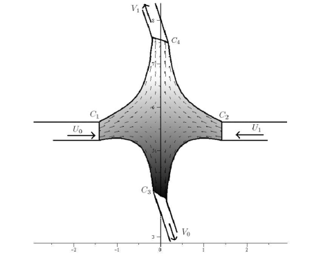
Figure 1: Extrusion die corresponding to the solution (20), (LABEL:eq:31).

(b)

Now, if $a_{1}=0$ and $a_{2}=1$, then $f$ and $g$ are given by (32). In this case, we find

$$F(y)=-\zeta_{1}(y)-\omega_{2}y-2\omega_{1}\int\cot 2J(y)dy+c_{4},$$ (38)

$$G(y)=-\omega_{1}y-\zeta_{2}(y)+c_{5}.$$

By redefining $\omega_{1}$, $\omega_{2}$, the solution may be written as

$$u(x,y)=c_{4}x-c_{5}y-2c_{4}\int\cot 2J(y)dy+c_{5},$$ (39)

$$v(x,y)=-c_{4}y+c_{7},$$

where the $c_{i}$ are real arbitrary constants. So, a solution of the system (LABEL:eq:1) consists of the angle $\theta$ by (15), (19), the pressure $\sigma$ by (20) and the velocities $u$ and $v$ by (LABEL:eq:33), with $\xi(x,y)=y$. For this solution, we did not trace an extrusion die because of the similarity with the next case where a tool will be plotted.

If $a_{1}=1$ and $a_{2}=0$, then the functions $f$ and $g$ are given by (33). We find in this case

$$F(x)=-\zeta_{1}(x)-\omega_{2}x+c_{4},$$ (40)

$$G(x)=-\omega_{1}x-\zeta_{2}(x)+2\omega_{2}\int\cot 2J(x)dx+c_{5}.$$

Redefining $\omega_{1}$, $\omega_{2}$, the solution for $u$ and $v$ of (LABEL:eq:1.c), (LABEL:eq:1.d) is

$$u(x,y)=-c_{5}x+c_{4}y+c_{6},$$ (41)

$$v(x,y)=-c_{4}x+c_{5}y+2c_{5}\int\cot 2J(x)dx+c_{7},$$

where the $c_{i}$ are real arbitrary constants. The system (LABEL:eq:1) is solved by the angle $\theta$ by (15), (19), the mean pressure $\sigma$ by (20) and the velocities $u$ and $v$ by (LABEL:eq:35), with $\xi(x,y)=x$.

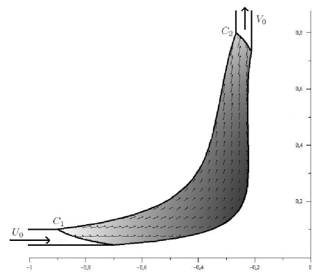
Figure 2: Extrusion die corresponding to the solution (20), (LABEL:eq:31).

An extrusion die corresponding to the solution (LABEL:eq:35), with the mean pressure provided by (20), is shown in figure 2 for parameter values set to $k=0.0027$, $a_{1}=1$, $a_{2}=0$, $c_{1}=0,5$, $c_{2}=0$, $c_{3}=0$, $c_{4}=-1$, $c_{5}=1$, $c_{6}=2$, $c_{7}=0$. The pressure is represented by the shades of grey ranging from pale to dark as the pressure increase. The curves $C_{1}$ and $C_{2}$ define the plasticity regions respectively at the mouth and at the end of the tool. The feeding velocity used is $U_{0}=1$ and the extraction velocity is $V_{0}=1$. For example, this die would be used to curve a plate or a rectangular rod.

(ii)

Now, we consider the case where $\mathfrak{f}$ and $\mathfrak{g}$ satisfy the condition (29). By the use of (LABEL:eq:18), the compatibility condition on $\mathfrak{g}$ leads to the hyperbolic equation

$$\mathfrak{f}_{xx}-\mathfrak{f}_{yy}-2\cot(2J(\xi))\mathfrak{f}_{xy}+4a_{2}\csc(2J(\xi))J^{\prime}(\xi)\mathfrak{f}_{x}=0,$$ (42)

over all the domain $\Omega$ defined by (21). So, we introduce the variables change $(x,y)$ to $(\varphi,\psi)$ defined by

$$\varphi=x+\frac{1}{c_{1}}\left(a_{1}\cos(2J)+a_{2}\sin(2J)-2J\right),$$ (43)

$$\psi=x+\frac{1}{c_{1}}\left(a_{1}\cos(2J)+a_{2}\sin(2J)+2J\right),$$

which enables us to rewrite (42) in the simplified form

$$\mathfrak{f}_{\varphi\psi}=\frac{c_{1}}{4a_{2}}(\mathfrak{f}_{\varphi}-\mathfrak{f}_{\psi})\cot(2J)+\frac{c_{1}}{4a_{2}}\frac{\mathfrak{f}_{\varphi}+\mathfrak{f}_{\psi}}{\sin(2J)}.$$ (44)

One should note that taking the difference of equations (LABEL:eq:37), we deduce

$$J=\frac{c_{1}(\psi-\varphi)}{4a_{2}}.$$ (45)

We can find a particular solution of (44) by assuming the solution in the separated form $\mathfrak{f}(\varphi,\psi)=P(K)+Q(J)$ where we use $K=\frac{c_{1}(\varphi+\psi)}{4a_{2}}$. Under such a hypothesis, the solution of the equation (LABEL:eq:37) is

$$\mathfrak{f}(\varphi,\psi)=\frac{\omega_{1}c_{1}}{4a_{2}}(\varphi+\psi)+\omega_{2}\cos\left(\frac{c_{1}(\psi-\varphi)}{2a_{2}}\right)+\frac{\omega_{1}}{2}\sin\left(\frac{c_{1}(\psi-\varphi)}{2a_{2}}\right)+\omega_{3},$$ (46)

where the $\omega_{i}\in\mathds{R},\ i=1,\ldots,3$, are integration constants. By considering the change of variable (LABEL:eq:37), the system (LABEL:eq:18) takes the form

$$\mathfrak{g}_{\varphi}=-\frac{\cos\left(\frac{c_{1}(\psi-\varphi)}{4a_{2}}\right)}{\sin\left(\frac{c_{1}(\psi-\varphi)}{4a_{2}}\right)}\mathfrak{f}_{\varphi},\qquad\mathfrak{g}_{\psi}=\frac{\sin\left(\frac{c_{1}(\psi-\varphi)}{4a_{2}}\right)}{\cos\left(\frac{c_{1}(\psi-\varphi)}{4a_{2}}\right)}\mathfrak{f}_{\psi},$$ (47)

from which we find the solution for $\mathfrak{g}$ defined by

$$\mathfrak{g}(\varphi,\psi)=-\frac{\omega_{1}}{2}\cos\left(\frac{c_{1}(\varphi-\psi)}{2a_{2}}\right)+\omega_{2}\sin\left(\frac{c_{1}(\varphi-\psi)}{2a_{2}}\right)-\frac{c_{1}\omega_{2}}{2a_{2}}(\varphi+\psi)+\omega_{4}.$$ (48)

where $\omega_{i}\in\mathds{R},\ i=1,\ldots,4$. Finally, returning to the initial variables and considering the relations (26), we obtain $f$ and $g$ defined by

$$f(x,y)= \frac{\omega_{1}c_{1}(2a_{1}\xi(x,y)-a_{2}\eta(x,y))\eta(x,y)}{4a_{2}(a_{1}^{2}+a_{2}^{2})}+\left(\left(\omega_{2}+\frac{\omega_{1}a_{1}}{2a_{2}}\right)\cos(2J(\xi(x,y)))\right.$$ (49)

$$\qquad\left.+\omega_{1}\sin(2J(\xi(x,y)))\right)\eta(x,y)+\omega_{3}\eta(x,y)+\zeta_{1}(\xi(x,y)),$$

$$g(x,y)= \frac{-\omega_{2}c_{1}(2a_{1}\xi(x,y)-a_{2}\eta(x,y))\eta(x,y)}{2a_{2}(a_{1}^{2}+a_{2}^{2})}-\left(\left(\frac{\omega_{1}}{2}+\frac{\omega_{2}a_{1}}{2}\right)\cos(2J(\xi(x,y)))\right)\eta(x,y)$$

$$\qquad+\omega_{4}\eta(x,y)+\zeta_{2}(\xi(x,y)),$$

where we introduced the notation

$$\xi(x,y)=a_{1}x+a_{2}y,\qquad\eta(x,y)=-a_{2}x+a_{1}y$$

and where $\zeta_{i}(\xi)$ are real arbitrary functions of one variable.

It remains for us to integrate the equations (LABEL:eq:15) with $f$ and $g$ given by (49), which form a system of two ODE for the unknown quantities $F$ and $G$ in term of $\xi$. The solution for $F$ is expressed by the quadrature

$$F(\xi)= \int\left[2a_{2}\kappa_{3}\left((a_{2}-1)\sin(2J)+2a_{1}\cos(2J)\right)\right]^{-1}$$ (50)

$$\times\Bigg{[}\omega_{1}\Big{(}-a_{1}c_{1}\left(\kappa_{1}\sin(2J(\xi))-2a_{2}\cos(2J(\xi))\right)\xi-\kappa_{3}\Big{(}2a_{2}\kappa_{1}\sin^{2}(2J(\xi))$$

$$+(a_{1}+3a_{2})\kappa_{2}\cos(2J(\xi))\sin(2J(\xi))-2a_{1}a_{2}\cos^{2}(2J(\xi))\Big{)}\Big{)}$$

$$+\omega_{2}\Big{(}-a_{1}c_{1}\kappa_{1}\xi\sin(2J(\xi))-2\kappa_{3}\cos(2J(\xi))\left(\kappa_{1}^{2}\sin(2J(\xi))-2a_{2}^{2}\cos(2J(\xi))\right)\Big{)}$$

$$\quad-2\omega_{3}a_{2}\kappa_{3}\left(\kappa_{1}\sin(2J(\xi))-2a_{2}\cos(2J(\xi))\right)+2\omega_{4}a_{2}\kappa_{1}\kappa_{3}\sin(2J(\xi))$$

$$+2\kappa_{3}a_{2}\Big{(}\left(\kappa_{2}\sin(2J(\xi))-2a_{1}\cos(2J(\xi))\right)\frac{d\zeta_{1}}{d\xi}-\kappa_{2}\sin(2J(\xi))\frac{d\zeta_{2}}{d\xi}\Big{)}\Bigg{]}d\xi+c_{4}.$$

It’s the same for the solution for $G$,

$$G(\xi)= \int\left[2a_{1}a_{2}\kappa_{3}\left((a_{2}-1)\sin(2J(\xi))+2a_{1}\cos(2J(\xi))\right)\right]^{-1}$$ (51)

$$\times\Bigg{[}\omega_{1}\Big{(}a_{1}c_{1}\xi\big{(}\left(a_{1}+a_{2}^{2}\right)\sin(2J(\xi))$$

$$+2a_{2}(a_{1}-1)\cos(2J(\xi))\big{)}+\kappa_{3}\big{(}2a_{2}(a_{1}+a_{2}^{3})\sin^{2}(2J(\xi))$$

$$+\left((6a_{1}-3)a_{2}^{2}+a_{1}^{2}\right)\big{)}\sin(2J(\xi))\cos(2J(\xi))+2a_{1}a_{2}(2a_{1}-1)\cos^{2}(2J(\xi))\Big{)}$$

$$+\omega_{2}\Big{(}2c_{1}a_{1}\left(a_{2}(a_{1}+1)\sin(2J(\xi))+2a_{1}^{2}\cos(2J(\xi))\right)\xi$$

$$+2\kappa_{3}\cos(2J(\xi))\big{(}a_{2}(a_{1}^{2}+2a_{1}+a_{2}^{2})\sin(2J(\xi))\left(2(a_{1}-1)a_{2}^{2}+2a_{1}^{3}\right)\cos(2J(\xi))\big{)}\Big{)}$$

$$+2\omega_{3}a_{2}\kappa_{3}\Big{(}(a_{1}+a_{2}^{2})\sin(2J(\xi))+2a_{2}(a_{1}-1)\cos(2J(\xi))\Big{)}$$

$$-2\omega_{4}a_{2}\kappa_{3}\Big{(}a_{2}(a_{1}+1)\sin(2J(\xi))+2a_{1}^{2}\cos(2J(\xi))\Big{)}$$

$$-2\kappa_{3}a_{2}(a_{1}-1)\Big{(}a_{2}\sin(2J(\xi))+2a_{1}\cos(2(2J(\xi)))\Big{)}\frac{d\zeta_{1}}{d\xi}$$

$$+\Big{(}(a_{2}^{2}-a_{1})\sin(2J(\xi))+2a_{1}a_{2}\cos(2J(\xi))\Big{)}\frac{d\zeta_{2}}{d\xi}\Bigg{]}d\xi+c_{5},$$

where we used $\kappa_{1}=a_{1}+a_{2}$, $\kappa_{2}=a_{1}-a_{2}$, $\kappa_{3}=a_{1}^{2}+a_{2}^{2}$. The functions $\zeta_{i}$ being arbitrary, they could be chosen in a way such that their derivatives $\partial\zeta_{i}/\partial\xi$ simplify the integration procedure for $F$ and $G$. Finally, the solutions for $u$ and $v$ are

$$u(x,y)=f(x,y)+F(a_{1}x+a_{2}y),\qquad v(x,y)=g(x,y)+G(a_{1}x+a_{2}y),$$ (52)

where the functions $f$ and $g$ are given by (49) while $F$ and $G$ are given respectively by the quadratures (50) and (51). So, we get a solution of the system (LABEL:eq:1) by defining the angle $\theta$ by (15), (19), the mean pressure $\sigma$ by (20) and the velocities $u$ and $v$ by (52), with $\xi(x,y)=a_{1}x+a_{2}y$.

2 Multiplicative separation for the velocities $u$ and $v$.

Considering the solution of (LABEL:eq:1.a), (LABEL:eq:1.b) for the angle $\theta$ provided by (15), (16), (19), and for the pressure $\sigma$ by (20), we now propose the solution for $u$ and $v$ to the equations (LABEL:eq:1.c), (LABEL:eq:1.d), in the multiplicative separated form

$$u(x,y)=f(x,y)F(\xi(x,y)),\qquad v(x,y)=g(x,y)G(\xi(x,y)),$$ (53)

where we suppose $f\neq 0$ and $g\neq 0$. For classifying the admissible $f$ and $g$, we substitute the velocities (53) into the system (LABEL:eq:1.c) and (LABEL:eq:1.d). This gives

$$(a)\qquad\left(f_{y}F(\xi(x,y))+a_{2}fF^{\prime}(\xi(x,y))+g_{x}G(\xi(x,y))+a_{1}gG^{\prime}(\xi(x,y))\right)\sin 2J(\xi(x,y))+$$ (54)

$$\qquad\qquad+\left(f_{x}F(\xi(x,y))+a_{1}fF^{\prime}(\xi(x,y))-g_{y}G(\xi)-a_{2}gG^{\prime}(\xi)\right)\cos 2J(\xi),$$

$$(b)\qquad f_{x}F(\xi(x,y))+a_{1}fF^{\prime}(\xi(x,y))+g_{y}G(\xi(x,y))+a_{2}gG^{\prime}(\xi(x,y))=0.$$

Applying to (LABEL:eq:45.b) the linear differential operator $L_{\xi}$ defined by (24), we have that the following equation must be satisfied

$$L_{\xi}\left(\frac{f_{x}}{g}\right)F+a_{1}L_{\xi}\left(\frac{f}{g}\right)F^{\prime}+L_{\xi}\left(\frac{g_{y}}{g}\right)G=0,$$ (55)

where we have $F=F(\xi(x,y))$, $G=G(\xi(x,y))$. In dealing with equation (55), there are three different cases to consider:

$$(i)\qquad L_{\xi}\left(\frac{f_{x}}{g}\right)=L_{\xi}\left(\frac{f}{g}\right)=L_{\xi}\left(\frac{g_{y}}{g}\right)=0,$$ (56)

$$(ii)\qquad L_{\xi}\left(\frac{g_{y}}{g}\right)=0,\qquad L_{\xi}\left(\frac{f}{g}\right)\neq 0,\qquad L_{\xi}\left(\frac{f_{x}}{g}\right)\neq 0$$

$$(iii) L_{\xi}\left(\frac{g_{y}}{g}\right)\neq 0.$$

(i)

In the first case, the functions $f$ and $g$ must take the form

$$f(x,y)=e^{\omega_{1}x}\zeta_{2}(\xi),\qquad g(x,y)=e^{\omega_{1}x}\zeta_{1}(\xi),\qquad\omega_{1}\in\mathds{R},$$ (57)

where $\omega_{1}$ corresponds to a damping factor when $\omega_{1}<0$. Introducing (57) in the system (LABEL:eq:45), we reduce this one to an ODE system for the functions $F$ and $G$ in term of $\xi$ from which we find

$$G(\xi)=A_{1}(\xi)F(\xi)+A_{2}(\xi)F^{\prime}(\xi),$$ (58)

where the coefficients $A_{i}(\xi)$, $i=1,2$, are given by

$$A_{1}(\xi)=\frac{1}{a_{2}\omega_{1}}\frac{\zeta_{2}(\xi)}{\zeta_{1}(\xi)}\left(\left(-2\omega_{1}a_{2}+\lambda\frac{\zeta_{2}^{\prime}}{\zeta_{2}}\right)\cot(2J(\xi))-\left(\mu\frac{\zeta_{2}^{\prime}}{\zeta_{2}}-a_{1}\omega_{1}\right)\right),$$ (59)

$$A_{2}(\xi)=\frac{1}{a_{2}\omega_{1}}\frac{\zeta_{2}(\xi)}{\zeta_{1}(\xi)}\left(\lambda\cot(2J(\xi))-\mu\right),$$

where $\zeta_{1}$, $\zeta_{2}$ are arbitrary functions of one variable, while the function $F$ must satisfy the ODE

$$F^{\prime\prime}(\xi)+\frac{\omega_{1}\zeta_{2}(\xi)+a_{1}\zeta_{2}^{\prime}(\xi)+a_{2}\zeta_{1}^{\prime}(\xi)A_{1}(\xi)+a_{2}\zeta_{1}(\xi)A_{1}^{\prime}(\xi)}{a_{2}\zeta_{1}(\xi)A_{2}(\xi)}F^{\prime}(\xi)$$ (60)

$$+\frac{a_{1}\zeta_{2}(\xi)+a_{2}\zeta_{1}^{\prime}(\xi)A_{2}(\xi)+a_{2}\zeta_{1}(\xi)(A_{1}(\xi)+A_{2}^{\prime}(\xi))}{a_{2}\zeta_{1}(\xi)A_{2}(\xi)}F(\xi)=0.$$

If we find the solution for $F$ of the equation (LABEL:eq:50) for a particular choice of the functions $\zeta_{1}$ and $\zeta_{2}$, then the solutions for the system (LABEL:eq:1.c), (LABEL:eq:1.d), for $u$ and $v$ will be given by (53) with $f$ and $g$ defined by (57) and $G$ by (58). However, by imposing $F(\xi)=\exp(K(\xi))$, the problem of solving (LABEL:eq:50) is reduced to the one of solving the Ricatti equation

$$K^{\prime\prime}(\xi)+K^{\prime}(\xi)^{2}+B_{1}(\xi)K^{\prime}(\xi)+B_{2}(\xi)=0,$$ (61)

where

$$B_{1}(\xi)= \frac{8a_{1}a_{2}J^{\prime}(\xi)^{2}}{c_{1}\sin(2J(\xi))}+\frac{2\zeta_{2}^{\prime}(\xi)}{\zeta_{2}(\xi)}+\frac{4\omega_{1}\left(a_{1}\sin(2J(\xi))-a_{2}\cos(2J(\xi))\right)J^{\prime}(\xi)}{c_{1}},$$

$$B_{2}(\xi)= \frac{\zeta^{\prime\prime}_{2}(\xi)}{\zeta_{2}(\xi)}+\frac{4J^{\prime}(\xi)\left(2a_{1}a_{2}J^{\prime}(\xi)+\omega_{1}a_{1}\sin(2J(\xi))^{2}-\omega_{1}a_{2}\sin(2J(\xi))\cos(2J(\xi))\right)\zeta_{2}^{\prime}(\xi)}{c_{1}\sin(2J(\xi))\zeta_{2}(\xi)}$$

$$+\frac{2\omega_{1}J^{\prime}(\xi)\left(4a_{2}J^{\prime}(\xi)+\omega_{1}\sin(2J(\xi))^{2}\right)}{c_{1}\sin(2J(\xi))}.$$

If we choose the function $\zeta_{2}$ to be a particular solution of the Ricatti equation obtained by imposing that the coefficient $B_{2}(\xi)\equiv 0$, then the ODE (61) becomes a nonlinear Bernoulli equation for $K^{\prime}(\xi)$ and the solution for $K(\xi)$ is obtained by quadrature. In this case, the solution for $F$ takes the form

$$F(\xi)=c_{4}\int\exp\left(-\int B_{1}(\xi)d\xi\right)d\xi+c_{5},\qquad c_{4},c_{5}\in\mathds{R}.$$ (62)

We substitute (62) in (58) and calculate the following solution for $G$:

$$G(\xi)=c_{4}\left[A_{1}(\xi)\int\exp\left(-\int B_{1}(\xi)d\xi\right)d\xi+A_{2}(\xi)\exp\left(-\int B_{1}(\xi)d\xi\right)\right]+c_{5}A_{2}(\xi).$$ (63)

Finally, the velocities $u$ and $v$ are

$$u(x,y)=e^{\omega_{1}x}\zeta_{2}(y/x)\left(c_{4}\int\exp\left(-\int^{\xi=y/x}B_{1}(\xi)d\xi\right)d\xi+c_{5}\right),$$ (64)

$$v(x,y)=e^{\omega_{1}x}\zeta_{1}(y/x)\left(c_{4}\left(A_{1}(y/x)\int^{\xi=y/x}e^{-\int B_{1}(\xi)d\xi}d\xi+A_{2}(\xi)e^{-\int B_{1}(\xi)d\xi}\right)+c_{5}A_{1}(\xi)\right),$$

where $A_{1}$, $A_{2}$ are defined by (LABEL:eq:49b), $\zeta_{1}(\xi)$ is an arbitrary function and $\zeta_{2}(\xi)$ is a solution of the Ricatti equation

$$\zeta^{\prime\prime}_{2}(\xi)+\frac{4J^{\prime}(\xi)\left(2a_{1}a_{2}J^{\prime}(\xi)+\omega_{1}a_{1}\sin(2J(\xi))^{2}-\omega_{1}a_{2}\sin(2J(\xi))\cos(2J(\xi))\right)\zeta_{2}^{\prime}(\xi)}{c_{1}\sin(2J(\xi))}$$

$$+\frac{2\omega_{1}J^{\prime}(\xi)\left(4a_{2}J^{\prime}(\xi)+\omega_{1}\sin(2J(\xi))^{2}\right)}{c_{1}\sin(2J(\xi))}\zeta_{2}(\xi)=0.$$

So, we have obtained a solution of the system (LABEL:eq:1) by redefining the angle $\theta$ by (15), (19), the pressure $\sigma$ by (20) and the velocities $u$ and $v$ by (LABEL:eq:50m4), with $\xi(x,y)=a_{1}x+a_{2}y$.

(ii)

In the second case, we have that

$$g(x,y)=\omega_{4}e^{\omega_{3}x}\zeta_{1}(\xi),\qquad\omega_{3},\omega_{4}\in\mathds{R},$$ (65)

and the function $f(x,y)$ must be a solution of the system of two PDE

$$f_{x}= -a_{1}\zeta_{2}^{\prime}(\xi)f+g\zeta_{3}(\xi)$$ (66)

$$f_{y}= -a_{2}\zeta_{2}^{\prime}(\xi)f-\omega_{3}\omega_{4}e^{\omega_{3}x}\left(\frac{\omega_{2}}{\omega_{1}}e^{-\zeta_{2}(\xi)}-\frac{\omega_{1}}{a_{2}}\int\zeta_{1}(\xi)\zeta_{3}(\xi)e^{\zeta_{2}(\xi)}d\xi\right)$$

$$+\omega_{4}e^{\omega_{3}x}\zeta_{1}(\xi)\zeta_{3}(\xi)\frac{-2a_{2}\cos(2J(\xi))+a_{1}\sin(2J(\xi))}{a_{2}\sin(2J(\xi))},$$

where the $\omega_{i}$, $i=1,2,3,4$, are real parameters and, in order that the system (66) be compatible, the functions $\zeta_{i}(\xi)$, $i=1,2,3$, must obey the condition

$$2\zeta_{1}(\xi)\zeta_{3}(\xi)\left(\frac{2a_{1}a_{2}J^{\prime}(\xi)}{\sin(2J(\xi))}-\omega_{3}\left(-a_{1}\sin(2J(\xi))+a_{2}\cos(2J(\xi))\right)\right)$$ (67)

$$+\left(\lambda\sin(2J(\xi))+\mu\cos(2J(\xi))\right)\left(\zeta_{1}(\xi)\zeta^{\prime}_{3}(\xi)+\zeta_{1}(\xi)\zeta_{3}(\xi)\zeta^{\prime}_{2}(\xi)+\zeta_{1}(\xi)\zeta^{\prime}_{1}(\xi)\right)$$

$$+\frac{a_{2}\omega_{3}^{2}}{\omega_{1}}e^{-\zeta_{2}(\xi)}\sin(2J(\xi))\left(-\omega_{2}+\frac{\omega_{1}}{a_{2}}\int\zeta_{1}(\xi)\zeta_{3}(\xi)e^{\zeta_{2}(\xi)}d\xi\right)=0.$$

The functions $F$ and $G$ are given by

$$F(\xi)=\omega_{1}e^{\zeta_{2}(\xi)},\qquad G(\xi)=\frac{1}{\zeta_{2}(\xi)}\left(\frac{-\omega_{1}}{a_{2}}\int\zeta_{1}(\xi)\zeta_{3}(\xi)e^{\zeta_{2}(\xi)}d\xi\right).$$ (68)

As an illustration, we compute an explicit solution of the system (LABEL:eq:1). To do this, we choose

$$\zeta_{2}(\xi)=-\ln(\zeta_{1}(\xi)),\qquad\zeta_{3}(\xi)=2\omega_{5}c_{1}^{-1}\sin(2J(\xi))J^{\prime}(\xi),\qquad\omega_{5}\in\mathds{R},$$ (69)

so that the equation (LABEL:eq:53) is verified and consequently the system (66) can be solved because it becomes compatible for $f$. The solution of the system (66) is then

$$f(x,y)=c_{1}^{-1}\left(2\omega_{4}\omega_{5}\int J^{\prime}(\xi)\sin(2J(\xi))dx+\frac{\omega_{4}\omega_{5}}{a_{1}a_{2}}y+\omega_{7}\right)\zeta_{1}(\xi),$$ (70)

where $\xi=a_{1}x+a_{2}y$ and the function $\zeta_{1}(\xi)$ has as its only restriction that its first derivative $d\zeta_{1}(\xi)/d\xi\neq 0$.

Finally, by introducing (65), (68) and (70) in the expression (53), with the function $\theta(x,y)$ defined by (15), (16) and (19), the solutions for $u$ and $v$ of the system (LABEL:eq:1.c), (LABEL:eq:1.d), are

$$u(x,y)=-c_{4}a_{2}\cos(2J(\xi))+c_{1}c_{4}y+c_{5},$$ (71)

$$v(x,y)=c_{4}a_{1}\cos(2J(\xi))+c_{6},\qquad c_{i}\in\mathds{R},\ i=1,2,3,4,$$

where the real parameters $\omega_{i}$ have been redefined to simplify the expression (LABEL:eq:57) in which the new parameters are $c_{i}$. So, we have a solution of the system (LABEL:eq:1) by defining the angle $\theta$ by (15), (19), the pressure $\sigma$ by (20) and the velocities $u$ and $v$ by (LABEL:eq:57), with $\xi(x,y)=a_{1}x+a_{2}y$.

(iii)

If the condition (LABEL:eq:47.iii) is satisfied, then we have

$$F(\xi)=\omega_{1}e^{-\zeta_{1}(\xi)/a_{1}},\qquad G(\xi)=-\omega_{1}\zeta_{2}(\xi)e^{-\zeta_{1}(\xi)/a_{1}},\quad\omega_{1}\in\mathds{R},$$ (72)

when the functions $f(x,y)$ and $g(x,y)$ are solutions of the system

$$f_{x}= \zeta^{\prime}_{1}(\xi)f+\zeta_{2}(\xi)g_{y}+f\zeta_{3}(\xi)g,$$ (73)

$$f_{y}= \frac{a_{2}}{a_{1}}\zeta^{\prime}_{1}(\xi)f+\zeta_{2}(\xi)g_{x}-2\cot(2J(\xi))\zeta_{2}(\xi)g_{y}$$

$$-\left(a_{1}a_{2}^{-1}-2\cot(2J(\xi))\right)\zeta_{3}(\xi)g,$$

where the functions $\zeta_{1}(\xi)$, $\zeta_{2}(\xi)$ are arbitrary and

$$\zeta_{3}(\xi)=a_{2}\left(-\frac{\zeta_{2}(\xi)\zeta^{\prime}_{1}(\xi)}{a_{1}}+\zeta^{\prime}_{2}(\xi)\right).$$ (74)

Using the compatibility condition on the mixed derivatives of the function $f(x,y)$ relative to $x$ and $y$, we obtain the second order ODE for $g(x,y)$

$$\zeta_{2}(\xi)\left(g_{xx}-g_{yy}-2\cot(2J(\xi))g_{xy}\right)-2\zeta_{3}(\xi)\left(a_{1}a_{2}^{-1}-\cot(2J(\xi))\right)g_{x}$$ (75)

$$+2\left(-\zeta_{3}(\xi)\left(1+a_{1}a_{2}^{-1}\cot(2J(\xi))\right)+\frac{2a_{1}\zeta_{2}(\xi)J^{\prime}(\xi)}{\sin^{2}(2J(\xi))}\right)g_{y}$$

$$+\left[\zeta_{3}(\xi)\left(\frac{4a_{1}J^{\prime}(\xi)}{\sin^{2}(2J(\xi))}+\zeta^{\prime}_{1}(\xi)\frac{\lambda-\mu\cot(2J(\xi))}{a_{1}a_{2}}\right)-\zeta^{\prime}_{3}(\xi)\left(\frac{\lambda-\mu\cot(2J(\xi))}{a_{2}}\right)\right]g=0.$$

It’s a hyperbolic equation on the domain $\Omega$ defined by (21). So the change of variable

$$(a)\qquad \phi(x,y)=x-\frac{2a_{2}J(\xi)}{c_{1}}+\frac{a_{1}(\cos(2J(\xi))+1)+a_{2}\sin(2J(\xi))}{c_{1}},$$ (76)

$$(b) \psi(x,y)=x+\frac{2a_{2}J(\xi)}{c_{1}}+\frac{a_{1}(\cos(2J(\xi))+1)+a_{2}\sin(2J(\xi))}{c_{1}},$$

transforms the equation (LABEL:eq:61) to the simplified form

$$0=g_{\phi\psi}(\phi,\psi)+\frac{c_{1}}{4a_{2}}\left(-\frac{\cos(2J(\xi))-1}{\sin(2J(\xi))}+\frac{\zeta_{3}(\xi)}{a_{2}\zeta_{2}(\xi)J^{\prime}(\xi)}\right)g_{\phi}(\phi,\psi)$$ (77)

$$+\frac{c_{1}}{4a_{2}}\left(\frac{\cos(2J(\xi))+1}{\sin(2J(\xi))}-\frac{\zeta_{3}(\xi)}{a_{2}\zeta_{2}(\xi)J^{\prime}(\xi)}\right)g_{\psi}(\phi,\psi)$$

$$-\frac{c_{1}}{2a_{2}^{2}}\left(\frac{a_{1}\zeta_{3}(\xi)}{\zeta_{2}(\xi)\sin(2J(\xi))}+\frac{\lambda\sin(2J(\xi))-\mu\cos(2J(\xi))}{4a_{2}a_{1}\zeta_{2}(\xi)J^{\prime}(\xi)}\left(\zeta_{3}(\xi)\zeta^{\prime}_{1}(\xi)-a_{1}\zeta^{\prime}_{3}(\xi)\right)\right)g(\phi,\psi)$$

Once again, if we take the difference of equations (LABEL:eq:62.a) and (LABEL:eq:62.b), we deduce the relation (45). In order to simplify the equation (LABEL:eq:63) and to solve it, we choose $\zeta_{3}(\xi)=0$. This is equivalent, considering (74), to requiring $-a_{1}^{-1}\zeta_{2}(\xi)\zeta^{\prime}_{1}(\xi)+\zeta^{\prime}_{2}(\xi)=0$, which is satisfied if we choose

$$\zeta_{2}(\xi)=\omega_{3}\exp(a_{1}^{-1}\zeta_{1}(\xi)).$$ (78)

So the equation (LABEL:eq:63) transforms to

$$g_{\phi\psi}+\frac{c_{1}\left(g_{\phi}+g_{\psi}\right)}{4a_{2}\sin(2J(\phi,\psi))}-\Bigg{(}a_{1}\sin(2J(\phi,\psi))+\frac{1}{2a_{2}}(a_{2}^{2}-a_{1}^{2})\cos(2J(\phi,\psi))$$ (79)

$$+\frac{c_{1}a_{1}}{\sin(2J)\left(-\lambda\sin(2J)+\mu\cos(2J(\phi,\psi))\right)}\Bigg{)}\left(g_{\phi}-g_{\psi}\right)=0.$$

We propose the solution of (LABEL:eq:66) in the form $g=g(J(\phi,\psi),K(\phi,\psi))$ with $J$ given by (45) and $K=(2a_{2})^{-1}c_{1}(\psi+\phi)$, which allows us to find the solution

$$g(\phi,\psi)=\omega_{3}\cos(2J(\phi,\psi))+\omega_{4}\sin(2J(\phi,\psi))-\frac{c_{1}\omega_{4}(\phi+\psi)}{2a_{2}}+\omega_{5}.$$ (80)

The solution expressed in term of $x$ and $y$ is

$$g(x,y)=\left(\omega_{3}-\frac{\omega_{4}a_{1}}{a_{2}}\right)\cos(2J(\xi))-\frac{\omega_{4}(xc_{1}+a_{1})}{a_{2}}+\omega_{5}.$$ (81)

Since the compatibility condition (LABEL:eq:66) is satisfied, the system (73) can be integrated after the substitution of $g(x,y)$ given by (81), $\zeta_{2}(\xi)$ by (78) and $\zeta_{3}(\xi)=0$. The solution for $f(x,y)$ is given by

$$f(x,y)=e^{\zeta_{1}(\xi)}\left(-\frac{\omega_{3}(-a_{2}\omega_{3}+\omega_{4}a_{1})\cos(2J(\xi))}{a_{1}}-\frac{c_{1}\omega_{3}^{2}y}{a_{1}}+\omega_{6}\right),$$ (82)

where $\zeta_{1}(\xi)$ is an arbitrary function of one variable and $\xi=a_{1}x+a_{2}y$. Finally, the solution for the system (LABEL:eq:1.c), (LABEL:eq:1.d), is obtained by introducing (72), (81) and (82) in (53). Redefining properly the parameters $\omega_{i}$, $i=3,4,5,6$, the solutions are

$$u(x,y)=c_{4}\left(-a_{2}\cos(2J(\xi))+c_{5}y\right)+c_{6},$$ (83)

$$v(x,y)=c_{4}\left(a_{1}\cos(2J(\xi))+(-c_{5}+c_{1})x\right)+c_{7},$$

where the $c_{i}$, $i=1,\ldots,7$ are integration constants. So, we have obtained a solution of the system (LABEL:eq:1) by defining the angle $\theta$ by (15), (19), the pressure $\sigma$ by (20) and the velocities $u$ and $v$ by (LABEL:eq:70), with $\xi(x,y)=a_{1}x+a_{2}y$. This solution includes the solution (LABEL:eq:57) to which it corresponds if we choose $c_{5}=c_{1}$ in (LABEL:eq:70). A extrusion die corresponding to the solution (LABEL:eq:70) is shown in figure 3. The parameter values that have been used are $k=0.8$, $c_{1}=2$, $c_{3}=1$, $a_{1}=-10$, $a_{2}=10$, $c_{4}=1$, $c_{5}=1$, $c_{6}=10$, $c_{7}=-10$. To demonstrate how the plasticity region changes when we vary the feeding velocities, we plotted two curves $C_{1}$ and $C_{2}$ to delimit the plasticity region at the mouth of the tool. The curve $C_{1}$ corresponds to a feeding velocity $U_{0}=3.54$ and the curve $C_{2}$ to a feeding velocity $U_{0}=3.84$, while the curve $C_{3}$ is the plasticity limit at the output and the extraction velocity is $U_{1}=16.12$. This kind of tool could be used to thin a plate for some ideal plastic material.

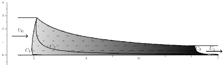
Figure 3: Extrusion die corresponding to the solution (20), (LABEL:eq:70).

B Similarity solution for the angle $\theta$ and corresponding pressure $\sigma$

In this section, we find solutions of the system (LABEL:eq:1) for which the angle $\theta$ is a similarity solution. We propose the solution for $\theta$ in the form provided by (15), but with the symmetry variable in the form

$$\xi(x,y)=y/x.$$ (84)

The solutions for $\theta$ and $\sigma$, which are obtained by this Ansatz, include for appropriate parameters choices the invariant solution corresponding to the subalgebras $\mathcal{L}_{1,j}$, $j$ ranging from 5 to 10 and $L_{2,k}$ for $k$ ranging from 13 to 27. The introduction of (15), with $\xi$ defined by (84), in the system (LABEL:eq:1.a), (LABEL:eq:1.b), leads to the system

$$\sigma_{x}(x,y)=2(k/x)\left(-\xi(x,y)\cos(J(\xi(x,y)))+\sin(\xi(x,y))\right)J^{\prime}(\xi(x,y)),$$ (85)

$$\sigma_{y}(x,y)=-2(k/x)\left(\xi(x,y)\sin(J(\xi(x,y)))+\cos(J(\xi(x,y)))\right)J^{\prime}(\xi(x,y)).$$

Considering the compatibility condition on mixed derivatives of $\sigma$ relative to $x$ and $y$, we deduce from (LABEL:eq:71) the following ODE for the function $J$:

$$\left((\xi^{2}-1)\sin(2J(\xi))+2\xi\cos(2J(\xi))\right)J^{\prime\prime}(\xi)+2\left(\xi\sin(2J(\xi))+\cos(J(\xi))\right)J^{\prime}(\xi)$$ (86)

$$+2\left(-2\sin(2J(\xi))+(\xi^{2}-1)\cos(2J(\xi))\right)(J^{\prime}(\xi))^{2}=0,$$

which has the first integral

$$\left((\xi^{2}-1)\sin(2J(\xi))+2\xi\cos(2J(\xi))\right)J^{\prime}(\xi)=c_{1},$$ (87)

where $c_{1}$ is an integration constant. There are two cases to consider to solve the equation (87).

i

If $c_{1}\neq 0$ the solution of (87) is given in implicit form by

$$\frac{\left(\tan(J(\xi))-\xi\right)\sqrt{c_{1}^{2}-1}}{\left(\tan(J(\xi))\xi+1\right)c_{1}-\xi+\tan(J(\xi))}-\tan\left(\frac{\sqrt{c_{1}^{2}-1}(c_{2}-J(\xi))}{c_{1}}\right)=0,$$ (88)

where $c_{2}$ is an integration constant. The solution for $\sigma$ is obtained by integrating the system (LABEL:eq:71) and taking into account the first integral (87). We find

$$\sigma(x,y)=k\left(\xi(x,y)\cos(2J(\xi(x,y)))-\sin(2J(\xi(x,y)))-2c_{1}\ln(x)\right)+c_{3},\quad c_{3}\in\mathds{R}$$ (89)

with $\xi(x,y)$ defined by (84) and $J(\xi)$ a solution of (88). So, $\theta(x,y)=J(y/x)$ and $\sigma(x,y)$ are given by (89) and are solutions of the system (LABEL:eq:1.a), (LABEL:eq:1.b), if the function $J(\xi)$ verify the algebraic equation (88).

ii

If the constant $c_{1}=0$ in the equation (88), then the solution of (LABEL:eq:72) for $J$ is

$$J(\xi)=-\frac{1}{2}\arctan\left(\frac{2\xi}{\xi^{2}-1}\right).$$ (90)

We subsequently solve (LABEL:eq:71) for $\sigma(x,y)$ considering (90), which leads to the solution of the system (LABEL:eq:1.a), (LABEL:eq:1.b), given by

$$\theta(x,y)=\frac{1}{2}\arctan\left(\frac{2xy}{x^{2}-y^{2}}\right),\qquad\sigma(x,y)=-2k\arctan\left(\frac{y}{x}\right)+c_{2}.$$ (91)

1 Additive separation for the velocities when $c_{1}\neq 0$.

Already knowing the solution $\theta(x,y)$, $\sigma(x,y)$, in the case of $c_{1}\neq 0$, we still have to compute the solution for $u$ and $v$. A way to proceed is to suppose that the solution is in the additive separated form

$$u(x,y)=f(x,y)+F(\xi(x,y)),\qquad v(x,y)=g(x,y)+G(\xi(x,y)),$$ (92)

where $\xi(x,y)=y/x$. We introduce (92) into the system (LABEL:eq:1.c), (LABEL:eq:1.d), which gives

$$\left(\sin(2J(\xi))-\cos(2J(\xi))\right)\xi F^{\prime}(\xi)-\left(\cos(2J(\xi))+\sin(2J(\xi))\right)\xi G^{\prime}(\xi)$$ (93)

$$+\left(\left(f_{y}+g_{x}\right)\sin(2J(\xi))+\left(f_{x}-g_{y}\right)\cos(2J(\xi))\right)x=0,$$

$$\left(f_{x}+g_{y}\right)x+G^{\prime}(\xi)-\xi F^{\prime}(\xi)=0,$$ (94)

We must determine which functions $f$ and $g$ will reduce the equations (LABEL:eq:79), (94), to a system of ODE for the one variable functions $F(\xi)$ and $G(\xi)$. To reach this goal, we first use as annihilator the infinitesimal generator $D_{1}$ defined by (3) that we apply to the equations (LABEL:eq:79), (94), to eliminate the presence of the functions $F$ and $G$. Indeed, $D_{1}$ annihilates any function of $\xi=y/x$. So, we obtain as differential consequences some conditions on the functions $f$ and $g$. We can assume $f_{x}(x,y)+g_{y}(x,y)\neq 0$, otherwise we can show that the only possible solution is the trivial constant solution for $u$ and $v$. Under this hypothesis, the previous conditions read

$$f_{x}=-g_{y}+\zeta_{1}(\xi)x^{-1},$$ (95)

$$f_{y}=-g_{x}+g_{y}\zeta_{2}(\xi)+\zeta_{3}(\xi)x^{-1},$$ (96)

$$\left(g_{y}+D_{1}\left(g_{y}\right)\right)\left(\zeta_{2}(\xi)\sin(2J(\xi))-2\cos(2J(\xi))\right)=0,$$ (97)

where the functions of one variable $\zeta_{i}$, $i=1,2,3$ are arbitrary. The left member of (97) being composed of two factors, we must consider two possibilities.

a.

We first suppose that

$$g_{y}+D_{1}\left(g_{y}\right)=0.$$ (98)

In this case, we find that the functions $f$ and $g$ take the form

$$f(x,y)= -\int^{\xi(x,y)}\frac{\zeta_{1}(\xi)-\zeta_{4}^{\prime}(\xi)}{\xi}d\xi+\omega_{4}\ln(y)-\omega_{1}y+\omega_{5},$$ (99)

$$g(x,y)= \zeta_{4}(\xi)+\omega_{2}\ln(x)+\omega_{1}x+\omega_{3},$$

where the functions $\zeta_{1}(\xi),\zeta_{4}(\xi)$ are arbitrary and the functions $\zeta_{2}(\xi)$, $\zeta_{3}(\xi)$, were chosen to solve the compatibility conditions on mixed derivatives of $f$ relative to $x$ and $y$. We now introduce the solution (99) in the system (95), (96), which leads to an ODE system for $F$ and $G$, that we omit due to its complexity, and for which the solutions take the form of quadratures

$$F(\xi)= \int\left(-\zeta^{\prime}_{4}(\xi)+\frac{\zeta_{1}(\xi)}{\xi}+\frac{(\omega_{4}+\omega_{2}\xi)\sin(2J(\xi))}{\xi\left((\xi^{2}-1)\sin(2J(\xi))+2\xi\cos(2J(\xi))\right)}\right)d\xi+c_{5},$$ (100)

$$G(\xi)= \int\left(-\zeta_{1}(\xi)+\xi F^{\prime}(\xi)\right)d\xi+c_{4},\qquad c_{4},c_{5}\in\mathds{R}.$$

The last step is to introduce (99) and (100) in the Ansatz (92). Then the velocities are

$$u(x,y)= -\frac{1}{2}\frac{c_{5}\cos(2J(y/x))}{c_{1}}+\int^{y/x}\frac{c_{6}\sin(2J(\xi))J^{\prime}(\xi)}{c_{1}\xi}d\xi+c_{6}\ln(y)-c_{4}y+c_{7},$$ (101)

$$v(x,y)= c_{5}\ln(x)+c_{4}x+\int^{y/x}c_{1}^{-1}c_{5}\xi\sin(2J(\xi))J^{\prime}(\xi)d\xi-\frac{1}{2}\frac{c_{6}\cos(2J(\xi))}{c_{1}}+c_{8}f,$$

where the $c_{i}$ are integration constants. So, we obtain a solution of the system (LABEL:eq:1) by defining the angle $\theta$ by (15), (88), the mean pressure $\sigma$ by (89) and the velocities $u$ and $v$ by (101), with $\xi(x,y)=y/x$.

b.

Suppose now that the condition (97) is satisfied by requiring

$$\zeta_{2}(\xi)=2\cot(2J(\xi)).$$ (102)

Then, applying the compatibility condition on mixed derivative of $f$ relative to $x$ and $y$ to the equations (95), (96), and considering $\zeta_{2}$ given by (102), we conclude that the function $g$ must solve the equation

$$g_{xx}(x,y)+2\cot(2J(\xi))g_{xy}(x,y)-g_{yy}(x,y)+4x^{-1}\xi\left(\xi+\cot^{2}(2J(\xi))\right)J^{\prime}(\xi)g_{y}(x,y)$$ (103)

$$+x^{-2}\left(\zeta^{\prime}_{3}(\xi)\xi+\zeta^{\prime}_{1}(\xi)+\zeta_{3}(\xi)\right)=0.$$

It’s a hyperbolic equation everywhere in the domain where $J$ is defined. So, we introduce the change of variable

$$\phi(x,y)= x\exp\left(\int^{\xi(x,y)}\frac{\sin(2J(\xi))}{1+\cos(2J(\xi))+\xi\sin(2J(\xi))}d\xi\right),$$ (104)

$$\psi(x,y)= x\exp\left(\int^{\xi(x,y)}\frac{\sin(2J(\xi))}{-1+\cos(2J(\xi))+\xi\sin(2J(\xi))}d\xi\right),$$

which brings the equation (LABEL:eq:90) to the simplified form

$$g_{\phi,\psi}+\frac{c_{1}}{2}\left(\frac{\sin(2J(\phi,\psi))g_{\phi}}{\psi(\cos(2J(\phi,\psi)))+1}-\frac{\sin(2J(\phi,\psi))g_{\psi}}{\phi(\cos(2J(\phi,\psi))-1)}\right)$$ (105)

$$-\frac{1}{4}\frac{\sin(2J(\phi,\psi))\xi^{2}-\sin(2J(\phi,\psi))+2\xi\cos(2J(\phi,\psi))\left(\zeta_{3}(\xi)+\zeta^{\prime}_{1}(\xi)+\xi\zeta^{\prime}_{3}(\xi)\right)}{\phi,\psi}=0,$$

where $J(\phi,\psi)$ is defined by (45). To solve the equation (LABEL:eq:92) more easily, we define the function $\zeta_{3}$ by

$$\zeta_{3}(\xi)=\frac{-\zeta_{1}(\xi)+J(\xi)+\omega_{1}}{\xi}.$$ (106)

So, the solution of (LABEL:eq:92) is

$$g(\phi,\psi)=-(1/2)\left(\omega_{1}-(1/2)\ln(\psi/\phi)\right)\cos\left(c_{1}\ln(\psi/\psi)\right)-(1/4)c_{1}^{-1}\sin\left(c_{1}\ln(\psi/\phi)\right),$$ (107)

which, returning to the initial variables, takes the form

$$g(x,y)=-(1/2)\left(\omega_{1}-(1/2)c_{1}^{-1}J(y/x)\right)\cos(2J(y/x))-(1/4)c_{1}^{-1}\sin(2J(y/x))+\omega_{2}.$$ (108)

After the introduction of the solution (108) for $g$, the function $f$ is given by quadrature from the equations (95), (96). The obtained solution for $f$ is

$$f(x,y)=\left(\int^{\xi(x,y)}\frac{\left(c_{1}\omega_{1}-J(\xi)\right)\sin(2J(\xi))J^{\prime}(\xi)}{c_{1}\xi}d\xi\right)-\int^{\xi(x,y)}\frac{\zeta_{1}(\xi)}{\xi}d\xi+(c_{1}+1)\omega_{1}\ln(y)+\omega_{3}.$$ (109)

We now introduce (108), (109), in (LABEL:eq:79), (94), and get $F$ and $G$ by quadrature in the form

$$F(\xi) =\int^{\xi(x,y)}\frac{\zeta_{1}(\xi)}{\xi}d\xi+\int^{\xi(x,y)}\frac{(\omega_{1}+J(\xi))\sin(2J(\xi))J^{\prime}(\xi)}{c_{1}\xi}d\xi,$$ (110)

$$G(\xi) =-(1/2)c_{1}^{-1}\left((\omega_{1}+J(\xi))\cos(2J(\xi))+2\sin(2J(\xi))\right).$$

Finally, the substitution of (108), (109) and (110) in (92) provides the solution to (LABEL:eq:1.c), (LABEL:eq:1.d):

$$u(x,y)= (c_{1}+1)c_{4}\ln(y)+\int^{y/x}\frac{c_{4}(c_{1}+1)\sin(2J(\xi))J^{\prime}(\xi)}{c_{1}\xi}d\xi+c_{5},$$ (111)

$$v(x,y)= -\frac{c_{4}(c_{1}+1)\cos(2J(y/x))}{c_{1}}+c_{6},$$

where the $c_{i}$ are integration constants. So, we have a solution of the system (LABEL:eq:1) by implicitly defining the angle $\theta$ by (15), (88), the mean pressure by $\sigma$ by (89) and the velocities $u$ and $v$ by (111), with $\xi(x,y)=y/x$.

2 Additive separation for the velocities $u$ and $v$ when $c_{1}=0$.

Now, we consider the case where $c_{1}=0$ in (87). Then the solutions for $\theta$ and $\sigma$ are given by (91). We still suppose the solution for $u$ and $v$ in the form (92). The procedure is the same as the previous case until we obtain the conditions (95), (96) and (97). We must again consider two distinct cases.

(a.)

We first suppose that the condition (98) is satisfied. Then, the functions $f$ and $g$ are defined by

$$f(x,y)= \int^{\xi(x,y)}(\zeta_{2}(\xi)+\xi)\zeta^{\prime}_{4}(\xi)-\zeta_{3}(\xi)d\xi-\omega_{1}y+\omega_{3},$$ (112)

$$g(x,y)= \zeta_{4}(\xi(x,y))+\omega_{1}x+\omega_{2},\qquad\omega_{i}\in\mathds{R},\ i=1,2,3,$$

where the $\zeta_{i}$, $=1,2,3$, are arbitrary functions of one variable and to simplify the expression for $f$ and $g$ we have chosen $\zeta_{1}(\xi)=\left(1-\zeta_{2}(\xi)\xi-\xi^{2}\right)\zeta_{4}(\xi)-\xi\zeta_{3}(\xi)$. We substitute (112) in the equations (LABEL:eq:79) and (94) to determine $F$ and $G$. We conclude that $F(\xi)$ is an arbitrary function, while $G(\xi)$ is expressed in term of a quadrature by

$$G(\xi)=\int\left(F^{\prime}(\xi)\xi+\left(\xi\zeta_{2}(\xi)-1+\xi^{2}\right)\zeta^{\prime}_{4}-\xi\zeta_{3}(\xi)\right)d\xi.$$ (113)

We finally obtain the solution $u$ and $v$ by introducing (112), (113) in (92) and, to simplify, by choosing

$$\zeta_{3}(\xi)=-\left(\zeta_{2}(\xi)+\xi\right)\zeta^{\prime}_{4}(\xi),$$

which gives

$$u(x,y)= -c_{2}y+F^{\prime}(y/x),$$ (114)

$$v(x,y)= c_{2}x+(y/x)F^{\prime}(y/x)-F(y/x),$$

where $F$ is a arbitrary function of one variable. A solution of the system (LABEL:eq:1) consists of the angle $\theta$ and the pressure $\sigma$ defined by (91) with the velocities defined by (114). For example, if we choose the arbitrary function to be an elliptic function, that is

$$F(\xi)=\operatorname{dn}\left(b_{1}\pi\left(1-e^{-b_{2}\xi^{2}}\right),\varrho\right),$$

and we set the parameters as $k=0.027$, $\epsilon=1$, $\omega_{1}=0$, $b_{1}=2$, $b_{2}=2$, $\varrho=1/2$, then we can trace (see figure 4) an extrusion die for a feeding speed of $U_{0}=0.75$ and an extraction speed $U_{1}=1$. The curve $C_{1}$ on the figure 4 delimits the plasticity region at the mouth of the tool, while the $x$-axis does the same for the output of the tool. This type of tool could be used to undulate a plate. We can shape the tool by varying the parameters. For example, we can vary the wave frequency setting the parameter $b_{1}$. Moreover, one should note that if the modulus $\varrho$ of the elliptic function is such that $0\leq\varrho^{2}\leq 1$, then the solution has one purely real and one purely imaginary period. For a real argument $\chi$, we have the relations

$$\sqrt{1-\varrho^{2}}\leq dn(\chi,\varrho)\leq 1.$$

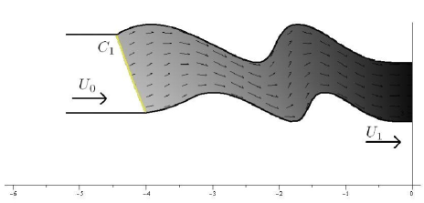
Figure 4: Extrusion die corresponding to the solution (20), (114).

b.

Suppose that $\zeta_{2}(\xi)$ is defined by (102) and for simplification we choose in particular

$$\zeta_{3}(\xi)=\frac{\zeta_{1}(\xi)}{\xi}.$$ (115)

Applying the mixed derivatives compatibility condition of $f$ to the equations (95), (96), we get the following ODE for the function $g$:

$$g_{xx}-g_{yy}-2\cot(2J(\xi))g_{xy}-\frac{4\xi J^{\prime}(\xi)g_{y}}{x\sin^{2}(2J(\xi))}=0.$$ (116)

By the change of variable

$$\xi(x,y)=y/x,\qquad\eta(x,y)=x^{2}+y^{2},$$ (117)

we reduce the PDE (116) in term of $x$ and $y$, to the much simpler PDE in term of $\xi$ and $\eta$,

$$g_{\xi\eta}+\frac{\xi g_{\eta}}{\xi^{2}+1}=0,$$ (118)

which has the solution

$$g(\xi,\eta)=\zeta_{4}(\xi)+\frac{\zeta_{5}(\eta)}{\sqrt{\xi^{2}+1}},$$ (119)

where $\zeta_{4}$ and $\zeta_{5}$ are arbitrary functions of one variable. Then, we find the solution for $f$ by integration of the PDE (95), (96), with $\zeta_{3}$ given by (115),

$$f(x,y)=-\int^{\xi(x,y)}\frac{\zeta_{1}(\xi)-\zeta^{\prime}_{4}(\xi)}{\xi}d\xi-\frac{y\zeta_{5}(\eta(x,y))}{\sqrt{\eta(x,y)}}+c_{2}.$$ (120)

By the substitution of (119) and (120) in the equations (LABEL:eq:79), (94), we find that $F$ is an arbitrary function of one variable and $G$ is defined by

$$G(\xi(x,y))=\int^{\xi(x,y)}\left(-\zeta_{1}(\xi)+F^{\prime}(\xi)\xi\right)d\xi+c_{3}.$$ (121)

So, we introduce (119), (120) and (121) in (92) and after an appropriate redefining of $\zeta_{1}$, $\zeta_{4}$ and $\zeta_{5}$, the solution to (LABEL:eq:1.c), (LABEL:eq:1.d) is provided by

$$u(x,y)=K^{\prime}(y/x)-yH(x^{2}+y^{2})+c_{2},\qquad v(x,y)=-K^{\prime}(y/x)+\xi K(\xi)+xH(x^{2}+y^{2})+c_{1},$$ (122)

where $H$, $K$ are arbitrary functions of one variable. The velocities (122) together with the angle and pressure defined by (91) solve the system (LABEL:eq:1). For example, a tool corresponding to the solution (122) with $H(\eta)=2\exp(-0.1\eta)$, $K(\xi)=\xi$ and for feeding and extraction speed given respectively by $U_{0}=1.05$ and $U_{1}=1.05$. It is shown in figure 5. The plasticity region limits correspond to the curves $C_{1}$ and $C_{2}$. This tool is symmetric under the reflection $x\mapsto-x$. Moreover, the top wall of the tool almost makes a complete loop, and this lets one suppose that we could make a ring in a material by extrusion.

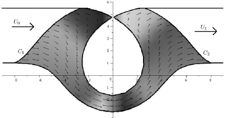
Figure 5: Extrusion die corresponding to the solution (20), (122).

3 Multiplicative separation for the velocities $u$ and $v$ when $c_{1}\neq 0$.

Consider the solutions of (LABEL:eq:1.a), (LABEL:eq:1.b), given by the angle $\theta(x,y)=J(y/x)$ with $J$ defined by (88) and the pressure $\sigma$ defined by (89). We require the solutions for $u$ and $v$ in the multiplicative separated form

$$u(x,y)=f(x,y)F(\xi(x,y)),\quad v(x,y)=g(x,y)G(\xi(x,y)),$$ (123)

where $\xi(x,y)=y/x$ and $f$, $g$, $F$, $G$ are to be determined. The Ansatz (123) on the velocities brings the system (LABEL:eq:1.c), (LABEL:eq:1.d) , to the form

$$\left[f_{y}F+x^{-1}fF^{\prime}(\xi)+g_{x}G(\xi)-x^{-1}\xi gG^{\prime}(\xi)\right]\sin(2J(\xi))$$ (124)

$$+\left[f_{x}F(\xi)-x^{-1}\xi fF^{\prime}-g_{y}G-x^{-1}gG^{\prime}\right]\cos(2J(\xi))=0,$$

$$\left[f_{x}F(\xi)+g_{y}G(\xi)\right]-\xi fF^{\prime}(\xi)+gG^{\prime}(\xi)=0.$$

To reduce the PDE system (LABEL:eq:ms:2) to an ODE system involving $F$ and $G$ in term of $\xi$, we act with the operator $D_{1}$, defined by (3), and annihilate the function of $\xi$ present in (LABEL:eq:ms:2). This leads to conditions on $f$ and $g$ that do not involve $F$, $G$ and their derivatives. There are three cases to consider, that is

$$(a)\quad D_{1}\left(g_{y}/g\right)\neq 0,\qquad D_{1}\left(\frac{D_{1}(f/g)}{D_{1}(xg_{y}/g)}\right)\neq 0,$$ (125)

$$(b)\quad D_{1}\left(xg_{y}/g\right)\neq 0,\qquad D_{1}\left(\frac{D_{1}(f/g)}{D_{1}(xg_{y}/g)}\right)=0,$$

$$(c)\quad D_{1}(xg_{y}/g)=0.$$

In this paper, we present the details for the cases (a) and (c).

(a)

We first suppose that the condition (LABEL:eq:ms:3.a) is satisfied. In this case, the function $f$ must be solution of the PDE system

$$f_{x}= -x^{-1}\xi\zeta_{1}(\xi)f+\zeta_{2}(\xi)g_{y}-x^{-1}\left(\zeta_{2}(\xi)\zeta_{1}^{\prime}(\xi)-\zeta_{2}^{\prime}(\xi)\right)g,$$ (126)

$$f_{y}= x^{-1}\zeta_{1}(\xi)f+\zeta_{2}(\xi)g_{x}-2\zeta_{2}(\xi)\cot(2J(\xi))g_{y}$$

$$+\left(\zeta_{2}(\xi)\zeta_{1}^{\prime}(\xi)-\zeta_{2}^{\prime}(\xi)\right)\frac{\xi\sin(2J(\xi))+2\cos(2J(\xi))}{x\sin(2J(\xi))}g,$$

where $\zeta_{1}$, $\zeta_{2}$ are two arbitrary functions of one variable. For the system (126) to be compatible, the function $g$ must satisfy the PDE

$$g_{xx}-2\cot(2J(\xi))g_{xy}-g_{yy}+2x^{-1}\zeta_{2}(\xi)^{-1}\left(\xi+\cot(2J(\xi))\right)\zeta_{3}(\xi)g_{x}$$ (127)

$$+2x^{-1}\left[\left(\xi-\cot(2J(\xi))\right)\zeta_{3}(\xi)-2\xi\sin^{-2}(J(\xi))J^{\prime}(\xi)\right]g_{y}$$

$$+x^{-2}\zeta_{2}(\xi)^{-1}\Big{(}[4\xi J^{\prime}(\xi)\sin^{-2}(2J(\xi))+\left(\xi^{2}-1+2\xi\cot(2J(\xi))\right)\zeta_{1}^{\prime}(\xi)$$

$$-2\xi-2\cot(2J(\xi))]\zeta_{3}(\xi)-\left(\xi^{2}-1+2\xi\cot(2J(\xi))\right)\zeta_{3}^{\prime}(\xi)\Big{)}g=0,$$

where we used the notation $\zeta_{3}(\xi)=\zeta_{2}(\xi)\zeta_{1}^{\prime}(\xi)-\zeta_{2}^{\prime}(\xi)$ to shorten the expression. The equation (LABEL:eq:ms:5) is difficult to solve for arbitrary $\zeta_{1}$, $\zeta_{2}$, but if we make the particular choice

$$\zeta_{2}(\xi)=\omega_{2}\exp(\zeta_{1}(\xi)),\qquad\omega_{2}\in\mathds{R},$$ (128)

then the PDE (LABEL:eq:ms:5) reduces to

$$g_{xx}-2\cot(2J(\xi))g_{xy}-g_{yy}-4x^{-1}\xi J^{\prime}(\xi)\sin^{-2}(J(\xi))g_{y}=0,$$ (129)

which is solved by the function

$$g(x,y)=\omega_{3}x+\omega_{4}\cos(2J(y/x))+\omega_{5},\quad\omega_{3},\omega_{4},\omega_{5}\in\mathds{R}.$$ (130)

With $g$ given by (130) and $\zeta_{2}(\xi)$ by (128), the system (126) is compatible. Consequently, $f$ is expressed in term of a quadrature. We find

$$f(x,y)= 2\exp(\zeta_{1}(y/x))\omega_{2}\omega_{4}\int^{y/x}\xi^{-1}\sin(2J(\xi))J^{\prime}(\xi)d\xi$$ (131)

$$+\exp(\zeta_{1}(y/x))\left(\omega_{2}\omega_{3}+2\omega_{2}\omega_{4}c_{1}\ln(y)+\omega_{6}\right)$$

With $f$ given by (131) and $g$ by (130), the solutions for $F$ and $G$ of the system (LABEL:eq:ms:2) are

$$F(\xi)=\omega_{1}\exp(-\zeta_{1}(\xi)),\qquad G(\xi)=\omega_{2}.$$ (132)

By introducing (130), (131), (132) in (123) and redefining the free parameters $\omega_{i}$, $i=1,2,3,4$, the solutions of (LABEL:eq:1.c), (LABEL:eq:1.d), for the velocities $u$ and $v$ is

$$u(x,y)=2c_{4}\int^{y/x}\xi^{-1}\sin(2J(\xi))J^{\prime}(\xi)d\xi+c_{5}y+2c_{1}c_{4}\ln(y)+c_{6},$$ (133)

$$v(x,y)=-c_{5}x-c_{4}\cos(2J(y/x))+c_{7},$$

where the $c_{i}$, $i=1,\ldots,7$, are integration constants and $J$ is defined by (88). So, we have a solution of the system (LABEL:eq:1) composed of the angle $\theta$ in the form (15) with $J$ given implicitly by (88) together with the pressure $\sigma$ (89) and the velocities (LABEL:eq:ms:11).

(c)

Suppose now that the condition(LABEL:eq:ms:3.c) is satisfied. In this case, the solution $g$ takes the form

$$g(x,y)=h_{1}(x)\zeta_{1}(\xi(x,y))$$ (134)

and the function $f$ must be solution of

$$f_{x}= x^{-1}\xi\zeta_{2}^{\prime}(\xi)f+x^{-1}\zeta_{3}(\xi)h_{1}(x),$$ (135)

$$f_{y}= -2x^{-1}h_{1}(x)\zeta_{3}(\xi)\cot(2J(\xi))+e^{-\zeta_{2}(\xi)}\left(\int^{y/x}e^{\zeta_{2}(\xi)}\zeta_{3}(\xi)d\xi-\omega_{2}\right)h_{1}^{\prime}(x)$$

$$-x^{-1}\left[\zeta_{2}^{\prime}(\xi)+\xi\zeta_{3}(\xi)\right].$$

We omit, due to its complexity, the expression of the compatibility condition on the mixed derivative of $f$ relative to $x$ and $y$. Nevertheless, making the specific choice

$$h_{1}(x)=1,\qquad\zeta_{2}(\xi)=\ln\left(\frac{\sin(2J(\xi))}{(\xi^{2}-1)\sin(2J(\xi))+2\xi\cos(2J(\xi))}\right)-\ln(\zeta_{3}(\xi)),$$ (136)

the system (135) turns out to be compatible and the solution to (135) is

$$f(x,y)= \zeta_{3}(y/x)\bigg{(}c_{1}^{-1}\left(1-(y/x)^{2}-2(y/x)\cot(2J(y/x))\right)\int^{y/x}\xi^{-1}\sin(2J(\xi))J^{\prime}(\xi)d\xi$$ (137)

$$+\left[1-(y/x)^{2}-2(y/x)\cot(2J(y/x))\right](\ln y-\omega_{4})\bigg{)}.$$

The substitution of (137), (134) and (136) in the system (LABEL:eq:ms:2) results in an ODE system for $F$ and $G$, omitted due to its complexity, which has the solution

$$F(\xi)=\frac{\omega_{1}\sin(2J(\xi))}{\zeta_{3}(\xi)\left((\xi^{2}-1)\sin(2J(\xi))+2\xi\cos(J(\xi))\right)},$$ (138)

$$G(\xi)=\zeta_{1}(\xi)^{-1}\left(\omega_{1}\cos(2J(\xi))-\omega_{2}\right).$$

We finally, obtain a solution for the system (LABEL:eq:1.c), (LABEL:eq:1.d), by the substitution of (137) and (LABEL:eq:ms:16), with $h_{1}(x)$, $\zeta_{2}(\xi)$, defined by (136), in (123). This leads to

$$u(x,y)=-c_{4}\ln(y)-c_{1}^{-1}c_{4}\int^{y/x}\xi^{-1}\sin(2J(\xi))J^{\prime}(\xi)d\xi+c_{5},$$ (139)

$$v(x,y)=(1/2)c_{1}^{-1}\omega_{1}\cos(2J(y/x))+c_{6},\qquad c_{1},c_{4},c_{5},c_{6}\in\mathds{R}.$$

So, the system (LABEL:eq:1) is solved by the angle $\theta$ in the form (15) with $J$ implicitly defined by (88), together with the pressure $\sigma$ (89) and the velocities (LABEL:eq:ms:17).

4 Multiplicative separation for the velocities $u$ and $v$ when $c_{1}=0$.

Consider now the case where $c_{1}=0$ in (87) so the solution of (LABEL:eq:1.a), (LABEL:eq:1.b), for $\theta$ and $\sigma$ is (91). We suppose that the velocities $u$ and $v$ are in the form (123). Introducing this form for the velocities and $\theta$ defined by (91) in the equations (LABEL:eq:1.c), (LABEL:eq:1.d), leads to the system (LABEL:eq:ms:2) which reduces to a ODE system for $F$ and $G$ if the functions $f$ and $g$ satisfy the condition (LABEL:eq:ms:3). The three different constraints (LABEL:eq:ms:3) must be considered separately.

(a)

In the first case, where we consider that the conditions (LABEL:eq:ms:3.a) are satisfied, the functions $f$ and $g$ must verify the system (126), (LABEL:eq:ms:5). Changing the variables $(x,y)$ to new variables $(\xi,\eta)$ defined by

$$\xi(x,y)=y/x,\qquad\eta(x,y)=x^{2}+y^{2},$$ (140)

and considering $\theta$ given by (91), the system (126),(LABEL:eq:ms:5), becomes

$$f_{\xi}=-\zeta_{1}(\xi)f-\xi^{-1}\zeta_{2}g_{\xi}-\xi^{-1}\left(\zeta_{2}^{\prime}(\xi)-\zeta_{1}(\xi)\zeta_{2}(\xi)\right)g,$$ (141)

$$f_{\eta}=\xi\zeta_{2}(\xi)g_{\eta},$$

$$\frac{g_{\xi\eta}}{g_{\eta}}+\frac{\zeta_{2}^{\prime}(\xi)}{\zeta_{2}(\xi)}+\zeta_{1}(\xi)+\xi(\xi^{2}+1)^{-1}=0,$$ (142)

where $\zeta_{1}(\xi)$, $\zeta_{2}(\xi)$ are arbitrary functions of one variable. The solution of the system (LABEL:eq:ms:18), (142), for $f$ and $g$ as function of $\xi$ and $\eta$ is

$$f(\xi,\eta)= \xi\zeta_{2}(\xi)\left(K(\xi)+\zeta_{2}(\xi)^{-1}(1+\xi^{2})^{-1/2}\left(H(\eta)e^{-\int\zeta_{1}(\xi)d\xi}\right)\right)$$ (143)

$$-e^{-\int\zeta_{1}(\xi)d\xi}\Bigg{(}\int\xi^{-1}(\xi^{2}+1)\big{[}\zeta_{2}(\xi)+\left(\zeta_{1}(\xi)+\xi(\xi^{2}+1)^{-1}\zeta_{2}(\xi)\right)H(\xi)$$

$$+\zeta_{2}(\xi)K^{\prime}(\xi)\big{]}d\xi-\omega_{1}\Bigg{)},$$

$$g(\xi,\eta)= K(\xi)+\left(e^{\int\zeta_{1}(\xi)d\xi}\zeta_{2}(\xi)\sqrt{\xi^{2}+1}\right),$$

where the functions $K(\xi)$ and $H(\eta)$ are arbitrary functions of one variable. Introducing $f$ and $g$ expressed in the initial variables $x$, $y$, by the substitution of (140) in (134), the system (LABEL:eq:ms:2) is reduced to an ODE system for the functions $F$ and $G$ in term of $\xi$ which have the solution

$$F(\xi)=\omega_{1}e^{\int\zeta_{1}(\xi)d\xi},\qquad G(\xi)=-\omega_{1}\zeta_{2}(\xi)e^{\int\zeta_{1}(\xi)d\xi}.$$ (144)

Finally, redefining

$$\zeta_{2}(\xi)=-(\omega_{1}K(\xi))^{-1}\exp\left(\int\zeta_{1}(\xi)d\xi\right)Q(\xi),\qquad H(\eta)=\omega_{1}^{-1}\sqrt{\eta}P(\eta)$$

where $Q(\xi)$, $P(\eta)$ are arbitrary functions, and doing the substitution of (143) and (144) in (123), we obtain the solution of (LABEL:eq:1.c), (LABEL:eq:1.d), for velocities $u$ and $v$ given by

$$u(x,y)=yP(x^{2}+y^{2})-x^{-1}yQ(y/x)\int^{y/x}\xi^{-1}\left((\xi^{2}+1)Q^{\prime}(\xi)+\xi Q(\xi)\right)d\xi+c_{2},$$ (145)

$$v(x,y)=Q(y/x)-xP(x^{2}+y^{2}),$$

This solution for velocities together with $\theta$ and $\sigma$ defined by (91) solves the initial system (LABEL:eq:1).

(b)

Consider now that the functions $f$ and $g$ satisfy the constraint (LABEL:eq:ms:3.b). Then they take the form

$$f(x,y)=\zeta_{1}(y/x),\qquad g(x,y)=\zeta_{2}(y/x),$$ (146)

where $\zeta_{1}$ and $\zeta_{2}$ are arbitrary functions of one variable. Since the functions $f$ and $g$ depend only on the symmetry variable and the velocities $u$ and $v$ have the form (123), it is equivalent to consider that

$$u(x,y)=F(\xi(x,y)),\qquad v(x,y)=G(\xi(x,y)).$$ (147)

If we suppose that $u$ and $v$ are in the form (147), then the solution of (LABEL:eq:1) consists of the angle $\theta$ and the pressure $\sigma$ given by (91) together with the velocities

$$u(x,y)=F(y/x),\qquad v(x,y)=\int^{y/x}\xi F^{\prime}(\xi)d\xi+c_{3},$$ (148)

where $F$ is an arbitrary function of one variable.

(c)

The third case to consider is when $f$ and $g$ obey the conditions (LABEL:eq:ms:3.c), so they take the form

$$f(x,y)=\omega_{3}x^{1+\omega_{2}}(y/x)^{(1+\omega_{2})/2}(x^{-1}(x^{2}+y^{2}))^{\omega_{2}/4},\qquad g(x,y)=x^{1+\omega_{2}}\zeta_{1}(y/x),$$ (149)

where $\zeta_{1}(\xi)$ is an arbitrary function of one variable. Then we introduce (149) in (LABEL:eq:ms:2) and solve for $F$ and $G$. The solution is

$$F(\xi)=\omega_{1}\zeta_{1}^{-1}(\xi)\xi^{(1-\omega_{2})/2}(\xi^{2}+1)^{\omega_{2}/4},\qquad G(\xi)=(\xi^{2}+1)^{\omega_{2}/2}.$$ (150)

Finally, substitution of $f$, $g$, $F$, $G$, given by (149) and (150), in (LABEL:eq:ms:2) gives, after redefining the parameters $\omega_{i}$ in a convenient way, the solution for $u$ and $v$ of the equations (LABEL:eq:1.c), (LABEL:eq:1.d),

$$u(x,y)=c_{3}y(x^{2}+y^{2})^{\omega_{2}/2},\qquad v(x,y)=-c_{4}x(x^{2}+y^{2})^{\omega_{2}/2},$$ (151)

where $c_{3}$, $c_{4}$ are integration constants. The velocities $u$ and $v$ together with the angle $\theta$ and the pressure $\sigma$ given by (91) constitute a solution for the system (LABEL:eq:1). This solution is just a subcase of the previous one corresponding to the condition (LABEL:eq:ms:3.a) and the choice $Q(\xi)=0$, $P(\eta)=\eta^{\omega_{2}/2}$ in (LABEL:eq:ms:22).

C Solution for $\theta$ in terms of the invariant $\sigma(x,y)+a_{1}x+a_{2}y$.

The subalgebras $\mathcal{L}_{2,28}$ to $\mathcal{L}_{2,31}$ do not have symmetry variables, that is an invariant depending on $x$ and $y$ only, but they all have an invariant in the form $\sigma+a_{1}x+a_{2}y$ for appropriate values of $a_{1},a_{2}$. So, we suggest $\theta$ in the form

$$\theta(x,y)=J(\tau(x,y)),$$ (152)

where

$$\tau(x,y)=\sigma(x,y)+a_{1}x+a_{2}y.$$ (153)

The function $\tau(x,y)$ is to be determined since it depends on one of the unknown quantities, that is $\sigma(x,y)$. Consequently, finding the function $\tau$ also determines the pressure $\sigma(x,y)$. We first introduce $\theta$ given by (152) in the system (LABEL:eq:1.a), (LABEL:eq:1.b), which leads, after the elimination of $\sigma(x,y)$ with the use of (153), to the system

$$\tau_{x}(x,y)=\frac{a_{1}+2k\left(a_{1}\cos(2J(\tau(x,y)))+a_{2}\sin(2J(\tau(x,y)))\right)J^{\prime}(\tau(x,y))}{1-4k^{2}J^{\prime}(\tau(x,y))},$$ (154)

$$\tau_{y}(x,y)=\frac{a_{2}+2k\left(a_{1}\sin(2J(\tau(x,y)))-a_{2}\cos(2J(\tau(x,y)))\right)J^{\prime}(\tau(x,y))}{1-4k^{2}J^{\prime}(\tau(x,y))},$$

of the two PDE for the function $\tau(x,y)$ using the compatibility conditions on mixed derivatives of $\tau$ relative to $x$ and $y$, we deduce the second order ODE for the function $J(\tau)$

$$J^{\prime\prime}(\tau)+\frac{4k\left(a_{1}^{2}+a_{2}^{2}\right)}{(a_{2}^{2}-a_{1}^{2})\sin(2J(\tau))-2a_{1}a_{2}\cos(2J(\tau))}(J^{\prime}(\tau))^{3}$$ (155)

$$+2\frac{2a_{1}a_{2}\sin(2J(\tau))+(a_{2}^{2}-a_{1}^{2})\cos(2J(\tau))}{(a_{2}^{2}-a_{1}^{2})\sin(2J(\tau))-2a_{1}a_{2}\cos(2J(\tau))}(J^{\prime}(\tau))^{2}=0.$$

The solution of the previous equation is

$$J(\tau)=\frac{1}{2}\arctan\left(\frac{\mu\tau-\lambda\sqrt{\lambda^{2}+\mu^{2}-\tau^{2}}}{\lambda\tau+\mu\sqrt{\lambda^{2}+\mu^{2}-\tau^{2}}}\right),$$ (156)

where

$$\lambda=(c_{1}/2)\left(a_{2}^{2}-a_{1}^{2}\right),\qquad\mu=k(a_{1}^{2}+a_{2}^{2})(a_{2}^{2}-a_{1}^{2})^{-1}-c_{1}a_{1}a_{2},\qquad c_{1}\in\mathds{R}.$$ (157)

The solution of (LABEL:eq:112) for $\tau$ takes the implicit form

$$\kappa_{1}\sin(2J(\tau+c_{2}))+\kappa_{2}\cos(2J(\tau+c_{2}))+x+\kappa_{3}y+c_{3}=0,\qquad c_{2},c_{3}\in\mathds{R},$$ (158)

where

$$\kappa_{1}=c_{1}a_{2}+\frac{2ka_{1}}{a_{1}^{2}-a_{2}^{2}},\quad\kappa_{2}=\frac{c_{1}^{2}(a_{1}^{2}-a_{2}^{2})^{2}-4k^{2}}{2c_{1}a_{1}(a_{1}^{2}-a_{2}^{2})+4ka_{2}},\quad\kappa_{3}=\frac{c_{1}a_{2}(a_{1}^{2}-a_{2}^{2})+2k^{2}a_{1}}{c_{1}a_{1}(a_{1}^{2}-a_{2}^{2})+2ka_{2}}.$$ (159)

Then we introduce (156) in (158) and we solve for $\tau$ to obtain the solution in the explicit form

$$\tau(x,y)=-\frac{\mu\kappa_{1}+\lambda\kappa_{2}}{\kappa_{1}^{2}+\kappa_{2}^{2}}(x+\kappa_{3}y+c_{3})\pm\frac{\sqrt{\left(\kappa_{1}^{2}+\kappa_{2}^{2}-(x+\kappa_{3}y+c_{3})^{2}\right)(\lambda\kappa_{1}-\mu\kappa_{2})^{2}}}{\kappa_{1}^{2}+\kappa_{2}^{2}},$$ (160)

where $\kappa_{1},\kappa_{2},\kappa_{3}$ are given by (159) and $\lambda,\mu$ are defined by (157). Finally, the solution to the PDE (LABEL:eq:1.a) and (LABEL:eq:1.b) is

$$\theta(x,y)=J(\tau(x,y)),\qquad\sigma(x,y)=\tau(x,y)-(a_{1}x+a_{2}y),$$ (161)

with $\tau(x,y)$ defined by (160) and $J$ by (156).

1 Additive separation for the velocities $u$ and $v$.

Finally, we search for a solution to the PDE (LABEL:eq:1.c), (LABEL:eq:1.d), in the additive separated form

$$u(x,y)=f(x,y)+F(\tau(x,y)),\qquad v(x,y)=g(x,y)+G(\tau(x,y)),$$ (162)

where $\tau(x,y)$ is given by (160). We substitute (162) in the system (LABEL:eq:1.c), (LABEL:eq:1.d), to obtain

$$\left(f_{y}+\tau_{y}F^{\prime}(\tau)+g_{x}+\tau_{x}G^{\prime}(\tau)\right)\sin(2J(\tau))+\left(f_{x}+\tau_{x}F^{\prime}(\tau)-g_{y}-\tau_{y}G^{\prime}(\tau)\right)\cos(2J(\tau))=0,$$ (163)

$$f_{x}+\tau_{x}F^{\prime}(\tau)+g_{y}+\tau_{y}G^{\prime}(\tau)=0.$$

We want this system to reduce to a ODE system for $\tau$. This is the case if the functions $f$ and $g$ satisfy some conditions. In order to find these conditions, we act on the system (LABEL:eq:121) with the annihilator of $\tau$ defined by

$$L_{\tau}=-\tau_{y}\partial_{x}+\tau_{x}\partial_{y}.$$ (164)

The result is that $f$ and $g$ must obey the PDE system

$$f_{x}=\zeta_{1}(\tau)-g_{y},$$ (165)

$$f_{y}=-g_{x}+2\cot(2J(\tau))g_{y}+\zeta_{2}(\tau),$$

where $\zeta_{1}$, $\zeta_{2}$ are arbitrary functions of one variable. The compatibility condition on mixed derivative of $f$ relative to $x$ and $y$ leads to the following PDE for $g$:

$$g_{xx}-2\cot(2J(\tau))g_{xy}-g_{yy}+\frac{4\tau_{x}J^{\prime}(\tau)}{\sin^{2}(2J(\tau))}g_{y}+\zeta_{1}^{\prime}(\tau)\tau_{y}-\zeta_{2}^{\prime}(\tau)\tau_{x}=0.$$ (166)

Any solutions $f$ and $g$ of the system consisting of (LABEL:eq:123) and (166) reduce the system (LABEL:eq:121) to an ODE system for $F$ and $G$ in term of $\tau$. The general solution of (166) is hard to find, but we give as an illustration a particular solution for $g$. We make the specific choice

$$\zeta_{1}(\tau)=\omega_{1},\qquad\zeta_{2}(\tau)=-\frac{2\omega_{2}\cos(2J(\tau))}{\sin(2J(\tau))}+\omega_{3},$$ (167)

where $\omega_{1}$, $\omega_{2}$ and $\omega_{3}$ are free real parameters. Considering $\zeta_{1}(\tau)$, $\zeta_{2}(\tau)$ given by (167), the solution for $g(x,y)$ of the equation (166) is

$$g(x,y)=\omega_{4}x+\omega_{2}y,\qquad\omega_{4}\in\mathds{R}.$$ (168)

We introduce (167) and (168) in the system (LABEL:eq:123) and we solve it to find

$$f(x,y)=(\omega_{1}-\omega_{2})x+(-\omega_{4}+\omega_{3})y+\omega_{5},\qquad\omega_{6}\in\mathds{R}.$$ (169)

Using (168) and (169), the solutions $F(\tau)$ and $G(\tau)$ of the system (LABEL:eq:121) are

$$F(\tau)=\kappa_{4}\sin(2J(\tau))+\kappa_{5}\cos(2J(\tau))+c_{4}, G(\tau)=\kappa_{6}\sin(2J(\tau))+\kappa_{7}\cos(2J(\tau))+c_{5},$$ (170)

where $c_{4},c_{5}$ are integration constants and

$$\kappa_{4}=(\omega_{1}-\omega_{2})\left(a_{2}c_{1}+\frac{2ka_{1}}{a_{1}^{2}a_{2}^{2}}\right),\qquad \kappa_{5}=(1/2)(a_{1}\omega_{1}-a_{2}\omega_{3})c_{1}+\frac{a_{2}\omega_{1}-a_{1}\omega_{3}}{a_{1}^{2}-a_{2}^{2}},$$

$$\kappa_{6}=(a_{1}c_{1}-\frac{2ka_{2}}{a_{1}^{2}-a_{2}^{2}})\omega_{2}, \kappa_{7}=(1/2)(a_{1}\omega_{3}-a_{2}\omega_{1})c_{1}+\frac{a_{2}\omega_{3}-a_{1}\omega_{1}}{a_{1}^{2}-a_{2}^{2}}.$$

Finally, the solutions of (LABEL:eq:1.c), (LABEL:eq:1.d), for the velocities $u$ and $v$ are

$$u(x,y)=(\omega_{1}-\omega_{2})x+(-\omega_{4}+\omega_{3})y+\kappa_{4}\sin(2J(\tau(x,y)))+\kappa_{5}\cos(2J(\tau(x,y)))+c_{4},$$ (171)

$$v(x,y)=\omega_{4}x+\omega_{2}y+\kappa_{6}\sin(2J(\tau(x,y)))+\kappa_{7}\cos(2J(\tau(x,y))+c_{5},$$

where the function $J$ is defined by (156). The velocities (LABEL:eq:130) together with the angle $\theta$ and the pressure $\sigma$ defined by (161) in which $J$ and $\tau$ are respectively defined by (156) and (160) solve the system (LABEL:eq:1).

IV Concluding remarks and future outlook

The main goal of this paper was to construct analytic solutions of the system (LABEL:eq:1) modelling the planar flow of a ideal plastic material and to use the flow described by these solutions to deduce possible shapes of extrusion dies. The group theoretic language appears to be a very useful tool to obtain these solutions in the analysis of their admissible flow and their properties. The main benefit of using group analysis is that we can find several classes of solutions from a totally algorithmic procedure without using additional constraints but proceeding only with the considered PDE system. We made an analysis of the symmetries of the system (LABEL:eq:1) modelling a planar flow of an ideal plastic material and we computed its infinitesimal symmetry generators. Subsequently, using these symmetries, we applied the SRM to find $G$-invariant solutions of this system and this led to several solution classes. Many types of solutions were found. For example we got rational algebraic (LABEL:eq:31), trigonometric (LABEL:eq:31), inverse trigonometric (19), implicit (88) and some solutions in term of one or two arbitrary functions of one variable (see (114) and (122)), which can be chosen to be Jacobi elliptic functions. Some others obtained solutions are expressed in term of quadratures (52) that must be solved numerically. However, it is more simple to numerically solve these quadratures than to completely integrate the reduced equations numerically.

The application of the method discussed above yielded several families of tools that can be used for the extrusion of ideal plastic materials. For each solution family one may draw extrusion dies corresponding to compatible choices (with the flow lines of the solution for the velocities $u$ and $v$) for given angles and feeding velocities. Since we are free to choose the parameters in the solutions and to select which lines of flow to use, we consequently have a wide variety of tools for each class of solutions. One should note that the similarity solutions corresponding to the additive separation of the velocities is particularly interesting since it is expressed in term of arbitrary functions and this enlarges the variety of possible tools. In this paper, we have drawn some examples of possible extrusion dies. For example we traced a tool that could curve a material in the figure 1 and one in the shape of a deformed cross admitting two mouths to feed the tool. A tool that could be used to thin a plate is shown in figure 3 and one to wave a plate in figure 4. A particularly interesting tool from the applications standpoint is shown in figure 5. It might be used to shape a ring by extrusion.

The method of characteristics [17] has already been used to obtain some solutions of the system (LABEL:eq:1). However, with this method one is constrained to require the curves limiting the plasticity region to be characteristic curves. This is not, in general, the case for $G$-invariant solutions. Generally, when we use the method of characteristics to find solutions of (LABEL:eq:1), we obtain $u$ and $v$ by numerical integration along the characteristics (as in [8]), while the use of the SRM ables us to find some classes of analytical solutions not covered by the method of characteristics. In this context, a natural question arise: what physical insight does one gain from exact analytic particular solutions. A partial answer is that they show up qualitative features that might be very difficult to detect numerically: the existence of different types of periodic solutions and different type of localized solutions. Stable solutions should be observable and should also provide a good starting point for perturbative calculations.

The next step of this work is a systematic Lie group analysis of the symmetries of the nonstationary system in a $2+1$ dimensional modelling plane flow of an ideal plastic material. We expect that the SRM will lead to wider classes of physically important solutions and consequently to new extrusion dies.

References

- 1 L. Katchanov. Éléments de la théorie de la plasticité. Éditions Mir, Moscou, 1975.
- 2 R. Hill. The Mathematical Theory of plasticity. Oxford University press, 1998.
- 3 J. Chakrabarty. Theory of Plasticity. Elsevier, 2006.
- 4 S.I. Senashov et al. Reproduction of solutions of bidimensional ideal plasticity. International Journal of Non-Linear Mechanics, 42:500–503, 2007.
- 5 S.I. Senashov et al. Deformation of characteristic curves of the plane ideal plasticity equations by point symmetries. Nonlinear analysis, 2009. doi:10.1016/j.na.2009.01.161.
- 6 A. Nadaï. Über die gleit-und verweigungsflächen einiger gleinchgewichtszustände bildsamer massen und die nachspannungen bleibend verzenter körper. Z. Phys., 30(1):pp. 106–138, 1924.
- 7 L. Prandtl. Anwendungsbeispeide zu einem henckychen satz über das plastiche gleichwitch. ZAMM, 3(6):pp. 401–406, 1923.
- 8 J. Czyz. Construction of a flow of an ideal plastic material in a die, on the basis of the method of Riemann invariants. Archives of Mechanics, 26(4):589–616, 1974.
- 9 L.V. Ovsiannikov. Group Analysis of Differential Equations. Academic Press, New-York, 1982.
- 10 P. Winternitz J. Patera and H. Zassenhaus. Continuous subgroups of the fundamental groups of physics. i. general method and the poincaré group. J. Math. Phys., 16:1597,1615, 1975.
- 11 R.T. Sharp P. Winternitz J. Patera and H. Zassenhaus. Continous subgroup of the fundamental groups of physics. iii. the de sitter groups. J. Math. Phys., 18:2259, 1977.
- 12 P. Winterzitz. In partially integrable evolution equations in physics. pages 515–567, (Kluwer, Dordrecht, 1990). edited by R. Conte.
- 13 P. Clarkson et M. Kruskal. New similarity reductions of the Boussinesq equation. J. Math. Phys., 30:2201–2213, 1989.
- 14 V. Lamothe. Solutions invariantes d’un système décrivant l’écoulement plastique d’un matériau plastique idéal en plusieurs dimensions obtenues par la réduction par symétrie. PhD thesis, Université de Montréal, 2011.
- 15 P.J. Olver. Applications of Lie Groups to Differential Equations. Springer-Verlag, New-York, 1986.
- 16 P. Winternitz. Lie groups and solutions of nonlinear partial differential equations. Number CRM-1841, Centre de Recherches Mathématiques, Université de Montréal, 1993.
- 17 N.N. Janenko B.L. Rozdestvenskii. System of quasilinear equations and their applications to gas dynamics, volume 55. AMS trans. math. monogr., Providence Rhode island, 1983.