Knot solitons in modified Ginzburg-Landau model

Abstract

We study a modified version of the Ginzburg-Landau model suggested by Ward and show that Hopfions exist in it as stable static solutions, for values of the Hopf invariant up to at least 7. We also find that their properties closely follow those of their counterparts in the Faddeev-Skyrme model. Finally, we lend support to Babaev’s conjecture that longer core lengths yield more stable solitons and propose a possible mechanism for constructing Hopfions in pure Ginzburg-Landau model.

I Introduction

Topological solitons have long enjoyed widespread interest within many fields of physics, including such seemingly distant subjects as cosmology, condensed matter physics and particle physics. Of these, the most common example are perhaps the Abrikosov vortices in type II superconductors. Therefore, it is crucial to understand the properties and existence of topological solitons. The purpose of this work is to provide further information about their presence in Ward’s modified Ginzburg-Landau model.

While many topological solitons are pointlike or two-dimensional, there are also extended three-dimensional topological solitons; one particular class of them is called Hopfions, their name arising from the topological invariant associated with them, called the Hopf invariant. The archetype model supporting topologically stable closed vortices, is the Faddeev-Skyrme model Faddeev (1975, 1979); Faddeev and Niemi (1997); Battye and Sutcliffe (1998, 1999); Hietarinta and Salo (1999, 2000); Hietarinta et al. (2004); Adam et al. (2006). While this has been know for quite some time, it has recently become more relevant with the discovery of topological insulators and the possibility of the existence of Hopfions in them Moore et al. (2008). It is also known Hindmarsh (1993); Babaev et al. (2002) that that the Faddeev-Skyrme model can be embedded into the Ginzburg-Landau model, giving rise to a conjecture in Babaev et al. (2002) that the two-component Ginzburg-Landau model could, due to this embedding, also support the same topological structures as the FS model does.

Previous research has not been able to reach a conclusion on the stability of Hopfions in the Ginzburg-Landau model. There has been one positive result in a restricted model Niemi et al. (2000) but it has not been confirmed in other investigations using the full model Ward (2002); Jäykkä et al. (2008); Jäykkä (2009). This suggests that any Hopfions in the Ginzburg-Landau model are very hard to find, so studying closely related models is not only relevant in itself, but may also provide clues as to how to find Hopfion in the Ginzburg-Landau model. In the modified Ginzburg-Landau model, however, stable Hopfions have been discovered Ward (2002); Jäykkä (2009), but these works have only explored the stability of Hopfions at Hopf invariant one. We will show that Hopfions exist as local minimal energy configurations in the modified model up to at least the value $7$ of the Hopf invariant and that these share several important features with their counterparts in the Faddeev-Skyrme model. Finally, we provide support for a conjecture by Babaev Babaev (2009) that solitons with longer cores are more stable and propose a possible way to construct Hopfions in the unmodified Ginzburg-Landau model.

II The model

The static Abelian Higgs model with two charged Higgs bosons has the same mathematical form as the Ginzburg-Landau model with two flavors of Cooper pairs or superfluids. We will use the following notations. The indices run as follows: $j,k,l\in\{1,2,3\}$, $\alpha\in\{1,2\}$, and the fields are $\Psi=(\psi_{1}\quad\psi_{2})^{T}$, $F_{jk}\equiv\partial_{j}A_{k}-\partial_{k}A_{j}$, $B^{j}=\epsilon^{jkl}\partial_{k}A_{l}$ and the gauge-covariant derivative has the form $D_{j}\equiv\partial_{j}-igA_{j}$; for short, we will also write $\bm{D}\equiv\nabla-ig\bm{A}$. With these notations, the standard static energy density of the two-component Ginzburg-Landau model can be written as

$${\mathcal{E}} =\tfrac{1}{2}\lVert\bm{D}\psi_{\alpha}\rVert^{2}+V\bigl{(}\psi_{1},\psi_{2}\bigr{)}+\tfrac{1}{2}\lVert\bm{B}\rVert^{2},$$ (1)

where we have used SI units. The exact form of the potential depends on the physical context, but for the purposes of this article, all that is required is that it maintains the $SU(2)$ symmetry of the model and enforces the condition $\lVert\Psi\rVert=$ constant $\neq 0$ at some limit of the parameters (now $\eta$) of the potential. Here we have used

$$V(\psi_{1},\psi_{2}\bigr{)} =\tfrac{1}{2}\eta(\left\lvert\Psi\right\rvert^{2}-1)^{2}.$$ (2)

The embedding of Babaev et al. Babaev et al. (2002) is useful to demonstrate how closed (or knotted) vortices might exist in Ginzburg-Landau model. These will be defined in terms of the fields $\psi_{\alpha}$, leaving the gauge field $\bm{A}$ free. The embedding requires that $\lVert\Psi\rVert>0$ everywhere, but his is not enough to reveal the closed vortices and further conditions need to be met as we shall next describe. In all the topological considerations that follow we assume that $\lVert\Psi\rVert>0$ everywhere and $\Psi$ can be thought of as normalized by $\Psi\to\Psi/\lVert\Psi\rVert$, which implies that $\Psi\in\mathsf{S}^{3}$.

Maps $\mathsf{S}^{3}\to\mathbb{C}P^{1}\operatorname{\cong}\mathsf{S}^{2}$ fall into disjoint homotopy classes, the elements of $\pi_{3}(\mathsf{S}^{2})$ and it is well known that $\pi_{3}(\mathsf{S}^{2})=\mathbb{Z}$. Thus, for each map $\mathsf{S}^{3}\to\mathbb{C}P^{1}$ we can assign an integer, called the Hopf invariant, which tells us which element of $\pi_{3}(\mathsf{S}^{2})$ that belongs to. Similarly, maps $\mathsf{S}^{3}\to\mathsf{S}^{3}$ belong to elements of $\pi_{3}(\mathsf{S}^{3})=\mathbb{Z}$; this integer is called the degree. Suppose one has two maps: $\Psi:\mathsf{S}^{3}\to\mathsf{S}^{3}$ and the Hopf map $h:\mathsf{S}^{3}\to\mathbb{C}P^{1}\operatorname{\cong}\mathsf{S}^{2}$. Then it can be shown that the Hopf invariant of $h\operatorname{\circ}\Psi$ equals the degree of $\Psi$. Since we work with maps $\mathsf{S}^{3}\to\mathsf{S}^{3}$, the relevant topological invariant is the degree, but there is always an associated Hopf invariant, $H$, which has the same value. Topological solitons, i.e., stable static solutions $\Psi$, with an associated Hopf invariant, are called Hopfions and also knot solitons, due to their general shape at higher values of $H$. Next, we will see how it is the presence of the Hopf invariant, not the degree, which gives rise to closed vortices and knot solitons.

Without loss of generality, we can choose $\Psi_{\infty}=(1,0)$. Now, the Hopf map takes $\Psi_{\infty}\mapsto\phi_{\infty}\operatorname{\equiv}(0,0,1)\in\mathsf{S}^{2}$ and we define the soliton core as the preimage $(h\operatorname{\circ}\Psi)^{-1}(-\phi_{\infty})$.

It is natural to ask whether one of these Hopfions is the global energy minimum for each $H$ as is the case in the Faddeev-Skyrme model. The answer to the question is, in general, negative. The fact that $\bm{A}$ is left free, means that there is no nontrivial topology imposed on it and since in the vacuum of the Ginzburg-Landau model $\bm{A}$ is pure gauge, the magnetic field energy can vanish in all cases. This in turn means that there is no longer a fourth-order derivative in the energy density (1) and Derrick’s theorem Derrick (1964) states that no stable, topologically nontrivial solutions of the field equations with nonzero energy exist. This fact has been observed many times, by various authors, including Radu and Volkov (2008); Babaev (2009); Speight (2010). It has also been seen in numerical work, that the magnetic field energy indeed does vanish and with it, the soliton itself Ward (2002); Jäykkä et al. (2008); Jäykkä (2009). In short, the knot soliton can always be undone by decreasing the magnetic field to zero and radially shrinking it. However, if the starting point is chosen suitably, this process may involve temporarily increasing the energy of the configuration. Thus, local minima may still exist. Indeed, they were shown to exist in the modified model in Ward (2002); Jäykkä (2009), while in Jäykkä et al. (2008) the collapse of the magnetic field described above was observed and no stable solutions were found in pure Ginzburg-Landau model.

The crucial ingredient to finding these local minima is to prevent the collapse of the magnetic field in order to obtain stable topologically nontrivial configurations in the model. There are physical arguments that suggest there might exist physical processes that prevent the collapse, but here we follow the path set out by Ward (2002), where the energy density is modified by adding the term $\mathcal{E}_{W}$ (we denote $\Psi^{\dagger}=(\overline{\psi_{1}}\quad\overline{\psi_{2}})$):

$$\begin{split}\mathcal{E}_{GLW}&=\overbrace{\tfrac{1}{2}\lVert\bm{D}\Psi\rVert^{2}}^{\equiv\mathcal{E}_{K}}+\overbrace{\tfrac{1}{2}\lVert\nabla\times\bm{A}\rVert^{2}}^{\equiv\mathcal{E}_{B}}\\ &\quad+\overbrace{\tfrac{1}{2}\kappa^{2}\lVert\Psi^{\dagger}\bm{D}\Psi\rVert^{2}}^{\equiv\mathcal{E}_{W}}+\overbrace{V\bigl{(}\psi_{1},\psi_{2}\bigr{)}}^{\equiv\mathcal{E}_{P}}.\end{split}$$ (3)

Denoting for any subscript $$z E_{z}=\int\text{d}^{3}x\mathcal{E}_{z}$$: we finally have the total energy

$$E_{GLW} =E_{K}+E_{W}+E_{B}+E_{P}.$$ (4)

The extra term, when the parameters $\kappa,\eta\rightarrow\infty$, ensures that the model becomes exactly the Faddeev-Skyrme model

$$\mathcal{E}_{FS} =\tfrac{1}{8}\lVert\partial_{k}\phi\rVert^{2}+\tfrac{1}{16}\lVert\phi\cdot\partial_{j}\phi\times\partial_{k}\phi\rVert^{2},$$ (5)

where $\phi$ is a normalized real valued field $S^{3}\to S^{2}$. Therefore the model supports Hopfions, at least asymptotically. This limit of $\kappa\to\infty$ was apparently first observed by Hindmarsh Hindmarsh (1993), albeit in a slightly different context.

III Numerical methods

We will now turn to our numerical investigation. All the computations are done using the methods and programs described in Jäykkä (2009). In brief, we have used gauge-invariant discretization of the energy density with simple forward differencing scheme for derivatives. We then compute the gradient of the discrete energy density with respect to the fields $\Psi,\bm{A}$ and use a conjugate gradient algorithm to find a local minimum from a given initial configuration. The initial configurations of $\Psi$ for lower values of $H$ are constructed using the methods of Jäykkä et al. (2008), that is, denoting the coordinates of $\mathbb{R}^{3}$ by $x_{i}$ and $r^{2}=x_{1}^{2}+x_{2}^{2}+x_{3}^{2}$, we set

$$\psi_{1}\bigl{(}\bm{x}\bigr{)} =\tfrac{\sqrt{(r^{2}-1)^{2}+4x_{3}^{2}}}{r^{2}+1}\Bigl{(}\tfrac{r^{2}-1+2ix_{3}}{\sqrt{(r^{2}-1)^{2}+4x_{3}^{2}}}\Bigr{)}^{p},$$ (6a)

$$\psi_{2}\bigl{(}\bm{x}\bigr{)} =\tfrac{2\sqrt{x_{1}^{2}+x_{2}^{2}}}{r^{2}+1}\Bigl{(}\tfrac{x_{1}+ix_{2}}{\sqrt{x_{1}^{2}+x_{2}^{2}}}\Bigr{)}^{q}.$$ (6b)

These satisfy $\lVert\Psi\rVert>0$ everywhere and indeed $\lVert\Psi\rVert=1$ everywhere. The degree of this configuration is $\deg\Psi=pq$, so we can easily construct configurations of any given degree – or Hopf invariant – when one thinks about the embedding. For $H\geq 5$, the initial configurations described in section 3 of Sutcliffe (2007) were used.

We also need an initial configuration for $\bm{A}$, which we take to be always

$$A_{i}(x)=-\mathrm{Im}\biggl{(}-\overline{\psi_{1}\bigl{(}x\bigr{)}}\Bigl{(}\psi_{1}\bigl{(}x+h\hat{e}_{i}\bigr{)}-\psi_{1}\bigl{(}x\bigr{)}\Bigr{)}\\ -\overline{\psi_{2}\bigl{(}x\bigr{)}}\Bigl{(}\psi_{2}\bigl{(}x+h\hat{e}_{i}\bigr{)}-\psi_{2}\bigl{(}x\bigr{)}\Bigr{)}\biggr{)}/h,$$ (7)

where $h$ is the lattice constant. The choice of initial value for $\bm{A}$ is largely irrelevant since it is has the same homotopy (trivial) in any case, but Eq. (7) convergences much faster relative to the obvious initial configuration $A_{i}=0$.

In order to save computer resources (time), we reused previously found minimum configurations to look for new ones: once a stable minimum was found for some values of $H,\kappa,\eta$, we sometimes used that solution as an initial configuration for some new values of $\kappa,\eta$ (of course, we cannot change $H$ in this manner). This initial configuration converges faster than a fresh configuration set up using Eq. (7), which we interpret to indicate that the old minimizer is in some sense “closer” to the new solution than the fresh configuration. Furthermore, it is often true, that such a reused minimizer converges to a stable solution even when the fresh initial configuration does not, that is, the fresh configuration is sometimes outside the attraction basin altogether. This emphasizes the fact that we can never be certain that there is no stable solution for a given pair $\kappa,\eta$ using our methods: the attraction basin could simply be so tiny that constructing an initial configuration within it is nearly impossible without some additional knowledge about its location within the configuration space. We will, however, present strong evidence pointing to the nonexistence of stable solutions for certain values of $H,\kappa,\eta$.

In modern numerical work, data post-processing is in an increasingly complex role. We will now describe the data post-processing used in this work. All the post-processing is done using the MayaVi Data Visualizer Ramachandran and Varoquaux (2011), with some extensions we have implemented ourselves in the python language. Even though MayaVi is designed for visualization, it contains routines generally useful for post-processing, such as interpolation, which we use heavily. For an isosurface plot we compute $\phi=h\operatorname{\circ}\Psi$ and then simply ask MayaVi to find, using interpolation, the surface satisfying the conditions for the isosurface in question.

Computing the core length is a more complex operation since interpolation cannot be directly used to find the minimum values of data. However, we can work around this limitation using the fact that $\lVert\phi\rVert=1$. We use MayaVi’s routines to first filter out points where $\phi_{3}>0$, since we are not interested in these. Then we apply MayaVi’s contour finding routine two successive times to the remaining data: first, we find the contour $\phi_{1}=0$, i.e. points where $\phi^{2}_{2}+\phi^{2}_{3}=1$ and then from this data, we find the contour $\phi_{2}=0$, i.e. points where $\phi^{2}_{3}=1$, but since we excluded points where $\phi_{3}>0$, what is left is the core $\phi_{3}=-1$. MayaVi represents this as a polygon, whose circumference we then compute to give the core length. The main advantage of this method is that MayaVi is able to interpolate the contours at each stage, giving smoother cores than would be possible with direct methods. The accuracy of this procedure is very good: at a lattice with $60^{3}$ points and lattice constant $h=0.1$, the interpolated core length has an error of less than $0.03\%$.

As an example of previously described routine, we present the trefoil knot shaped local minimum at $H=7$, $\kappa=\eta=10$ in Fig. 1. The other preimage is constructed in a similar fashion.

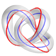
Figure 1: The isosurface of $\phi_{3}=-0.5$ for the local energy minimum at $\kappa=\eta=10$. The solid curve inside the isosurface is the soliton core and the other solid curve is another preimage, namely $\phi^{-1}(-0.87,0,-0.5)$.

IV Results

We have investigated the properties of stable solutions in the modified Ginzburg-Landau model for $H\in[1,7]$. All numerical results have been obtained in a standardized lattice with $360^{3}$ lattice points and lattice constant $h=1/12$. Since this is different from the lattice of Jäykkä (2009), we also recomputed the $H=1$ case in the new standard lattice in order to be able to compare the results for all values of $H$. Some checks were made in lattices of $480^{3}$, $h=1/12$ and $180^{3}$, $h=1/6$ as well.

We chose to investigate the solutions (stable or otherwise) for each $H$ along two lines: $\kappa=10$ and $\eta=10$. As expected, for both lines, we find that there is a limiting value of $\kappa$ ($\eta$) below which no stable solutions can be found. These values depend on $H$. For $H=1$ our results are in agreement with Ward (2002); Jäykkä (2009) and stable solutions are also found for all investigated $H>1$.

This procedure gives us two points on the stable/unstable boundary investigated in Jäykkä (2009), and also information about how the stable solutions change with changing $\kappa$ and $\eta$, which is not so easy to discern from solutions following the actual stable/unstable boundary, where both $\kappa$ and $\eta$ are changing.

IV.1 Error considerations

Derrick’s theorem Derrick (1964) implies that for any static solution of the field equations which is stable against uniform scaling of space, a virial theorem must hold. In this case, it takes the form $E_{B}=E_{K}+E_{W}+3E_{P}$. Obviously, for a numerical approximation, the equation will only be satisfied to within some tolerance. This tolerance would ideally be deduced from the discretization errors, effects of a finite computational domain and the tolerance used to determine convergence, but this seems an insurmountable task. Instead, we have computed the same solution with different lattices (varying both size and density) to give us an estimate of the accuracy. This then gives us an idea of the tolerance in the virial theorem which is achievable at a given lattice. We use this tolerance to estimate the errors in the results.

Apart from error estimates for each simulation, it is important to note what this procedure tells about our results in general. Fig. 2 depicts the energies and core lengths of the $H=7$ simulations for $\kappa=10$ (panel 2a) and for $\eta=10$ (panel 2b) with two different lattice sizes. As can be seen, the differences are minimal apart from the lowest values of $\eta$, where the energy drops significantly faster in the smaller lattice. The difference in the soliton itself is not easily seen until $\eta=0.05$, where we only find a stable soliton in the larger lattice. This is due to the boundaries exerting pressure on the growing (as $\eta$ decreases) soliton, thus destabilizing it.

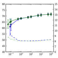
(a)

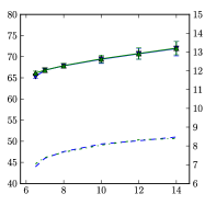
(b)

Figure 2: Total energy and its error limits in normal size and large grid for charge $Q=7$ trefoil. Triangles pointing down (solid blue curve) represents $360^{3}$ and triangles pointing up (solid green) $480^{3}$ lattice, dashed (blue) line the core length in first case and dash-dotted (green) in second case. Energy values are on the left and core length values on the right $y$-axis.

The same effect is present at increasing $\kappa$, but here it cannot destabilize the soliton since increasing $\kappa$ takes us towards a more Faddeev-Skyrme -like system, where the soliton is stable. The effect, however, is large enough to give rise to fast decrease in accuracy. This decrease is the reason for the disparity on the ranges covered: $\eta\in[0.05,1000]$ and $\kappa\in[6,14]$ in this work.

As noted in Section III, the errors in the core length estimates are negligible as long as the core is relatively smooth.

IV.2 Soliton energy

Let us now describe in detail the effects of varying the two parameters on the soliton solutions. First, it should be noted that the energies of the solitons follow the same $E\propto H^{3/4}$ as those of the Faddeev-Skyrme model. Therefore, in what follows, we always normalize the energy: $E\rightarrow E/H^{3/4}$.

Because of the asymptotic limit (5), one expects the energies of the solitons to approach the limit set by the solitons of the Faddeev-Skyrme model as $\kappa,\eta\to\infty$. This expectation is found to be true: for each value of the Hopf invariant at small values of $\kappa$ or $\eta$, the energy is well below the limit and starts growing towards the value of the Faddeev-Skyrme model when either of the parameters is increased, as seen in Figure 3, where we plot the energies of all the identified local minima for all investigated values of $H$ as a function of $\eta$ (panel 3a) and $\kappa$ (panel 3b).

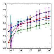
(a)

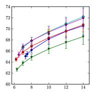
(b)

Figure 3: Plots of the normalized energies ($E/H^{3/4}$) of the minimizers for each $H=1$ (blue circle), $H=2$ (green triangle), $H=3$ (red square), $H=4$ (cyan diamond) and $H=7$ (magenta pentagon). We also include a single data point for $H=5$ (yellow cross) and $H=6$ (black plus).

It is worth noting at this point that our program seems to systematically slightly overestimate the energy: for $H=4$, our values at $\kappa=14,\eta=10$ and $\kappa=10,\eta=1000$ are about $5\%$ above those reported for the Faddeev-Skyrme model Sutcliffe (2007), where an underestimate of about $1\%$ was reported. We believe that since our results show a clear approach towards an asymptotic value, this is an acceptable accuracy for such a simple differentiation scheme as used here. The accuracy could be improved by simply using smaller lattice spacings, but that seems unnecessary for the purposes of this work and would be computationally too expensive for such a large number of simulations.

We also note that at values of $\eta=10,\kappa\geq 10$ and $\eta\geq 10,\kappa=10$, the order of the normalized energies is the same as in the Faddeev-Skyrme model Battye and Sutcliffe (1999); Sutcliffe (2007); Hietarinta and Salo (1999, 2000), further emphasizing the close relationship of the models. It is interesting to note, that the same order also appears in the extended Faddeev-Skyrme model Ferreira et al. (2009). We include two extra data points at $\kappa=\eta=10$ for $H=5,6$ to further demonstrate this. No other simulations were done at $H=5,6$. At lower values of the $\eta$, the order changes, but simultaneously the error bars grow significantly. For small $\kappa$ the order would seem to persist, but this is not the case: the boundary of the region of stable solitons is reached at different values of $\kappa$ for different values of $H$; for example, as $H=1$ reaches the boundary before $H=2$ it will necessarily have lower energy below some limiting value of $\kappa$, thus disrupting the order as is explicitly seen to occur for small $\eta$.

We want to emphasize the fact that the boundary we discover is a bound on the values of $\kappa,\eta$ above which stable solitons can be found. There is no evidence of their existence below the boundary, but it cannot be ruled out using our methods. Also, even for our methods, the bound can be pushed slightly downwards by using more accurate lattices, but instability still eventually occurs (up to what is computationally feasible) as seen for $H=1$ in Jäykkä (2009).

IV.3 Soliton core length

Next, we turn to the length of the soliton core, i.e. the length of the curve $\phi^{-1}(0,0,-1)\in\mathsf{S}^{3}\operatorname{\cong}\mathbb{R}^{3}\operatorname{\cup}\{\infty\}$.

Sutcliffe found that core length for Faddeev-Skyrme Hopfions follow curve $\gamma H^{3/4}$ where his data was fitted to the curve to produce value $\gamma=7.86$ Sutcliffe (2007). We plot the core lengths of our soliton solutions in Figure 4. It is immediately obvious from panel 4b that the solitons collapse to zero size as $\kappa\to 0$ and as $\kappa$ grows, the soliton sizes approach some asymptotic values.. The behavior of the core length is more complex in panel 4a, where $\kappa$ is held constant. Here the core lengths increase, seemingly without limit, as $\eta$ decreases, but do not seem to behave monotonically. However, even though the method used to determine the core length from the computational data is extremely accurate, this gives no information as to how accurately the numerical core approximates its continuum counterpart. The seemingly increasing size of the core for large values of $\eta$ falls within the estimated accuracy of the program, so it can very well be a numerical artifact. A further evidence in favor of this was received by an additional simulation performed for $H=4,\kappa=10,\eta=10000$, which gives very slightly shorter core length as $H=4,\kappa=10,\eta=1000$.

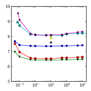
(a)

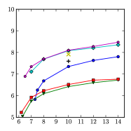
(b)

Figure 4: Plots of the normalized core lengths ($C/H^{3/4}$) of the minimizers for each $H=1$ (blue circle), $H=2$ (green triangle), $H=3$ (red square), $H=4$ (cyan diamond) and $H=7$ (magenta pentagon). We also include a single data point for $H=5$ (yellow cross) and $H=6$ (black plus).

We note that, again, our calculation gives slightly larger values than those reported for the Faddeev-Skyrme Hopfion in Sutcliffe (2007). However, this falls well within the estimated accuracy of the program and the results show a clear approach towards a limiting value, which is more important than the exact value of that limit.

Because every studied soliton follows the same pattern of decreasing core length with decreasing $\kappa$, and increasing core length with decreasing $\eta$, we conjecture that this is a general feature of this model: for core length $C$ one has $\forall H\in\mathbb{Z}:\;\lim_{\eta\to 0}C(H)=\infty$ and $\lim_{\kappa\to 0}C(H)=0$. If this is true, it raises a tantalizing possibility: start with a Faddeev-Skyrme model Hopfion and then begin decreasing $\kappa$ and $\eta$ in such a way that the collapsing and exploding effect of their reduction balance. It is unclear whether such a procedure is possible, but if it is, will it give a stable Hopfion at the limit $\kappa=\eta=0$? That is, a Hopf soliton in pure Ginzburg-Landau model. If such a soliton can be constructed, it seems to require an exact balance between the growing and shrinking effects of decreasing $\eta$ and $\kappa$, and as such, is probably not possible numerically.

IV.4 Region supporting stable solitons

The stable/unstable border is very difficult to analyze because the existence of nontrivial local solutions depends on the topological invariant, $\kappa$ and $\eta$, and their detection depends on the initial state. When the starting point of a simulation is an old solution instead of the configuration (6) and (7), the stability of the simulation also depends on how much $\kappa$ (or $\eta$) is changed from the values used to produce the starting point.

This is best illustrated with charge $Q=4$ solutions. The minimizers obtained from an initial configuration (6) using parameters $p=1$ and $q=4$ have a completely different shape than those obtained from $p=q=2$. They also have consistently higher final energies, but we were able to find stable solutions for smaller values of $\kappa,\eta$ with the first choice of parameters. This reflects on the fact observed by Sutcliffe Sutcliffe (2007) that the number of local minima for the Faddeev-Skyrme model increases with increasing $H$. It appears the same occurs in the present model as well. It is interesting to note, that the most stable soliton is not always the one with the lowest energy.

In order to better understand the relationship between the two models, it would be interesting to see, for each value of $H$, which one of the known Hopfions of the Faddeev-Skyrme model is most stable in the present model. Our single datapoint in this would imply that higher value of $E/C$ would sometimes provide a more stable soliton: the configuration $p,q=1,4$ has higher $E/C$ and can be followed to a lower value of $\kappa$ than $p,q=2,2$. This would give positive support to the conjecture by Babaev that solitons with longer cores would be more stable Babaev (2009).

V Conclusions

We have studied the modification of Ginzburg-Landau model proposed by Ward Ward (2002). We find that the stable solitons exist for all values of the Hopf invariant $H$ up to at least $H=7$, but, just like in the situations studied earlier Ward (2002); Jäykkä (2009), this is only possible when the values of the parameters $\kappa$ and $\eta$ are large enough, and for smaller values, the solitons become unstable against Derrick-type scaling.

The results suggest a conjecture that in this model, the solitons collapse as $\kappa\to 0$, but expand without limit as $\eta\to 0$. It remains an open question, whether these effects could be used to precisely balanced each other and provide a way of constructing a stable knot soliton in the pure Ginzburg-Landau model by starting from a known knot soliton at the Faddeev-Skyrme limit and reducing the two parameters until $\kappa=0$.

We gain further insight into the relationship between the Ginzburg-Landau and Faddeev-Skyrme models, by noting that the order of the values of the normalized energies at different values of the Hopf invariant is the same as in the Faddeev-Skyrme model Battye and Sutcliffe (1999); Sutcliffe (2007); Hietarinta and Salo (1999, 2000) and extended Faddeev-Skyrme model Ferreira et al. (2009). The fact that in the modified Ginzburg-Landau model the solitons are local minima, not global as in the Faddeev-Skyrme model, is interesting from condensed matter physics point of view, where local minima are often of great importance.