Matrix completion with column manipulation: Near-optimal sample-robustness-rank tradeoffs

Abstract

This paper considers the problem of matrix completion when some number of the columns are completely and arbitrarily corrupted, potentially by a malicious adversary. It is well-known that standard algorithms for matrix completion can return arbitrarily poor results, if even a single column is corrupted. One direct application comes from robust collaborative filtering. Here, some number of users are so-called manipulators who try to skew the predictions of the algorithm by calibrating their inputs to the system. In this paper, we develop an efficient algorithm for this problem based on a combination of a trimming procedure and a convex program that minimizes the nuclear norm and the $\ell_{1,2}$ norm. Our theoretical results show that given a vanishing fraction of observed entries, it is nevertheless possible to complete the underlying matrix even when the number of corrupted columns grows. Significantly, our results hold without any assumptions on the locations or values of the observed entries of the manipulated columns. Moreover, we show by an information-theoretic argument that our guarantees are nearly optimal in terms of the fraction of sampled entries on the authentic columns, the fraction of corrupted columns, and the rank of the underlying matrix. Our results therefore sharply characterize the tradeoffs between sample, robustness and rank in matrix completion.

1 Introduction

Previous work in low-rank matrix completion [10, 11, 19, 15] has demonstrated the following remarkable fact: given a $m\times n$ matrix of rank $r$, if its entries are sampled uniformly at random, then with high probability, the solution to a convex and in particular tractable optimization problem yields exact reconstruction of the matrix when only $O((m+n)r\log(m+n))$ entries are sampled.

Yet as our simulations demonstrate, if even a few columns of this matrix are corrupted, the output of these algorithms can be arbitrarily skewed from the true matrix. This problem is particularly relevant in so-called collaborative filtering, or recommender systems. Here, based on only partial observation of users’ preferences, one tries to obtain accurate predictions for their unrevealed preferences. It is well known and well documented [29, 47] that such recommender systems are susceptible to manipulation by malicious users who can calibrate all their inputs adversarially. It is of great interest to develop efficiently scalable algorithms that can successfully predict preferences of the honest users based on the corrupted and partially observed data, while identifying the manipulators.

The presence of partial observation and potentially adversarial input makes a priori identification of corrupted column versus good column a challenging task. For example, a simple method that works fairly well under full observation and purely random corruption, is to use the correlation between the columns. Since the authentic columns of a low-rank matrix are linearly correlated, under suitable conditions they can be identified as those which have a high correlation with many other columns. However, when partial observations are present, this method fails since it is not immediately clear even how to compute the correlation—most pairs of columns do not share an observed coordinate—let alone finding the corrupted columns which can disguise themselves to look like a partially observed authentic column. At first sight, it is unclear how to accomplish the two tasks simultaneously: completing unobserved entries, and identifying corrupted columns.

This paper studies this precise problem. We do so by exploiting the algebraic structure of the problem: the non-corrupted columns form a low-rank matrix, while the corrupted columns can be seen as a column-sparse matrix. Thus, the mathematical problem we address is to decompose a low-rank matrix from a column-sparse matrix, based on only partial observation. Specifically, suppose we are given partial observation of a matrix $M$, which can be written as

$$M=L_{0}+C_{0},$$ (1)

where $L_{0}$ is low-rank and $C_{0}$ has only a few non-zero columns. Here the entries of $C_{0}$ may have arbitrary magnitude and can even be adversarially built; the column/row space of $L_{0}$ as well as the positions of non-zero columns of $C_{0}$ are unknown. With a subset of the entries of $M$ observed, can we efficiently recover $L_{0}$ on the non-corrupted columns, and also identify the non-zero columns of $C_{0}$? And, how do the rank and the number of corrupted columns impact the number of observations needed?

We provide an affirmative answer to the first question, and a quantitative solution to the second. In particular, we develop an efficient algorithm, which is based on a trimming procedure followed by a convex program that minimizes the nuclear norm and the $\ell_{1,2}$ norm. We provide sufficient conditions under which this algorithm provably recovers $L_{0}$ and identifies the corrupted columns. Our algorithm succeeds even when a vanishing fraction of randomly located entries are observed and a significant fraction of the columns are corrupted; moreover, the number of observations we need depends near optimally, in an information-theoretic sense, on the rank of $L_{0}$ and the number of corrupted columns. Significantly, we do not assume anything about the values nor the locations of observations on the corrupted columns.

We note that our corruption model is very general. By making no assumption on the corrupted columns, our results cover, but are not limited to, adversarial manipulation. For example, the corrupted columns can also represent persistent noise and abnormal sub-populations that are not well modeled by a (known) probabilistic model. We discuss several such examples in Section 1.1.

Conceptually, our results establish the relation and tradeoffs between three aspects of the problem: sample complexity (the number of observed entries), model complexity (the rank of the matrix) and adversary robustness (the number of arbitrarily corrupted columns). While the interplay between sample and model complexities is a recurring theme in modern work of statistics and machine learning, their relation with robustness (particularly to arbitrary and adversarial corruption, as opposed to neutral, stochastic noise) seems much less well understood. Our results show that with more samples, one can not only estimate matrices of higher rank, but also be robust to more adversarial columns. Importantly, we provide both (and nearly matching) upper and lower bounds, thus establishing a complete and sharp characterization of this phenomenon. To establish lower bounds under arbitrary corruption, we use techniques that are quite different from existing ones for stochastic corruption that largely rely on Fano’s inequality and the alike.

Paper Organization

We postpone the discussion of related work to Section 3 after we state our main theorems. In Section 1.1 we describe several application motivating our study, followed by a summary of our main technical contributions in Section 1.2. In Section 2 we give the mathematical setup of the robust matrix completion problem with corrupted columns. In Section 3 we provide the main results of the paper: a robust matrix completion algorithm, a sufficient condition for the success of the algorithm, and a matching inverse theorem showing the optimality of the algorithm. We also survey relevant work in the literature and discuss their connection to our results. In Section 4 we discuss implementation issues and provide empirical results. We prove the two main theorems in Sections 5 and 6, respectively, with some of the technical details deferred to the appendix. The paper concludes with a discussion in Section 7.

1.1 Motivating Applications

Our investigation is motivated by several important problems in machine learning and statistics, which we discuss below.

Manipulation-Robust Collaborative Filtering

In online commerce and advertisement, companies collect user ratings for products, and would like to predict user preferences based on these incomplete ratings—a problem known as collaborative filtering (CF). There is a large and growing literature on CF; most well-known is the work on the Netflix prize [4], but also see [1, 45] and the references therein. Various CF algorithms have been developed [20, 35, 40, 39, 44]. A typical approach to cast it as a matrix completion problem: the preferences across users are known to be correlated and thus modeled as a low-rank matrix $L_{0}$, and the goal is to estimate $L_{0}$ from its partially observed entries. However, the quality of prediction may be seriously hampered by (even a small number of) manipulators—potentially malicious users, who calibrate (possibly in a coordinated way) their ratings and the entries they choose to rank in an attempt to skew predictions [47, 29]. In the matrix completion framework, this corresponds to the setting where some of the columns of the observed matrix are provided by manipulative users. As the ratings of the authentic users correspond to a low-rank matrix $L_{0}$, the corrupted ratings correspond to a column-sparse matrix $C_{0}$. Therefore, in order to perform collaborative filtering with robustness to manipulation, we need to identify the non-zero columns of $C_{0}$ and at the same time recover $L_{0}$, given only a set of incomplete entries. This falls precisely into the scope of our problem.

Robust PCA

In the robust Principal Component Analysis (PCA) problem [48, 50, 32, 38], one is given a data matrix $M$, of which most of the columns correspond to authentic data points that lie in a low-dimensional space—the space of principal components. The remaining columns are outliers, which are not (known to be) captured by a low-dimensional linear model. The goal is to negate the effect of outliers and recover the true +principal components. In many situations such as problems in medical research (see e.g., [12]), there are unobserved variables/attributes for each data point. The problem of robust PCA with partial observation—recovering the principal components in the face of partially observed samples and also corrupted points—falls directly into our framework.

Crowdsourcing

Crowdsourcing has emerged as a popular approach for using human power to solve learning problems. Here multiple-choice questions are distributed to several workers, whose answers are then collected and aggregated in an attempt to obtain an accurate answer to each question. In a simplified setting called the Hammer-Spammer model [24, 25], a worker is either a hammer who gives correct answers, or a spammer who answers completely randomly. A more general setting is considered in [26], where the spammers need not follow a probabilistic model and may submit any answers they want, for instance with an unknown bias, or even adversarially. This problem can be mapped to our matrix framework, where rows correspond to questions and columns to workers, with $L_{0}$ representing the matrix of true answers from the hammers and $C_{0}$ the answers from the spammers. Each worker typically answers only a subset of the questions, leading to partial observation.

Model Mismatch

More generally, the corrupted columns can encompass any observations that are not captured by the assumed low-rank model. These observations may be generated from an unknown population or affected by factors beyond the knowledge of the modeler, but not necessarily adversarial. Such mismatch between the models and data is ubiquitous. For instance, in collaborative filtering there may exist a small set of atypical users whose preferences are very weakly correlated with the majority and thus difficult to infer using data from the majority. In PCA some data points may simply not conform to the low-dimensional linear model. The answers from some workers in crowdsourcing systems may be erroneous as the data collecting process is non-ideal and not fully controllable. It is difficult to accurately model or recover these columns, but our results guarantee that they do not hinder the recovery of the other columns.

1.2 Main Contributions

In this paper, we propose a new algorithm for matrix completion in the presence of corrupted columns and provide performance guarantees. Specifically, we have the following results:

1. We develop a two-step matrix completion algorithm, which first trims the over-sampled columns of the matrix, and then solves a convex optimization problem involving the nuclear norm and the $\ell_{1,2}$ norm. Our algorithm extends the standard nuclear norm minimization approach for matrix completion, and the use of trimming and the $\ell_{1,2}$ norm plays a crucial role in achieving robustness to arbitrary column-wise corruption.

2. For an $n\times n$ incoherent matrix with rank $r$ and a subset of its columns arbitrarily corrupted, we show that if a fraction of $p$ randomly located entries are observed in the uncorrupted columns, then our algorithm provably identifies the corrupted columns and completes the uncorrupted ones as long as $p$ obeys the usual condition $p\gtrsim\frac{r\log^{2}n}{n}$ for matrix completion, and in addition the fraction $\gamma$ of corrupted columns satisfies $\gamma\lesssim\frac{p}{r\sqrt{r}\log^{3}n}$.

3. We further show that the two conditions are near-optimal, in the sense that if $p\lesssim\frac{r\log n}{n}$ or $\gamma\gtrsim\frac{p}{r}$, then an adversary can corrupt the columns in such a way that all algorithms fail with probability bounded away from zero. Therefore, our results establish tight bounds for the sample-robustness-rank tradeoffs in matrix completion.

4. We develop a variant of the Augmented Lagrangian Multipliers (ALM) method for solving the convex optimization problem in our algorithm. Empirical results on synthetic data are provided, which corroborate with our theoretical findings and show that our algorithm is more robust than standard matrix completion algorithms.

2 Problem Setup

Suppose $M$ is a ground-truth matrix in $\mathbb{R}^{m\times(n+n_{c})}$. Among the $n+n_{c}$ columns of $M$, $n$ of them (we will call them authentic or non-corrupted) span an $r$-dimensional subspace of $\mathbb{R}^{m}$, and the remaining $n_{c}$ columns are arbitrary (we will call them corrupted). We only observe a subset of the entries of the matrix $M$, and the goal is to infer the true subspace of the authentic columns and the identities of the corrupted ones.

Under the above setup, it is clear that the matrix $M$ can be decomposed as $M=L_{0}+C_{0}.$ Here $L_{0}\in\mathbb{R}^{m\times(n+n_{c})}$ is the matrix containing the authentic columns, and therefore $\text{rank}(L_{0})=r$. The matrix $C_{0}\in\mathbb{R}^{m\times(n+n_{c})}$ contains the corrupted columns, so at most $n_{c}$ of the columns of $C_{0}$ are non-zero. Let $I_{0}\subset[n+n_{c}]$ be the indices of the corrupted columns; that is, $I_{0}:=\text{column-support}(C_{0}),$ where $\left|I_{0}\right|=n_{c}$. Let $\Omega\subseteq[m]\times[n+n_{c}]$ be the set of indices of the observed entries of $M$, and $\mathcal{P}_{\Omega}$ the projection onto the matrices supported on $\Omega$, which is given by

$$\left(\mathcal{P}_{\Omega}X\right)_{ij}=\begin{cases}X_{ij},&\quad(i,j)\in\Omega,\\ 0,&\quad(i,j)\notin\Omega.\end{cases}$$

With this notation, our goal is to exactly recover from $\mathcal{P}_{\Omega}M$ the authentic columns in $L_{0}$ and the corresponding column space as well as the locations $I_{0}$ of the non-zero columns of $C_{0}$.

2.1 Assumptions

In general, it is not always possible to complete a low-rank matrix in the presence of corrupted columns. For example, if $L_{0}$ has only one non-zero column, it is impossible to distinguish $L_{0}$ from $C_{0}$ even when $M$ is fully observed. It is also well-known in the matrix completion literature [10, 19, 27] that if $L_{0}$ has only one non-zero row, or if one row or column of $L_{0}$ is completely unobserved, then asking to recover $L_{0}$ from partial observations is problematic. To avoid these pathological situations, we will assume that $L_{0}$ satisfy the now standard incoherence condition [10] and the observed entries on the authentic columns of $L_{0}$ are sampled at random. We note that we make no assumptions on the values or locations of the observed entries of corrupted columns in $C_{0}$.

2.1.1 Incoherence Condition

Suppose $L_{0}$ has the Singular Value Decomposition (SVD) $L_{0}=U_{0}\Sigma_{0}V_{0}^{\top}$, where $U_{0}\in\mathbb{R}^{m\times r}$, $V_{0}\in\mathbb{R}^{(n+n_{c})\times r}$ and $\Sigma_{0}\in\mathbb{R}^{r\times r}$. We use $\left\|\cdot\right\|_{2}$ to denote the vector $\ell_{2}$ norm, and $e_{i}$ be the $i$-th standard basis vector whose dimension will be clear in context.

Assumption 1 (Incoherence).

The matrix $L_{0}$ is zero on the columns in $I_{0}$. Moreover, $L_{0}$ satisfies the following two incoherence conditions with parameter $\mu$:

$$\max_{1\leq i\leq m}\left\|U_{0}^{\top}e_{i}\right\|_{2}^{2} \leq\mu\frac{r}{m},$$

$$\max_{1\leq j\leq n+n_{c}}\left\|V_{0}^{\top}e_{j}\right\|_{2}^{2} \leq\mu\frac{r}{n}.$$

Since the columns of $L_{0}$ in $I_{0}$ are superposed with the arbitrary $C_{0}$, there is no hope of recovering these columns. Therefore, there is no loss of generality to assume $L_{0}$ is zero on $I_{0}$. Consequently, the matrix $V_{0}^{\top}$ has at most $n$ non-zero columns (all in $I_{0}^{c}$), and accordingly the denominator on the right hand side of the second inequality above is $n$ instead of the full dimension $n+n_{c}$.

The two incoherence conditions are needed for completion of $L_{0}$ from partial observations even with no corrupted columns. The incoherence parameter $\mu$ is known to be small in various natural models and applications [10, 11]. The second inequality in Assumption 1 is necessary in the presence of corrupted columns, even when the matrix is fully observed. This inequality essentially enforces that the information about the column space of $L_{0}$ is spread out among the columns. If, for instance, an authentic column of $L_{0}$ were not in the span of all the other columns, one could not hope to distinguish it from a corrupted column (cf. [50]).

Finally, we note that previous work on matrix completion often imposes a strong incoherence condition $\max_{i,j}\left|\left(U_{0}V_{0}^{\top}\right)_{ij}\right|\leq\sqrt{\frac{\mu r}{mn}}$ [10, 11, 19, 42]. We do not need this assumption, thus improving over these previous results. Further discussion on this point is provided after our main theorems.

2.1.2 Sampling Model

Recall that $I_{0}$ is the indices of the corrupted columns. Let $\tilde{\Omega}:=\Omega\cap\left([m]\times I_{0}^{c}\right)$ be the set of indices of observed entries on the non-corrupted columns. We use the following definition.

Definition 1 (Bernoulli model).

Suppose $\Theta_{0}\subseteq[m]\times[n+n_{c}]$. A set $\Theta$ is said to be sampled from the Bernoulli model with probabilities $\left\{p_{j}\right\}_{j=1}^{n+n_{c}}$ on $\Theta_{0}$ if each element $(i,j)$ of $\Theta_{0}$ is contained in $\Theta$ with probability $p_{j}$, independently of all others. If $p_{j}=p$ for $j$, then $\Theta$ is said to be sampled from the Bernoulli model on $\Theta_{0}$ with uniform probability $p$.

We can now specify our assumption on how the observed entries are sampled.

Assumption 2 (Sampling).

The set $\tilde{\Omega}$ is sampled from the Bernoulli model with probabilities $\{p_{j}\}$ on $[m]\times I_{0}^{c}$, where $p_{j}\geq p$ for all $j\in I_{0}^{c}$. Moreover, $\tilde{\Omega}$ is independent of $\mathcal{P}_{\Omega}C_{0}$, the observed entries on the corrupted columns.

Note that our model is more general than the uniform sampling model assumed in some previous work—we only require a lower bound on the observation probabilities of the non-corrupted columns, so some columns may have an observation probability higher than $p$. Importantly, the Bernoulli model is not imposed on the corrupted columns. The adversary may choose to reveal all entries on columns in $I_{0}$ or just a fraction of them, and the locations of these observed entries may be chosen randomly or adversarially depending on $L_{0}$. The assumption of $\tilde{\Omega}$ being independent of the corrupted columns is needed for technical reasons. We conjecture that it is only an artifact of our analysis and not actually necessary, as indicated by our empirical results.

2.1.3 Corrupted Columns

Let $\gamma:=\frac{n_{c}}{n}$ be the ratio of the number of corrupted columns to the number of authentic columns. Other than the independence requirement above, we make no assumption whatsoever on the corrupted columns in $C_{0}$. The incoherence assumption is imposed on the authentic $L_{0}$, not on $M$ or $C_{0}$, as is the sampling assumption, and therefore the corrupted columns are not restricted in any way by these. These columns need not follow any probabilistic distributions, and they may be chosen by some adversary who aims to skew one’s inference of the non-corrupted columns. One consequence of this is that we will not be able to recover the values of the completely corrupted columns of $C_{0}$, but we are able to reveal their identities.

3 Main Results: Algorithms, Guarantees and Limits

The main result of this paper says that despite the corrupted columns and partial observation, we can simultaneously recover $L_{0}$, the non-corrupted columns, and identify $I_{0}$, the position of the corrupted columns, as long as the number of corrupted columns and unobserved entries are controlled. Moreover, this can be achieved efficiently via a tractable procedure, given as Algorithm 1.

Algorithm 1 Manipulator Pursuit

Input: $\mathcal{P}_{\Omega}(M)$,$\Omega$,$\lambda$, $\rho$.

Trimming: For $j=1,\ldots,n+n_{c}$, if the number of observed entries $h_{j}$ on the $j$-th column satisfies $h_{j}>\rho m$, then randomly select $\rho m$ entries (by sampling without replacement) from these $h_{j}$ entries and set the rest as unobserved. Let $\hat{\Omega}$ be the set of remaining observed indices.

Solve for optimum $(L^{\ast}$, $C^{\ast}$):

$$\textrm{minimize}_{L,C} \left\|L\right\|_{\ast}+\lambda\left\|C\right\|_{1,2}$$ (2)

subject to $$\mathcal{P}_{\hat{\Omega}}(L+C)=\mathcal{P}_{\hat{\Omega}}(M)$$

Set $I^{*}=\text{column-support}\left(C^{*}\right):=\{j:\;C_{ij}^{\ast}\neq 0\text{ for some }i\}$.

Output: $L^{*}$, $C^{*}$ and $I^{*}$.

The algorithm has two steps. In the first trimming step, we find columns with a large number of observed entries, and throw away some of these entries randomly. This step is important, both in theory and empirically, to achieve good performance: an adversary may choose to reveal (and corrupt) a large number of entries on certain columns, which may skew the next step of the algorithm; the trimming step protects against this effect. Note that we cannot directly identify these over-sampled corrupted columns by counting the number of observations—under the (non-uniform) sampling model in Assumption 2, some authentic columns are also allowed to have many observed entries.

In the next step of the algorithm, we solve a convex program with the trimmed observations as the input. The convex program, in fact a Semidefinite Program (SDP), finds a pair $(L^{*},C^{*})$ that is consistent with the observations and minimizes the weighted sum of the nuclear norm $\left\|L\right\|_{*}$ and the matrix $\ell_{1,2}$ norm $\left\|C\right\|_{1,2}$, where $\left\|L\right\|_{*}$ is the sum of singular values of $L$ and a convex surrogate of its rank, and $\left\|C\right\|_{1,2}$ is the sum of the column $\ell_{2}$ norms of $C$ and a convex surrogate of its column sparsity. The algorithm has two parameters: the threshold $0<\rho<1$ for trimming and the coefficient $\lambda>0$ for the weighted sum in the convex program. Our theoretical results specify how to choose their values.

We say Algorithm 1 succeeds if we have $\mathcal{P}_{U_{0}}(L^{*})=L^{*}$, $\mathcal{P}_{I_{0}^{c}}(L^{*})=L_{0}$ and $I^{*}\subseteq I_{0}$ for any optimal solution $(L^{*},C^{*})$ of (2), where $\mathcal{P}_{U_{0}}(L^{*}):=U_{0}U_{0}^{\top}L^{*}$ is the projection of the columns of $L^{*}$ onto the column space of $L_{0}$, and $\mathcal{P}_{I_{0}^{c}}(L^{*})$ is the projection of $L^{*}$ onto the matrices supported on the column indices in $I_{0}^{c}$, given by

$$\left[\mathcal{P}_{I_{0}^{c}}(L^{*})\right]_{ij}=\begin{cases}L^{*}_{ij},&\text{if }j\not\in I_{0},\\ 0,&\text{if }j\in I_{0}.\end{cases}$$

That is, the algorithm succeeds we recover the true column space of the original $L_{0}$ and complete its uncorrupted columns, and at the same time identify the locations of the corrupted columns. Note that the definition of success allows for $I^{*}\subsetneq I_{0}$. In this case it may appear that some corrupted columns are unidentified and included in $L^{*}$, but it is actually not a problem: the requirement $\mathcal{P}_{U_{0}}(L^{*})=L^{*}$ means that these unidentified “corrupted” columns can be completed to lie in the true column space of $L_{0}$, so they are essentially not corrupted, as they are indistinguishable from a partially observed authentic column and do not affect the completion.

3.1 Sufficient Conditions for Recovery

Our first main theorem guarantees that under some natural conditions, our algorithm exactly recovers the non-corrupted columns and the identities of the corrupted columns with high probability. Recall that $p$ is a lower bound of the observation probability on the non-corrupted columns, $\gamma:=\frac{n_{c}}{n}$ the ratio between the numbers of corrupted and uncorrupted columns, and $\rho$ the trimming threshold.

Theorem 1.

Let $\alpha:=\frac{\rho}{p}$. There exist universal positive constant $c_{1}$ and $c_{2}$ for which the following holds. Suppose the Assumptions 1 and 2 hold. If in Algorithm 1 we take

$$\lambda\in\left[\sqrt{\left(1+\frac{1}{\alpha}\right)\frac{\mu r\log(m+n)}{pn}},\frac{1}{48\sqrt{\sqrt{(1+\alpha)\mu r}\gamma n\log(m+n)}}\right],$$

and $(p,\gamma)$ satisfies

$$p \geq c_{1}\left(1+\frac{1}{\alpha}\right)\frac{\mu r\log^{2}(m+n)}{\min(m,n)},$$ (3)

$$\gamma \leq c_{2}\frac{\alpha}{1+\alpha\sqrt{\alpha}}\frac{p}{\mu r\sqrt{\mu r}\log^{3}(m+n)},$$ (4)

then Algorithm 1 succeeds with probability at least $1-20(m+n)^{-5}$. Note that the interval for $\lambda$ is non-empty under the condition (4).

We prove this theorem in Section 5.

The two conditions (3) and (4) have the natural interpretation that the algorithm succeeds as long as there is sufficiently many observed entries (in particular, more than the degrees of freedom of a rank-$r$ matrix), and the number of corrupted columns is not too large relative to the number of observed entries. We discuss these two conditions in more details in the next sub-section. The theorem also shows that the parameter $\lambda$ in the convex program (2) can take any value in a certain range.

3.1.1 Consequences

We explore several consequences of Theorem 1. The conditions (3) and (4) above involve the value of the parameter $\rho$ from trimming in Algorithm 1. The conditions become the least restrictive if $\alpha:=\frac{\rho}{p}=\Theta(1)$, i.e., when $\rho$ is of the same order of $p$. Choosing $\rho$ optimally in this way gives the following corollary.

Corollary 1 (Optimal Bound).

There exist universal constant $c_{1}$ and $c_{2}$ such that the following holds. Suppose the Assumptions 1 and 2 hold, and we take $\rho=p$ and $\lambda=\sqrt{\frac{2\mu r\log(m+n)}{pn}}$ in Algorithm 1. Algorithm 1 succeeds with probability at least $1-20(m+n)^{-5}$ as long as $(p,\gamma)$ satisfy (3) and (4) with $\alpha=1$.

For a more concrete example, suppose the observation probability satisfies $p\gtrsim\frac{\sqrt{\mu^{3}r^{3}}\log^{3}n}{n^{1-\kappa}}$, then Corollary 1 guarantees success of our algorithms when the number of corrupted entries $\gamma n$ is less than $n^{\kappa}$.

In a conference version [18] of this paper, we analyze the second step of Algorithm 1 (i.e., without trimming, or equivalently $\rho=1$) and show that it succeeds if $(p,\gamma)$ satisfy (among other things) the condition

$$\gamma\lesssim\frac{p^{2}}{\left(1+\frac{\mu r}{p\sqrt{n}}\right)^{2}\mu^{3}r^{3}\log^{6}(m+n)}.$$

This result is significantly improved by Corollary 1 (in particular, compared to the condition (4) with $\alpha=1$), which allows for an order-wise larger number of corrupted columns. Our analysis reveals that the trimming step in Algorithm 2 is crucial to this improvement.

Remark 1.

In practice, we may estimate the value of $p$ by using a robust mean estimator (e.g., the median or trimmed mean) of the fraction of observed entries over the columns. Given such an estimate $\hat{p}$, we can set $\rho=\hat{p}$ and $\lambda=\sqrt{\frac{c\log(m+n)}{\hat{p}n}}$ for some constant $c$ (say $50$), and the algorithm’s success is guaranteed by Theorem 1 and Corollary 1 for $\mu r=O(1)$. (Note that while we may not know $n$, we do know the value of $n+n_{c}$, which differs from $n$ by at most a factor of $2$ whenever $n_{c}\leq n$.) This approach is taken in our empirical studies in Section 4.

Setting $p=1$ in Corollary 1 immediately yields a guarantee for the full observation setting.

Corollary 2 (Full Observation).

Suppose the Assumptions 1 and 2 hold with $p=1$. If we take $\rho=1$ and $\lambda=\sqrt{\frac{2\mu r\log(m+n)}{n}}$ in Algorithm 1, and $\gamma:=\frac{n_{c}}{n}$ satisfies

$$\gamma \leq c_{1}^{\prime}\frac{1}{\mu r\sqrt{\mu r}\log^{3}(m+n)}$$

for some universal constant $c_{1}^{\prime}$, then Algorithm 1 succeeds with probability at least $1-20(m+n)^{-5}$.

The full observation setting of our model corresponds to the Robust PCA problem with sample-wise corruption (cf. Section 1.1), which is previously considered in [49, 50]. There they propose an algorithm called Outlier Pursuit, which is similar to the second step of our Algorithm1 and shown to succeed in the full observation setting if $\gamma\lesssim\frac{1}{\mu r}$. Our result in Corollary 2 is off by a small factor of $\sqrt{\mu r}\log^{3}(m+n)$. This sub-optimality can be removed by a more careful analysis in the setting with $p$ close to $1$, but we choose not to delve into it.

On the other hand, setting $\gamma=0$ gives a guarantee for the standard exact matrix completion setting with clean observations. Our result is powerful enough that it in fact improves upon some previous results in this setting.

Corollary 3 (Matrix Completion).

Suppose $\gamma=0$ and the Assumption 1 and 2 hold. If we take $\rho=1$ and $\lambda\geq\sqrt{\frac{2\mu r\log(m+n)}{pn}}$ in Algorithm 1, and $p$ satisfies

$$p\geq c_{1}^{\prime\prime}\frac{\mu r\log^{2}(m+n)}{\min(m,n)}$$

for some universal constant $c_{1}^{\prime\prime}$, then Algorithm 1 succeeds with probability at least $1-20(m+n)^{-5}$.

Exact matrix completion is considered in the seminal work [10] and subsequently in [11, 19, 42], in which the low-rank matrix $L_{0}$ is assumed to satisfied two incoherence conditions: the standard incoherence condition with parameter $\mu$ as in Assumption 1, and an additional strong incoherence condition $\left\|UV\right\|_{\infty}\leq\sqrt{\frac{\mu_{\text{str}}r}{mn}}$. They show that $L_{0}$ can be exactly recovered via nuclear norm minimization if $p\gtrsim\frac{\max\left\{\mu,\mu_{\text{str}}\right\}r\log^{2}(m+n)}{\min\left\{m,n\right\}}$. Corollary 3 improves upon this result by removing the dependence on the strong incoherence parameter $\mu_{\text{str}}$, which can be as large as $\mu r$. This improvement was also observed in the recent work in [15, 16].

We have seen that Theorem 1 and Corollary 1 give, as immediate corollaries, strong bounds for the special cases of full observation and standard matrix completion, which is a testament to the sharpness of our results. In fact, we show in the next sub-section that the conditions in Theorem 1 are near-optimal.

3.2 Information-Theoretic Limits for Recovery

Corollary 1 says that the conditions (3) and (4) with $\alpha=1$ are sufficient for our algorithm to succeed. Theorem 2 below shows that these conditions are in fact close to being information-theoretic (minimax) optimal. That is, they cannot be significantly improved by any algorithm regardless of its computational complexity. Note that the theorem tracks the values of $\mu$, $r$, $p$ and $\gamma$, so all of them can scale in a non-trivial way with respect to $n$.

Theorem 2.

Suppose $m=n\geq 4$, $\mu r\leq\frac{n}{\log(2n)}$, and $(p,\gamma)$ satisfy

$$p \leq\frac{\mu r\log(2n)}{2n}$$ (5)

$$\textbf{ or}\quad\gamma :=\frac{n_{c}}{n}\geq\frac{2p}{\mu r}.$$ (6)

Then any algorithm will fail to output the correct column space with probability at least $\frac{1}{16}$; more precisely, for all measurable functions $\hat{L}$ of $M$ and $\Omega$,

$$\max_{L_{0},C_{0},\Omega\backslash\tilde{\Omega}}\mathbb{P}\left[\mathcal{P}_{U_{0}}(\hat{L})\neq\hat{L}\right]\geq\frac{1}{16},$$

where the maximization ranges over all matrix pairs $(L_{0},C_{0})$ and observed indices on the corrupted columns $\Omega\backslash\tilde{\Omega}$ that satisfy the Assumptions 1 and 2, and the probability is with respect to the distribution of the observed indices on the non-corrupted columns $\tilde{\Omega}$.

We prove this theorem in Section 6.

By comparing with Theorem 2, we see that the conditions in Corollary 1 are close to the achievable limits. In particular, with $\alpha=1$, the condition (3) on $p$ matches (5) up to one logarithmic factor, and the condition (4) on $\gamma$ is worse than (6) by a factor of $c\sqrt{\mu r}\log^{3}n$. In particular, both conditions are optimal up to logarithmic factors in the case of constant rank and incoherence $\mu r=O(1)$. It is of interest to study whether this small gap can be closed, potentially by tightening up the sufficient conditions in Theorem 1 and Corollary 1.

The failure condition (5) is an extension of a standard result for matrix completion in [11, Theorem 1.7]. To gain some intuition on the second condition (6), we consider the case with $\mu r=1$, for which the condition becomes $n_{c}\gtrsim pn$. This means that with probability bounded away from zero, the number of observed corrupted entries in the first row exceeds that of observed authentic entries in the same row. In this case, if the corrupted entries in the other rows are chosen to be consistent with the true column space (on all but the first coordinates), then no algorithm can tell which of the two sets of entries in the first row is actually authentic, and therefore recovery of this row is impossible. Theorem 2 is proved using an extension of the above argument—by demonstrating a particular way of corrupting $n_{c}\gtrsim\frac{pn}{\mu r}$ columns that provably confuses any algorithm.

Implications for Robust PCA:

Recall the Robust PCA setting with full observations ($p=1$) and the Outlier Pursuit algorithm discussed after Corollary 2 in Section 3.1. Theorem 2 shows that $\gamma\gtrsim\frac{1}{\mu r}$ is necessary, so the guarantee for Outlier Pursuit given in [50] is order-wise optimal.

3.3 Sample-Robustness-Rank Tradeoffs

The results in the last two-subsections highlight the tradeoffs between sample complexity, outlier robustness and model complexity (matrix rank). In particular, given a higher the observation probability $p$, one can handle a higher fraction $\gamma$ of corrupted columns and a higher rank $r$ of the underlying matrix. The other direction is also true: with a smaller $p$, the fraction of allowable corrupted columns and the allowable rank will necessarily become smaller, regardless of the algorithm and the amount of computational. Theorems 1 and 2 provide the precise conditions that $p$, $\gamma$ and $r$ need to obey.

We emphasize that here we consider robustness to arbitrary and possibly adversarial corruption. Our results characterize, in terms of both upper and lower bounds, the tradeoffs between adversary robustness and sample/model complexities. This can be put into the context of the study of modern high-dimensional statistics [41, 7], where the relationship between sample and model complexities is a central topic of interest. More recently, a line of work has focused on the tradeoffs between computational complexity and various statistical quantities [13, 5, 36, 53]. Our results can be viewed as adding a new dimension to these recent lines of work: we consider another axis of the problem—robustness (to adversarial corruption)—and its relation to other statistical quantities. Therefore, while we investigate a specific problem (matrix completion), we expect sample-robustness tradeoffs to be relevant in a broader context.

Finally, we note that our empirical study in Section 4 demonstrate the following phenomenon: If we further assume that the corrupted columns are randomly generated and independent of each other, then our algorithm can recover $L_{0}$ from a much higher number $n_{c}$ of corrupted columns than is predicted by Theorems 1 and 2 (which require, among other things, $n_{c}=\gamma n\leq 1$). In particular, the corrupted columns can significantly out-number the authentic columns. This means our algorithm is useful well beyond the adversarial corruption setting considered in the theorems above, and its actual performance can become better if the corruption is more restricted and “benign”. A similar phenomenon is observed in [32, 52] for the special case of full observation. Here we therefore see another level of sample-robustness-rank tradeoffs: If we only ask for a weaker sense of robustness, namely, robustness against randomly corrupted columns as opposed to arbitrary ones, then we have more relaxed requirements on the observation probability, the rank and the number of corrupted columns. It is an interesting open problem to rigorously quantify the interplay between the nature of the corruption and the recovery performance.

3.4 Connections to Prior Work and Innovation

Recent work in matrix completion shows that by using convex optimization [10, 11, 19, 42] or other algorithms [27, 23, 8], one can exactly recover an $n\times n$ rank-$r$ matrix with high probability from as few as $O(nr\mathrm{poly}\log n)$ (clean) entries. Our paper extends this line of work and shows that even if all the observed entries on some columns are completely corrupted (by possibly adversarial noise), one can still recover the non-corrupted columns as well as the identity of the corrupted ones. As discussed before, our work also extends the work in [49, 50], which only considers the full observation setting; see also [2] for results on the full observation setting with noise. The centerpiece of our algorithm is a convex optimization problem that is a convex proxy to a very natural but intractable algorithm for our task, namely, finding a low-rank matrix $L$ and a column-sparse matrix $C$ consistent with the observed data. Such convex surrogates for rank and support functions have been used (often separately) in problems involving low-rank matrices [43, 10]) and in problems with group-sparsity [51, 21]. When this manuscript is under preparation, we learn about the very recent work [28], which also studies robust matrix completion under column-wise sparse corruption, albeit under a somewhat different setting. Their results are focused on the noisy setting with general sampling distributions, but do not guarantee exact recovery in the noiseless case.

Our work is also related to the problem of separating a low-rank matrix and an overall (element-wise) sparse matrix from their sum [9, 14] (this is sometimes called the low-rank-plus-sparse problem, or $L+S$ for short). This problem has also been studied under the partial observation setting [9, 17, 33]. Compared to this line of work, our results indicate that separation is possible even if the low-rank matrix is added with a column sparse matrix instead of an overall sparse matrix. In particular, we allow all the observations from some columns to be completely corrupted. In contrast, existing guarantees for the $L+S$ problem require that from each row and column at least some observations are clean, thus not suitable for our setting; this is also demonstrated in our experiments. Moreover, although we do not pursue in this paper, our techniques allow us to establish results on separating three components—a low rank matrix, an element-wise sparse matrix, and a column-sparse matrix.

Besides the obvious difference in the problem setup, our paper also departs from the previous work in terms of mathematical analysis. In particular, in previous works in exact matrix completion and decomposition, the intended outcome is known a priori—their goal is to output a matrix or a pair of matrices, exactly equal to the original one(s). In our setting, however, the optimal solution of the convex problem is in general neither the original low rank matrix $L_{0}$ nor the matrix $C_{0}$ which consists of only the corrupted columns. This critical difference requires a novel analysis that builds on a variant of the primal-dual witness (or oracle problem) method. This method has been applied to study support recovery in problems involving sparsity [3, 31]. Here we use the method for the recovery of the eigen space and column support. A related problem is considered in [49, 50], which, however, only studies with the full observation setting. The presence of (many) missing entries makes the problem much more complicated, as we need to deal with three matrix structures simultaneously, i.e., low-rankness, column sparsity, and overall/element-wise sparsity. This requires the introduction of new ingredients in the analysis; in particular, one important technical innovation requires the development of new concentration results that involve these three structures, including bounds on the $\left\|\cdot\right\|_{\infty,2}$ norms of certain randomly sampled low-rank matrices (see Lemmas 9 and 11).

4 Implementation and Empirical Results

In this section, we discuss implementation issues of our algorithm and provide empirical results.

4.1 An ADMM Solver for the Convex Program

The optimization problem (2) is a semi-definite program (SDP), and can be solved by off-the-shelf SDP solvers. However, these general-purpose solvers can only handle small problems (e.g., 400-by-400 matrices) and do not scale well to large datasets. Here we use a family of first order algorithms called the Alternating Direction Method of Multipliers (ADMM) methods [6, 34], shown to be effective on problems involving non-smooth objective functions.

We adapt this method to our partially observed, $\left\|\cdot\right\|_{\ast}+\lambda\left\|\cdot\right\|_{1,2}$-type problem; see Algorithm 2. Here $\mathfrak{L}_{\epsilon}(S)$ is the entry-wise soft-thresholding operator: if $\left|S_{ij}\right|\leq\epsilon$, then set it to zero, and otherwise let $S_{ij}:=S_{ij}-\epsilon S_{ij}/\left|S_{ij}\right|$. Similarly, $\mathfrak{C}_{\epsilon}(C)$ is the column-wise soft-thresholding operator: if $\left\|C_{i}\right\|_{2}\leq\epsilon$, then set it to zero, and otherwise let $C_{i}:=C_{i}-\epsilon C_{i}/\left\|C_{i}\right\|_{2}$. Note that the matrix $E^{(k)}$ accounts for the unobserved entries. In our experiments, the parameters are set to $u_{0}=\left(\left\|M\right\|_{1,2}\right)^{-1}$ and $\alpha=1.1$, and the criterion for convergence is $\left\|M-E^{(k)}-L^{(k)}-C^{(k)}\right\|_{F}/\left\|M\right\|_{F}\leq 10^{-6}.$

The main cost of Algorithm 2 is computing the SVD of the matrix $Z:=M-E^{(k)}-C^{(k)}+u_{k}^{-1}Y^{(k)}$ in each iteration. We can speed up the computation by taking advantage of the specific structure of our problem, namely partial observation and low-rankness. Observe that the iterate $Z$ can be written as the sum of two matrices $Z=\left(M-E^{(k)}-L^{(k)}-C^{(k)}+u_{k}^{-1}Y^{(k)}\right)+L^{(k)}.$ A careful examination of Algorithm 2 reveals that the first matrix is non-zero only on the observed indices $\Omega$, while the second matrix has rank equal to the number of singular values that remain non-zero after the soft-thresholding in the last iteration. We can therefore employ a celebrated SVD routine called PROPACK [30], which can make use of such sparse and low-rank structures. Using this strategy, we are able to apply the algorithm to moderately large instances in our experiments, especially in the setting we care most, i.e., when only a small number of entries are observed.

Algorithm 2 The ALM Algorithm for Robust Matrix Completion

  input: $\mathcal{P}_{\Omega}M\in\text{$\mathbb{R}$}^{m\times(n+n_{c})}$ (assuming $\mathcal{P}_{\Omega^{c}}M=0$), $\Omega$, $\lambda$

  initialize: $Y^{(0)}=0$; $L^{(0)}=0$; $C^{(0)}=0$; $E^{(0)}=0$; $u_{0}>0$; $\alpha>1$; $k=0$.

  while not converged do

     $(U,S,V)=\textrm{SVD}\left(M-E^{(k)}-C^{(k)}+u_{k}^{-1}Y^{(k)}\right)$;

     $L^{(k+1)}=U\mathfrak{L}_{u_{k}^{-1}}\left(S\right)V^{\top}$;

     $C^{(k+1)}=\mathfrak{C}_{\lambda u_{k}^{-1}}\left(M-E^{(k)}-L^{(k+1)}+u_{k}^{-1}Y^{(k)}\right)$;

     $E^{(k+1)}=\mathcal{P}_{\Omega^{c}}\left(M-L^{(k+1)}-C^{(k+1)}+u_{k}^{-1}Y^{(k)}\right)$;

     $Y^{(k+1)}=Y^{(k)}+u_{k}\left(M-E^{(k+1)}-L^{(k+1)}-C^{(k+1)}\right)$;

     $u_{k+1}=\alpha u_{k}$;

     $k\leftarrow k+1$;

  end while

  return  $\left(L^{(k)},C^{(k)}\right)$

4.2 Simulations

We test the performance of our method on synthetic data. For a given rank $r$, we generate two matrices $A\in\mathbb{R}^{m\times r}$ and $B\in\mathbb{R}^{n\times r}$ with i.i.d. standard Gaussian entries, and then build the rank-$r$ matrix $L_{0}\in\mathbb{R}^{m\times(n+n_{c})}$ by $L_{0}=AB^{\top}$ padded with $n_{c}$ zero columns. The set of observed entries on the authentic columns is generated according to the Bernoulli model in Assumption 2. The observation probabilities $\left\{p_{j}\right\}$ on the authentic columns, as well as the $n_{c}$ corrupted columns in $C_{0}$ and their observed entries, are specified later. The observed matrix $\mathcal{P}_{\Omega}M=\mathcal{P}_{\Omega}\left(L_{0}+C_{0}\right)$ and the set of observed entries $\Omega$ are then given as input to Algorithm 1, with the convex program solved using the ADMM solver described above. We set the parameters $\rho$ and $\lambda$ in Algorithm 1 according to Corollary 1, estimating $p_{j}$ by $1.1\times\text{median}\left(\left\{\tilde{p}_{j}\right\}\right)$, where $\tilde{p}_{j}$ is the empirical observation probability of the $j$-th columns,

4.2.1 Effect of Trimming

In the first set of experiments, we study the performance of Algorithm 1 with and without the trimming step. We consider recovering a matrix $L_{0}$ with rank $r=2$ and dimensions $m\times(n+n_{c})=400\times 400$. The $n_{c}$ corrupted columns in $C_{0}$ are identical and equal to a random column vector in $\mathbb{R}^{m}$, with all of them fully observed. The observation probability $p_{j}$ of the $j$-th authentic equal to $1$ if $j$ is a multiple of $3$, and equal to $p$ otherwise, where we consider different values of $p$. Note that many authentic columns are fully observed, so one cannot distinguish them from the corrupted columns based on only the number of observations. Figure 1 shows the relative errors of the output $L^{*}$ on the uncorrupted columns, i.e., $\left\|\mathcal{P}_{I_{0}^{c}}\left(L^{*}-L_{0}\right)\right\|_{F}/\left\|\mathcal{P}_{I_{0}^{c}}L_{0}\right\|_{F}$, for different values of the observation probability $p$ and the number of corrupted columns $n_{c}$. Compared to no trimming, the trimming step often leads to much lower errors and allows for more corrupted columns. This agrees with our theoretical findings and shows that trimming is indeed crucial to good performance.

Having demonstrated the benefit of trimming when the $p_{j}$’s are non-uniform, in the remaining experiments we set $p_{j}\equiv p$ for simplicity.

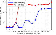
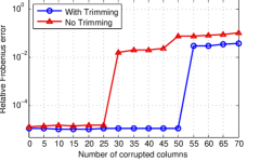
(a)	(b)

Figure 1: Comparison of the performance of Algorithm 1 with and without trimming. The plots show the relative Frobenius norm errors on recovering the uncorrupted columns of a $400\times 400$ rank-$2$ matrix with observation probabilities (a) $p=0.2$, (b) $p=0.3$. Each point in the plots is the average of $10$ trials.

4.2.2 Comparison with standard matrix completion and $L+S$

While our theory and algorithm allow for the corrupted columns of $C_{0}$ to have entries with arbitrarily large magnitude, we perform comparison in a more realistic setting with bounded corruption. In the second set of experiments, the $n_{c}$ non-zero columns of $C_{0}$ are identical, which equal the first column of $L_{0}$ on the locations of its observed entries, and are i.i.d. standard Gaussian on the other locations. These columns are normalized to have the same norm as the first column of $L_{0}$. The locations of the observed entries are also identical across the columns of $C_{0}$, and are randomly selected according to the Bernoulli model with probability $p$. Note that the columns of $C_{0}$ have the same norm and observation probabilities as the authentic columns. If we think of each column of $L_{0}$ as the ratings of movies from an authentic user, then the above construction of $C_{0}$ mimics a rating manipulation scheme that is reported to be effective in the literature [47]. In particular, the columns of $C_{0}$ are meant to be similar to the ratings from an authentic user in $L_{0}$ on the observed locations, while trying to skew the unobserved ones in a coordinated fashion.

When only a small fraction of the entries are observed, the corrupted columns $\mathcal{P}_{\Omega}(C_{0})$ can be viewed as a sparse matrix. Therefore, to separate $L_{0}$ from $\mathcal{P}_{\Omega}(C_{0})$, one might think it is possible to apply the techniques in [9, 14], dubbed the $L+S$ approach, which decomposes a low-rank matrix and a sparse matrix from their sum. In particular, one tries to decompose the input matrix $\mathcal{P}_{\Omega}(M)$ by solving the following convex program:

$$\left(L^{*},S^{*}\right)=\arg \min_{L,S}\;\left\|L\right\|_{*}+\lambda\left\|S\right\|_{1}$$ (7)

$$\text{s.t. }\mathcal{P}_{\Omega}(L+S)=\mathcal{P}_{\Omega}(M).$$

However, a central assumption of the $L+S$ approach, namely, the support of the sparse matrix is spread out over the columns and rows, is violated in the setup considered in this paper. Therefore, it is no surprise that using the $L+S$ approach should not be successful. This is indeed the case, as is illustrated numerically in our experiments.

In particular, we compare our algorithm with the $L+S$ approach (with $\lambda$ set to $1/\sqrt{\max\left(m,n\right)}$ according to [9]), as well as with standard matrix completion (which is equivalent to solving (7) with the additional constraint $S=0$). The convex program (7) is solved using the ADMM methods in [34]. The results are shown in Figure 2 for various values of $p$ and $n_{c}$. We see that the $L+S$ and standard matrix completion approaches are not robust under our setting, and our algorithm has consistently better performance under both metrics considered. Moreover, with a higher observation probability $p$, we can handle a larger number $n_{c}$ of corrupted columns and achieve essentially exact recovery, which is consistent with our theory.

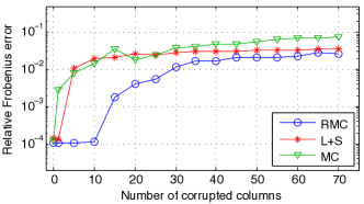
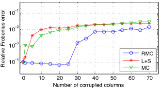
(a)	(b)

Figure 2: Comparison of robust matrix completion in Algorithm 1 (RMC), standard matrix completion (MC) and the $L+S$ approach. The relative Frobenius norm errors are shown for recovering a $400\times 400$ rank-$4$ matrix with observation probabilities (a) $p=0.2$ and (b) $p=0.4$. Each point in the plots is the average of $10$ trials.

4.2.3 Random Corruption

In this third set of experiments, we consider a more benign setting of the corrupted columns, where these columns are generated randomly and independently with i.i.d. Gaussian entries. The experiments are done under the setting with rank $r=4$, $m=200$ rows and $n+n_{c}=1000$ columns. Figure 3 shows the performance of the three algorithms for various $p$ and $n_{c}$. Our algorithm again outperforms standard matrix completion and the $L+S$ approaches. Perhaps more importantly, we see that our algorithm succeeds under a much higher value of $n_{c}$ than in the adversarial setting above. In particular, we recover the authentic columns even when they are significantly out-numbered by the corrupted columns, e.g., with $n=200$ and $n_{c}=800$. This result shows that with such “less adversarial” corruption, the performance of our algorithm is better than is guaranteed by our theory on worse case corruption. Rigorously characterizing this phenomenon is an interesting future direction.

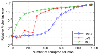
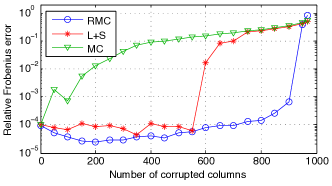
(a)	(b)

Figure 3: Comparison of robust matrix completion in Algorithm 1 (RMC), standard matrix completion (MC) and the $L+S$ approach, with randomly corrupted columns. The relative Frobenius norm errors are shown for recovering a $200\times 1000$ rank-$4$ matrix with observation probabilities (a) $p=0.3$ and (b) $p=0.6$. Each point in the plots is the average of $10$ trials.

Finally, we demonstrate the applicability of our algorithms to larger matrices with sparse observation. We consider a setting with rank $r=8$, $m=1000$ rows and $n+n_{c}=5000$ columns, with observation probability $p=0.05$ or $p=0.1$. The performance of our algorithm is shown in Figure 4. Again we see that our algorithm is able to recover the true matrix even when there are many corrupted columns. The average running time of each trial is less than 2 minutes, indicating scalability to large problems.

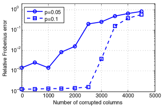
Figure 4: Performance of our Algorithm 1 with random corruption. The relative Frobenius norm errors are shown for recovering a $1000\times 5000$ rank-$8$ matrix with randomly corrupted columns and observation probabilities (a) $p=0.05$ and (b) $p=0.1$. Each point is the average of $10$ trials.

5 Proof of Theorem 1

In this section we prove the main Theorem 1. The proof requires a number of intermediate steps. Here we provide a brief overview of the proof roadmap. By definition of the success of Algorithm 1, we need to show that any optimal solution $\left(L^{*},C^{*}\right)$ of the program (2) has the properties (i) $\mathcal{P}_{I_{0}^{c}}L^{*}=L_{0}$, (ii) $\mathcal{P}_{U_{0}}L^{*}=L^{*}$ and (iii) $I^{*}=\text{column-support}(C^{*})\subseteq I_{0}$. A central roadblock to this goal is that unless the adversary’s corrupted columns happen to be perfectly perpendicular to the column space of the true low-rank matrix, $\left(L^{*},C^{*}\right)$ will not be precisely equal to the ground truth $\left(L_{0},C_{0}\right)$. The reason is simple: if the corrupted columns have a non-perpendicular component, then some part of that will be put into the $L^{*}$ matrix recovered by the optimization. Algorithmically, this matter is irrelevant: as long as the corrupted columns are identified, and the recovered $L^{*}$ matches the desired $L_{0}$ on the non-corrupted columns, our objective is met, and the problem is solved. The analysis, however, is significantly complicated: because $L^{*}\neq L_{0}$ in general and we do not know what $L^{*}$ is exactly, we can no longer use the standard approach in the matrix completion literature of proving the ground-truth is the unique optimal solution of the convex program.

To prove the theorem, we use the idea of a primal-dual witness: we construct a primal solution $(\bar{L},\bar{C})$ and a dual certificate $\bar{Q}$ such that:

• $(\bar{L},\bar{C})$ has the desired properties (i)–(iii);

• $\bar{Q}$ certifies that any optimal solution to (2) is either equal to $\left(\bar{L},\bar{C}\right)$, or is in a subspace defined by $\left(\bar{L},\bar{C}\right)$ and still has the properties (i)–(iii).

Beyond the above obstacle, challenges arise because of the simultaneous presence of three matrix structures: low rank, entry-wise sparse, and column sparse. This requires a number of additional innovations, including concentration bounds involving these structures.

In the rest of the section we present the details of the proof, which is divided into several steps. In Section 5.1, we provide the notation and preliminaries of the proof, and show that it suffices to consider a simpler setting. In Section 5.2 we construct the primal solution $(\bar{L},\bar{C})$ and study its properties. In Section 5.3, we describe the conditions that a dual certificate $\bar{Q}$ needs to satisfy. We construct the dual certificate $\bar{Q}$ in Section 5.4, and then prove that it indeed satisfies the desired conditions with high probability in Section 5.5. The proofs of the technical lemmas are deferred to the appendix.

5.1 Notation and Preliminaries

For a vector $x$, $x_{i}$ is its $i$-th entry. For a matrix $A$, $A_{\cdot j}$ is its $j$-th column and $A_{ij}$ is its $(i,j)$-th entry. Several standard matrix norms are used: $\left\|A\right\|_{\ast}$ is the nuclear norm (the sum of singular values), $\left\|A\right\|$ is the spectral/operator norm (the largest singular values), $\left\|A\right\|_{\infty}$ is the matrix infinity norm (the largest absolute value of the entries), $\left\|A\right\|_{1,2}$ is the sum of $\ell_{2}$ norms of the columns of $A$, $\left\|A\right\|_{\infty,2}$ is the largest $\ell_{2}$ norm of the columns of $A$, and finally $\left\|A\right\|_{F}$ is the Frobenius norm. We also define $\ell_{(\infty,2)^{2}}$ norm of a matrix by $\left\|A\right\|_{(\infty,2)^{2}}:=\max\left\{\left\|A\right\|_{\infty,2},\left\|A^{\top}\right\|_{\infty,2}\right\}$, which is the largest $\ell_{2}$ norm of the columns and rows of $A$. For any positive integer $k$, $[k]:=\left\{1,2,\ldots,k\right\}$. We also use the notation $a\wedge b:=\min\left\{a,b\right\}$ and $a\vee b:=\max\left\{a,b\right\}.$ The letter $c$ and their derivatives ($c_{2}$ etc.) denote unspecified constants that are, however, universal in that they are independent of $p$, $\gamma$, $\beta$, $\rho$, $n$, $n_{c}$, $m$ and $r$. By with high probability (w.h.p.), we mean with probability at least $1-c(m+n)^{-10}$ for some numerical constant $c>0$.

Recall that $\tilde{\Omega}:=\Omega\cap\left([m]\times I_{0}^{c}\right)$ is the set of observed entries on the non-corrupted columns in $I_{0}^{c}$. We use $\Omega_{c}:=\Omega\cap\left([m]\times I_{0}\right)$ to denote the set of observed entries on the corrupted columns in $I_{0}$. We abuse notation by using $\Omega$ (and similarly $\Omega^{c}$, $\tilde{\Omega}$, $\tilde{\Omega}^{c}$ etc) to denote both the set of matrix entries and the linear subspace of matrices supported on these entries. Similarly $I_{0}$ and $I_{0}^{c}$ denote both the set of column indices and the linear subspace of matrices supported on these columns. The operators $\mathcal{P}_{\tilde{\Omega}},\mathcal{P}_{\Omega_{c}},\mathcal{P}_{I_{0}}$ and $\mathcal{P}_{I_{0}^{c}}$ etc. are the corresponding projections onto the sets of matrices supported on $\tilde{\Omega},\Omega_{c},I_{0},I_{0}^{c}$ etc.

Denote the SVD of $L_{0}$ as $U_{0}\Sigma_{0}V_{0}^{\top}$, where $U_{0}\in\mathbb{R}^{m\times r}$ and $V_{0}\in\mathbb{R}^{(n+n_{c})\times r}$. Let $\mathcal{P}_{U_{0}}$ be the projection given by $\mathcal{P}_{U_{0}}A=U_{0}U_{0}^{\top}A$, i.e., projecting each column of $A$ onto the column space of $L_{0}$, where $A$ is any matrix with $m$ rows. The complimentary operation $\mathcal{P}_{U_{0}^{\bot}}A:=A-\mathcal{P}_{U_{0}}A$ projects the columns of $A$ onto the subspace orthogonal to the column space of $L_{0}$. Similarly for the row space we define the projection $\mathcal{P}_{V_{0}}A:=AV_{0}V_{0}^{\top}$. We define the subspace

$$T_{0}:=\{U_{0}X^{\top}+YV_{0}^{\top}:X\in\mathbb{R}^{(n+n_{c})\times r}\text{ with }\mathcal{\mathcal{P}}_{I_{0}}X^{\top}=0,\;Y\in\mathbb{R}^{m\times r}\}\subset\mathbb{R}^{m\times(n+n_{c})},$$

i.e., the set of matrices which has the same column or row space as $L_{0}$ and is supported on the columns in $I_{0}^{c}$; note that $T_{0}\subset I_{0}^{c}.$ The projection $\mathcal{P}_{T_{0}}$ is given by

$$\mathcal{P}_{T_{0}}A:=\mathcal{P}_{U_{0}}A+\mathcal{P}_{V_{0}}A-\mathcal{P}_{U_{0}}\mathcal{P}_{V_{0}}A=\mathcal{P}_{U_{0}}A+\mathcal{P}_{U_{0}^{\bot}}\mathcal{P}_{V_{0}}A$$

for $A\in\mathbb{R}^{m\times(n+n_{c})}$, and the complementary projection is

$$\mathcal{P}_{T_{0}^{\perp}}A:=A-\mathcal{P}_{T_{0}}A=(Id-U_{0}U_{0}^{\top})A(Id-V_{0}V_{0}^{\top}),$$

where $Id$ is the identity matrix with appropriate dimension. We note that the range of $\mathcal{P}_{T_{0}}$ is larger than $T_{0}$ since the matrix $\mathcal{P}_{T_{0}}A$ may have non-zero columns in $I_{0}$. Nevertheless, when restricted to the subspace $I_{0}^{c}$, $\mathcal{P}_{T_{0}}$ is indeed the Euclidean projection onto $T_{0}$. Also note that the column-wise projection $\mathcal{P}_{U_{0}}$ commutes with the row-wise projections $\mathcal{P}_{V_{0}}$, $\mathcal{\mathcal{P}}_{I_{0}}$ and $\mathcal{\mathcal{P}}_{I_{0}^{c}}$, since row-wise projections are given by right multiplying a matrix, whereas column-wise projections are left multiplications. We use $\mathcal{I}$ to denote the identity mapping on $\mathbb{R}^{m\times(n+n_{c})}$.

We provide a summary of the notation used in the proof in Table 1.

Table 1: Summary of Notation

Notation	Meaning
$M$	Input data matrix
$\Omega$	Set of observed indices
$\tilde{\Omega}$	Set of observed indices on the non-corrupted columns
$\Omega_{c}$	Set of observed indices on the corrupted columns
$\hat{\Omega}$	Trimmed set of observed indices
$L^{*},C^{*}$	An optimal solution to the program (2)
$L_{0},C_{0}$	True low-rank matrix and outlier matrix
$U_{0},V_{0},T_{0}$	The left and right singular vectors of $L_{0}$ and the corresponding tangent space
$I_{0}$	Set of the indices of the corrupted columns (i.e., non-zero columns of $C_{0}$)
$\bar{L},\bar{C}$	A solution to the oracle problem (11)
$\bar{U},\bar{V},\bar{T}$	The left and right singular vectors of $\bar{L}$ and the corresponding tangent space
$\bar{I}$	The set of the indices of the non-zero columns of $\bar{C}$
$\bar{H}$	The column-wise normalized version of $\bar{C}$
$\bar{Q}$	The dual certificate corresponding to $\left(\bar{L},\bar{C}\right)$
$\mathcal{P}_{T_{0}},\mathcal{P}_{\bar{U}},\mathcal{P}_{\bar{I}^{c}},\mathcal{P}_{\tilde{\Omega}},$ etc.	Projection operators on $\mathbb{R}^{m\times(n+n_{c})}$
$\mathcal{I}$	The identity mapping on $\mathbb{R}^{m\times(n+n_{c})}$
$Id$	The identity matrix

5.1.1 Equivalent Models and Trimming

It turns out that we may simplify the proof by transferring to an equivalent setting with a simpler observation model and no trimming. Let $\hat{p}:=\min\left\{p,\rho\right\}$ and $\beta:=\frac{\rho}{\hat{p}}$. The conditions for $p,\gamma$ and $\lambda$ in Theorem 1 can be written equivalently as (with possibly different constants $c_{1}$ and $c_{2}$)

$$\hat{p} \geq c_{1}\frac{\mu r\log^{2}(m+n)}{\min(m,n)},$$ (8)

$$\gamma \leq c_{2}\frac{\hat{p}}{\mu r\sqrt{\beta\mu r}\log^{3}(m+n)},$$ (9)

$$\lambda \in\left[\sqrt{\frac{\mu r\log(m+n)}{\hat{p}n}},\frac{1}{48\sqrt{\sqrt{\beta\mu r}\gamma n\log(m+n)}}\right].$$ (10)

We first note that the only randomness in the problem is the distribution of $\tilde{\Omega},$ the set of observed indices on the non-corrupted columns in $I_{0}^{c}$. We claim that it suffices to establish the theorem assuming uniform observation probability on $I_{0}^{c}$. To establish this claim, we need some notation. Without loss of generality we assume $I_{0}^{c}=[n]$. Let $\vec{p}$ be the vector in $\mathbb{R}^{n}_{+}$ with elements $p_{1},\ldots,p_{n}$, where we recall that $p_{j}\geq p\geq\hat{p}$ for all $j\in[n]$ by Assumption 2. Denote by $\mathbb{P}_{\text{Ber}(\vec{p})}$ and $\mathbb{P}_{\text{UBer}(\hat{p}/4)}$ the probabilities calculated respectively when $\tilde{\Omega}$ follows the Bernoulli model with probabilities $\vec{p}=(p_{j})$, and when $\tilde{\Omega}$ follows the Bernoulli model with uniform probability $\hat{p}/4$. The following lemma, proved in the appendix, connects the success probabilities of Algorithm 1 under these two models.

Lemma 1.

Recall that $p_{j}\geq\hat{p}$ for all $j$, and suppose that the condition (8) holds with a sufficiently large constant $c_{1}$. If $\mathbb{P}_{\textrm{UBer}(\hat{p}/4)}\left[success\right]\geq 1-17(m+n)^{-5}$ , then $\mathbb{P}_{\text{Ber}(\vec{p})}\left[success\right]\geq 1-20(m+n)^{-5}$.

The lemma implies that it suffices to prove Theorem 1 assuming $\tilde{\Omega}$ follows the Bernoulli model with uniform probability $\hat{p}/4$.

Now define the set $\Omega^{\prime}:=\tilde{\Omega}\cup\left(\hat{\Omega}\cap([m]\times I_{0})\right)$, which is the set of observed indices with only the columns in $I_{0}$ trimmed. If the condition (8) holds with a sufficiently large constant $c_{1}$, then w.h.p. with respect to $\mathbb{P}_{\textrm{UBer}(\hat{p}/4)}$, $\Omega^{\prime}$ is equal to $\hat{\Omega}$, the fully trimmed set. (This is because by Bernstein’s inequality, each uncorrupted column in $I_{0}^{c}$ has no more than $2\cdot\frac{\hat{p}}{4}m\leq\rho m$ observed entries w.h.p. and therefore is not changed by trimming.) In other words, the convex program (2) with $\Omega^{\prime}$ as the input is identical to the one with input $\hat{\Omega}$ w.h.p., so it suffices to prove Algorithm 1 succeeds w.h.p. assuming the columns in $I_{0}^{c}$ are not trimmed. Finally, note that after trimming the number of remaining observations on each corrupted column in $I_{0}$ is at most $\rho m$. Combining these observations, we conclude that we may replace the sampling Assumption 2 with the following new Assumption 3, and study Algorithm 1 without trimming (i.e., only the convex program). Note that in Assumption 3 we have changed the probability from $\hat{p}/4$ to $\hat{p},$ which only affects the constant $c_{1}$ in the condition (8).

Assumption 3 (Sampling 2).

The set $\tilde{\Omega}$ is sampled from the Bernoulli model with uniform probability $\hat{p}$ on $[m]\times I_{0}^{c}$, and is independent of the locations of the observed entries on the corrupted columns. For each $j\in I_{0}$, we have $\left|\Omega\cap\left([m]\times\{j\}\right)\right|\leq 2\rho m$.

Summarizing the arguments above, we have established that in order to prove Theorem 1, it suffices to prove the following:

Under Assumptions 1 and 3, if the conditions (8)–(10) hold, then with probability at least $1-16(m+n)^{-5}$, the program (2) with $\Omega$ as the input succeeds, i.e., any optimal solution to the program satisfies the properties (i)–(iii) stated at the beginning of this section.

5.2 Primal Construction

We now construct the primal solution $\left(\bar{L},\bar{C}\right)$. Recall that $\Omega_{c}$ is the observed indices on the corrupted columns $I_{0}$. Let $(\bar{L},\bar{C})$ be an optimal solution to the following oracle problem:

$$\min_{L,C} \left\|L\right\|_{*}+\lambda\left\|C\right\|_{1,2}$$ (11)

s.t. $$\mathcal{P}_{\Omega_{c}}(L+C)=\mathcal{P}_{\Omega_{c}}(M)$$

$$\mathcal{\mathcal{P}}_{I_{0}^{c}}(L)=L_{0}.$$

$$\mathcal{P}_{U_{0}}(L)=L$$

$$\mathcal{P}_{I_{0}}(C)=C.$$

Note that we have imposed the desired properties of $\left(L^{*},C^{*}\right)$ as constraints in the oracle problem. Let $\bar{U}\bar{\Sigma}\bar{V}$ be the rank-$r$ SVD of $\bar{L}$ (the lemma below shows that $\bar{L}$ has rank $r$) and $\bar{I}:=\text{column-support}(\bar{C})$. We define several subspaces and projections analogously to those for $L_{0}$: $\mathcal{P}_{\bar{U}}A:=\bar{U}\bar{U}^{\top}A$, $\mathcal{P}_{\bar{U}^{\bot}}A=A-\mathcal{P}_{\bar{U}}A$, $\mathcal{P}_{\bar{V}}:=A\bar{V}\bar{V}^{\top}$, $\bar{T}:=\left\{\bar{U}X^{\top}+Y\bar{V}^{\top}:X\in\mathbb{R}^{(n+n_{c})\times r},Y\in\mathbb{R}^{m\times r}\right\}$, $\mathcal{P}_{\bar{T}}A:=\mathcal{P}_{\bar{U}}A+\mathcal{P}_{\bar{V}}A-\mathcal{P}_{\bar{U}}\mathcal{P}_{\bar{V}}A$, and $\mathcal{P}_{\bar{T}^{\bot}}A:=A-\mathcal{P}_{\bar{T}}A$.

The following lemma, whose proof is given in the appendix, relates some basic properties of the oracle solution $(\bar{L},\bar{C})$ to the ground truth $(L_{0},C_{0})$.

Lemma 2.

We have the following: (a) $\mathcal{P}_{\bar{U}}=\mathcal{P}_{U_{0}}$ and $\bar{I}\subseteq I_{0}$; (b) $\max_{1\leq j\leq n+n_{c}}\left\|\left(\mathcal{\mathcal{P}}_{I_{0}^{c}}\bar{V}^{\top}\right)e_{j}\right\|_{2}\leq\sqrt{\frac{\mu r}{n}}$; (c) $\mathcal{\mathcal{P}}_{I_{0}^{c}}\mathcal{\mathcal{P}}_{\bar{T}}=\mathcal{\mathcal{P}}_{T_{0}}\mathcal{\mathcal{P}}_{I_{0}^{c}}\mathcal{\mathcal{P}}_{\bar{T}}$; (d) $\mathcal{\mathcal{P}}_{\bar{T}}\mathcal{\mathcal{P}}_{I_{0}^{c}}=\mathcal{\mathcal{P}}_{\bar{T}}\mathcal{\mathcal{P}}_{T_{0}}\mathcal{\mathcal{P}}_{I_{0}^{c}}$; (e) $\mathcal{P}_{\bar{T}^{\bot}}\mathcal{P}_{T_{0}^{\bot}}\mathcal{\mathcal{P}}_{I_{0}^{c}}=\mathcal{P}_{T_{0}^{\bot}}\mathcal{\mathcal{P}}_{I_{0}^{c}}$.

Since all the constraint in (11) are linear, by standard convex analysis the optimal solution $(\bar{L},\bar{C})$ must satisfy the KKT conditions. That is, there exist Lagrange multipliers $A_{1}$, $A_{2}$, $A_{3}$ and $A_{4}$ (corresponding to the four constraints in the oracle problem) and matrices $F$ and $G$ such that $\mathcal{P}_{\bar{T}}F=0$ , $\left\|F\right\|\leq 1$, $\mathcal{P}_{\bar{I}^{c}}\bar{H}=0$, $\bar{H}_{\cdot j}=\bar{C}_{\cdot j}/\left\|\bar{C}_{\cdot j}\right\|_{2}$ for all $j\in\bar{I}$, $G\in\bar{I}^{c}$, $\left\|G\right\|_{\infty,2}\leq 1$, and

$$\bar{U}\bar{V}^{\top}+F+\mathcal{\mathcal{P}}_{I_{0}^{c}}A_{2}+\left(\mathcal{I}-\mathcal{P}_{U_{0}}\right)A_{3}=\lambda\left(\bar{H}+G\right)+\mathcal{P}_{I_{0}^{c}}A_{4}=\mathcal{P}_{\Omega_{c}}A_{1};$$ (12)

here $\bar{U}\bar{V}^{\top}+F$ is a subgradient of $\left\|L\right\|_{*}$ at $\bar{L}$, and $\bar{H}+G$ is a subgradient of $\left\|C\right\|_{1,2}$ at $\bar{C}$. Also note that $\bar{H}$ is the column-wise normalized version of $\bar{C}$ with unit-norm nonzero columns. Define the matrix $\bar{H}^{\prime}:=\bar{H}+\mathcal{\mathcal{P}}_{I_{0}}G$. The following lemma characterizes $\bar{H}^{\prime}$ and is proved in the appendix

Lemma 3.

We have the following: (a) $\bar{H}^{\prime}\in\Omega_{c}$; (b) $\mathcal{P}_{\bar{I}}\bar{H}^{\prime}=\bar{H}$; (c) $\left\|\mathcal{\mathcal{P}}_{\bar{I}^{c}}\bar{H}^{\prime}\right\|_{\infty 2}\leq 1$; (d) $\bar{U}\mathcal{P}_{I_{0}}\bar{V}^{\top}=\mathcal{P}_{U_{0}}(\lambda\bar{H}^{\prime})$; (e) $\bar{H}$ and $\bar{H}^{\prime}$ are independent of $\tilde{\Omega}$.

5.3 Success Condition

Recall that in Section 5.1.1 we show that it suffices to prove the convex program (2) succeeds without trimming. The following proposition, proved in the appendix, provides a deterministic sufficient condition for such success. The success condition involves the quantities $\bar{T}$, $\bar{U}$, $\bar{V}$, $\bar{I}$ and $\bar{H}$ of the oracle solution $(\bar{L},\bar{C})$ constructed in the last subsection.

Proposition 1.

If the following conditions hold:

1. $\left\|\left(\hat{p}^{-1}\mathcal{\mathcal{P}}_{T_{0}}\mathcal{P}_{\tilde{\Omega}}\mathcal{\mathcal{P}}_{T_{0}}-\mathcal{\mathcal{P}}_{T_{0}}\right)Z\right\|_{F}\leq\frac{1}{2}\left\|Z\right\|_{F}$ for all $Z\in I_{0}^{c}$.

2. $I_{0}\cap\textrm{range}\left(\mathcal{P}_{\bar{V}}\right)=\{0\}$.

3. There exists a matrix $\bar{Q}\in\mathbb{R}^{m\times(n+n_{c})}$ (called an approximate dual certificate) which satisfies

   1. $\bar{Q}\in\Omega$;

   2. $\bar{U}\bar{V}^{\top}-\mathcal{P}_{\bar{T}}\bar{Q}=\mathcal{P}_{\bar{T}}D$ for some $D\in\mathbb{R}^{m\times(n+n_{c})}$ with $D\in I_{0}^{c}$ and $\left\|D\right\|_{F}\leq\sqrt{\frac{\hat{p}}{2}}\min\left\{\frac{1}{4},\frac{\lambda}{4}\right\}$;

   3. $\left\|\mathcal{P}_{\bar{T}^{\bot}}\bar{Q}\right\|\leq\frac{1}{2}$;

   4. $\mathcal{P}_{\bar{I}}\bar{Q}=\lambda\bar{H}$;

   5. $\left\|\mathcal{P}_{\bar{I}^{c}\cap I_{0}}\bar{Q}\right\|_{\infty,2}\leq\lambda$;

   6. $\left\|\mathcal{\mathcal{P}}_{I_{0}^{c}}\bar{Q}\right\|_{\infty,2}\leq\frac{\lambda}{2}$.

Then any optimal solution $(L^{*},C^{*})$ to the program (2) must satisfy $\mathcal{P}_{I_{0}^{c}}L^{*}=L_{0}$, $\mathcal{P}_{U_{0}}L^{*}=L^{*}$ and $\mathcal{P}_{I_{0}}C^{*}=C^{*}$, which means Algorithm 1 succeeds.

5.3.1 Approximate Isometry and Contraction

We now show that the conditions 1 and 2 in Proposition 1 are satisfied w.h.p. under our model assumptions and the conditions (8)–(10). Recall that by Assumption 3 the set $\tilde{\Omega}$ follows the Bernoulli model with uniform probability $\hat{p}$. The following lemma establishes the approximate isometry property in the condition 1.

Lemma 4.

Suppose $\hat{p}\geq\frac{\mu r}{m\wedge n}\log(m+n)$, then w.h.p. we have: for all $Z\in I_{0}^{c}$,

$$\left\|\left(\hat{p}^{-1}\mathcal{\mathcal{P}}_{T_{0}}\mathcal{P}_{\tilde{\Omega}}\mathcal{\mathcal{P}}_{T_{0}}-\mathcal{\mathcal{P}}_{T_{0}}\right)Z\right\|_{F}\leq\frac{1}{2}\left\|Z\right\|_{F}.$$ (13)

The lemma is a variant of the standard approximate isometry inequality in the literature of matrix completion/decomposition [9, 17, 33]. In particular, we note that the operator $\hat{p}^{-1}\mathcal{\mathcal{P}}_{T_{0}}\mathcal{P}_{\tilde{\Omega}}\mathcal{\mathcal{P}}_{T_{0}}-\mathcal{\mathcal{P}}_{T_{0}}$ maps the subspace $T_{0}\subset I_{0}^{c}$ to itself, so Lemma 4 is an immediate consequence of Part 1) of Lemma 11 in [17].

The next lemma, proved in the appendix, shows that the operator $\mathcal{P}_{\bar{V}}\mathcal{\mathcal{P}}_{I_{0}}\mathcal{P}_{\bar{V}}$ is a contraction, which in particular implies the condition 2 in Proposition 1.

Lemma 5.

If $\lambda^{2}\leq\frac{1}{2\gamma n}$ , then $\left\|\mathcal{P}_{\bar{V}}\mathcal{\mathcal{P}}_{I_{0}}\mathcal{P}_{\bar{V}}(Z)\right\|_{F}\leq\frac{1}{2}\left\|Z\right\|_{F}$ and $\left\|\mathcal{P}_{\bar{V}}\mathcal{\mathcal{P}}_{I_{0}}\mathcal{P}_{\bar{V}}(Z)\right\|\leq\frac{1}{2}\left\|Z\right\|$ for any matrix $Z$.

Note that the requirements on $\hat{p}$ and $\lambda$ in the above lemmas are satisfied under the conditions (8) and (10). We therefore have established the conditions 1 and 2 in Proposition 1. To prove the theorem, it remains to construct a dual certificate $\bar{Q}$ obeying the conditions $3(a)$–$(f)$ in Proposition 1 w.h.p., which is done in the next subsection.

5.4 Dual Construction

We build $\bar{Q}$ in two steps. In the first step we construct a matrix $Q$ that satisfies all the requirements except $3(a)$. By Lemma 5, we know the operator $\mathcal{P}_{\bar{V}}\mathcal{P}_{I_{0}^{c}}\mathcal{P}_{\bar{V}}=\mathcal{P}_{\bar{V}}-\mathcal{P}_{\bar{V}}\mathcal{\mathcal{P}}_{I_{0}}\mathcal{P}_{\bar{V}}$ is invertible on $\textrm{range}\left(\mathcal{P}_{\bar{V}}\right)$ (as a subspace of $\mathbb{R}^{m\times(n+n_{c})}$), with its inverse given by

$$\mathcal{B}:=\left(\mathcal{P}_{\bar{V}}\mathcal{P}_{I_{0}^{c}}\mathcal{P}_{\bar{V}}\right)^{-1}=\mathcal{P}_{\bar{V}}+\sum_{i=1}^{\infty}\left(\mathcal{P}_{\bar{V}}\mathcal{\mathcal{P}}_{I_{0}}\mathcal{P}_{\bar{V}}\right)^{i}.$$ (14)

We define a matrix $Q$ by

$$Q:=\bar{U}\bar{V}^{\top}+\lambda\bar{H}^{\prime}-\lambda\mathcal{P}_{U_{0}}\bar{H}^{\prime}-\mathcal{P}_{I_{0}^{c}}\mathcal{P}_{\bar{V}}\mathcal{B}\mathcal{P}_{\bar{V}}\mathcal{P}_{\bar{U}^{\bot}}\left(\lambda\bar{H}^{\prime}\right).$$

It is straightforward to check that $Q$ has the following properties (proof in the appendix):

Lemma 6.

We have $\mathcal{P}_{I_{0}}Q=\lambda\bar{H}^{\prime}$, $\mathcal{P}_{\bar{T}}Q=\bar{U}\bar{V}^{\top}$, and

$$\left\|\mathcal{P}_{\bar{V}}\mathcal{P}_{\bar{U}^{\bot}}(\lambda\bar{H}^{\prime})\right\|\leq\left\|\lambda\bar{H}^{\prime}\right\|\leq\left\|\lambda\bar{H}^{\prime}\right\|_{F} \leq\lambda\sqrt{\gamma n}.$$

While not needed in the sequel, it is a simple exercise to check that Lemmas 6 and 5 together imply $\left\|\mathcal{P}_{\bar{T}^{\bot}}Q\right\|\leq 3\lambda\sqrt{\gamma n}\leq\frac{1}{2}$ and $\left\|\mathcal{\mathcal{P}}_{I_{0}^{c}}Q\right\|_{\infty,2}\leq\left(1+2\lambda\sqrt{\gamma n}\right)\sqrt{\frac{\mu r}{n}}\leq\frac{1}{2}\lambda$ under the condition (10). Therefore, $Q$ satisfies the condition 3 in Proposition 1 except for the requirement of being an element of $\Omega$. Note that this requirement can only potentially fail on the columns in $I_{0}^{c}$ since $\mathcal{P}_{I_{0}}Q=\lambda\bar{H}^{\prime}\in\Omega_{c}$. As the second step of building the dual certificate, we use the a variant of the golfing scheme in [19] to convert $Q$ to a matrix $\bar{Q}$ that obeys this requirement. Set $k_{0}=20\log(m+n)$ and $p^{\prime}=1-(1-\hat{p})^{1/k_{0}}$. Let $\tilde{\Omega}_{k}$, $k=1,\ldots,k_{0}$ be sets of entries sampled independently from the Bernoulli model on $[m]\times I_{0}^{c}$ with uniform probability $p^{\prime}$; that is, $\mathbb{P}\left((i,j)\in\tilde{\Omega}_{k}\right)=p^{\prime}$ independently of all others for all $(i,j)\in[m]\times I_{0}^{c}$ and $k\in[k_{0}]$. We may assume $\tilde{\Omega}=\bigcup_{k=1}^{k_{0}}\tilde{\Omega}_{k}$, which does not change the distribution of $\tilde{\Omega}$. Note that $p^{\prime}\geq\hat{p}/k_{0}\geq c_{1}\frac{\mu r\log(m+n)}{20(m\wedge n)}$ under the condition (8). We set $Y_{0}:=0$ and define the matrices $\left\{Y_{k}\right\}$ recursively by

$$Y_{k}:=Y_{k-1}+\frac{1}{p^{\prime}}\mathcal{P}_{\tilde{\Omega}_{k}}\mathcal{P}_{T_{0}}\left(\mathcal{P}_{I_{0}^{c}}Q-Y_{k-1}\right),k=1,\ldots,k_{0}.$$

The final dual certificate is given by $\bar{Q}=\mathcal{P}_{I_{0}}Q+Y_{k_{0}}.$

5.5 Verification of the Dual Certificate

We now verify that the dual certificate $\bar{Q}$ constructed above satisfies all the requirements $3(a)$–$3(f)$ in Proposition 1 under the conditions (8)–(10). We have $\mathcal{\mathcal{P}}_{I_{0}^{c}}\bar{Q}=Y_{k_{0}}\in\tilde{\Omega}$ by construction and $\mathcal{P}_{I_{0}}\bar{Q}=\mathcal{P}_{I_{0}}Q=\lambda\bar{H}^{\prime}\in\Omega_{c}$ by part $(a)$ of Lemma 3, so the condition $3(a)$ holds. Moreover, by part $(b)$ and $(c)$ of Lemma 3 we have $\mathcal{\mathcal{P}}_{\bar{I}}\bar{Q}=\lambda\mathcal{\mathcal{P}}_{\bar{I}}\bar{H}^{\prime}=\bar{H}$ and $\left\|\mathcal{P}_{\bar{I}^{c}\cap I_{0}}\bar{Q}\right\|_{\infty.2}=\lambda\left\|\mathcal{P}_{\bar{I}^{c}\cap I_{0}}\bar{H}^{\prime}\right\|_{\infty,2}\leq\lambda$, so the conditions $3(d)$ and $3(e)$ are also satisfied. It remains to verify $3(b)$, $3(c)$ and $3(f)$.

5.5.1 Condition $3(b)$

Define the linear operators $\mathcal{A}_{k}:=\mathcal{\mathcal{P}}_{T_{0}}-\frac{1}{p^{\prime}}\mathcal{\mathcal{P}}_{T_{0}}\mathcal{P}_{\tilde{\Omega}_{k}}\mathcal{\mathcal{P}}_{T_{0}}$ for $k=1,\ldots,k_{o}$ and the matrices $D_{k}=\mathcal{\mathcal{P}}_{T_{0}}\left(\mathcal{\mathcal{P}}_{I_{0}^{c}}Q-Y_{k}\right)$ for $k=0,\ldots,k_{0}$. With this notation, we have $Y_{k}=Y_{k-1}+\frac{1}{p^{\prime}}\mathcal{P}_{\tilde{\Omega}_{k}}D_{k-1}$ by definition, which implies

$$D_{k}=\left(\mathcal{\mathcal{P}}_{T_{0}}-\frac{1}{p^{\prime}}\mathcal{\mathcal{P}}_{T_{0}}\mathcal{P}_{\tilde{\Omega}_{k}}\mathcal{\mathcal{P}}_{T_{0}}\right)D_{k-1}=\mathcal{A}_{k}(D_{k-1}),\;k=1,\ldots,k_{0}.$$ (15)

It follows that with high probability,

$$\left\|D_{k_{0}}\right\|_{F}=\left\|\mathcal{A}_{k_{0}}\mathcal{A}_{k_{0}-1}\cdots\mathcal{A}_{1}\left(D_{0}\right)\right\|_{F}\overset{(a)}{\leq}\frac{1}{2^{k_{0}}}\left\|D_{0}\right\|_{F}\overset{(b)}{\leq}\frac{1}{(m+n)^{10}}\left\|D_{0}\right\|_{F},$$

where $(a)$ follows from Lemma 4 with $\tilde{\Omega}$ replaced by $\tilde{\Omega}_{k}$ and $(b)$ follows from our choice of $k_{0}$. To bound $\left\|D_{0}\right\|_{F}$, we observe that by definition of $Q$,

$$D_{0}=\mathcal{P}_{T_{0}}\mathcal{P}_{I_{0}^{c}}Q =\bar{U}\mathcal{\mathcal{P}}_{I_{0}^{c}}\bar{V}^{\top}+\mathcal{P}_{V_{0}}\mathcal{P}_{I_{0}^{c}}\mathcal{P}_{\bar{V}}\mathcal{B}\mathcal{P}_{\bar{V}}\mathcal{P}_{\bar{U}^{\bot}}\left(\lambda\bar{H}^{\prime}\right)$$ (16)

By (14) and Lemma 5, we know that for any matrix $Z$,

$$\left\|\mathcal{B}(Z)\right\|_{F}\leq\sum_{i=0}^{\infty}\left(\frac{1}{2}\right)^{i}\left\|Z\right\|_{F}\leq 2\left\|Z\right\|_{F}.$$ (17)

Combining the last two equations (16) and (17) gives

$$\left\|D_{0}\right\|_{F}\leq\left\|\bar{U}\bar{V}^{\top}\right\|_{F}+2\left\|\lambda\bar{H}^{\prime}\right\|_{F}\leq\sqrt{r}+2\lambda\sqrt{\gamma n},$$

where the last inequality follows from Lemma 6. It follows that

$$\left\|D_{k_{0}}\right\|_{F}\leq\frac{1}{(m+n)^{10}}\left(\sqrt{r}+2\lambda\sqrt{\gamma n}\right)\leq\frac{\sqrt{\hat{p}}}{2}\min\left\{\frac{1}{4},\frac{\lambda}{4}\right\},$$ (18)

where the last inequality follows from the conditions (8) and (10). On the other hand, since $\bar{Q}=\mathcal{\mathcal{P}}_{I_{0}^{c}}Y_{k_{0}}+\mathcal{\mathcal{P}}_{I_{0}}Q$ and $\mathcal{P}_{\bar{T}}Q=\bar{U}\bar{V}^{\top}$ by Lemma , we have

$$\bar{U}\bar{V}-\mathcal{P}_{\bar{T}}\bar{Q} =\mathcal{P}_{\bar{T}}Q-\mathcal{\mathcal{P}}_{\bar{T}}\left(\mathcal{\mathcal{P}}_{I_{0}^{c}}Y_{k_{0}}+\mathcal{\mathcal{P}}_{I_{0}}Q\right)=\mathcal{P}_{\bar{T}}\mathcal{\mathcal{P}}_{I_{0}^{c}}\left(Q-Y_{k_{0}}\right)=\mathcal{\mathcal{P}}_{\bar{T}}D_{k_{0}},$$ (19)

where the last equality follows from Part $(d)$ of Lemma 2. We conclude that the condition 3(b) in Proposition 1 holds by combining (19), (18) and the fact that $D_{k_{0}}\in T_{0}\subseteq I_{0}^{c}$.

5.5.2 Condition $3(c)$

We may write

$$\mathcal{P}_{\bar{T}^{\bot}}\bar{Q} =\mathcal{P}_{\bar{T}^{\bot}}\left(\lambda\bar{H}^{\prime}\right)+\mathcal{P}_{\bar{T}^{\bot}}\mathcal{\mathcal{P}}_{T_{0}}Y_{k_{0}}+\mathcal{P}_{\bar{T}^{\bot}}\mathcal{P}_{T_{0}^{\bot}}Y_{k_{0}}$$

$$=\mathcal{P}_{\bar{T}^{\bot}}\left(\lambda\bar{H}^{\prime}\right)+\left(\mathcal{P}_{\bar{T}^{\bot}}\mathcal{\mathcal{P}}_{T_{0}}\mathcal{\mathcal{P}}_{I_{0}^{c}}Q-\mathcal{P}_{\bar{T}^{\bot}}D_{k_{0}}\right)+\mathcal{P}_{T_{0}^{\bot}}Y_{k_{0}},$$

where the first equality follows from definition of $\bar{Q}$, and the second equality follows from $Y_{k_{0}}\in T_{0}\subseteq I_{0}^{c}$ and part $(e)$ of Lemma 2. Hence we have

$$\left\|\mathcal{P}_{\bar{T}^{\bot}}\bar{Q}\right\|\leq\left\|\lambda\bar{H}^{\prime}\right\|+\left\|D_{k_{0}}\right\|+\left\|\mathcal{P}_{\bar{T}^{\bot}}\mathcal{\mathcal{P}}_{T_{0}}\mathcal{\mathcal{P}}_{I_{0}^{c}}Q\right\|+\left\|\mathcal{P}_{T_{0}^{\bot}}Y_{k_{0}}\right\|.$$

The condition $3(c)$ holds if each of the terms above is upper bounded by $\frac{1}{8}$. By Lemma , we have $\left\|\lambda\bar{H}^{\prime}\right\|\leq\lambda\sqrt{\gamma n}\leq\frac{1}{16}$, where the last inequality holds under the condition (10). In (18) we already showed that $\left\|D_{k_{0}}\right\|\leq\left\|D_{k_{0}}\right\|_{F}\leq\frac{\sqrt{\hat{p}}}{8}\leq\frac{1}{8}$. Moreover, using (16), we have

$$\left\|\mathcal{P}_{\bar{T}^{\bot}}\mathcal{\mathcal{P}}_{T_{0}}\mathcal{\mathcal{P}}_{I_{0}^{c}}Q\right\|\leq\left\|\mathcal{P}_{\bar{V}^{\bot}}\mathcal{P}_{V_{0}}\mathcal{P}_{I_{0}^{c}}\mathcal{P}_{\bar{V}}\mathcal{B}\mathcal{P}_{\bar{V}}\mathcal{P}_{\bar{U}^{\bot}}(\lambda\bar{H}^{\prime})\right\|_{F}\overset{(a)}{\leq}2\left\|\lambda\bar{H}^{\prime}\right\|_{F}\leq\frac{1}{8},$$

where (a) follows (17) and the fact that projections do not increase the Frobenius norm. It remains to bound $\left\|\mathcal{P}_{T_{0}^{\bot}}Y_{k_{0}}\right\|$ by $\frac{1}{8}$.

For brevity we introduce some additional notation. Let $D_{0}^{U}:=\bar{U}\mathcal{\mathcal{P}}_{I_{0}^{c}}\bar{V}$, and $D{}_{0}^{V}:=\mathcal{P}_{\bar{U}^{\bot}}\mathcal{P}_{V_{0}}\mathcal{P}_{I_{0}^{c}}\mathcal{B}\mathcal{P}_{\bar{V}}\left(\lambda\bar{H}^{\prime}\right)$, $D_{k}^{U}:=\mathcal{A}_{k}\mathcal{A}_{k-1}\cdots\mathcal{A}_{1}(D_{0}^{U})$ and $D_{k}^{V}:=\mathcal{A}_{k}\mathcal{A}_{k-1}\cdots\mathcal{A}_{1}(D_{0}^{V})$ for $k=1,\ldots,k_{0}$. Note that for each $k\geq 2$, $D_{k-1}^{U}$ and $D_{k-1}^{V}$ are independent of $\tilde{\Omega}_{k}$ by construction the $\tilde{\Omega}_{k}$’s and part $(e)$ of Lemma 3. With these definitions, we have $D_{k}=D_{k}^{U}+D_{k}^{V}$ for $k=0,\ldots,k_{0}$ by (16) and (15), and hence

$$Y_{k_{0}}=\sum_{k=1}^{k_{0}}\frac{1}{p^{\prime}}\mathcal{P}_{\tilde{\Omega}_{k}}D_{k-1}=\sum_{i=1}^{k_{0}}\frac{1}{p^{\prime}}\mathcal{P}_{\tilde{\Omega}_{k}}D_{k-1}^{U}+\sum_{k=1}^{k_{0}}\frac{1}{p^{\prime}}\mathcal{P}_{\tilde{\Omega}_{k}}D_{k-1}^{V}.$$ (20)

Let $t$ be either $U$ or $V$. Since $D_{k-1}^{t}\in T_{0}$ for each $k$, we have

$$\sum_{k=1}^{k_{0}}\left\|\mathcal{P}_{T_{0}^{\bot}}\frac{1}{p^{\prime}}\mathcal{P}_{\tilde{\Omega}_{k}}D_{k-1}^{t}\right\|=\sum_{k=1}^{k_{0}}\left\|\mathcal{P}_{T_{0}^{\bot}}\left(\frac{1}{p^{\prime}}\mathcal{P}_{\tilde{\Omega}_{k}}D_{k-1}^{t}-D_{k-1}^{t}\right)\right\|\leq\sum_{k=1}^{k_{0}}\left\|\left(\frac{1}{p^{\prime}}\mathcal{P}_{\tilde{\Omega}_{k}}-\mathcal{I}\right)D_{k-1}^{t}\right\|.$$ (21)

To proceed, we need three lemmas involving the norms of a matrix after certain random projections. Recall that $\tilde{\Omega}$ and $\tilde{\Omega}_{k}$ are sampled from the Bernoulli model with uniform probability $\hat{p}$ and $p^{\prime}$, respectively. The first lemma bounds the spectral norm using the $\ell_{\infty}$ and $\ell{}_{(\infty,2)^{2}}$ norm. This lemma is proved in a recent report by the author [15], but we provide a proof in the appendix for completeness.

Lemma 7.

Let $Z$ be a fixed $m\times(n+n_{c})$ matrix in $I_{0}^{c}$. We have w.h.p.

$$\left\|\frac{1}{\hat{p}}\mathcal{P}_{\tilde{\Omega}}Z-Z\right\|\leq\left(\frac{15\log(m+n)}{\hat{p}}\left\|Z\right\|_{\infty}+\sqrt{\frac{60\log(m+n)}{\hat{p}}}\left\|Z\right\|_{(\infty,2)^{2}}\right).$$

The next lemma, standard in matrix completion literature, further controls the $\ell_{\infty}$ norm.

Lemma 8.

[17, Lemma 13, part 1] Let $Z$ be a fixed $m\times(n+n_{c})$ matrix in $T_{0}$. If $\hat{p}>66\frac{\log(m+n)}{m\wedge n}$, then w.h.p. we have

$$\left\|\frac{1}{\hat{p}}\mathcal{\mathcal{P}}_{T_{0}}\mathcal{P}_{\tilde{\Omega}}\mathcal{\mathcal{P}}_{T_{0}}Z-\mathcal{\mathcal{P}}_{T_{0}}Z\right\|_{\infty}\leq\frac{1}{2}\left\|Z\right\|_{\infty}.$$

The third lemma is new, which controls the $\ell_{(\infty,2)^{2}}$ norm. See the appendix for a proof.

Lemma 9.

The following holds for some constant $c_{0}>0$ and any fixed matrix $Z\in T_{0}$. If $\hat{p}\geq c_{0}\frac{\mu r\log(m+n)}{m\wedge n}$, then we have w.h.p.

$$\left\|\frac{1}{\hat{p}}\mathcal{P}_{T_{0}}\mathcal{P}_{\tilde{\Omega}}\mathcal{P}_{T_{0}}Z-\mathcal{P}_{T_{0}}Z\right\|_{\infty,2} \leq\frac{40\log(m+n)}{\hat{p}}\sqrt{\frac{\mu r}{n\wedge m}}\left\|Z\right\|_{\infty}+\sqrt{\frac{250\mu r\log(m+n)}{\hat{p}(n\wedge m)}}\left\|Z\right\|_{\infty,2}$$

$$\leq\frac{1}{2}\sqrt{\frac{\log(m+n)}{\hat{p}}}\left\|Z\right\|_{\infty}+\frac{1}{2}\left\|Z\right\|_{\infty,2}.$$

The same bound holds with the $\left\|\cdot\right\|_{\infty,2}$ norm replaced by the $\left\|\cdot\right\|_{(\infty,2)^{2}}$ norm.

Applying Lemma 7 with $\tilde{\Omega}$ replaced by $\tilde{\Omega}_{k}$ to the R.H.S. of (21) and using $p^{\prime}\geq\frac{\hat{p}}{20\log(m+n)}\gtrsim\frac{\mu r\log(m+n)}{m\wedge n}$ under the condition (8), we have for $t=U$ or $V$,

$$\sum_{k=1}^{k_{0}}\left\|\left(\frac{1}{p^{\prime}}\mathcal{P}_{\tilde{\Omega}_{k}}-\mathcal{I}\right)D_{k-1}^{t}\right\|\leq\sum_{k=1}^{k_{0}}\frac{15\log^{2}(m+n)}{\hat{p}}\left\|D_{k-1}^{t}\right\|_{\infty}+\sum_{k=1}^{k_{0}}\sqrt{\frac{60\log^{2}(m+n)}{\hat{p}}}\left\|D_{k-1}^{t}\right\|_{(\infty,2)^{2}}.$$ (22)

We then apply Lemmas 8 and 9 with $\tilde{\Omega}$ replaced by $\tilde{\Omega}_{k}$ to the two norms in the last R.H.S., which gives

$$\left\|D_{k-1}^{t}\right\|_{\infty} =\left\|\mathcal{A}_{k-1}\mathcal{A}_{i-2}\cdots\mathcal{A}_{1}\left(D_{0}^{t}\right)\right\|_{\infty}\leq\frac{1}{2^{k-1}}\left\|D_{0}^{t}\right\|_{\infty},$$

$$\left\|D_{k-1}^{t}\right\|_{(\infty,2)^{2}} =\left\|\mathcal{A}_{k-1}\mathcal{A}_{i-2}\cdots\mathcal{A}_{1}\left(D_{0}^{t}\right)\right\|_{(\infty,2)^{2}}\leq\frac{1}{2^{k-1}}\left\|D_{0}^{t}\right\|_{(\infty,2)^{2}}+\frac{k-1}{2^{k-1}}\sqrt{\frac{\log^{2}(m+n)}{\hat{p}}}\left\|D_{0}^{t}\right\|_{\infty}.$$

It follows that

$$\sum_{k=1}^{k_{0}}\frac{\log(m+n)}{p^{\prime}}\left\|D_{k-1}^{t}\right\|_{\infty}+\sum_{k=1}^{k_{0}}\sqrt{\frac{\log(m+n)}{p^{\prime}}}\left\|D_{k-1}^{t}\right\|_{(\infty,2)^{2}}\qquad\qquad\qquad$$

$$\leq\frac{6\log^{2}(m+n)}{\hat{p}}\left\|D_{0}^{t}\right\|_{\infty}+2\sqrt{\frac{\log^{2}(m+n)}{\hat{p}}}\left\|D_{0}^{t}\right\|_{(\infty,2)^{2}}.$$ (23)

Combining (20)–(23), we obtain

$$\left\|\mathcal{P}_{T_{0}^{\bot}}Y_{k_{0}}\right\| \leq\frac{90\log^{2}(m+n)}{\hat{p}}\left(\left\|D_{0}^{U}\right\|_{\infty}+\left\|D_{0}^{V}\right\|_{\infty}\right)+16\sqrt{\frac{\log^{2}(m+n)}{\hat{p}}}\left(\left\|D_{0}^{U}\right\|_{(\infty,2)^{2}}+\left\|D_{0}^{V}\right\|_{(\infty,2)^{2}}\right).$$

The following lemma, proved in the appendix, bounds the norms of $D_{0}^{U}$ and $D_{0}^{V}$ above. The lemma relies on the second part of Assumption 3, which is a consequence of the trimming procedure in Algorithm 1.

Lemma 10.

Recall that $\beta:=\frac{\rho}{\hat{p}}$. Under Assumptions 1 and 3, we have

$$\left\|D_{0}^{U}\right\|_{\infty} \leq\sqrt{\frac{\mu^{2}r^{2}}{mn}},$$

$$\left\|D_{0}^{U}\right\|_{\infty,2}\leq\sqrt{\frac{\mu r}{n}}, \quad\left\|D_{0}^{U}\right\|_{(\infty,2)^{2}}\leq\sqrt{\frac{\mu r}{m\wedge n}},$$

$$\left\|D_{0}^{V}\right\|_{\infty}\leq\left\|D_{0}^{V}\right\|_{\infty,2} \leq 4\lambda^{2}\gamma\mu r\sqrt{\beta\hat{p}n},$$

$$\left\|D_{0}^{V}\right\|_{(\infty,2)^{2}}\leq\left\|D_{0}^{V}\right\|_{F} \leq 4\lambda^{2}\gamma n\sqrt{\mu r\beta\hat{p}}.$$

Using this lemma, we conclude that

$$\left\|\mathcal{P}_{T_{0}^{\bot}}Y_{k_{0}}\right\|\leq \frac{90\mu r\log^{2}(m+n)}{\hat{p}\sqrt{mn}}+90\cdot 4\lambda^{2}\gamma\mu r\sqrt{\frac{\beta n}{\hat{p}}}\log^{2}(m+n)+16\sqrt{\frac{\mu r\log^{2}(m+n)}{\hat{p}(m\wedge n)}}$$

$$\quad+48\lambda^{2}\gamma n\sqrt{\mu r\beta}\log(m+n).$$

One checks that each term above is bounded by $\frac{1}{32}$ under the conditions (8) and (10). This means that $\left\|\mathcal{P}_{T_{0}^{\bot}}Y_{k_{0}}\right\|\leq\frac{1}{8}$, proving the condition $3(c)$ in Proposition 1.

5.5.3 Condition $3(f)$

We need to show $\left\|\mathcal{\mathcal{P}}_{I_{0}^{c}}\bar{Q}\right\|_{\infty,2}=\left\|Y_{k_{0}}\right\|_{\infty,2}\leq\frac{\lambda}{2}$. By (20), we have

$$\left\|Y_{k_{0}}\right\|_{\infty,2}$$

$$\leq \underbrace{\sum_{k=1}^{k_{0}}\left\|\left(\frac{1}{p^{\prime}}\mathcal{P}_{\tilde{\Omega}_{k}}-\mathcal{I}\right)D_{k-1}^{U}\right\|_{\infty,2}+\sum_{k=1}^{k_{0}}\left\|D_{k-1}^{U}\right\|_{\infty,2}}_{S_{1}}+\underbrace{\sum_{k=1}^{k_{0}}\left\|\left(\frac{1}{p^{\prime}}\mathcal{P}_{\tilde{\Omega}_{k}}-\mathcal{I}\right)D_{k-1}^{V}\right\|_{\infty,2}+\sum_{k=1}^{k_{0}}\left\|D_{k-1}^{V}\right\|_{\infty,2}}_{S_{2}}.$$ (24)

It suffices to bound each of $S_{1}$ and $S_{2}$ by $\frac{\lambda}{4}$. We need the following lemma, which is proved in the appendix.

Lemma 11.

For any fixed matrix $Z\in T_{0}$, we have w.h.p.,

$$\left\|\frac{1}{\hat{p}}\mathcal{P}_{\tilde{\Omega}}Z-Z\right\|_{\infty,2} \leq\frac{20\log(m+n)}{\hat{p}}\left\|Z\right\|_{\infty}+\sqrt{\frac{50\log(m+n)}{\hat{p}}}\left\|Z\right\|_{\infty,2}.$$

Using the lemma with $\tilde{\Omega}$ replaced by $\tilde{\Omega}_{k}$, we have w.h.p.

$$S_{1} \leq\sum_{k=1}^{k_{0}}\frac{20\log(m+n)}{p^{\prime}}\left\|D_{k-1}^{U}\right\|_{\infty}+2\sum_{k=1}^{k_{0}}\sqrt{\frac{50\log(m+n)}{p^{\prime}}}\left\|D_{k-1}^{U}\right\|_{\infty,2}.$$

Thanks to the second part of Lemma 9, we know that (23) holds with $\left\|\cdot\right\|_{(\infty,2)^{2}}$ replaced by $\left\|\cdot\right\|_{\infty,2}$. Using this, we obtain that w.h.p.

$$S_{1}\leq\frac{120\log^{2}(m+n)}{\hat{p}}\left\|D_{0}^{U}\right\|_{\infty}+4\sqrt{\frac{50\log^{2}(m+n)}{\hat{p}}}\left\|D_{0}^{U}\right\|_{\infty,2}\leq\frac{120\mu r\log^{2}(m+n)}{\hat{p}\sqrt{mn}}+4\sqrt{\frac{50\mu r\log^{2}(m+n)}{\hat{p}n}},$$

where the last inequality follows from Lemma 10. The last R.H.S. is no more than $\frac{\lambda}{4}$ under the conditions (8) and (10).

Turning to the term $S_{2}$ in (24), we apply Lemma 11 with $\tilde{\Omega}$ replaced by $\tilde{\Omega}_{k}$ to obtain that w.h.p.,

$$S_{2} \leq\sum_{k=1}^{k_{0}}\frac{20\log(m+n)}{p^{\prime}}\left\|D_{k-1}^{V}\right\|_{\infty}+2\sum_{k=1}^{k_{0}}\sqrt{\frac{50\log(m+n)}{p^{\prime}}}\left\|D_{k-1}^{V}\right\|_{\infty,2}.$$

Since (23) holds with $\left\|\cdot\right\|_{(\infty,2)^{2}}$ replaced by $\left\|\cdot\right\|_{\infty,2}$, we obtain that w.h.p.,

$$S_{2}\leq\frac{120\log^{2}(m+n)}{\hat{p}}\left\|D_{0}^{V}\right\|_{\infty}+4\sqrt{\frac{50\log^{2}(m+n)}{\hat{p}}}\left\|D_{0}^{V}\right\|_{\infty,2}.$$

It then follows from Lemma 10 that w.h.p.,

$$S_{2}\leq 480\lambda^{2}\gamma\mu r\sqrt{\frac{\beta n}{\hat{p}}}\log^{2}(m+n)+16\lambda^{2}\gamma\mu r\sqrt{50\beta n\log^{2}(m+n)}\leq 600\lambda^{2}\gamma\mu r\sqrt{\frac{\beta n}{\hat{p}}}\log^{2}(m+n).$$

The last R.H.S. is bounded by $\frac{\lambda}{4}$ w.h.p. under the conditions (8) and (10). This establishes the condition 3(f) in Proposition 1. Finally, note that each random event above holds w.h.p., so by the union bound they hold simultaneously with probability at least $1-20(m+n)^{-5}$. This completes the proof of Theorem 1.

6 Proof of Theorem 2

We consider the two conditions (5) and (6) separately.

6.1 Condition (5): $p\leq\frac{\mu r\log(2n)}{2n}$

In this case we use a modified argument from [11, Theorem 1.7] to establish the impossibility of determining the column space (i.e., the left singular vectors). We may assume $n_{c}=0$.

Without loss of generality, assume that $s:=\frac{n}{\mu r}$ is an integer. We use $e_{i}$ to denote the $i$-th standard basis whose dimension will become clear in context. For $k\in[r]$, define the set

$$B_{k}=\left\{(k-1)s+1,(k-1)s+2,\ldots,ks\right\}.$$ (25)

Consider the matrix $L=\sum_{k=1}^{r}u_{k}v_{k}^{\top}\in\mathbb{R}^{n},$ where the (unnormalized) singular vectors $u_{k}\in\mathbb{R}^{n}$ and $v_{k}\in\mathbb{R}^{n}$ are given by

$$u_{k}=\sum_{i\in B_{k}}\omega_{i}e_{i},\quad v_{k}=\sum_{k\in B_{k}}e_{i},$$

where the $\omega_{i}$’s take values in $\left\{-1,1\right\}$. Clearly, $L$ has rank-$r$ and incoherence parameter $\mu$, and is a block diagonal matrix with $r$ blocks of size $s\times s$. In particular, each row of a block is either all $1$ or $-1$ with its sign determined by $\omega_{i}$. An illustration of $L$ is given in Figure 5. Therefore, in order to uniquely determine the left singular vectors $u_{k}$ from the observed entries of $L$, we must be on event that there is at least one observed entry on every row $i$ of each diagonal block, since otherwise there would be no information on $w_{i}$. Under the Bernoulli sampling model in Assumption 2, the probability of this event is $\pi=\left[1-\left(1-p\right)^{s}\right]^{n}.$ Using the premise $2p\leq\frac{\log(2n)}{s}\leq 1$ of the theorem and the inequality $1-x+x^{2}/2>e^{-x},\forall x\geq 0$, we have

$$1-p\geq 1-\frac{\log(2n)}{2s}\geq 1-\frac{\log(2n)}{s}+\frac{\log^{2}(2n)}{2s^{2}}>e^{-\log(2n)/s}.$$

It follows that

$$\pi\leq\exp\left[-n(1-p)^{s}\right]\leq\exp\left[-ne^{-\log 2n}\right]=\exp(-1/2)\leq\frac{3}{4},$$

where the first inequality follows from $1-x\leq e^{-x}$. Therefore, with probability $1-\pi\geq\frac{1}{4}$, there exists one row of a diagonal block that is unobserved, in which case the $u_{k}$’s cannot be determined. It is easy to see that this implies the conclusion of the theorem.

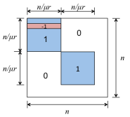
Figure 5: An illustration of $L$ constructed in Section 6.1 with rank $r=2$.

6.2 Condition (6): $\gamma\geq\frac{2p}{\mu r}$

W.L.O.G. we assume $ps$ is a positive integer. Under the above condition, we have $n_{c}=\gamma n\geq 2ps>ps$, where $s:=\frac{n}{\mu r}$ as before. We prove the theorem by constructing a family of candidate solutions $\left(L_{i},C_{i}\right)$, $i=1,2,\ldots,2M$ and showing it is difficult to accurately distinguish them based on the observed data $\Omega$ and $\mathcal{P}_{\Omega}\left(L_{i}+C_{i}\right)$. In this subsection, we use capital letters ($B_{1}$, $I_{2}$, $J$, etc.) to denote sets of column indices (i.e., subsets of $[n+n_{c}]$), and Greek letters ($\Omega,\Theta$, $\xi$ etc.) to denote sets of entry indices (i.e., subsets of $[n]\times[n+n_{c}]$).

Let $J:=\{(r-1)s+1,\ldots,rs+n_{c}\}$. Recall the definition of the $B_{k}$’s in (25), which satisfies $B_{r}\subseteq J$. We further let $I:=J\backslash B_{r}$ and

$$u_{k} =\sum_{i\in B_{k}}e_{i},k\in[r];\quad\bar{u}_{r}=-e_{rs}+\sum_{i\in B_{r},i\neq rs}e_{i};$$

$$v_{k} =\sum_{i\in B_{k}}e_{i},k\in[r];\quad w=\sum_{i\in I}e_{i}.$$

We build two candidate solutions $\left(L_{1},C_{1}\right)$ and $\left(L_{2},C_{2}\right)$ as follows:

$$L_{1}=\sum_{k=1}^{r}u_{k}v_{k}^{\top},\quad C_{1}=\bar{u}_{r}w^{\top}\qquad L_{2}=\sum_{k=1}^{r-1}u_{k}v_{k}^{\top}+\bar{u}_{r}v_{r}^{\top},\quad C_{2}=u_{r}w^{\top}.$$

We illustrate them in Figure 6.

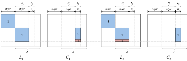
Figure 6: An illustration of $\left(L_{1},C_{1}\right)$ and $\left(L_{2},C_{2}\right)$ constructed in Section 6.2 with rank $r=2$.

Let $M:={s+n_{c}\choose s}$. In the definition of the $\left(L_{1},C_{1}\right)$, if we let the set $B_{k}$ vary in all $M$ possible subsets of $J$ with size $s$ (i.e., we permute the columns in $J$), then we get $M$ different candidates $\left(L_{i},C_{i}\right),i=1,3,\ldots,2M-1$. Similarly, by varying $B_{k}$ in$\left(L_{2},C_{2}\right)$ we can get another $M$ candidates $\left(L_{i},C_{i}\right),i=2,4,\ldots,2M$. We thus have defined a family of $2M$ pairs. Let $I_{i}:=\text{column-support}(C_{i}).$ Note that for the $L_{i}$’s, only the locations of the last $s$ authentic columns vary in $J$, and the sign of these columns’ $rs$-th row changes. The corrupted columns in $C_{i}$ are identical to the last $s$ authentic columns of $L_{i}$ except with the sign of the $rs$-th row flipped. Therefore, to recover the column space of $L_{i}$, one needs to determine the sign of the $rs$-th row. The idea of the proof is simple: under the Bernoulli model and with $n_{c}>2ps$ columns in $I_{i}$, with positive probability the $rs$-row has roughly as many observed $1$’s as $-1$’s, so there is no way to determine which sign is authentic.

We make this precise by specifying the set of observed entries $\Omega=\tilde{\Omega}_{i}\cup\Omega_{c,i}$, for each candidate $i\in[2M]$. According to our assumption, the observations $\tilde{\Omega}_{i}$ on the authentic columns follow the Bernoulli model with uniform probability $p$. It remains to specify the observations $\Omega_{c,i}$ on the corrupted columns. Recall Definition 1 of the Bernoulli model, and let $\Omega_{c,i}^{+}$ be drawn from the Bernoulli model on $[rs-1]\times I_{i}$ with uniform probability $p$; this will be the observed entries on the first $rs-1$ rows of the corrupted columns. Let $\Gamma_{i}$ be independent from $\tilde{\Omega}_{i}$ and drawn according to the Bernoulli model on $[s]$ with uniform probability $p$ . If $\left|\Gamma_{i}\right|\geq n_{c}$, then $\Omega_{c,i}^{-}$, the set of observed entries on the $rs$-th row of the corrupted columns, is set as $\Omega_{c,i}^{-}=\left\{rs\right\}\times I_{i}$. If $\left|\Gamma_{i}\right|=t<n_{c}$, then we set $\Omega_{c_{i}}^{-}=\left\{rs\right\}\times I_{i}\left(t\right)$, where $I_{i}(t)$ denotes the $t$ smallest indices in $I_{i}$. The set of observed entries on the corrupted columns $I_{i}$ is then given by $\Omega_{c,i}=\Omega_{c,i}^{+}\cup\Omega_{c,i}^{-}$. We see that the authentic observations $\tilde{\Omega}_{i}$ are independent of $C_{i}$ and $\Omega_{c,i}$, so Assumption 2 is satisfied. In the sequel, we use $\mathbb{P}_{L_{i},C_{i}}$ to denote the probability computed under the $i$-th candidate solution $\left(L_{i},C_{i}\right)$.

Now suppose the true solution is the first candidate $\left(L_{1},C_{1}\right)$. Let $\Theta_{1}:=\tilde{\Omega}_{1}\cap(\left\{rs\right\}\times J)$ be the set of observations on the $rs$-th row of the authentic columns in $J$. If we define the event

$$\mathcal{E}:=\left\{\left|\Gamma_{1}\right|\leq\left|\Theta_{1}\right|\leq ps\right\},$$

then we have

$$\mathbb{P}_{L_{1},C_{1}}\left[\mathcal{E}\right] \overset{(i)}{\geq}\frac{1}{2}\mathbb{P}_{L_{1},C_{1}}\left[\left|\Gamma_{1}\right|<ps\text{ and }\left|\Theta_{1}\right|<ps\right]$$

$$\overset{(ii)}{\geq}\frac{1}{2}\cdot\mathbb{P}_{L_{1},C_{1}}\left[\left|\Gamma_{1}\right|<ps\right]\cdot\mathbb{P}_{L_{1},C_{1}}\left[\left|\Theta_{1}\right|<ps\right]\overset{(iii)}{\geq}\frac{1}{8}$$

here $(i)$ follows from symmetry, and $(ii)$–$(iii)$ hold because $\left|\Theta_{1}\right|$ and $\left|\Gamma_{1}\right|$ are independent and both follow the Binomial distribution with $s$ trials and probability $p$, whose median is $ps$. On this event $\mathcal{E}$, we can always find another candidate solution $i_{0}\in\left\{2,4,\ldots,2M\right\}$ (which means the last row of $L_{i}$ has a negative sign so the column space is different) such that $\Theta_{1}=\left\{rs\right\}\times I_{i_{0}}\left(\left|\Theta_{1}\right|\right)$; this is because $\Theta_{1}\subseteq\left\{rs\right\}\times J$ and the $I_{i}$’s enumerates the subsets of $J$ with size $n_{c}>ps\geq\left|\Theta_{1}\right|$. See Figure 7 for an illustration. Let $\omega\subseteq[n]\times[n+n_{c}]$ be a realization of $\Omega$ that is consistent with $\mathcal{E}$, i.e., it satisfies $\mathbb{P}_{L_{1},C_{1}}\left[\Omega=\omega\text{ and }\mathcal{E}\right]>0$. We claim that (proved below) for any such $\omega$, we have

$$\mathbb{P}_{L_{1},C_{1}}\left[\Omega=\omega\right] \leq\mathbb{P}_{L_{i_{0}},C_{i_{0}}}\left[\Omega=\omega\right],$$

and

$$\mathcal{P}_{\Omega}\left(L_{1}+C_{1}\right) =Z:=\mathcal{P}_{\Omega}\left(L_{i_{0}}+C_{i_{0}}\right)\quad\quad\text{for }\Omega=\omega.$$

This means the observed data is identical under both candidate solutions, but the $i_{0}$-th candidate has a higher likelihood. In this case, the maximum likelihood estimator (MLE), which is given by

$$f\left(\omega,Z\right):=\arg\max_{(L_{i},C_{i})}\mathbb{P}_{L_{i},C_{i}}\left[\Omega=\omega,\mathcal{P}_{\Omega}\left(L_{i_{0}}+C_{i_{0}}\right)=Z\right]$$

will incorrectly output a solution other than $(L_{1},C_{1})$ with probability at least $\frac{1}{2}$. The above argument in fact holds if any one of the $\left(L_{i},C_{i}\right)$’s is the true solution. Therefore, the average probability of error for the MLE is at least $\frac{1}{2}\cdot\mathbb{P}_{L_{1},C_{1}}\left[\mathcal{E}\right]\geq\frac{1}{16}$. Since the MLE minimizes the average probability of error, which in turn lower bounds the worst case error probability, we conclude that any estimator makes an error with worst case probability at least $\frac{1}{16}$. This proves the theorem.

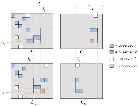
Figure 7: An illustration of the two solutions $\left(L_{1},C_{1}\right)$, $\left(L_{i_{0}},C_{i_{0}}\right)$ and the locations of the observed entries $\Omega$ in Section 6.2, where $\left|\Theta_{1}\right|\leq n_{c}$. In this case the two solutions generate the same observed data $\mathcal{P}_{\Omega}\left(L_{1}+C_{1}\right)=\mathcal{P}_{\Omega}\left(L_{i_{0}}+L_{i_{0}}\right)$ and it is impossible to distinguish between them.

Proof of the claim: When $\Omega=\omega$, the equality $\mathcal{P}_{\Omega}\left(L_{1}+C_{1}\right)=\mathcal{P}_{\Omega}\left(L_{i_{0}}+C_{i_{0}}\right)$ holds by construction of the $\left(L_{i},C_{i}\right)$’s and the assumption on $\omega$ (cf. Figure 7). To prove the inequality, we note the distribution of $\Omega$ under $\left(L_{1},C_{1}\right)$ and $\left(L_{i_{0}},C_{i_{0}}\right)$ only differs on the entries in $\Upsilon:=\left\{rs\right\}\times J$. Let $\xi:=\omega\cap\left(\left\{rs\right\}\times I_{i_{0}}\right)$ and $\zeta:=\omega\cap\left(\left\{rs\right\}\times I_{1}\right).$ Note that because $\omega$ is consistent with $\mathcal{E}$, we have $\left|\zeta\right|\leq\left|\xi\right|\leq ps<n_{c}$; moreover, the observed entries in $\Upsilon$ are either on the columns $I_{i}$ or $I_{i_{0}}$, so $\omega\cap\Upsilon=\xi\cup\zeta$. Let $g(\cdot)$ denote the probability mass function of the Binomial distribution with $s$ trials and probability $p$. Then, according to our specification of $\Omega$ under each candidate solution, we have

$$\frac{\mathbb{P}_{L_{1},C_{1}}\left[\Omega=\omega\right]}{\mathbb{P}_{L_{i_{0}},C_{i_{0}}}\left[\Omega=\omega\right]} =\frac{\mathbb{P}_{L_{1},C_{1}}\left[\Omega\cap\Upsilon=\omega\cap\Upsilon\right]}{\mathbb{P}_{L_{i_{0}},C_{i_{0}}}\left[\Omega\cap\Upsilon=\omega\cap\Upsilon\right]}$$

$$=\frac{p^{\left|\xi\right|}(1-p)^{s-\left|\xi\right|}g(\left|\zeta\right|)}{g(\left|\xi\right|)p^{\left|\zeta\right|}(1-p)^{s-\left|\zeta\right|}}=\frac{g(\left|\zeta\right|)}{g(\left|\xi\right|)}\cdot\left(\frac{p}{1-p}\right)^{\left|\xi\right|-\left|\zeta\right|}.$$

Observe that $g(\cdot)$ is unimodal with mode $ps$, and $\left|\zeta\right|\leq\left|\xi\right|\leq ps$, so $g(\left|\zeta\right|)\leq g(\left|\xi\right|)$. Moreover, we have $\left(\frac{p}{1-p}\right)^{\left|\xi\right|-\left|\zeta\right|}\leq 1$ by the assumption $p\leq\frac{1}{2}$. This means

$$\frac{\mathbb{P}_{L_{1},C_{1}}\left[\Omega=\omega\right]}{\mathbb{P}_{L_{i_{0}},C_{i_{0}}}\left[\Omega=\omega\right]}\leq 1,$$

proving the claim.

7 Conclusion

In this paper, we study the problem of completing a low-rank matrix from sparsely observed entries when observations from some columns are completely and arbitrarily corrupted. We propose a new algorithm based on trimming and convex optimization, and provide performance guarantees showing its robustness to column-wise corruption. We further show that the performance of our algorithm is close to the information-theoretic limit under adversarial corruption, thus achieving near-optimal tradeoffs between sample complexity, robustness and rank.

Immediate future directions include removing the sub-optimality in bounds and allowing for noise and sparse corruption. It may be possible to further improve the robustness of matrix completion by combining our approach with other outlier detection techniques [22, 37]. As our work is motivated by the practical applications in collaborative filtering and crowdsourcing, it is important to study in more depth the computational aspects and develop fast online/parallel algorithms. A more systematic exploration of the relation between sample complexity, model complexity, computational complexity and robustness, will also be of much theoretical and practical interest.

Appendix A Proof of Lemma 1

We need a simple observation first: the convex program (2) has a monotonicity property, that is, having more observed entries on the uncorrupted columns only makes the program more likely to succeed.

Lemma 12 (Monotonicity).

Suppose the indices set $\Omega_{1}$ and $\Omega_{2}$ are such that $\Omega_{1}\cap\left([m]\times I_{0}^{c}\right)\subseteq\Omega_{2}\cap\left([m]\times I_{0}^{c}\right)$ and $\Omega_{1}\cap\left([m]\times I_{0}\right)=\Omega_{2}\cap\left([m]\times I_{0}\right)$. If the program (2) with $\hat{\Omega}=\Omega_{1}$ as the input succeeds, then using $\hat{\Omega}=\Omega_{2}$ as the input also succeeds.

Proof.

Define the set

$$\mathfrak{X}:=\left\{(L,C):\mathcal{P}_{I_{0}^{c}}(L)=L_{0},\mathcal{P}_{U_{0}}(L)=L,\mathcal{P}_{I_{0}}(C)=C,\mathcal{P}_{\Omega_{1}\cap\left([m]\times I_{0}\right)}\left(L+C\right)=\mathcal{P}_{\Omega_{1}\cap\left([m]\times I_{0}\right)}\left(M\right)\right\},$$

which are the solutions that correspond to the success of the algorithm and are consistent on the entries in $\Omega_{1}\cap\left([m]\times I_{0}\right)=\Omega_{2}\cap\left([m]\times I_{0}\right)$. Observe that any solution in $\mathfrak{X}$ is feasible to the program with $\hat{\Omega}$ equal to $\Omega_{1}$ or $\Omega_{2}$. Suppose $(L^{*^{\prime}},C^{*^{\prime}})$ is any optimal solution to the program (2) with $\Omega_{2}$. By optimality we must have $\left\|L^{*^{\prime}}\right\|_{*}+\lambda\left\|C^{*^{\prime}}\right\|_{1,2}\leq\left\|L\right\|_{*}+\lambda\left\|C\right\|_{1,2}$, $\forall\left(L,C\right)\in\mathfrak{X}$. On the other hand, the program with $\Omega_{1}$ succeeds by assumption, meaning that any optimal solution $\left(L^{*},C^{*}\right)$ of it must be in the set $\mathfrak{X}$. It follows that $(L^{*^{\prime}},C^{*^{\prime}})$ has an objective value lower or equal to $(L^{*},C^{*})$. But $(L^{*^{\prime}},C^{*^{\prime}})$ is also feasible to the program with $\Omega_{1}$ since $\Omega_{1}\subseteq\Omega_{2}$, so $(L^{*^{\prime}},C^{*^{\prime}})$ is optimal to the program with $\Omega_{1}$ and hence in the set $\mathfrak{X}$. This means the program with $\Omega_{2}$ succeeds. ∎

We turn to the proof of Lemma 1. Given a vector $\vec{k}\in\mathbb{R}^{n}$ with elements $k_{j}$, let $\mathbb{P}_{\text{Unif}(\vec{k})}$ denote the probability when $\tilde{\Omega}$ follows the uniform model with parameter $\vec{k}$, meaning that the observed entries on the $j$-th column is sampled uniformly at random without replacement from all size-$k_{j}$ subsets of the entries in this column. Recall that $h_{j}$ is the number of observed entries on the $j$-th column before trimming. We use $\left\lfloor x\right\rfloor$ to denote the largest integer no more than $x$. We have the following chain of inequalities:

$$\mathbb{P}_{\text{Ber}(\vec{p})}\left[success\right] =\sum_{k_{1}=1}^{m}\cdots\sum_{k_{n}=1}^{m}\mathbb{P}_{\text{Ber}(\vec{p})}\left[success|h_{j}=k_{j},j\in[n]\right]\mathbb{P}_{\text{Ber}(\vec{p})}\left[h_{j}=k_{j},j\in[n]\right]$$

$$\geq\sum_{k_{1}=\left\lfloor\hat{p}m/2\right\rfloor}^{m}\cdots\sum_{k_{n}=\left\lfloor\hat{p}m/2\right\rfloor}^{m}\mathbb{P}_{\text{Ber}(\vec{p})}\left[success|h_{j}=k_{j},j\in[n]\right]\mathbb{P}_{\text{Ber}(\vec{p})}\left[h_{j}=k_{j},j\in[n]\right]$$

$$\overset{(a)}{=}\sum_{k_{1}=\left\lfloor\hat{p}m/2\right\rfloor}^{m}\cdots\sum_{k_{n}=\left\lfloor\hat{p}m/2\right\rfloor}^{m}\mathbb{P}_{\text{Unif}(\vec{k})}\left[success\right]\mathbb{P}_{\text{Ber}(\vec{p})}\left[h_{j}=k_{j},j\in[n]\right]$$

$$\overset{(b)}{=}\sum_{k_{1}=\left\lfloor\hat{p}m/2\right\rfloor}^{m}\cdots\sum_{k_{n}=\left\lfloor\hat{p}m/2\right\rfloor}^{m}\mathbb{P}_{\text{Unif}\left(\vec{k}\wedge\left\lfloor\rho m\right\rfloor\right)}\left[success\right]\mathbb{P}_{\text{Ber}(\vec{p})}\left[h_{j}=k_{j},j\in[n]\right]$$

$$\overset{(c)}{\geq}\sum_{k_{1}=\left\lfloor\hat{p}m/2\right\rfloor}^{m}\cdots\sum_{k_{n}=\left\lfloor\hat{p}m/2\right\rfloor}^{m}\mathbb{P}_{\text{Unif}\left(\left\lfloor\hat{p}m/2\right\rfloor\right)}\left[success\right]\mathbb{P}_{\text{Ber}(\vec{p})}\left[h_{j}=k_{j},j\in[n]\right]$$

$$=\mathbb{P}_{\text{Unif}\left(\left\lfloor\hat{p}m/2\right\rfloor\right)}\left[success\right]\mathbb{P}_{\text{Ber}(\vec{p})}\left[h_{j}\geq\left\lfloor\hat{p}m/2\right\rfloor,j\in[n]\right]$$

$$\overset{(d)}{\geq}\mathbb{P}_{\text{Unif}\left(\left\lfloor\hat{p}m/2\right\rfloor\right)}\left[success\right]\left(1-(m+n)^{-10}\right),$$

where $(a)$ follows from the fact that the conditional distribution of a set following the Bernoulli model given its cardinality is the same as sampling uniformly without replacement, $(b)$ is a consequence of the trimming step in Algorithm 1, as a uniform subset of a uniformly sampled set is still uniform, $(c)$ follows from $\rho m\geq\hat{p}m/2$ and the monotonicity in Lemma 12, and finally $(d)$ follows from the Bernstein inequality under the condition (8) with $c_{1}$ large enough. The probability in $(d)$ can be bounded by similar reasoning as follows:

$$\mathbb{P}_{\text{Unif}\left(\left\lfloor\hat{p}m/2\right\rfloor\right)}\left[success\right]$$

$$\geq \mathbb{P}_{\text{Unif}\left(\left\lfloor\hat{p}m/2\right\rfloor\right)}\left[success\right]\sum_{k_{1}=1}^{\left\lfloor\hat{p}m/2\right\rfloor}\cdots\sum_{k_{n}=1}^{\left\lfloor\hat{p}m/2\right\rfloor}\mathbb{P}_{\text{UBer}(\hat{p}/4)}\left[h_{j}=k_{j},j\in[n]\right]$$

$$\overset{(a)}{\geq} \sum_{k_{1}=1}^{\left\lfloor\hat{p}m/2\right\rfloor}\cdots\sum_{k_{n}=1}^{\left\lfloor\hat{p}m/2\right\rfloor}\mathbb{P}_{\text{Unif}(\vec{k})}\left[success\right]\mathbb{P}_{\text{UBer}(\hat{p}/4)}\left[h_{j}=k_{j},j\in[n]\right]$$

$$\overset{(b)}{=} \sum_{k_{1}=1}^{\left\lfloor\hat{p}m/2\right\rfloor}\cdots\sum_{k_{n}=1}^{\left\lfloor\hat{p}m/2\right\rfloor}\mathbb{P}_{\text{UBer}(\hat{p}/4)}\left[success|h_{j}=k_{j},j\in[n]\right]\mathbb{P}_{\text{UBer}(\hat{p}/4)}\left[h_{j}=k_{j},j\in[n]\right]$$

$$= \sum_{k_{1}=1}^{\left\lfloor\hat{p}m/2\right\rfloor}\cdots\sum_{k_{n}=1}^{\left\lfloor\hat{p}m/2\right\rfloor}\mathbb{P}_{\text{UBer}(\hat{p}/4)}\left[success,h_{j}=k_{j},j\in[n]\right]$$

$$= \mathbb{P}_{\text{UBer}(\hat{p}/4)}\left[success\right]-\sum_{\vec{k}:\exists j\in[n],k_{j}>\left\lfloor\hat{p}m/2\right\rfloor}\mathbb{P}_{\text{UBer}(\hat{p}/4)}\left[success,h_{j}=k_{j},j\in[n]\right]$$

$$\geq \mathbb{P}_{\text{UBer}(\hat{p}/4)}\left[success\right]-\mathbb{P}_{\text{UBer}(\hat{p}/4)}\left[\exists j\in[n],h_{j}>\left\lfloor p^{\prime}m/2\right\rfloor\right]$$

$$\overset{(c)}{\geq} \mathbb{P}_{\text{UBer}(\hat{p}/4)}\left[success\right]-(m+n)^{-10},$$

where $(a)$ follows from the monotonicity Lemma 12, $(b)$ follows from the fact that conditional Bernoulli distribution is uniform, and $(c)$ follows from the Bernstein inequality under the condition (8). Combining pieces, we obtain

$$\mathbb{P}_{\text{Ber}(\vec{p})}\left[success\right]\geq\left(1-(m+n)^{-10}\right)\left(\mathbb{P}_{\text{UBer}(\hat{p}/4)}\left[success\right]-(m+n)^{-10}\right).$$

The lemma follows.

Appendix B Proof of Lemmas in Section 5.2

In this section, we prove the lemmas used in Section 5.2.

B.1 Proof of Lemma 2

Let $\textrm{col}(Z)$ denote the column space of a matrix $Z$. Observe that $\mathcal{P}_{U_{0}}\bar{L}=\bar{L}$ implies $\textrm{col}(\bar{L})\subseteq\textrm{col}(U_{0})$, and $\mathcal{\mathcal{P}}_{I_{0}^{c}}(\bar{L})=L_{0}$ implies $\textrm{col}(\bar{L})\supseteq\textrm{col}(U_{0})$. It follows that $\textrm{col}(\bar{U})=\textrm{col}(\bar{L})=\textrm{col}(U_{0})$. Because $\bar{C}$ satisfies the last constraint in the oracle problem (11), we have $\bar{I}\in I_{0}$. This proves part (a) of the lemma. A consequence is that $\textrm{rank}(\bar{L})=\textrm{rank}(L_{0})=r$.

Since $\mathcal{\mathcal{P}}_{I_{0}^{c}}\bar{L}=L_{0}$, we conclude that the matrix $\bar{V}_{c}^{\top}:=\mathcal{\mathcal{P}}_{I_{0}^{c}}\bar{V}^{\top}$ has the same rank-$r$ row space as $V_{0}^{\top}$ . Therefore, $\bar{V}_{c}^{\top}\bar{V}_{c}\in\mathbb{R}^{r\times r}$ is positive definite and there exists a symmetric and invertible matrix $K_{1}\in\mathbb{R}^{r\times r}$ with $K_{1}^{2}=\bar{V}_{c}^{\top}\bar{V}_{c}$ and $\left\|K_{1}\right\|\leq\left\|\bar{V}_{c}\right\|\leq\left\|\bar{V}\right\|\leq 1$. This implies that $K_{1}^{-1}\bar{V}_{c}^{\top}$ has orthonormal rows spanning the same row space as $V_{0}^{\top}$. Because $V_{0}^{\top}$ also has orthonormal rows, there must exist an orthonormal matrix $K_{2}\in\mathbb{R}^{r\times r}$ such that $K_{2}K_{1}^{-1}\bar{V}_{c}^{\top}=V_{0}^{\top}$. Hence we have $\bar{V}_{c}^{\top}=NV_{0}^{\top},$ where the matrix $N:=K_{2}^{-1}K_{1}\in\mathbb{R}^{r\times r}$ is invertible. It follows that

$$\max_{1\leq j\leq n+n_{c}}\left\|\left(\mathcal{\mathcal{P}}_{I_{0}^{c}}\bar{V}^{\top}\right)e_{j}\right\|_{2}^{2}=\max_{j}\left\|K_{2}^{-1}K_{1}V_{0}^{\top}e_{j}\right\|_{2}^{2}\leq\left\|K_{2}^{-1}\right\|^{2}\left\|K_{1}\right\|^{2}\max_{j}\left\|V_{0}^{\top}e_{j}\right\|_{2}^{2}\leq\frac{\mu r}{n},$$

where in the last inequality we use the incoherence of $L_{0}$ in Assumption 1. This proves part $(b)$.

Now consider part $(c)$. Let $Z$ be an arbitrary matrix in $\mathbb{R}^{m\times(n+n_{c})}$. By part (a) of the lemma, we have $\mathcal{P}_{U_{0}}\mathcal{P}_{\bar{U}}\left(\mathcal{\mathcal{P}}_{I_{0}^{c}}Z\right)=\mathcal{P}_{\bar{U}}\left(\mathcal{\mathcal{P}}_{I_{0}^{c}}Z\right)$. We also have

$$\mathcal{\mathcal{P}}_{I_{0}^{c}}\mathcal{P}_{\bar{U}^{\bot}}\mathcal{P}_{\bar{V}}Z=\left(\mathcal{P}_{\bar{U}^{\bot}}Z\right)\bar{V}\mathcal{\mathcal{P}}_{I_{0}^{c}}\left(\bar{V}^{\top}\right)=\left(\mathcal{P}_{\bar{U}^{\bot}}Z\right)\bar{V}\bar{V}_{c}^{\top},$$

where the R.H.S. spans the same row space as $V_{0}^{\top}$ by the discussion in the last paragraph. It follows that

$$\mathcal{\mathcal{P}}_{T_{0}}\mathcal{\mathcal{P}}_{I_{0}^{c}}\mathcal{\mathcal{P}}_{\bar{T}}Z =\mathcal{\mathcal{P}}_{T_{0}}\mathcal{P}_{\bar{U}}\mathcal{\mathcal{P}}_{I_{0}^{c}}Z+\mathcal{\mathcal{P}}_{T_{0}}\mathcal{\mathcal{P}}_{I_{0}^{c}}\mathcal{P}_{\bar{U}^{\bot}}\mathcal{P}_{\bar{V}}Z=\mathcal{P}_{\bar{U}}\mathcal{\mathcal{P}}_{I_{0}^{c}}Z+\mathcal{\mathcal{P}}_{I_{0}^{c}}\mathcal{P}_{\bar{U}^{\bot}}\mathcal{P}_{\bar{V}}Z=\mathcal{\mathcal{P}}_{I_{0}^{c}}\mathcal{\mathcal{P}}_{\bar{T}}Z.$$

For part $(d)$, the previous discussion shows that $\bar{V}_{c}=V_{0}N^{\top}$. Therefore, for any $Y\in\mathbb{R}^{m\times(n+n_{c})}$, we have

$$\left(\mathcal{\mathcal{P}}_{I_{0}^{c}}Y\right)V_{0}V_{0}^{\top}\bar{V}\bar{V}^{\top}=\left(\mathcal{\mathcal{P}}_{I_{0}^{c}}Y\right)V_{0}V_{0}^{\top}\bar{V}_{c}\bar{V}^{\top}=\left(\mathcal{\mathcal{P}}_{I_{0}^{c}}Y\right)V_{0}V_{0}^{\top}V_{0}N^{\top}\bar{V}^{\top}=\left(\mathcal{\mathcal{P}}_{I_{0}^{c}}Y\right)\bar{V}_{c}\bar{V}^{\top}=\left(\mathcal{\mathcal{P}}_{I_{0}^{c}}Y\right)\bar{V}\bar{V}^{\top}.$$

Applying this equality with $Y=\mathcal{P}_{\bar{U}^{\bot}}Z$, we obtain

$$\mathcal{\mathcal{P}}_{\bar{T}}\mathcal{\mathcal{P}}_{T_{0}}\mathcal{\mathcal{P}}_{I_{0}^{c}}Z =\mathcal{P}_{\bar{U}}\left(\mathcal{\mathcal{P}}_{I_{0}^{c}}Z\right)+\left(\mathcal{\mathcal{P}}_{I_{0}^{c}}\left(\mathcal{I}-\mathcal{P}_{U_{0}}\right)Z\right)V_{0}V_{0}^{\top}\bar{V}\bar{V}^{\top}=\mathcal{P}_{\bar{U}}\mathcal{\mathcal{P}}_{I_{0}^{c}}Z+\left(\mathcal{\mathcal{P}}_{I_{0}^{c}}\mathcal{P}_{\bar{U}^{\bot}}Z\right)\bar{V}\bar{V}^{\top}=\mathcal{\mathcal{P}}_{\bar{T}}\mathcal{\mathcal{P}}_{I_{0}^{c}}Z.$$

Finally, to prove part $(e)$, we note that

$$\mathcal{P}_{\bar{T}^{\bot}}\mathcal{P}_{T_{0}^{\bot}}\mathcal{\mathcal{P}}_{I_{0}^{c}}Z =\left(\mathcal{I}-\mathcal{\mathcal{P}}_{\bar{T}}\right)\left(\mathcal{I}-\mathcal{\mathcal{P}}_{T_{0}}\right)\mathcal{\mathcal{P}}_{I_{0}^{c}}Z.$$

Expanding the last R.H.S and applying part $(d)$ of the lemma gives the desired result.

B.2 Proof of Lemma 3

Applying $\mathcal{P}_{I_{0}}$ to both sides of the last equality in (12) proves part $(a)$ of the lemma. Part $(b)$ follows from $G\in\bar{I}^{c}$, and part $(c)$ follows from $\mathcal{P}_{\bar{I}^{c}}\bar{H}^{\prime}=\mathcal{P}_{\bar{I}^{c}}\mathcal{P}_{I_{0}}G$. Applying the projection $\mathcal{P}_{\bar{U}}\mathcal{P}_{I_{0}}=\mathcal{P}_{U_{0}}\mathcal{P}_{I_{0}}$ to both sides of the first equality in (12), we obtain part $(d)$. Finally, note that $\bar{H}$ and $\bar{H}^{\prime}$ are determined by the oracle program (11), which only depends on $\mathcal{P}_{\Omega_{c}}M=\mathcal{P}_{\Omega_{c}}C_{0}$ and dose not involve $\tilde{\Omega}$. Therefore, independence between $\tilde{\Omega}$ and $\mathcal{P}_{\Omega_{c}}C_{0}$ imposed in Assumption 3 implies part $(e)$.

Appendix C Proof of Proposition 1

To prove the proposition, we need a technical lemma.

Lemma 13.

Suppose (13) holds, then for any $\Delta_{l},\Delta_{c}\in\mathbb{R}^{m\times(n+n_{c})}$ with $\mathcal{P}_{\Omega}\Delta_{l}+\mathcal{P}_{\Omega}\Delta_{c}=0$, we have

$$\left\|\mathcal{\mathcal{P}}_{I_{0}^{c}}\mathcal{P}_{\bar{T}}\Delta_{l}\right\|_{F}\leq\sqrt{\frac{2}{\hat{p}}}\left(\left\|\mathcal{P}_{\bar{T}^{\bot}}\Delta_{l}\right\|_{*}+\left\|\mathcal{\mathcal{P}}_{I_{0}^{c}}\Delta_{c}\right\|_{1,2}\right).$$

Proof.

Since $\mathcal{P}_{\Omega}\Delta_{c}=-\mathcal{P}_{\Omega}\Delta_{l}$, we have

$$\left\|\mathcal{\mathcal{P}}_{I_{0}^{c}}\Delta_{c}\right\|_{1,2}\geq\left\|\mathcal{P}_{\tilde{\Omega}}\Delta_{c}\right\|_{F} =\left\|\mathcal{P}_{\tilde{\Omega}}\Delta_{l}\right\|_{F}.$$

By triangle inequality, we get

$$\left\|\mathcal{P}_{\tilde{\Omega}}\Delta_{l}\right\|_{F}\geq\left\|\mathcal{P}_{\tilde{\Omega}}\mathcal{P}_{\bar{T}}\Delta_{l}\right\|_{F}-\left\|\mathcal{P}_{\tilde{\Omega}}\mathcal{P}_{\bar{T}^{\bot}}\Delta_{l}\right\|_{F}\geq\left\|\mathcal{P}_{\tilde{\Omega}}\mathcal{P}_{I_{0}^{c}}\mathcal{P}_{\bar{T}}\Delta_{l}\right\|_{F}-\left\|\mathcal{P}_{\bar{T}^{\bot}}\Delta_{l}\right\|_{\ast}.$$

We bound the first term in the last R.H.S.:

$$\left\|\mathcal{P}_{\tilde{\Omega}}\mathcal{P}_{I_{0}^{c}}\mathcal{P}_{\bar{T}}\Delta_{l}\right\|_{F}^{2} =\left\langle\mathcal{P}_{\tilde{\Omega}}\mathcal{P}_{\mathcal{I}_{0}^{c}}\mathcal{P}_{\bar{T}}\Delta_{l},\mathcal{P}_{\tilde{\Omega}}\mathcal{P}_{\mathcal{I}_{0}^{c}}\mathcal{P}_{\bar{T}}\Delta_{l}\right\rangle$$

$$\overset{(a)}{=}\left\langle\mathcal{P}_{\mathcal{I}_{0}^{c}}\mathcal{P}_{\bar{T}}\Delta_{l},\mathcal{\mathcal{P}}_{T_{0}}\mathcal{P}_{\tilde{\Omega}}\mathcal{\mathcal{P}}_{T_{0}}\mathcal{P}_{\mathcal{I}_{0}^{c}}\mathcal{P}_{\bar{T}}\Delta_{l}\right\rangle$$

$$\overset{(b)}{=}\left\langle\mathcal{P}_{\mathcal{I}_{0}^{c}}\mathcal{P}_{\bar{T}}\Delta_{l},\left(\mathcal{\mathcal{P}}_{T_{0}}\mathcal{P}_{\tilde{\Omega}}\mathcal{\mathcal{P}}_{T_{0}}\right)\mathcal{P}_{\mathcal{I}_{0}^{c}}\mathcal{P}_{\bar{T}}\Delta_{l}-\hat{p}\mathcal{P}_{T_{0}}\mathcal{P}_{\mathcal{I}_{0}^{c}}\mathcal{P}_{\bar{T}}\Delta_{l}+\hat{p}\mathcal{P}_{\mathcal{I}_{0}^{c}}\mathcal{P}_{\bar{T}}\Delta_{l}\right\rangle$$

$$\overset{(c)}{\geq}\frac{\hat{p}}{2}\left\|\mathcal{\mathcal{P}}_{I_{0}^{c}}\mathcal{P}_{\bar{T}}\Delta_{l}\right\|_{F}^{2}.$$

where $(a)$ follows from Part (c) of Lemma 2 and the fact that $\mathcal{P}_{T_{0}}$ is a projection when restricted to $I_{0}^{c}$, $(b)$ uses Part (c) of Lemma 2 again, and $(c)$ uses (13). Combining the last three equations proves the lemma. ∎

Back to the proof of Proposition 1. Suppose $\left(L^{*},C^{*}\right)=(\bar{L}+\Delta_{l},\;\bar{C}+\Delta_{c})$ is an optimal solution to (2), with $\mathcal{P}_{\Omega}\Delta_{l}+\mathcal{P}_{\Omega}\Delta_{c}=0$. Take any matrix $F\in\bar{T}^{\perp}$ such that $\left\|F\right\|=1$, $\left\langle F,\;P_{\bar{T}^{\perp}}\Delta_{l}\right\rangle=\left\|P_{\bar{T}^{\perp}}\Delta_{l}\right\|_{\ast}$ and another matrix $G\in\bar{I}^{c}$ such that $\left\|G\right\|_{\infty,2}=1$, $\left\langle G,\;P_{\bar{I}^{c}}\Delta_{c}\right\rangle=\left\|P_{\bar{I}^{c}}\Delta_{c}\right\|_{1,2}=\left\|P_{\bar{I}^{c}\cap I_{0}}\Delta_{c}\right\|_{1,2}+\left\|\mathcal{\mathcal{P}}_{I_{0}^{c}}\Delta_{c}\right\|_{1,2}$. Then $\bar{U}\bar{V}^{\top}+F$ is a subgradient of $\left\|\bar{L}\right\|_{\ast}$ and $P_{\bar{I}}\bar{Q}+\lambda G$ is a subgradient of $\lambda\left\|\bar{C}\right\|_{1,2}$. By optimality of $\left(L^{*},C^{*}\right)$, we have

$$0 \geq\left\|\bar{L}+\Delta_{l}\right\|_{\ast}+\lambda\left\|\bar{C}+\Delta_{c}\right\|_{1,2}-\left\|\bar{L}\right\|_{\ast}-\lambda\left\|\bar{C}\right\|_{1,2}$$

$$\overset{(i)}{\geq}\left\langle\bar{U}\bar{V}^{\top}+F,\Delta_{l}\right\rangle+\left\langle\mathcal{\mathcal{P}}_{I_{0}}\bar{Q}+\lambda G,\Delta_{c}\right\rangle$$

$$\overset{(ii)}{=}\left\|\mathcal{P}_{\bar{T}^{\bot}}\Delta_{l}\right\|_{\ast}+\lambda\left(\left\|\mathcal{P}_{\bar{I}^{c}\cap I_{0}}\Delta_{c}\right\|_{1,2}+\left\|\mathcal{\mathcal{P}}_{I_{0}^{c}}\Delta_{c}\right\|_{1,2}\right)+\left\langle\bar{U}\bar{V}^{\top}-\bar{Q},\Delta_{l}\right\rangle+\left\langle\mathcal{\mathcal{P}}_{\bar{I}}\bar{Q}-\bar{Q},\Delta_{c}\right\rangle$$

where $(i)$ follows from the definition of a subgradient, and $(ii)$ is due to Condition $(a)$ and $\mathcal{P}_{\Omega}\Delta_{l}+\mathcal{P}_{\Omega}\Delta_{c}=0$. Now observe that Conditions $3(b)$ and $3(c)$ imply

$$\left\langle\bar{U}\bar{V}^{\top}-\bar{Q},\;\Delta_{l}\right\rangle=\left\langle\mathcal{\mathcal{P}}_{\bar{T}}D-\mathcal{P}_{\bar{T}^{\bot}}\bar{Q},\;\Delta_{l}\right\rangle\geq-\sqrt{\frac{\hat{p}}{2}}\min\left\{\frac{1}{4},\frac{\lambda}{4}\right\}\left\|\mathcal{\mathcal{P}}_{I_{0}^{c}}\mathcal{\mathcal{P}}_{\bar{T}}\Delta_{l}\right\|_{F}-\frac{1}{2}\left\|\mathcal{P}_{\bar{T}^{\bot}}\Delta_{l}\right\|_{\ast},$$

and Conditions $3(e)$ and $3(f)$ imply

$$\left\langle\mathcal{\mathcal{P}}_{\bar{I}}\bar{Q}-\bar{Q},\Delta_{c}\right\rangle\geq-\lambda\left\|\mathcal{P}_{\bar{I}^{c}\cap I_{0}}\Delta_{c}\right\|_{1,2}-\frac{\lambda}{2}\left\|\mathcal{\mathcal{P}}_{I_{0}^{c}}\Delta_{c}\right\|_{1,2}$$

Putting together, we obtain

$$0 \geq\frac{1}{2}\left\|\mathcal{P}_{\bar{T}^{\bot}}\Delta_{l}\right\|_{\ast}+\frac{1}{2}\lambda\left\|\mathcal{\mathcal{P}}_{I_{0}^{c}}\Delta_{c}\right\|_{1,2}-\sqrt{\frac{\hat{p}}{2}}\left\|\mathcal{\mathcal{P}}_{I_{0}^{c}}\mathcal{\mathcal{P}}_{\bar{T}}\Delta_{l}\right\|_{F}$$

$$\overset{(iii)}{\geq}\frac{1}{2}\left\|\mathcal{P}_{\bar{T}^{\bot}}\Delta_{l}\right\|_{\ast}+\frac{1}{2}\lambda\left\|\mathcal{\mathcal{P}}_{I_{0}^{c}}\Delta_{c}\right\|_{1,2}-\min\left\{\frac{1}{4},\frac{\lambda}{4}\right\}\left(\left\|\mathcal{P}_{\bar{T}^{\bot}}\Delta_{l}\right\|_{*}+\left\|\mathcal{\mathcal{P}}_{I_{0}^{c}}\Delta_{c}\right\|_{1,2}\right)$$

$$\geq\frac{1}{4}\left\|\mathcal{P}_{\bar{T}^{\bot}}\Delta_{l}\right\|_{F}+\frac{1}{4}\lambda\left\|\mathcal{\mathcal{P}}_{I_{0}^{c}}\Delta_{c}\right\|_{1,2}\geq 0,$$

where $(iii)$ follows from Lemma 13. Therefore, we must have

$$\left\|\mathcal{P}_{\bar{T}^{\bot}}\Delta_{l}\right\|_{F}=\left\|\mathcal{\mathcal{P}}_{I_{0}^{c}}\Delta_{c}\right\|_{1,2}=0,$$

which means $\Delta_{l}\in\bar{T}$, $\mathcal{P}_{I_{0}^{c}}\Delta_{c}=0$ and $\mathcal{P}_{I_{0}}C^{*}=C^{*}$. It follows that $\mathcal{\mathcal{P}}_{T_{0}}\mathcal{\mathcal{P}}_{I_{0}^{c}}\mathcal{\mathcal{P}}_{\bar{T}}\Delta_{l}=\mathcal{\mathcal{P}}_{I_{0}^{c}}\mathcal{\mathcal{P}}_{\bar{T}}\Delta_{l}=\mathcal{\mathcal{P}}_{I_{0}^{c}}\Delta_{l}$ by Part (c) of Lemma 2, and $\mathcal{P}_{\tilde{\Omega}}\Delta_{l}=-\mathcal{P}_{\tilde{\Omega}}\Delta_{c}=0$, so $\mathcal{\mathcal{P}}_{I_{0}^{c}}\Delta_{l}\in T_{0}\cap\tilde{\Omega}$. But this intersection is trivial by Condition 1 in the proposition, so $\mathcal{\mathcal{P}}_{I_{0}^{c}}\Delta_{l}=0$ and thus $\mathcal{\mathcal{P}}_{I_{0}^{c}}L^{*}=L_{0}$. Furthermore, we have

$$\mathcal{P}_{\bar{U}^{\perp}}\Delta_{l} =\mathcal{P}_{\bar{U}^{\perp}}\mathcal{\mathcal{P}}_{\bar{T}}\Delta_{l}=\mathcal{P}_{\bar{V}}\mathcal{P}_{\bar{U}^{\perp}}\Delta_{l}$$

and thus $\mathcal{P}_{\bar{U}^{\perp}}\Delta_{l}\in\textrm{range}\left(\mathcal{P}_{\bar{V}}\right)$. But we also have $\mathcal{P}_{\bar{U}^{\perp}}\Delta_{l}=\mathcal{P}_{\bar{U}^{\perp}}\left(\mathcal{P}_{I_{0}^{c}}+\mathcal{P}_{I_{0}}\right)\Delta_{l}=\mathcal{P}_{\bar{U}^{\perp}}\mathcal{P}_{I_{0}}\Delta_{l}\in\mathcal{I}_{0}$. This implies $\mathcal{P}_{\bar{U}^{\perp}}\Delta_{l}=0$ by Condition 2 in the proposition. This shows that $\mathcal{P}_{U_{0}}\Delta_{l}=\mathcal{P}_{\bar{U}}\Delta_{l}=\Delta_{l}$, where the first equality follows from part (a) of Lemma 2. This completes the proof of the proposition.

Appendix D Proof of Lemma 5

For any matrices $A$ and $B$, we have

$$\left\|AB\right\|_{F}\leq\left\|A\right\|\left\|B\right\|_{F},$$ (26)

which follows from $\left\|AB\right\|_{F}^{2}=\sum_{j}\left\|ABe_{j}\right\|_{2}^{2}\leq\sum_{j}\left\|A\right\|^{2}\left\|Be_{j}\right\|_{2}^{2}=\left\|A\right\|^{2}\left\|B\right\|_{F}^{2}.$ Using part $(d)$ of Lemma 3, we know $\mathcal{P}_{I_{0}}\bar{V}^{\top}=\lambda\bar{U}^{\top}\bar{H}^{\prime}.$ It follows that for any matrix $Z$,

$$\mathcal{P}_{\bar{V}}\mathcal{\mathcal{P}}_{I_{0}}\mathcal{P}_{\bar{V}}(Z)=\mathcal{\mathcal{P}}_{I_{0}}\left(Z\bar{V}\bar{V}^{\top}\right)\bar{V}\bar{V}^{\top}=Z\bar{V}\left(\mathcal{P}_{I_{0}}\bar{V}^{\top}\right)\left(\mathcal{P}_{I_{0}}\bar{V}^{\top}\right)^{\top}\bar{V}^{\top}=\lambda^{2}Z\bar{V}\left(\bar{U}^{\top}\bar{H}^{\prime}\right)\left(\bar{H}^{\prime\top}\bar{U}\right)\bar{V}^{\top}.$$

Using (26), we obtain

$$\left\|\mathcal{P}_{\bar{V}}\mathcal{\mathcal{P}}_{I_{0}}\mathcal{P}_{\bar{V}}(Z)\right\|_{F}\leq\lambda^{2}\left\|Z\right\|_{F}\left\|\bar{V}\right\|^{2}\left\|\bar{U}\right\|^{2}\left\|\bar{H}^{\prime}\right\|^{2}\overset{(i)}{\leq}\lambda^{2}\gamma n\left\|Z\right\|_{F}\leq\frac{1}{2}\left\|Z\right\|_{F},$$

where the inequality $(i)$ follows from $\left\|\bar{H}^{\prime}\right\|_{\infty,2}\leq 1$ and $\bar{H}^{\prime}\in I_{0}$ has at most $\gamma n$ non-zero columns. The second part of the lemma is a proved in similar manner using the sub-multiplicity of the matrix spectral norm.

Appendix E Proof of Lemma 6

By part $(d)$ of Lemma 3, we have

$$\mathcal{P}_{I_{0}}Q=\bar{U}\mathcal{P}_{I_{0}}\bar{V}^{\top}+\lambda\bar{H}^{\prime}-\lambda\mathcal{P}_{U_{0}}\bar{H}^{\prime}=\lambda\bar{H}^{\prime}.$$

Using (14) and $\mathcal{P}_{U_{0}}=\mathcal{P}_{\bar{U}}$, we have

$$\mathcal{P}_{\bar{T}}Q=\bar{U}\bar{V}^{\top}+\left(\lambda\mathcal{P}_{\bar{U}}\bar{H}^{\prime}+\lambda\mathcal{P}_{\bar{U}^{\bot}}\mathcal{P}_{\bar{V}}\bar{H}^{\prime}\right)-\lambda\mathcal{P}_{U_{0}}\bar{H}^{\prime}-\lambda\left(\mathcal{P}_{\bar{V}}\mathcal{P}_{I_{0}^{c}}\mathcal{P}_{\bar{V}}\right)\mathcal{B}\mathcal{P}_{\bar{V}}\mathcal{P}_{\bar{U}^{\bot}}\bar{H}^{\prime}=\bar{U}\bar{V}^{\top}.$$

This proves the two equalities in the lemma. Observe that $\bar{H}^{\prime}\in I_{0}$ has at most $n_{c}=\gamma n$ non-zero columns, each of which has norm at most one by part $(b)$ and $(c)$ of Lemma 3. It follows that $\left\|\bar{H}^{\prime}\right\|\leq\left\|\bar{H}^{\prime}\right\|_{F}\leq\sqrt{\gamma n}$. We also have $\left\|\mathcal{P}_{\bar{V}}\mathcal{P}_{\bar{U}^{\bot}}\bar{H}^{\prime}\right\|\leq\left\|Id-\bar{U}\bar{U}^{\top}\right\|\left\|\bar{H}^{\prime}\right\|\left\|\bar{V}\bar{V}^{\top}\right\|\leq\left\|\bar{H}^{\prime}\right\|$ by sub-multiplicity of the spectral norm. This proves the first set of inequalities in the lemma.

Appendix F Proof of Lemmas in Section 5.5

In this section, we prove the lemmas used in Section 5.5.

F.1 Proof of Lemma 10

Recall that $D_{0}^{U}:=\bar{U}\mathcal{\mathcal{P}}_{\bar{I}^{c}}(\bar{V})$, and $D{}_{0}^{V}:=\mathcal{P}_{\bar{U}^{\bot}}\mathcal{P}_{V_{0}}\mathcal{P}_{I_{0}^{c}}\mathcal{B}\mathcal{P}_{\bar{V}}\left(\lambda\bar{H}^{\prime}\right)$. The first three inequalities follow directly from the incoherence Assumption 1 and part (b) of Lemma 2. Now, by Assumption 3 and part $(a)$ of Lemma 3, we know each column of $\bar{H}^{\prime}$ has at most $2\rho m$ non-zeros. Because $\bar{U}$ has the same column space as $U_{0}$ by Lemma 2, $\bar{U}$ satisfies the same incoherence property as $U_{0}$ given in Assumption 1. Therefore, we have

$$\left\|e_{a}^{\top}\bar{H}^{\top}\bar{U}\right\|_{2}\leq\left\|\bar{H}e_{a}\right\|_{1}\left\|\bar{U}^{\top}\right\|_{\infty,2}\leq\sqrt{2\rho m}\left\|\bar{H}e_{a}\right\|_{2}\cdot\sqrt{\frac{\mu r}{m}}=\sqrt{2\rho\mu r}.$$

It follows that

$$\left\|\bar{H}^{\top}\bar{U}\right\|\leq\left\|\bar{H}^{\top}\bar{U}\right\|_{F}\leq\sqrt{\gamma n}\sqrt{2\rho\mu r}=\sqrt{\gamma n}\sqrt{2\beta\hat{p}\mu r},$$

where we use the definition $\beta:=\frac{\rho}{\hat{p}}$. Using Lemma 5 and the fact that $\left\|\bar{H}\right\|\leq\sqrt{\gamma n}$, we get

$$\left\|\mathcal{B}\left(\bar{H}\bar{H}^{\top}\bar{U}\bar{V}^{\top}\right)\right\| =\left\|\mathcal{P}_{I_{0}^{c}}\mathcal{P}_{\bar{V}}\sum_{i=0}^{\infty}\left(\mathcal{P}_{\bar{V}}\mathcal{\mathcal{P}}_{I_{0}}\mathcal{P}_{\bar{V}}\right)^{i}\left(\bar{H}\bar{H}^{\top}\bar{U}\bar{V}^{\top}\right)\right\|$$

$$\leq\left(\sum_{i=0}^{\infty}\frac{1}{2}\right)\left\|\bar{H}\right\|\left\|\bar{H}^{\top}\bar{U}\right\|\left\|\bar{V}^{\top}\right\|\leq 4\gamma n\sqrt{\beta\hat{p}\mu r}.$$ (27)

On the other hand, note that by part $(d)$ of Lemma 3 we have $\mathcal{P}_{I_{0}}\bar{V}^{\top}=\lambda\bar{U}^{\top}\bar{H}^{\prime}.$ Since $\bar{H}^{\prime}\in I_{0}$, we have

$$\left\|\lambda\left(\mathcal{P}_{\bar{U}^{\bot}}\mathcal{P}_{V_{0}}\mathcal{P}_{I_{0}^{c}}\mathcal{B}\mathcal{P}_{\bar{V}}\bar{H}^{\prime}\right)e_{j}\right\|_{2} =\lambda\left\|\left(Id-\bar{U}\bar{U}^{\top}\right)\mathcal{B}\left(\bar{H}^{\prime}\bar{V}\bar{V}^{\top}\right)V_{0}V_{0}^{\top}e_{j}\right\|_{2}$$

$$=\lambda\left\|\left(Id-\bar{U}\bar{U}^{\top}\right)\mathcal{B}\left(\bar{H}^{\prime}(\mathcal{P}_{I_{0}}\bar{V}^{\top})^{\top}\bar{V}^{\top}\right)V_{0}V_{0}^{\top}e_{j}\right\|_{2}$$

$$=\lambda^{2}\left\|\left(Id-\bar{U}\bar{U}^{\top}\right)\mathcal{B}\left(\bar{H}^{\prime}\bar{H}^{{}^{\prime}\top}\bar{U}\bar{V}^{\top}\right)V_{0}V_{0}^{\top}e_{j}\right\|_{2}.$$ (28)

Combining (27) and (28), we obtain

$$\left\|D_{0}^{V}\right\|_{\infty,2}=\max_{j}\left\|\lambda\left(\mathcal{P}_{\bar{U}^{\bot}}\mathcal{P}_{V_{0}}\mathcal{P}_{I_{0}^{c}}\mathcal{B}\mathcal{P}_{\bar{V}}\bar{H}^{\prime}\right)e_{j}\right\|_{2} \leq\lambda^{2}\left\|Id-\bar{U}\bar{U}^{\top}\right\|\left\|\mathcal{B}\left(\bar{H}\bar{H}^{\top}\bar{U}\bar{V}^{\top}\right)\right\|\max_{j}\left\|V_{0}V_{0}^{\top}e_{j}\right\|_{2}$$

$$\leq\lambda^{2}\cdot 1\cdot 4\gamma n\sqrt{\beta\hat{p}\mu r}\cdot\sqrt{\frac{\mu r}{n}}=4\lambda^{2}\gamma\mu r\sqrt{\beta\hat{p}n},$$

which proves the forth equation in the lemma. The last equation in the lemma can be established in a similar manner using Lemma 5:

$$\left\|D_{0}^{V}\right\|_{F}=\left\|\mathcal{P}_{\bar{U}^{\bot}}\mathcal{P}_{V_{0}}\mathcal{B}\mathcal{P}_{\bar{V}}\left(\lambda\bar{H}^{\prime}\right)\right\|_{F} \leq\lambda^{2}\left\|Id-\bar{U}\bar{U}^{\top}\right\|\left\|\mathcal{B}\left(\bar{H}\bar{H}^{\top}\bar{U}\bar{V}^{\top}\right)\right\|_{F}\left\|V_{0}V_{0}^{\top}\right\|$$

$$\leq 2\lambda^{2}\left\|\bar{H}\bar{H}^{\top}\bar{U}\bar{V}^{\top}\right\|_{F}$$

$$\leq 2\lambda^{2}\left\|\bar{H}\right\|\left\|\bar{H}^{\top}\bar{U}\right\|_{F}\left\|\bar{V}^{\top}\right\|$$

$$\leq 2\lambda^{2}\cdot\sqrt{\gamma n}\cdot\sqrt{\gamma n}\sqrt{2\beta\hat{p}\mu r}\cdot 1.$$

F.2 Proof of Lemma 9

Let $e_{i}$ be the $i$-th standard basis whose dimension will become clear in the context. The following inequality is used repeatedly: from the incoherence Assumption 1, we have

$$\left\|\mathcal{P}_{T_{0}}\left(e_{i}e_{j}^{\top}\right)\right\|_{F}^{2}=\left\|\mathcal{P}_{U_{0}}e_{i}\right\|_{2}^{2}+\left\|\mathcal{P}_{V_{0}}e_{j}\right\|_{2}^{2}-\left\|\mathcal{P}_{U_{0}}e_{i}\right\|_{2}^{2}\left\|\mathcal{P}_{V_{0}}e_{j}\right\|_{2}^{2}\leq\frac{2\mu r}{n\wedge m},\forall i\in[m],j\in[n+n_{c}].$$ (29)

We also need the matrix Bernstein inequality, restated below.

Theorem 3 (Matrix Bernstein [46]).

Let $X_{1},\ldots,X_{N}\in\mathbb{R}^{m\times n}$ be independent zero mean random matrices. Suppose there exist two numbers $B$ and $\sigma^{2}$ such that

$$\max\left\{\left\|\mathbb{E}\sum_{k=1}^{N}X_{k}X_{k}^{\top}\right\|,\left\|\mathbb{E}\sum_{k=1}^{N}X_{k}^{\top}X_{k}\right\|\right\}\leq\sigma^{2}$$

and $\left\|X_{k}\right\|\leq B$ almost surely for all $k$. Then with probability at least $1-2(m+n)^{-12}$, we have

$$\left\|\sum_{k=1}^{N}X_{k}\right\|\leq 20B\log(m+n)+\sqrt{50\sigma^{2}\log(m+n)}.$$

We now turn to the proof of the lemma.

Proof.

(of Lemma 9) Observe that $\frac{1}{\hat{p}}\mathcal{P}_{T_{0}}\mathcal{P}_{\tilde{\Omega}}\mathcal{P}_{T_{0}}Z-\mathcal{P}_{T_{0}}Z\in I_{0}^{c}$ for any matrix $Z\in T_{0}\subseteq I_{0}^{c}$. Fix an index $b\in I_{0}^{c}$. For each $(i,j)\in[m]\times I_{0}^{c}$, let $\delta_{(ij)}$ be the indicator variable which equals one if and only if $(i,j)\in\tilde{\Omega}$. We have $\mathbb{P}\left[\delta_{(ij)}=1\right]=\hat{p}$ by assumption 3. Define

$$S_{(ij)}:=\left(\frac{1}{\hat{p}}\delta_{(ij)}-1\right)Z_{ij}\mathcal{P}_{T_{0}}(e_{i}e_{j}^{\top})e_{b},$$

which is a column vector in $\mathbb{R}^{m}$. Since $\mathcal{P}_{T_{0}}Z=Z$ for $Z\in T_{0}$, the $b$-th column of the matrix $\left(\frac{1}{p}\mathcal{P}_{T_{0}}\mathcal{P}_{\tilde{\Omega}}-\mathcal{P}_{T_{0}}\right)Z$ can be written as

$$\left(\left(\frac{1}{\hat{p}}\mathcal{P}_{T_{0}}\mathcal{P}_{\tilde{\Omega}}-\mathcal{I}\right)Z\right)e_{b}=\sum_{(i,j)\in[m]\times I_{0}^{c}}S_{(ij)},$$

which is the sum of independent vectors in $\mathbb{R}^{m}$. Note that $\mathbb{E}\left[S_{(ij)}\right]=0$ and

$$\left\|S_{(ij)}\right\|_{2}\leq\left|\frac{1}{\hat{p}}\delta_{(ij)}-1\right|\left|Z_{ij}\right|\left\|\mathcal{P}_{T_{0}}(e_{i}e_{j}^{\top})\right\|_{F}\leq\frac{1}{\hat{p}}\sqrt{\frac{2\mu r}{n\wedge m}}\left\|Z\right\|_{\infty},\;\text{a.s.},$$

where the second inequality follows from (29). We also have

$$\left|\mathbb{E}\left[\sum_{(i,j)\in[m]\times I_{0}^{c}}S_{(ij)}^{\top}S_{(ij)}\right]\right|=\left|\sum_{i,j}\mathbb{E}\left[\left(\frac{1}{p}\delta_{(ij)}-1\right)^{2}\right]Z_{ij}^{2}\left\|\mathcal{P}_{T_{0}}\left(e_{i}e_{j}^{\top}\right)e_{b}\right\|_{2}^{2}\right|=\frac{1-\hat{p}}{\hat{p}}\sum_{i,j}Z_{ij}^{2}\left\|\mathcal{P}_{T_{0}}\left(e_{i}e_{j}^{\top}\right)e_{b}\right\|_{2}^{2}.$$

We bound the term in the summand in the last R.H.S. Recall that $Id$ denotes the identity matrix. For each $(i,j)\in[m]\times I_{0}^{c}$, we have

$$\left\|\mathcal{P}_{T_{0}}\left(e_{i}e_{j}^{\top}\right)e_{b}\right\|_{2} =\left\|U_{0}U_{0}^{\top}e_{i}e_{j}^{\top}e_{b}+\left(Id-U_{0}U_{0}^{\top}\right)e_{i}e_{j}^{\top}V_{0}V_{0}^{\top}e_{b}\right\|_{2}$$

$$=\begin{cases}\left\|U_{0}U_{0}^{\top}e_{i}+\left(Id-U_{0}U_{0}^{\top}\right)e_{i}\left\|V_{0}^{\top}e_{b}\right\|_{2}^{2}\right\|_{2},&\text{ if }j=b,\\ \left\|\left(Id-U_{0}U_{0}^{\top}\right)e_{i}e_{j}^{\top}V_{0}V_{0}^{\top}e_{b}\right\|_{2},&\text{ if }j\neq b,\end{cases}$$

$$\leq\begin{cases}\left\|U_{0}^{\top}e_{i}\right\|_{2}+\left\|V_{0}^{\top}e_{b}\right\|_{2}^{2},&\text{ if }j=b,\\ \left|e_{j}^{\top}V_{0}V_{0}^{\top}e_{b}\right|,&\text{ if }j\neq b,\end{cases}$$

$$\leq\begin{cases}2\sqrt{\frac{\mu r}{m\wedge n}},&\text{ if }j=b,\\ \left|e_{j}^{\top}V_{0}V_{0}^{\top}e_{b}\right|,&\text{ if }j\neq b,\end{cases}$$

where in the last inequality we use $\left\|V_{0}^{\top}e_{b}\right\|_{2}\leq 1$ and the incoherence Assumption 1. It follows that

$$\left\|\mathbb{E}\left[\sum_{i,j}S_{(ij)}S_{(ij)}^{\top}\right]\right\| =\left|\mathbb{E}\left[\sum_{i,j}S_{(ij)}^{\top}S_{(ij)}\right]\right|$$

$$\leq\frac{1}{\hat{p}}\sum_{i\in[m],j=b}Z_{ij}^{2}\frac{4\mu r}{n\wedge m}+\frac{1}{\hat{p}}\sum_{i\in[m],j\neq b}Z_{ij}^{2}\left|e_{j}^{\top}VV^{\top}e_{b}\right|^{2}$$

$$=\frac{4\mu r}{\hat{p}(n\wedge m)}\sum_{i}Z_{ib}^{2}+\frac{1}{\hat{p}}\sum_{j\neq b}\left|e_{j}^{\top}VV^{\top}e_{b}\right|^{2}\sum_{i}Z_{ij}^{2}$$

$$\leq\frac{4}{\hat{p}}\frac{\mu r}{n\wedge m}\left\|Z\right\|_{\infty,2}^{2}+\frac{1}{\hat{p}}\left\|VV^{\top}e_{b}\right\|_{2}^{2}\left\|Z\right\|_{\infty,2}^{2}$$

$$\leq\frac{4}{\hat{p}}\frac{\mu r}{n\wedge m}\left\|Z\right\|_{\infty,2}^{2}+\frac{1}{\hat{p}}\frac{\mu r}{n}\cdot\left\|Z\right\|_{\infty,2}^{2}\leq\frac{5\mu r}{\hat{p}(n\wedge m)}\left\|Z\right\|_{\infty,2}^{2}.$$

Treating $\{S_{(ij)}\}$ as zero-padded $m\times n$ matrices and applying the Matrix Bernstein inequality in Theorem 3, we obtain that with probability at least $1-2(m+n)^{-12}$,

$$\left\|\left(\left(\frac{1}{\hat{p}}\mathcal{P}_{T_{0}}\mathcal{P}_{\tilde{\Omega}}-\mathcal{I}\right)Z\right)e_{b}\right\|_{2} \leq 20\frac{1}{\hat{p}}\sqrt{\frac{2\mu r}{n\wedge m}}\left\|Z\right\|_{\infty}\log(m+n)+\sqrt{50\cdot\frac{5\mu r}{\hat{p}(n\wedge m)}\left\|Z\right\|_{\infty,2}^{2}\log(m+n)}$$

$$\leq\frac{1}{2}\sqrt{\frac{\log(m+n)}{\hat{p}}}\left\|Z\right\|_{\infty}+\frac{1}{2}\left\|Z\right\|_{\infty,2},$$

where the second inequality holds provided $c_{0}$ in the condition of the lemma is sufficiently large. In a similar fashion we can prove that for each $a\in[m]$ and with probability at least $1-2(m+n)^{-12}$,

$$\left\|e_{a}^{\top}\left(\left(\frac{1}{\hat{p}}\mathcal{P}_{T_{0}}\mathcal{P}_{\tilde{\Omega}}-\mathcal{I}\right)Z\right)\right\| \leq\frac{40}{\hat{p}}\sqrt{\frac{\mu r}{n\wedge m}}\left\|Z\right\|_{\infty}\log(m+n)+\sqrt{\frac{250\mu r}{\hat{p}(n\wedge m)}\log(m+n)}\left\|Z\right\|_{\infty,2}$$

$$\leq\frac{1}{2}\sqrt{\frac{\log(m+n)}{\hat{p}}}\left\|Z\right\|_{\infty}+\frac{1}{2}\left\|Z^{\top}\right\|_{\infty,2}.$$

The lemma follows from a union bound over all indices $a\in[m]$ and $b\in I_{0}^{c}$. ∎

F.3 Proof of Lemma 11

Observe that $\frac{1}{\hat{p}}\mathcal{P}_{\tilde{\Omega}}Z-Z\in I_{0}^{c}$ for any matrix $Z\in T_{0}\subseteq I_{0}^{c}$. Fix an index $b\in I_{0}^{c}$. For each $i\in[m]$, we recall that the indicator variable $\delta_{(ib)}$ defined in the last section, and define the vector

$$\xi_{(i)}:=Z_{ib}\left(\frac{1}{\hat{p}}\delta_{(ib)}-1\right)e_{i}\in\mathbb{R}^{m}.$$

Then the $b$-th column of the matrix $\frac{1}{\hat{p}}\mathcal{P}_{\tilde{\Omega}}Z-Z$ can be written as

$$\left(\frac{1}{\hat{p}}\mathcal{P}_{\tilde{\Omega}}Z-Z\right)e_{b}=\sum_{i\in[m]}\xi_{(i)}.$$

which is the sum of independent vectors. Note that each $\xi_{(i)}$ has mean zero and satisfies $\left\|\xi_{(i)}\right\|_{2}\leq\left(\frac{1}{\hat{p}}-1\right)Z_{ib}\leq\frac{1}{\hat{p}}\left\|Z\right\|_{\infty}$ a.s. Moreover, we have

$$\max\left\{\left\|\mathbb{E}\sum_{i\in[m]}\xi_{(i)}^{\top}\xi_{(i)}\right\|,\left\|\mathbb{E}\sum_{i\in[m]}\xi_{(i)}\xi_{(i)}^{\top}\right\|\right\} =\max\left\{\left|\frac{1-\hat{p}}{\hat{p}}\sum_{i}Z_{ib}^{2}\right|,\left\|\frac{1-\hat{p}}{\hat{p}}\sum_{i}Z_{ib}^{2}e_{i}e_{i}^{\top}\right\|\right\}\leq\frac{1}{\hat{p}}\left\|Z\right\|_{\infty,2}^{2}.$$

Treating $\{\xi_{(i)}\}$ as zero-padded $m\times n$ matrices and applying the matrix Bernstein inequality in Theorem 3, we obtain that with probability at least $1-2(m+n)^{-12}$,

$$\left\|\left(\frac{1}{\hat{p}}\mathcal{P}_{\tilde{\Omega}}Z-Z\right)e_{b}\right\|_{2}\leq\frac{20\log(m+n)}{\hat{p}}\left\|Z\right\|_{\infty}+\sqrt{\frac{50\log(m+n)}{\hat{p}}}\left\|Z\right\|_{\infty,2}.$$

The lemma follows from a union bound over all indices $b\in I_{0}^{c}$.

F.4 Proof of Lemma 7

Recall the indicator variables $\left\{\delta_{(ij)}\right\}$ defined in the last section. Since $Z\in I_{0}^{c}$, we may write

$$\frac{1}{\hat{p}}\mathcal{P}_{\hat{\Omega}}Z-Z=\sum_{(i,j)\in[m]\times I_{0}^{c}}S_{(ij)}:=\sum_{(i,j)\in[m]\times I_{0}^{c}}\left(\frac{1}{\hat{p}}\delta_{(ij)}-1\right)Z_{ij}e_{i}e_{j}^{\top},$$

where $\left\{S_{(ij)}\right\}$ are independent matrices satisfying $\mathbb{E}[S_{(ij)}]=0$ and $\left\|S_{(ij)}\right\|\leq\frac{1}{\hat{p}}\left\|Z\right\|_{\infty}.$ Moreover, we have

$$\mathbb{E}\sum_{(i,j)\in[m]\times I_{0}^{c}}S_{(ij)}^{\top}S_{(ij)}=\sum_{(i,j)\in[m]\times I_{0}^{c}}Z_{ij}^{2}e_{i}e_{j}^{\top}e_{j}e_{i}^{\top}\mathbb{E}\left(\frac{1}{\hat{p}}\delta_{ij}-1\right)^{2}=\sum_{(i,j)\in[m]\times I_{0}^{c}}\frac{1-\hat{p}}{\hat{p}}Z_{ij}^{2}e_{i}e_{i}^{\top}$$

and thus

$$\left\|\mathbb{E}\sum_{(i,j)\in[m]\times I_{0}^{c}}S_{(ij)}^{\top}S_{(ij)}\right\|\leq\frac{1}{\hat{p}}\max_{i\in[m]}\left|\sum_{j\in I_{0}^{c}}Z_{ij}^{2}\right|\leq\frac{1}{\hat{p}}\left\|Z\right\|_{(\infty,2)^{2}}^{2}.$$

We can bound $\left\|\mathbb{E}\sum_{(i,j)\in[m]\times I_{0}^{c}}S_{(ij)}S_{(ij)}^{\top}\right\|$ in a similar way. Applying the matrix Bernstein inequality in Theorem 3 proves the lemma.

References

- [1] Gediminas Adomavicius and Alexander Tuzhilin. Toward the next generation of recommender systems: A survey of the state-of-the-art and possible extensions. IEEE Transactions on Knowledge and Data Engineering, pages 734–749, 2005.
- [2] Alekh Agarwal, Sahand Negahban, and Martin J. Wainwright. Noisy matrix decomposition via convex relaxation: Optimal rates in high dimensions. The Annals of Statistics, 40(2):1171–1197, 2012.
- [3] Arash A. Amini and Martin J. Wainwright. High-dimensional analysis of semidefinite relaxations for sparse principal components. The Annals of Statistics, 37(5):2877–2921, 2009.
- [4] James Bennett and Stan Lanning. The Netflix prize. In Proceedings of KDD Cup and Workshop, page 35, 2007.
- [5] Quentin Berthet and Philippe Rigollet. Complexity theoretic lower bounds for sparse principal component detection. Journal of Machine Learning Research: Workshop and Conference Proceedings, 30:1046–1066, 2013.
- [6] Stephen Boyd, Neal Parikh, Eric Chu, Borja Peleato, and Jonathan Eckstein. Distributed optimization and statistical learning via the alternating direction method of multipliers. Foundations and Trends in Machine Learning, 3(1):1–122, 2011.
- [7] Peter Bühlmann and Sara Van De Geer. Statistics for high-dimensional data: methods, theory and applications. Springer, 2011.
- [8] Jian-Feng Cai, Emmanuel J. Candès, and Zuowei Shen. A singular value thresholding algorithm for matrix completion. SIAM Journal on Optimization, 20(4):1956–1982, 2010.
- [9] Emmanuel J. Candès, Xiaodong Li, Yi Ma, and John Wright. Robust principal component analysis? Journal of the ACM, 58(3):11, 2011.
- [10] Emmanuel J. Candès and Benjamin Recht. Exact matrix completion via convex optimization. Foundations of Computational Mathematics, 9(6):717–772, 2009.
- [11] Emmanuel J. Candès and Terence Tao. The power of convex relaxation: Near-optimal matrix completion. IEEE Transactions on Information Theory, 56(5):2053–2080, 2010.
- [12] Nicolò Cesa-Bianchi, Shai Shalev-Shwartz, and Ohad Shamir. Efficient learning with partially observed attributes. In Proceedings of the 27th International Conference on Machine learning, pages 216–223, 2010.
- [13] Venkat Chandrasekaran and Michael I. Jordan. Computational and statistical tradeoffs via convex relaxation. Proceedings of the National Academy of Sciences, 110(13):E1181–E1190, 2013.
- [14] Venkat Chandrasekaran, Sujay Sanghavi, Pablo Parrilo, and Alan Willsky. Rank-sparsity incoherence for matrix decomposition. SIAM Journal on Optimization, 21(2):572–596, 2011.
- [15] Yudong Chen. Incoherence-optimal matrix completion. IEEE Transactions on Information Theory, 61(5):2909–2923, 2015.
- [16] Yudong Chen, Srinadh Bhojanapalli, Sujay Sanghavi, and Rachel Ward. Coherent Matrix Completion. In Proceedings of International Conference on Machine Learning, 2014.
- [17] Yudong Chen, Ali Jalali, Sujay Sanghavi, and Constantine Caramanis. Low-rank matrix recovery from errors and erasures. IEEE Transactions on Information Theory, 59(7):4324–4337, 2013.
- [18] Yudong Chen, Huan Xu, Constantine Caramanis, and Sujay Sanghavi. Robust matrix completion and corrupted columns. In Proceedings of the 28th International Conference on Machine Learning, pages 873–880, 2011.
- [19] David Gross. Recovering low-rank matrices from few coefficients in any basis. IEEE Transactions on Information Theory, 57(3):1548–1566, 2011.
- [20] Jonathan. L. Herlocker, Joseph A. Konstan, Al Borchers, and John Riedl. An algorithmic framework for performing collaborative filtering. In Proceedings of the 22nd annual international ACM SIGIR conference on Research and development in information retrieval, pages 230–237. ACM, 1999.
- [21] Junzhou Huang and Tong Zhang. The benefit of group sparsity. The Annals of Statistics, 38(4):1978–2004, 2010.
- [22] Peter Huber. Robust Statistics. Wiley, New York, 1981.
- [23] Prateek Jain, Praneeth Netrapalli, and Sujay Sanghavi. Low-rank matrix completion using alternating minimization. In Proceedings of the 45th Annual ACM Symposium on Theory of Computing, pages 665–674. ACM, 2013.
- [24] David R. Karger, Sewoong Oh, and Devavrat Shah. Budget-optimal crowdsourcing using low-rank matrix approximations. In 49th Annual Allerton Conference on Communication, Control, and Computing, pages 284–291. IEEE, 2011.
- [25] David R. Karger, Sewoong Oh, and Devavrat Shah. Iterative learning for reliable crowdsourcing systems. In Advances in neural information processing systems, pages 1953–1961, 2011.
- [26] David R. Karger, Sewoong Oh, and Devavrat Shah. Efficient crowdsourcing for multi-class labeling. In Proceedings of the ACM SIGMETRICS/international conference on Measurement and modeling of computer systems, pages 81–92. ACM, 2013.
- [27] Raghunandan H. Keshavan, Andrea Montanari, and Sewoong Oh. Matrix completion from a few entries. IEEE Transactions on Information Theory, 56(6):2980–2998, 2010.
- [28] Olga Klopp, Karim Lounici, and Alexandre B. Tsybakov. Robust Matrix Completion. arXiv preprint arXiv:1412.8132, 2014.
- [29] Shyong K. Lam and John Riedl. Shilling recommender systems for fun and profit. In Proceedings of the 13th International Conference on World Wide Web, 2004.
- [30] Rasmus Larsen. PROPACK: a software for large and sparse SVD calculations. Available on http://sun.stanford.edu/~rmunk/PROPACK/.
- [31] Jason D. Lee, Yuekai Sun, and Jonathan E. Taylor. On model selection consistency of penalized m-estimators: a geometric theory. In Advances in Neural Information Processing Systems, pages 342–350, 2013.
- [32] Gilad Lerman, Michael B. McCoy, Joel A. Tropp, and Teng Zhang. Robust computation of linear models by convex relaxation. Foundations of Computational Mathematics, 15(2):363–410.
- [33] Xiaodong Li. Compressed sensing and matrix completion with constant proportion of corruptions. Constructive Approximation, 37(1):73–99, 2013.
- [34] Zhouchen Lin, Minming Chen, Leqin Wu, and Yi Ma. The augmented Lagrange multiplier method for exact recovery of corrupted low-rank matrices. UIUC Technical Report UILU-ENG-09-2215, 2009.
- [35] Greg Linden, Brent Smith, and Jeremy York. Amazon.com recommendations: Item-to-item collaborative filtering. IEEE Internet Computing, 7(1), 2003.
- [36] Zongming Ma and Yihong Wu. Computational barriers in minimax submatrix detection. The Annals of Statistics, 43(3):1089–1116, 2015.
- [37] Ricardo A. Maronna, R. Douglas Martin, and Víctor J. Yohai. Robust statistics. Wiley, 2006.
- [38] Michael McCoy, Joel A Tropp, et al. Two proposals for robust pca using semidefinite programming. Electronic Journal of Statistics, 5:1123–1160, 2011.
- [39] Sangkil Moon and Gary J. Russell. Predicting product purchase from inferred customer similarity: An autologistic model approach. Management Science, 54(1):71, 2008.
- [40] Rajeev Motwani and Sergei Vassilvitskii. Tracing the path: new model and algorithms for collaborative filtering. In IEEE 23rd International Conference on Data Engineering Workshop, pages 853–862. IEEE, 2007.
- [41] Sahand Negahban, Pradeep Ravikumar, Martin J. Wainwright, and Bin Yu. A unified framework for high-dimensional analysis of m-estimators with decomposable regularizers. Statistical Science, 27(4):538–557, 2012.
- [42] Benjamin Recht. A simpler approach to matrix completion. Journal of Machine Learning Research, 12:3413–3430, 2011.
- [43] Benjamin Recht, Maryam Fazel, and Pablo A. Parrilo. Guaranteed Minimum-Rank Solutions of Linear Matrix Equations via Nuclear Norm Minimization. SIAM Review, 52(471), 2010.
- [44] J. J. Sandvig, Bamshad Mobasher, and Robin Burke. Robustness of collaborative recommendation based on association rule mining. In Proceedings of the 2007 ACM conference on Recommender Systems, page 112. ACM, 2007.
- [45] J. Ben Schafer, Joseph A. Konstan, and John Riedl. E-commerce recommendation applications. Data Mining and Knowledge Discovery, 5(1):115–153, 2001.
- [46] Joel A. Tropp. User-friendly tail bounds for sums of random matrices. Foundations of Computational Mathematics, 12(4):389–434, 2012.
- [47] Benjamin Van Roy and Xiang Yan. Manipulation robustness of collaborative filtering. Management Science, 56(11):1911–1929, 2010.
- [48] Huan Xu, Constantine Caramanis, and Shie Mannor. Outlier-Robust PCA: The High Dimensional Case. IEEE Transactions on Information Theory, 59(1), 2013.
- [49] Huan Xu, Constantine Caramanis, and Sujay Sanghavi. Robust PCA via outlier pursuit. In Advances in Neural Information Processing Systems 23, pages 2496–2504, 2010.
- [50] Huan Xu, Constantine Caramanis, and Sujay Sanghavi. Robust PCA via outlier pursuit. IEEE Transactions on Information Theory, 58(5):3047–3064, 2012.
- [51] Ming Yuan and Yi Lin. Model selection and estimation in regression with grouped variables. Journal of the Royal Statistical Society: Series B (Statistical Methodology), 68(1):49–67, 2006.
- [52] Hongyang Zhang and Zhouchen Lin. Personal communication.
- [53] Yuchen Zhang, Martin J. Wainwright, and Michael I. Jordan. Lower bounds on the performance of polynomial-time algorithms for sparse linear regression. In Proceedings of The 27th Conference on Learning Theory, pages 921–948, 2014.