Quantifying and Modeling Long-Range Cross-Correlations in Multiple Time Series with Applications to World Stock Indices

Abstract

We propose a modified time lag random matrix theory in order to study time lag cross-correlations in multiple time series. We apply the method to 48 world indices, one for each of 48 different countries. We find long-range power-law cross-correlations in the absolute values of returns that quantify risk, and find that they decay much more slowly than cross-correlations between the returns. The magnitude of the cross-correlations constitute “bad news” for international investment managers who may believe that risk is reduced by diversifying across countries. We find that when a market shock is transmitted around the world, the risk decays very slowly. We explain these time lag cross-correlations by introducing a global factor model (GFM) in which all index returns fluctuate in response to a single global factor. For each pair of individual time series of returns, the cross-correlations between returns (or magnitudes) can be modeled with the auto-correlations of the global factor returns (or magnitudes). We estimate the global factor using principal component analysis, which minimizes the variance of the residuals after removing the global trend. Using random matrix theory, a significant fraction of the world index cross-correlations can be explained by the global factor, which supports the utility of the GFM. We demonstrate applications of the GFM in forecasting risks at the world level, and in finding uncorrelated individual indices. We find 10 indices are practically uncorrelated with the global factor and with the remainder of the world indices, which is relevant information for world managers in reducing their portfolio risk. Finally, we argue that this general method can be applied to a wide range of phenomena in which time series are measured, ranging from seismology and physiology to atmospheric geophysics.

I Introduction

When complex systems join to form even more complex systems, the interaction of the constituent subsystems is highly random havlin1 ; chris ; havlin2 ; fn . The complex stochastic interactions among these subsystems are commonly quantified by calculating the cross-correlations. This method has been applied in systems ranging from nanodevices Samuelsson ; Cottet ; Nader , atmospheric geophysics Yama , and seismology Seismology ; Corral ; Lipp , to finance Solnik96 ; Erb ; LeBaron ; prl ; takayasubook ; Mant99 ; Kertesz ; Mantegna06 ; Takayasu06 ; DCCA ; Carbone ; BP07 . Here we propose a method of estimating the most significant component in explaining long-range cross-correlations.

Studying cross-correlations in these diverse physical systems provides insight into the dynamics of natural systems and enables us to base our prediction of future outcomes on current information. In finance, we base our risk estimate on cross-correlation matrices derived from asset and investment portfolios Mark ; prl . In seismology, cross-correlation levels are used to predict earthquake probability and intensity Seismology . In nanodevices used in quantum information processing, electronic entanglement necessitates the computation of noise cross-correlations in order to determine whether the sign of the signal will be reversed when compared to standard devices Samuelsson . Reference bob10 reports that cross-correlations for $\Delta t=0$ calculated between pairs of EEG time series are inversely related to dissociative symptoms (psychometric measures) in 58 patients with paranoid schizophrenia. In genomics data, Ref. Podobnik10 reports spatial cross-correlations corresponding to a chromosomal distance of $\approx 10$ million base pairs. In physiology, Ref. Podobnik10 reports a statistically significant difference between alcoholic and control subjects.

Many methods have been used to investigate cross-correlations (i) between pairs of simultaneously recorded time series DCCA ; Carbone or (ii) among a large number of simultaneously-recorded time series prl ; Jolliffe86 ; Guhr03 . Reference Guhr03 uses a power mapping of the elements in the correlation matrix that suppresses noise. Reference DCCA proposes detrended cross-correlation analysis (DCCA), which is an extension of detrended fluctuation analysis (DFA) dfa and is based on detrended covariance. Reference Carbone proposes a method for estimating the cross-correlation function $C_{xy}$ of long-range correlated series $x_{t}$ and $y_{t}$. For fractional Brownian motions with Hurst exponents $H_{1}$ and $H_{2}$, the asymptotic expression for $C_{xy}$ scales as a power of $n$ with exponents $H_{1}$ and $H_{2}$.

Univariate (single) financial time series modeling has long been a popular technique in science. To model the auto-correlation of univariate time series, traditional time series models such as autoregressive moving average (ARMA) models have been proposed Box70 . The ARMA model assumes variances are constant with time. However, empirical studies accomplished on financial time series commonly show that variances change with time. To model time-varying variance, the autoregressive conditional heteroskedasticity (ARCH) model was proposed Engle82 . Since then, many extensions of ARCH has been proposed, including the generalized autoregressive conditional heteroskedasticity (GARCH) model Boll86 and the fractionally-integrated autoregressive conditional heteroskedasticity (FIARCH) model Granger96 . In these models, long-range auto-correlations in magnitudes exist, so a large price change at one observation is expected to be followed by a large price change at the next observation. Long-range auto-correlations in magnitude of signals have been reported in finance Granger96 , physiology Ashk ; Kant , river flow data Livina , and weather data PREBP05 .

Besides univariate time series models, modeling correlations in multiple time series has been an important objective because of its practical importance in finance, especially in portfolio selection and risk management Sharpe64 ; Sharpe70 . In order to capture potential cross-correlations among different time series, models for coupled heteroskedastic time series have been introduced Boll88 ; Boll90 ; Engel95 . However, in practice, when those models are employed, the number of parameters to be estimated can be quite large.

A number of researchers have applied multiple time series analysis to world indices, mainly in order to analyze zero time-lag cross-correlations. Reference Solnik96 reported that for international stock return of nine highly-developed economies, the cross-correlations between each pair of stock returns fluctuate strongly with time, and increase in periods of high market volatility. By volatility we mean time-dependent standard deviation of return. The finding that there is a link between zero time lag cross-correlations and market volatility is “bad news” for global money managers who typically reduce their risk by diversifying stocks throughout the world. In order to determine whether financial crises are short-lived or long-lived, Ref. Canarella recently reported that, for six Latin American markets, the effects of a financial crisis are short-range. Between two and four months after each crisis, each Latin American market returns to a low-volatility regime.

In order to determine whether financial crisis are short-term or long-term at the world level, we study 48 world indices, one for each of 48 different countries. We analyze cross-correlations among returns and magnitudes, for zero and non-zero time lags. We find that cross-correlations between magnitudes last substantially longer than between the returns, similar to the properties of auto-correlations in stock market returns Ding93 . We propose a general method in order to extract the most important factors controlling cross-correlations in time series. Based on random matrix theory prl and principal component analysis Jolliffe86 we propose how to estimate the global factor and the most significant principal components in explaining the cross-correlations. This new method has a potential to be broadly applied in diverse phenomena where time series are measured, ranging from seismology to atmospheric geophysics.

This paper is organized as follows. In Section II we introduce the data analyzed, and the definition of return and magnitude of return. In Section III we introduce a new modified time lag random matrix theory (TLRMT) to show the time-lag cross-correlations between the returns and magnitudes of world indices. Empirical results show that the cross-correlations between magnitudes decays slower than that between returns. In Section IV we introduce a single global factor model to explain the short- or long-range correlations among returns or magnitudes. The model relates the time-lag cross-correlations among individual indices with the auto-correlation function of the global factor. In Section V we estimate the global factor by minimizing the variance of residuals using principal component analysis (PCA), and we show that the global factor does in fact account for a large percentage of the total variance using RMT. In Section VI we show the applications of the global factor model, including risk forecasting of world economy, and finding countries who have most the independent economies.

II Data Analyzed

In order to estimate the level of relationship between individual stock markets—either long-range or short-range cross-correlations exist at the world level—we analyze $N=48$ world-wide financial indices, $S_{i,t}$, where $i=1,2,\ldots,48$ denotes the financial index and $t$ denotes the time. We analyze one index for each of 48 different countries: 25 European indices europa , 15 Asian indices (including Australia and New Zealand) asia , 2 American indices amer , and 4 African indices africa . In studying 48 economies that include both developed and developing markets we significantly extend previous studies in which only developed economies were included—e.g., the seven economies analyzed in Refs. Longin95 ; Erb , and the 17 countries studied in Ref. Ramchand . We use daily stock-index data taken from Bloomberg, as opposed to weekly Ramchand or monthly data Solnik96 . The data cover the period 4 Jan 1999 through 10 July 2009, 2745 trading days. For each index $S_{i,t}$, we define the relative index change (return) as

$$R_{i,t}\equiv\log S_{i,t}-\log S_{i,t-1},$$ (1)

where $t$ denotes the time, in the unit of one day. By magnitude of return we denote the absolute value of return after removing the mean

$$|r_{i,t}|\equiv|R_{i,t}-\langle R_{i,t}\rangle|.$$ (2)

III Modified Time-lag Random Matrix Theory

III.1 Basic Ideas of Time-lag Random Matrix Theory

In order to quantify the cross-correlations, random matrix theory (RMT) (see Refs. Mehta91 guhr and references therein) was proposed in order to analyze collective phenomena in nuclear physics. Refs. prl extended RMT to cross-correlation matrices in order to find cross-correlations in collective behavior of financial time series. The largest eigenvalue $\lambda_{+}$ and smallest eigenvalue $\lambda_{-}$ of the Wishart matrix W (a correlation matrix of uncorrelated time series with finite length) are

$$\lambda_{\pm}=1+\frac{1}{Q}\pm 2\sqrt{\frac{1}{Q}},$$ (3)

where $Q\equiv T/N(>1)$, and $N$ is the matrix dimension and $T$ the length of each time series. The larger the discrepancy between (a) the correlation matrix C between empirical time series and (b) the Wishart matrix W obtained between uncorrelated time series, the stronger are the cross-correlations in empirical data prl . Many RMT studies reported equal-time (zero $\Delta t$) cross-correlations between different empirical time series prl ; laloux99b ; Utsugi ; pan ; shen .

Recently time-lag generalizations of RMT have been proposed Pott05 ; new2 ; Bou07 . In one of the generalizations of RMT, based on the eigenvalue spectrum called time-lag RMT (TLRMT), Ref. Podobnik10 found long-range cross-correlations in time series of price fluctuations in absolute values of 1340 members of the New York Stock Exchange Composite, in both healthy and pathological physiological time series, and in the mouse genome.

We compute for varying time lags $\Delta t$ the largest singular values $\lambda_{L}(\Delta t)$ of the cross-correlation matrix of N-variable time series $X_{i,t}$

$$C_{ij}(\Delta t)\equiv\frac{\langle X_{i,t}X_{j,t+\Delta t}\rangle-\langle X_{i,t}\rangle\langle X_{j,t+\Delta t}\rangle}{\sigma_{i}\sigma_{j}}.$$ (4)

We also compute $\tilde{\lambda}_{L}(\Delta t)$ of a similar matrix $\tilde{C}(\Delta t)$, where $X_{i,t}$ are replaced by the magnitudes $|X_{i,t}|$. The squares of the non-zero singular values of C are equal to the non-zero eigenvalues of CC⁺ or C⁺C, where by C⁺ we denote the transpose of C. In a singular value decomposition (SVD) Gupta ; Bou07 ; Podobnik10 $\textsf{C}=\textsf{UDV}^{+}$ the diagonal elements of D are equal to singular values of C, where the U and V correspond to the left and right singular vectors of the corresponding singular values. We apply SVD to the correlation matrix for each time lag and calculate the singular values, and the dependence of the largest singular value $\lambda_{L}(\Delta t)$ on $\Delta t$ serves to estimate the functional dependence of the collective behavior of $C_{ij}$ on $\Delta t$ Podobnik10 .

III.2 Modifications of Cross-Correlation Matrices

We make two modifications of correlation matrices in order to better describe correlations for both zero and non-zero time lags.

• The first modification is a correction for correlation between indices that are not frequently traded. Since different countries have different holidays, all indices contain a large number of zeros in their returns. These zeros lead us to underestimate the magnitude of the correlations. To correct for this problem, we define a modified cross-correlation between those time series with extraneous zeros,

  $$C_{ij}^{\prime}(\Delta t)\equiv\frac{1}{T^{\prime}}\frac{\sum_{i=1}^{T}{X_{i,t}X_{j,t+\Delta t}}-\sum_{i=1}^{T}X_{i,t}\sum_{i=1}^{T}X_{j,t+\Delta t}}{\sigma_{i}\sigma_{j}}.$$ (5)

  Here $T^{\prime}$ is the time period during which both $X_{i,t}$ and $X_{j,t+\Delta t}$ are non-zero. With this definition, the time periods during which $X_{i,t}$ or $X_{j,t+\Delta t}$ exhibit zero values have been removed from the calculation of cross-correlations. The relationship between $C_{ij}^{\prime}(\Delta t)$ and $C_{ij}(\Delta t)$ is

  $$C_{ij}^{\prime}(\Delta t)=\frac{T}{T^{\prime}}C_{ij}(\Delta t).$$ (6)

• The second modification corrects for auto-correlations. The main diagonal elements in the correlation matrix are ones for zero-lag correlation matrices and auto-correlations for non-zero lag correlation matrices. Thus, time-lag correlation matrices allow us to study both auto-correlations and time-lag cross-correlations. If we study the decay of the largest singular value, we see a long-range decay pattern if there are long-range auto-correlations for some indices but no cross-correlation between indices. To remove the influence of auto-correlations and isolate time-lag cross-correlations, we replace the main diagonals by unity,

  $$C_{ij}^{\prime\prime}(\Delta t)=\cases{1&when ~{}~{} $i=j$\cr C_{ij}^{\prime}(\Delta t)&when ~{}~{} $i\neq j$}.$$ (7)

  With this definition the influence of auto-correlations is removed, and the trace is kept the same as the zero time-lag correlation matrix.

III.3 Empirical Results

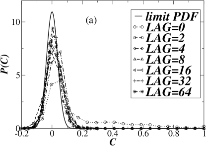
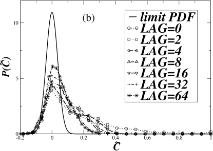
Figure 1: Cross-correlations among the $N=48$ world financial index returns each of size $T=2744$ (a) The empirical pdf of the coefficients of the cross-correlation matrix C calculated between index returns with increasing $\Delta t$ quickly converges to the Gaussian form. The normal distribution is the distribution of the pairwise cross-correlations for finite length uncorrelated time series, which is a normal distribution with mean zero and standard deviation $\frac{1}{\sqrt{T}}$. between (b) The empirical pdf of the coefficients of the matrix $\tilde{\textsf{C}}$ calculated between index volatilities approaches the pdf of the random matrix more slowly than in (a).

In Fig. 1(a) we show the distribution of cross-correlations between zero and non-zero lags. For $\Delta t=0$ the empirical pdf $P(C_{ij})$ of the cross-correlation coefficients $C_{ij}$ substantially deviates from the corresponding pdf $P(W_{ij})$ of a Wishart matrix, implying the existence of equal-time cross-correlations.

In order to determine whether short-range or long-range cross-correlations accurately characterize world financial markets, we next analyze cross-correlations for $(\Delta t\neq 0)$. We find that with increasing $\Delta t$ the form of $P(C_{ij})$ quickly approaches the pdf $P(W_{ij})$, which is normally distributed with zero mean and standard deviation $1/\sqrt{N}$ Shumway .

In Fig. 1(b) we also show the distribution of cross-correlations between magnitudes. In financial data, returns $R_{i,t}$ are generally uncorrelated or short-range auto-correlated, whereas the magnitudes are generally long-range auto-correlated Granger96 ; Liu . We thus examine the cross-correlations $\tilde{C}_{ij}(\Delta t)$ between $|r_{i,t}|$ for different $\Delta t$. In Fig. 1(b) we find that with increasing $\Delta t$, $P(\tilde{C}_{ij})$ approaches the pdf of random matrix $P(W_{ij})$ more slowly than $P(C_{ij})$, implying that cross-correlations between index magnitudes persist longer than cross-correlations between index returns.

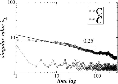
Figure 2: Long-range magnitude cross-correlations. The largest singular value $\lambda_{L}$ obtained from the spectrum of the matrices C and $\tilde{\textsf{C}}$ versus time lag $\Delta t$. With increasing $\Delta t$, the largest singular values obtained for C of returns decays more quickly than $\tilde{\textsf{C}}$ calculated for absolute values of returns. The magnitude cross-correlations decay as a power law function with the scaling exponent of $\approx 0.25$.

In order to demonstrate the decay of cross-correlations with time lags, we apply modified TLRMT. Fig. 2 shows that with increasing $\Delta t$ the largest singular value calculated for $\tilde{\textsf{C}}$ decays more slowly than the largest singular value calculated for C. This result implies that among world indices, the cross-correlations between magnitudes last longer than cross-correlations between returns. In Fig. 2 we find that $\lambda_{L}$ vs. $\Delta t$ decays as a power law function with the scaling exponent equal to 0.25. The faster decay of $\lambda_{L}$ vs. $\Delta t$ for C implies very weak (or zero) cross-correlations among world-index returns for larger $\Delta t$, which agrees with the empirical finding that world indices are often uncorrelated in returns. Our findings of long-range cross-correlations in magnitudes among the world indices is, besides a finding in Ref. Solnik96 , another piece of “bad news” for international investment managers. World market risk decays very slowly. Once the volatility (risk) is transmitted across the world, the risk lasts a long time.

IV Global Factor Model

The arbitrage pricing theory states that asset returns follow a linear combination of various factors Ross . We find that the factor structure can also model time lag pairwise cross-correlations between the returns and between magnitudes. To simplify the structure, we model the time lag cross-correlations with the assumption that each individual index fluctuates in response to one common process, the “global factor” $M_{t}$,

$$R_{i,t}=\mu_{i}+b_{i}M_{t}+\epsilon_{i,t}.$$ (8)

Here in the global factor model (GFM), $\mu_{i}$ is the average return for index $i$, $M_{t}$ is the global factor, and $\epsilon_{i,t}$ is the linear regression residual, which is independent of $M_{t}$, with mean zero and standard deviation $\sigma_{i}$. Here $b_{i}$ indicates the covariance between $R_{i,t}$ and $M_{t}$, ${\rm Cov}(R_{i,t},M_{t})=b_{i}{\rm Var}(M_{t})$. This single factor model is similar to the Sharpe market model Sharpe63 , but instead of using a known financial index as the global factor $M_{t}$, we use factor analysis to find $M_{t}$, which we introduce in the next section. We also choose $M_{t}$ as a zero-mean process, so the expected return $E(R_{i,t})=\mu_{i}$, and the global factor $M_{t}$ is only related with market risk. We define a zero-mean process $r_{i,t}$ as

$$r_{i,t}\equiv R_{i,t}-E(R_{i,t})=b_{i}M_{t}+\epsilon_{i,t}.$$ (9)

A second assumption is that the global factor can account for most of the correlations. Therefore we can assume that there are no correlations between the residuals of each index, ${\rm Cov}(\epsilon_{i,t},\epsilon_{j,t})=0$. Then the covariance between $R_{i,t}$ and $R_{j,t}$ is

$${\rm Cov}(R_{i,t},R_{j,t})={\rm Cov}(r_{i,t},r_{j,t})=b_{i}b_{j}{\rm Var}(M_{t}).$$ (10)

The covariance between magnitudes of returns depends on the return distribution of $M_{t}$ and $R_{i,t}$, but the covariance between squared magnitudes $r_{i,t}^{2}$ indicates the properties of the magnitude cross-correlations. The covariance between $r_{i,t}^{2}$ and $r_{j,t}^{2}$ is

$${\rm Cov}(r_{i,t}^{2},r_{j,t}^{2})=b_{i}^{2}b_{j}^{2}{\rm Var}(M_{t}^{2}).$$ (11)

The above results in Eqs. (10)-(11) show that the variance of the global factor and square of the global factor account for all the zero time lag covariance between returns and squared magnitudes. For time lag covariance between $r_{i,t}$, we find

$${\rm Cov}(r_{i,t},r_{j,t},\Delta t) = E(r_{i,t},r_{j,t-\Delta t})-E(r_{i,t})E(r_{j,t-\Delta t})$$ (12)

$$= b_{i}b_{j}A_{M}(\Delta t).$$ (13)

Here

$$A_{M}(\Delta t)\equiv E(M_{t}M_{t-\Delta t})-E(M_{t})E(M_{t-\Delta t})$$ (14)

is the autocovariance of $M_{t}$. Similarly, we find

$${\rm Cov}(r_{i,t}^{2},r_{j,t}^{2},\Delta t)=b_{i}^{2}b_{j}^{2}A_{M^{2}}(\Delta t).$$ (15)

Here

$$A_{M^{2}}(\Delta t)=E(M_{t}^{2}M_{t-\Delta t}^{2})-E(M_{t}^{2})E(M_{t-\Delta t}^{2})$$ (16)

is the autocovariance of $M_{t}^{2}$.

In GFM, the time lag covariance between each pair of indices is proportional to the autocovariance of the global factor. For example, if there is short-range autocovariance for $M_{t}$ and long-range autocovariance for $M_{t}^{2}$, then for individual indices the cross-covariance between returns will be short-range and the cross-covariance between magnitudes will be long-range. Therefore, the properties of time-lag cross-correlation in multiple time series can be modeled with a single time series— the global factor $M_{t}$.

The relationship between time lag covariance among two index returns and autocovariance of the global factor also holds for the relationship between time lag cross-correlations among two index returns and auto-correlation function of the global factor, because it only need to normalize the original time series to mean zero and standard deviation one.

V Estimation and Analysis of the Global Factor

V.1 Estimation of the Global factor

In contrast to domestic markets, where for a given country we can choose the stock index as an estimator of the “global” factor, when we study world markets the global factor is unobservable. At the world level when we study cross-correlations among world markets, we estimate the global factor using principal component analysis (PCA) Jolliffe86 .

In this section we use bold font for N dimensional vectors or $N\times N$ matrix, and underscore $t$ for time series. Suppose ${\bf R_{t}}\equiv(R_{1,t},R_{2,t},\ldots,R_{N,t})^{T}$ is the multiple time series, each row of which is an individual time series $R_{i,t}=(R_{i,1},R_{i,2},\ldots,R_{i,T})$. We standardize each time series to zero mean and standard deviation 1 as

$$z_{i,t}\equiv\frac{R_{i,t}-\langle R_{i,t}\rangle}{\sigma(R_{i,t})}.$$ (17)

The correlation matrix can be calculated as ${\bf C}\equiv\frac{1}{T}{\bf z_{t}}{\bf z_{t}}^{T}$ where ${\bf z_{t}}^{T}$ is the transpose of ${\bf z_{t}}$, and the $T$ in the denominator is the length of each time series. Then we diagonalize the $N\times N$ correlation matrix ${\bf C}$

$${\bf C}={\bf U}{\bf\Lambda}{\bf U}^{T}.$$ (18)

Here ${\bf\Lambda}\equiv{\rm diag}(\lambda_{1},\lambda_{2},...,\lambda_{N})$ and $\lambda_{1}\geq\lambda_{2}\geq...\geq\lambda_{N}$ are the eigenvalues in non-increasing order, ${\bf U}$ is an orthonormal matrix, whose $i$-th column is the basis eigenvector ${\bf u_{i}}$ of ${\bf C}$, and ${\bf U}^{\bf T}$ is the transpose of ${\bf U}$, which is equal to ${\bf U}^{-1}$ because of orthonormality.

For each eigenvalue and the corresponding eigenvector, it holds

$$\lambda_{i}={\bf u_{i}}^{T}{\bf C}{\bf u_{i}}={\bf u_{i}}^{T}{\rm Cov}({\bf z_{t}}){\bf u_{i}}={\rm Var}({\bf u_{i}}^{T}{\bf z_{t}})={\rm Var}({\alpha}_{i,t}).$$ (19)

According to PCA, ${\alpha_{i,t}}={\bf u_{i}}^{T}{\bf z_{t}}$ is defined as the $i$-th principal component ($\alpha_{i,t}$), and the eigenvalue $\lambda_{i}={\rm Var}({z_{i,t}})$ indicates the portion of total variance of ${\bf z_{t}}$ contributed to ${\alpha_{i,t}}$, as shown in Eq. (19). Since the total variance of ${\bf z_{t}}$ is

$$\sum_{i=1}^{N}{\rm Var}({z_{i,t}})={\rm trace}({\bf C})=\sum_{i=1}^{N}\lambda_{i},$$ (20)

the expression $\lambda_{i}/{\rm trace}({\bf C})$ indicates the percentage of the total variance of ${\bf z_{t}}$ that can be explained by the ${\alpha_{i,t}}$. According to PCA (a) the principal components ${\alpha_{i,t}}$ are uncorrelated with each other and (b) ${\alpha_{i,t}}$ maximizes the variance of the linear combination of ${\bf U}^{T}{\bf z_{t}}$ with the orthonormal restriction ${\bf U}^{T}{\bf U}=1$ given the previous principal components Jolliffe86 .

From the orthonormal property of ${\bf U}$ we obtain

$${\bf I} = {\bf UU}^{T}={\bf u}_{1}{\bf u}_{1}^{T}+{\bf u}_{2}{\bf u}_{2}^{T}+...+{\bf u}_{N}{\bf u}_{N}^{T},$$ (21)

where I is the identity matrix. Then the multiple time series ${\bf z_{t}}$ can be represented as a linear combination of all the $\boldsymbol{\alpha_{t}}$

$${\bf z_{t}} = ({\bf u}_{1}{\bf u}_{1}^{T}+{\bf u}_{2}{\bf u}_{2}^{T}+...+{\bf u}_{N}{\bf u}_{N}^{T}){\bf z_{t}}$$ (22)

$$= {\bf u}_{1}{\alpha_{1,t}}+{\bf u}_{2}\alpha_{2,t}+...+{\bf u}_{N}\alpha_{N,t}.$$

The total variance of all time series can be proved to be equal to the total variance of all principal components

$$\sum_{i=1}^{N}{\rm Var}({z}_{i,t}) = {\rm Var}({\bf u}_{1}){\alpha_{1,t}}+...+{\rm Var}({\bf u}_{N})\alpha_{N,t}$$ (23)

$$= \sum_{i=1}^{N}{\bf u}_{i}^{T}{\bf u}_{i}{\rm Var}(\alpha_{i,t})=\sum_{i=1}^{N}{\rm Var}(\alpha_{i,t}).$$ (24)

Next we assume that ${\rm Var}({\alpha_{1,t}})=\lambda_{1}$ is much larger than each of the rest of eigenvalues—which means that the first $\boldsymbol{\alpha_{t}}$, ${\alpha}_{1,t}$, accounts for most of the total variances of all the time series. We express ${\bf z_{t}}$ as the sum of the first part of Eq. (22) corresponding to ${\alpha_{1,t}}$ and the error term combined from all other terms in Eq. (22). Thus

$${\bf z_{t}} = {\bf u}_{1}{\alpha_{1,t}}+{\boldsymbol{\eta_{t}}},$$

$${\boldsymbol{\eta_{t}}} \equiv \sum_{i=2}^{N}{\bf u}_{i}\alpha_{i,t}.$$ (25)

Then ${\alpha_{1,t}}$ is a good approximation of the global factor $M_{t}$, because it is a linear combination of $R_{i,t}$ that accounts for the largest amount of the variance. ${\alpha_{1}}$ is a zero-mean process because it is a linear combination of ${z}_{i,t}$ which are also zero-mean processes (see Eq. (17)).

Comparing Eqs. (17) and (25) with

$$R_{i,t}=\mu_{i}+b_{i}M_{t}+\epsilon_{i,t},$$ (26)

we find the following estimates:

$$M_{t} = {\alpha_{1,t}},$$

$$b_{i} = \sigma(R_{i})u_{1i},$$

$$\epsilon_{i,t} = \sigma(R_{i})\eta_{i,t}.$$ (27)

Using Eq. (19) we find that

$${\rm Corr}(M_{t},R_{i,t})=\sqrt{\lambda_{i}}u_{i1}.$$ (28)

In the rest of this work, we apply the method of Eq. (27) to empirical data.

V.2 Analysis of the global factor

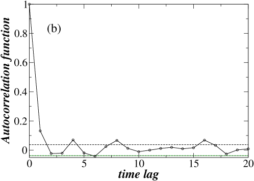
Figure 3: Short-range cross-correlations of a global factor. (a) Time series of the global factor. (b) The auto-correlation function (ACF) of the global factor. The region between dashed lines is the 95% confidence interval for the no auto-correlation hypothesis. Auto-correlations are smaller than 0.132 except $\Delta t=0$, and become insignificant after time lag $\Delta t=2$, with no more than one significant auto-correlation for every 20 time lags. Therefore, only short-range auto-correlations can be found in the global factor.

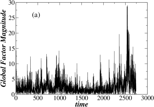
Figure 4: Long-range cross-correlations of the magnitude global factor.(a) Time series of magnitudes of the global factor. (b) Auto-correlations of magnitudes of the global factor. The region between dashed lines is the 95% confidence interval for the no auto-correlation hypothesis. Auto-correlations are much larger than the auto-correlations of the global factor itself, is as large as 0.359 at $\Delta t=2$, and is still larger than 0.2 until $\Delta t=33$. For every time lag, the autocorrelation is significant even after $\Delta t=100$. Therefore long-range auto-correlations exist in the magnitudes of the global factor.

Next we apply the method of Eq. (27) to estimate the global factor of 48 world index returns. We calculate the auto-correlations of $M_{t}$ and $|M_{t}|$, which are shown in Figs. 3 and 4. Precisely, for the world indices, Fig. 3(a) shows the time series of the global factor $M_{t}$, and Fig. 3(b) shows the auto-correlations in $M_{t}$. We find only short-range auto-correlations because, after an interval $\Delta t=2$, most auto-correlations in $M_{t}$ fall in the range of $(-1.96\sqrt{1/T},1.96\sqrt{1/T})$ Shumway , which is the 95% confidence interval for zero auto-correlations, Here $T=2744$.

For the 48 world index returns, Fig. 4(a) shows the time series of magnitudes $|M_{t}|$, with few clusters related to market shocks during which the market becomes fluctuates more. Fig. 4(b) shows that, in contrast to $M_{t}$, the magnitudes $|M_{t}|$ exhibit long-range auto-correlations since the values $|M_{t}|$ are significant even after $\Delta t=100$. The auto-correlation properties of the global factor are the same as the auto-correlation properties of the individual indices, i.e., there are short-range auto-correlations in $M_{t}$ and long-range power-law auto-correlations in $|M_{t}|$ Granger96 ; Liu . These results are also in agreement with Fig. 1(b) where the largest singular value $\lambda_{L}$ vs. $\Delta t$ calculated for $\tilde{\textsf{C}}$ decays more slowly than the largest singular value calculated for C. As found in Ref. Podobnik10 for $\Delta t>>1$, $\lambda_{L}(\Delta t)$ approximately follows the same decay pattern as cross-correlation functions. Although a Ljung-Box test shows that the return auto-correlation is significant for a 95% confidence level LBtest , the return auto-correlation is only 0.132 for $\Delta t=1$ and becomes insignificant after $\Delta t=2$ . Therefore, for simplicity, we only consider magnitude cross-correlations in modeling the global factor.

We model the long-range market-factor returns M with a particular version of the GARCH process, the GJR GARCH process Glosten , because this GARCH version explains well the asymmetry in volatilities found in many world indices Glosten ; Rossiter ; Joel10 . The GJR GARCH model can be written as

$$\epsilon_{t} = \sigma_{t}\eta_{t},$$ (29)

$$\sigma^{2}_{t} = \alpha_{0}+\sum_{i=1}^{q}(\alpha_{i}+\gamma T_{t-i})\epsilon_{t-i}^{2}+\sum_{i=1}^{p}\beta_{i}\sigma^{2}_{t-i},$$ (30)

where $\sigma_{t}$ is the volatility and $\eta_{t}$ is a random process with a Gaussian distribution with standard deviation 1 and mean 0. The coefficients $\alpha$ and $\beta$ are determined by a maximum likelihood estimation (MLE) and $T_{t}=1$ if $\epsilon_{t-1}<0$, $T_{t}=0$ if $\epsilon_{t-1}\geq 0$. We expect the parameter $\gamma$ to be positive, implying that “bad news” (negative increments) increases volatility more than “good news”. For the sake of simplicity, we follow the usual procedure of setting $p=q=1$ in all numerical simulations. In this case, the GJR-GARCH(1,1) model for the market factor can be written as

$$M_{t} = \sigma_{t}\eta_{t},$$ (31)

$$\sigma^{2}_{t} = \alpha_{0}+(\alpha_{1}+\gamma T_{t-1})\epsilon_{t-1}^{2}+\beta_{1}\sigma^{2}_{t-1}.$$ (32)

We estimate the coefficients in the above equations using MLE, where the estimated coefficients are shown in Table. 1.

Next we test the hypothesis that a significant percentage of the world cross-correlations can be explained by the global factor. By using PCA we find that the global factor can account for 30.75% of the total variance. Note that, according to RMT, only the eigenvalues larger than the largest eigenvalue of a Wishart matrix calculated by Eq. (3) (and the corresponding $\boldsymbol{\alpha}$s) are significant. To calculate the percentage of variance the significant $\boldsymbol{\alpha}$s account for, we employ the RMT approach proposed in Ref. prl . The largest eigenvalue for a Wishart matrix is $\lambda_{+}=1.282$ for $N=48$ and $T=2744$ we found in the empirical data. From all the 48 eigenvalues, only the first three are significant: $\lambda_{1}=14.762$, $\lambda_{2}=3.453$, and $\lambda_{3}=1.380$. This result implies that among the significant factors, the global factor accounts for $\lambda_{1}/\sum_{i=1}^{3}\lambda_{i}=75.34\%$ of the variance, confirming our hypothesis that the global factor accounts for most variance of all individual index returns.

PCA is defined to estimate the percentage of variance the global factor can account for zero time lag correlations. Next we study the time lag cross-correlations after removing the global trend, and apply the SVD to the correlation matrix of regression residuals $\eta_{i}$ of each index [see Eq. (8)]. Our results show that for both returns and magnitudes, the remaining cross-correlations are very small for all time lags compared to cross-correlations obtained for the original time series. This result additionally confirms that a large fraction of the world cross-correlations for both returns and magnitudes can be explained by the global factor.

VI Applications of Global Factor Model

VI.1 Locating and Forecasting global risks

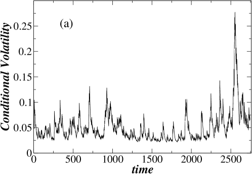
Figure 5: (a) Conditional volatility of the global factor, showing that the clusters in the conditional volatilities may serve to predict market crashes. In each cluster, the height indicates the size of the market crash, and the width indicates its duration. (b) The 100-day forecasted volatility of the global factor, using the past data ranging from 4 Jan 1999 through 10 July 2009. It will converge to the unconditional volatility asymptotically.

The asymptotic (unconditional) variance for the GJR-GARCH model is $\alpha_{0}/(1-\alpha_{1}-\beta_{1}-\gamma/2)=10.190$ Ling . For the market factor the conditional volatility $\sigma_{t}$ can be estimated by recursion using the historical conditional volatilities and fitted coefficients in Eq. (32). For example, the largest cluster at the end of the graph shows the 2008 financial crisis. In Fig. 5(a) we show the time series of the conditional volatility of Eq. (32) of the global factor. The clusters in the conditional volatilities may serve to predict market crashes. In each cluster, the height is a measure of the size of the market crash, and the width indicates its duration. In Fig. 5(b) we show the forecasting of the conditional volatility of the global factor, which asymptotically converges to the unconditional volatility.

VI.2 Finding uncorrelated individual indices

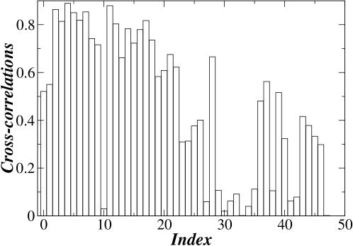
Figure 6: Cross-correlation between the global factor $M_{t}$ and each individual index $R_{i,t}$, $i=1,2,...,48$. The global factor has large correlation with most of the indices. However, there are indices that are not much correlated with the global factor. 10 of the 48 indices have a correlation smaller than 0.1 between the global factor, corresponding to the indices for Iceland, Malta, Nigeria, Kenya, Israel, Oman, Qatar, Pakistan, Sri Lanka, and Mongolia. Hence, unlike most countries, the economies of these 10 countries are more independent of the world economy.

Next, in Fig. 6 we show the cross-correlations between the global factor and each individual index using Eq. (28). There are indices for which cross-correlations with the global factor are very small compared to the other indices; 10 of 48 indices have cross-correlations coefficients with the global factor smaller than 0.1. These indices correspond to Iceland, Malta, Nigeria, Kenya, Israel, Oman, Qatar, Pakistan, Sri Lanka, and Mongolia. The financial market of each of these countries is weakly bond with financial markets of other countries. This is useful information for investment managers because one can reduce the risk by investing in these countries during world market crashes which, seems, do not severely influence these countries.

VII Discussion

We have developed a modified time lag random matrix theory (TLRMT) in order to quantify the time-lag cross-correlations among multiple time series. Applying the modified TLRMT to the daily data for 48 world-wide financial indices, we find short-range cross-correlations between the returns, and long-range cross-correlations between their magnitudes. The magnitude cross-correlations show a power law decay with time lag, and the scaling exponent is 0.25. The result we obtain, that at the world level the cross-correlations between the magnitudes are long-range, is potentially significant because it implies that strong market crashes introduced at one place have an extended duration elsewhere—which is “bad news” for international investment managers who imagine that diversification across countries reduces risk.

We model long-range world-index cross-correlations by introducing a global factor model in which the time lag cross-correlations between returns (magnitudes) can be explained by the auto-correlations of the returns (magnitudes) of the global factor. We estimate the global factor as the first component by using principal component analysis. Using random matrix theory, we find that only three principal components are significant in explaining the cross-correlations. The global factor accounts for 30.75% of the total variance of all index returns, and 75.34% of the variance of the three significant principle components. Therefore, in most cases, a single global factor is sufficient.

We also show the applications of the GFM, including locating and forecasting world risk, and finding individual indices that are weakly correlated to the world economy. Locating and forecasting world risk can be realized by fitting the global factor using a GJR-GARCH(1,1) model, which explains both the volatility correlations and the asymmetry in the volatility response to both “good news” and “bad news.” The conditional volatilities calculated after fitting the GJR-GARCH(1,1) model indicates the global risk, and the risk can be forecasted by recursion using the historical conditional volatilities and the fitted coefficients. To find the indices that are weakly correlated to the world economy, we calculate the correlation between the global factor and each individual index. We find 10 indices which have a correlation smaller than 0.1, while most indices are strongly correlated to the global factor with the correlations larger than 0.3. To reduce risk, investment managers can increase the proportion of investment in these countries during world market crashes, which do not severely influence these countries.

Based on principal component analysis, we propose a general method which helps extract the most significant components in explaining long-range cross-correlations. This makes the method suitable for broad range of phenomena where time series are measured, ranging from seismology and physiology to atmospheric geophysics. We expect that the cross-correlations in EEG signals are dominated by the small number of most significant components controlling the cross-correlations. We speculate that cross-correlations in earthquake data are also controlled by some major components. Thus the method may have significant predictive and diagnostic power that could prove useful in a wide range of scientific fields.

We thank Ivo Grosse and T. Preis for valuable discussions and NSF for financial support.

Table 1: GJR-GARCH(1,1) coefficients of the global factor. The P-values and t-values comfirms that all these parameters are significant at 95% confidence level. The positive value of $\gamma$ means “bad news” has larger impact on the global market than “good news”. We find $\alpha_{1}+\beta_{1}+\gamma/2=0.9756$, which is very close to 1, and so indicate long-range volatility auto-correlations.

	Value	Std.Error	t-value	P-value
$\alpha_{0}$	0.2486	0.0283	8.789	0.0000
$\alpha_{1}$	0.0170	0.0080	2.128	0.0334
$\beta_{1}$	0.8790	0.0101	86.939	0.0000
$\gamma$	0.1591	0.0148	10.805	0.0000

References

- (1) R. A. Meyers, ed., Encyclopedia of Complexity and Systems Science (Springer, 2009).
- (2) K. Christensen and N. R. Moloney, Complexity and Criticality (Imperial College Press, 2010).
- (3) R. Cohen and S. Havlin, Complex Networks: Structure, Robustness and Function (Cambridge University Press, 2010).
- (4) Heartbeat interval time series are among many time series characterizing the functioning human.
- (5) P. Samuelsson, E. V. Sukhorukov, and M. Buttiker, Phys. Rev. Lett. 91, 157002 (2003).
- (6) A. Cottet, W. Belzig, and C. Bruder, Phys. Rev. Lett. 92, 206801 (2004).
- (7) I. Neder, M. Heiblum, D. Mahalu, and V. Umansky, Phys. Rev. Lett. 98, 036803 (2007).
- (8) K. Yamasaki, A. Gozolchiani, and S. Havlin, Phys. Rev. Lett. 100, 228501 (2008).
- (9) A. Corral, Phys. Rev. Lett. 95, 159801 (2005).
- (10) M. Campillo and A. Paul, Science 299, 547 (2003).
- (11) E. Lippiello, L. de Arcangelis, and C. Godano, Phys. Rev. Lett. 100, 038501 (2008).
- (12) B. Solnik, C. Bourcrelle, and Y. Le Fur, Fin. Anal. Journal 52, 17–34 (1996).
- (13) C. B. Erb, C. R. Harvey, and T. E. Viscanta, Fin. Analysts Journal 50, 32–45 (1994).
- (14) B. LeBaron, W.B. Arthur, R. Palmer, J. Econ. Dyn. Control 23, 1487 (1999)
- (15) L. Laloux et al., Phys. Rev. Lett. 83, 1467-1470 (1999); V. Plerou et al., ibid. 83, 1471–1474 (1999); Phys. Rev. E 65, 066126 (2002).
- (16) M. Takayasu and H. Takayasu, Statistical Physics and Economics (Cambridge University Press, Cambridge, 2010).
- (17) R. N. Mantegna, Eur. Phys. J. B 11, 193 (1999).
- (18) L. Kullmann, J. Kertesz and K. Kaski, Phys. Rev. E 66, 026125 (2002).
- (19) M. Tumminello, T. Aste, T. Di Matteo and R. N. Mantegna, Proc. Natl. Acad. Sci. USA 102, 10421 (2005).
- (20) T. Mizuno, H. Takayasu and M. Takayasu, Physica A 364, 336 (2006).
- (21) B. Podobnik and H. E. Stanley, Phys. Rev. Lett. 100, 084102 (2008); Podobnik B. et al., Proc. Natl. Acad. Sci. USA 106, 22079 (2009).
- (22) S. Arianos and A. Carbone, J. Stat. Mech. P03037 (2009).
- (23) B. Podobnik et al., European Phys. Journal B 56, 47 (2007).
- (24) H. M. Markowitz, J. Finance 7, 77 (1952).
- (25) P. Bob, M. Susta, K. Glaslova and N. N. Boutros, Psychiatry Research 177, 37 (2010).
- (26) B. Podobnik et al., Europhys. Lett. 90, 68001 (2010).
- (27) I. T. Jolliffe, Principal Component Analysis (Springer-Verlag, New York, 1986).
- (28) T. Guhr and B. Kalber, J. Phys. A 36, 3009 (2003).
- (29) C. K. Peng et al Phys. Rev. E 49, 1685 (1994); A. Carbone, G. Castelli, and H. E. Stanley, Physica A 344, 267 (2004); L. Xu et al, Phys. Rev. E 71, 051101 (2005); A. Carbone, G. Castelli, and H. E. Stanley, Phys. Rev. E 69, 026105 (2004).
- (30) G. E. P. Box and G. M. Jenkins, Time Series Analysis, Forecasting and Control (Holden-Day, San Francisco, 1970).
- (31) R. F. Engle, Econometrica 50, 987 (1982).
- (32) T. Bollerslev, J. Econometrics 31, 307 (1986).
- (33) Z. Ding and C. W. J. Granger, J. Econometrics 73, 185 (1996).
- (34) Y. Ashkenazy et al., Phys. Rev. Lett. 86, 1900 (2001).
- (35) J. W. Kantelhardt et al., Phys. Rev. E 65, 051908 (2002).
- (36) V. N. Livina et al., Phys. Rev. E 67, 042101 (2003).
- (37) B. Podobnik et al., Phys. Rev. E Rapid Communication 71, 025104(R) (2005).
- (38) W. F. Sharpe, Journal of Finance 19, 425 (1964).
- (39) W. F. Sharpe, Portfolio theory and capital markets (McGraw-Hill, New York, 1970).
- (40) T. Bollerslev, R. F. Engle, and J. M. A. Wooldridge, The Review of Economics and Statistics 72, 498 (1988).
- (41) T. Bollerslev, J. Political Economy 96, 116 (1990).
- (42) R. Engle and F. K. Kroner, Econometric Theory 11, 122 (1995).
- (43) G. Canarella and S. K. Pollard, Int. Rev. of Economics 54, 445 (2007).
- (44) Z. Ding, C. W. J. Granger, and R. F. Engle, J. Empirical Finance 1, 83 (1993).
- (45) FTSE 100, DAX, CAC 40, IBEX 35, Swiss Market, FTSE MIB, PSI 20, Irish overall, OMX Iceland 15, AEX, BEL 20, Luxembourg LuxX, OMX Copenhagen 20, OMX Helsinki, OBX Stock, OMX Stockholm 30, Austrian Traded ATX, Athex Composite Share Price, WSE WIG, Prague Stock Exch, Budapest Stock Exch INDX, Bucharest BET Index, SBI20 Slovenian Total Mt, OMX Tallin OMXT, Malta Stock Exchange IND, FTSE/JSE Africa TOP40 IX
- (46) ISE National 100, Tel Aviv 25, msm30, dsm 20, Mauritius Stock Exchange, NIKKEI 225, Hang Seng, Shanghai se b share, all Ordinaries, nzx all, Karachi 100, Sri Lanka Colombo all sh, Stock Exch Of Thai, Jakarta Composite, FTSE Bursa Malaysia KLCI, PSEi - Philippine SE, MSE Top 20
- (47) S&P 500, Mexico BOLSA
- (48) FTSE/JSE Africa TOP40 IX, CFG 25, Nigerian Stock Exchange All Shares, Nairobi Stock Exchange 20-Share
- (49) F. Longin and B. Solnik, J. International Money and Finance 14, 3 (1995).
- (50) L. Ramchand and R. Susmel, J. Empirical Finance 5, 397 (1998).
- (51) M. L. Mehta, Random Matrices (Academic Press, Boston, 1991).
- (52) T. Guhr, A. Müller-Groeling, and H. Weidenmüller, Physics Reports 299, 190 (1998).
- (53) L. Laloux, P. Cizeau, J.-P. Bouchaud, and M. Potters, Risk 12, 69 (1999).
- (54) A. Utsugi, K. Ino, and M. Oshikawa, Phys. Rev. E 70, 026110 (2004).
- (55) R. K. Pan and S. Sinha, Phys. Rev. E 76, 046116 (2007).
- (56) J. Shen and B. Zheng, Europhys. Lett. 86, 48005 (2009).
- (57) M. Potters et al., Acta Phys. Polonica B 36, 2767 (2005).
- (58) J. Kwapien et al., Acta Phys. Polonica B 37, 3039 (2006).
- (59) J.-P. Bouchaud et al., Eur. Phys. J. B 55, 201 (2007).
- (60) A. M. Sengupta and P. P. Mitra, Phys. Rev. E 60, 3389 (1999).
- (61) R. H. Shumway and D. S. Stoffer, Time Series Analysis and Its Applications (Springer-Verlag, New York, 2000).
- (62) Y. Liu et al. Physica A 245, 437 (1997); Phys. Rev. E 60, 1390 (1999); P. Cizeau et al., Physica A 245, 441 (1997).
- (63) S. A. Ross, J. Economic Theory 13, 341 (1976).
- (64) W. F. Sharpe, Management Science 9, 277 (1963).
- (65) G. M. Ljung and G. E. P. Box, Biometrika 65, 297 (1978).
- (66) L. Glosten, R. Jagannathan, and D. Runkle, J. Finance 48, 1779 (1993).
- (67) R. Rossiter and S. A. Jayasuriya, J. Int. Finance and Eco. 8, 11 (2008).
- (68) J. Tenenbaum et al., Phys. Rev. E 82, 046104 (2010).
- (69) S. Ling and M. McAleer, J. Econometrics 106, 109 (2002).