A simple model for the dynamical Casimir effect for a static mirror with time-dependent properties

Abstract

We consider a real massless scalar field in 1+1 dimensions satisfying time-dependent Robin boundary condition at a static mirror. This condition can simulate moving reflecting mirrors whose motions are determined by the time-dependence of the Robin parameter. We show that particles can be created from vacuum, characterizing in this way a dynamical Casimir effect.

I Introduction

The phenomenon of particle creation from quantum vacuum by moving boundaries or due to time-dependent properties of materials, commonly referred to as the dynamical Casimir effect (DCE) Yablo-1989 ; Schwinger-1992 , has been investigated since the pioneering works of Moore Moore-JMP-1970 and DeWitt DeWitt-1975 (see also the subsequent works carried in Refs. others ) in a wide variety of situations and with the aid of quite different approaches (see Refs. Reviews-I for excellent reviews on the subject). Particularly, perturbative and numerical approaches were applied for single mirrors Single-mirror ; Jaekel-PRL-1996 ; Mintz-JPA-2006 ; Mintz-JPA-2006-2 and cavities Cavities . Initial field states different from vacuum were also considered for single mirrors temperatura-uma-fronteira ; equivalencia-DN and cavities as well temperatura-cavidade . The first experimental observation of this phenomenon was recently announced in Ref. Wilson-arXiv .

Taking into account the difficulties in generating appreciable mechanical oscillation frequencies (of the order of GHz) to obtain a detectable number of photons, recent experimental schemes focus on simulating moving boundaries by considering material bodies with time-dependent electromagnetic properties. These possibilities were first proposed by Yablonovitch Yablo-1989 and have been further developed in theoretical works which considered materials with time-dependent permittivities and time-dependent surface conductivities time-dependent-prop ; Crocce-PRA-2004 ; Naylor-PRA-2009 (see the nice compilation done in Ref. Naylor-PRA-2009 ). For instance, in Ref. Crocce-PRA-2004 the DCE for a massless scalar field within a cavity containing a thin semiconducting film with time-dependent conductivity and centered at the middle of the cavity was studied. The coupling of such a film to the quantum scalar field was modeled by a delta-potential with time-dependent strength. A generalization to the case of an electromagnetic field was carried out in Naylor-PRA-2009 . Very promising and ingenious experimental set-ups to simulate non-stationary boundaries include the changing of the reflectivity of a semiconductor by the incidence of a periodic sequence of short laser pulses Experimento-MIR or by using a coplanar waveguide terminated by a superconducting quantum interference device (SQUID). Applying a variable magnetic flux on the SQUID, a single moving mirror can be simulated Johansson ; Nation . A first step toward the experimental verification of the DCE was recently made in Wilson-PRL-2010 using this approach. Moreover, the same group recently claimed to have observed the DCE Wilson-arXiv .

Key ingredients in the predictions of the DCE are the boundary conditions (BC) under consideration and naturally the quantum field submitted to those BC. Quite general BC are the so called Robin ones which, for the case of a scalar field in 1+1 dimensions and a single mirror fixed at $x=a$, are defined by $\phi(t,x=a)=\gamma[\partial_{x}\phi(t,x)]_{x=a}$, where $\gamma$ is a real parameter (called hereafter as Robin parameter). For the case of a moving boundary, the previous relation is imposed in the comoving frame and the corresponding BC in the laboratory frame is obtained after an appropriate Lorentz transformation.

This BC have the nice feature of interpolating continuously Dirichlet ($\gamma\rightarrow 0$) and Neumann ($\gamma\rightarrow\infty$) ones and occurs in several areas of physics and mathematics. For instance, in classical mechanics they will appear if one considers a vibrating string coupled to a spring which satisfies Hooke’s law and is localized at one of its edges Mintz-JPA-2006 ; Mintz-JPA-2006-2 ; Robin-CM . In non-relativistic quantum mechanics, Robin BC occur as the most general BC imposed by a wall ensuring the hermiticity of the hamiltonian as well as a null probability flux through it Robin-QM . Regarding the static Casimir effect Casimir-1948 , it was shown that the Casimir force between two parallel plates which impose Robin BC on a real scalar field may have its sign changed if appropriate choices are made for the corresponding Robin parameters of each mirror Romeo-JPA-2002 . Such kind of repulsive Casimir force was also predicted, in the case of parallel plates, by Boyer in the 70s, who considered a pair of perfectly conducting and infinitely permeable plates Boyer-PRA-1974 . Further investigations on the influence of Robin BC in the static Casimir effect, including thermal corrections and the case of Casimir piston setups, were carried, for instance, in Refs. Robin-SCE . See also Refs. Quantum-Vacuum for the influence of this BC on the structure of quantum vacuum.

Only recently Robin BC were considered in the context of the DCE. For a massless scalar field in 1+1 dimensions submitted to a Robin BC at a single moving mirror the radiation reaction force on the moving mirror and the particle creation rate were computed in Refs. Mintz-JPA-2006 ; Mintz-JPA-2006-2 . Interestingly, for Robin BC, the radiation reaction force acquires a dispersive component, in sharp contrast with Dirichlet and Neumann cases where the force is purely dissipative. It was also shown that, for a given Robin parameter, there exists a mechanical frequency of motion that dramatically reduces the particle creation effect Mintz-JPA-2006-2 . Finally, and of crucial importance for the present work, Robin BC can also be useful to describe phenomenological models for penetrable surfaces and under certain conditions they simulate the plasma model for real metals Robin-EM . In these situations, for frequencies $\omega$ much smaller than the plasma frequency $\omega_{\mbox{\footnotesize{P}}}$, the Robin parameter $\gamma$ can be identified as the plasma wavelength $\lambda_{\mbox{\footnotesize{P}}}$. In other words, the Robin parameter $\gamma$ gives us an estimative of the penetration length of the mirror under consideration .

Since to simulate a motion of a reflecting mirror is equivalent to simulate a real metal with time-dependent plasma wavelength, the above interpretation of $\gamma$ leads naturally to the consideration of time-dependent Robin parameters. Specifically speaking, it is quite natural to simulate the motion of a reflecting mirror by considering the quantum field submitted to a Robin BC at a static mirror but with a time-dependent Robin parameter $\gamma(t)$. The kind of boundary motion which is being simulated is determined by the kind of time-dependence of $\gamma(t)$. The purpose of this paper is precisely to analyze this situation for a massless scalar field in 1+1 dimensions. Particularly, we shall compute explicitly the particle creation rate for a natural choice of time-dependence for $\gamma(t)$ which is directly related to recent experimental proposals. This paper in organized as follows: in Sec. II the Bogoliubov transformation between the in and out creation/annihilation operators are obtained, allowing us to find the spectral distribution of the created particles and the particle creation rate in Sec. III and IV, respectively. Finally, in Sec. V we present our conclusions and final remarks. Throughout this work we consider $\hbar=c=1$.

II The Bogoliubov transformation

We start considering a real massless scalar field $\phi$ in 1+1 dimensions which satisfies the Klein-Gordon equation, $\partial^{2}\phi=0$, and is submitted to a time-dependent Robin BC at a mirror fixed at the origin, namely, $\gamma(t)\partial\phi/\partial x|_{x=0}-\phi(0,t)=0$. For simplicity, we assume that $\gamma(t)$ departs only slightly from a positive constant $\gamma_{0}$, so that we can write $\gamma(t)=\gamma_{0}+\delta\gamma(t)$, where $\delta\gamma(t)$ is a smooth time-dependent function satisfying the condition $\max|\delta\gamma(t)|\ll\gamma_{0}$, for every $t$. Under these assumptions in the limit $\gamma_{0}\rightarrow\infty$ we recover Neumann BC. On the other hand, to reobtain Dirichlet BC ($\gamma_{0}\rightarrow 0$), because of condition $\max|\delta\gamma(t)|\ll\gamma_{0}$, we must also take $\delta\gamma(t)\rightarrow 0$. If we consider only $\delta\gamma(t)=0$ we re-obtain the usual time-independent Robin BC. Moreover, we shall also impose that $\delta\gamma(t)\rightarrow 0$ for $t\rightarrow\pm\infty$. The BC satisfied by $\delta\gamma(t)$ then reads

$$\gamma_{0}\left[\frac{\partial\phi(x,t)}{\partial x}\right]_{x=0}-\;\phi(0,t)+\delta\gamma(t)\left[\frac{\partial\phi(x,t)}{\partial x}\right]_{x=0}=0\,.$$

Also for the field, a perturbative approach will be adopted. Following Ford and Vilenkin Ford-Vilenkin-1982 we write

$$\phi(x,t)=\phi_{0}(x,t)+\delta\phi(x,t)\,,$$ (2)

where, by assumption, $\phi_{0}$ satisfies the Klein-Gordon equation, $\partial^{2}\phi_{0}=0$, and the time-independent Robin BC,

$$\gamma_{0}\left[\frac{\partial\phi_{0}(x,t)}{\partial x}\right]_{x=0}-\;\phi_{0}(0,t)=0\,.$$ (3)

The small perturbation $\delta\phi$ takes into account the contribution to the total field $\phi$ caused by the time-dependence of the Robin parameter, described by the function $\delta\gamma(t)$. Since both $\phi$ and $\phi_{0}$ satisfy the Klein-Gordon equation, so does $\delta\phi$, namely, $\partial^{2}\delta\phi=0$. The BC satisfied by $\delta\phi$ is obtained, up to first order terms, by substituting (2) into Eq. (II), which leads to

$$\gamma_{0}\left[\frac{\partial\delta\phi(x,t)}{\partial x}\right]_{x=0}-\;\delta\phi(0,t)=-\delta\gamma(t)\left[\frac{\partial\phi_{0}(x,t)}{\partial x}\right]_{x=0}\,,$$

where Eq. (3) was used. Hereafter it will be convenient to work in the Fourier domain, such that

$$\Phi(x,\omega) = \int dt\,\,\phi(x,t)\;e^{i\omega t}\;;\;\;\;\;\;\Phi_{0}(x,\omega)=\int dt\,\,\phi_{0}(x,t)\;e^{i\omega t}\;;$$ (5)

$$\delta\Phi(x,\omega) = \int dt\,\,\delta\phi(x,t)\;e^{i\omega t}\;;\;\;\;\;\;\;\;\delta\Gamma(\omega)\;=\int dt\,\,\delta\gamma(t)\;e^{i\omega t}\;.$$ (7)

It is worth emphasizing at this moment that, by assumption, $\delta\gamma$ is a prescribed function of $t$, so that $\delta\Gamma(\omega)$ is known, in principle. Since $\phi_{0}(x,t)$ is the solution with time-independent Robin BC, this field is already known, and so does its Fourier transform, which is given by (for the region $x>0$),

$$\Phi_{0}(x,\omega) = \sqrt{\frac{4\pi}{|\omega|(1+\gamma_{0}^{2}\omega^{2})}}\;\Bigl{[}\sin(\omega x)+\gamma_{0}\omega\cos(\omega x)\Bigr{]}$$ (8)

$$\times \Bigl{[}\Theta(\omega)a(\omega)-\Theta(-\omega)a^{\dagger}(-\omega)\Bigr{]},$$

where $\Theta(\omega)$ is the Heaviside step function. The operators $a(\omega)$ and $a^{\dagger}(\omega)$ satisfy the usual bosonic commutation relation $[a(\omega),a^{\dagger}(\omega^{\prime})]=2\pi\delta(\omega-\omega^{\prime})$.

In order to obtain $\Phi(x.\omega)=\Phi_{0}(x,\omega)+\delta\Phi(x,\omega)$ we need to compute $\delta\Phi(x,\omega)$, which satisfies the Helmholtz equation,

$$\Bigl{(}\partial^{2}_{x}\,+\,\omega^{2}\Bigr{)}\,\delta\Phi(x,\omega)=0\;,$$ (9)

and is submitted to the BC below, obtained by Fourier transforming Eq. (II),

$$\gamma_{0}\left[\frac{\partial\delta\Phi(x,\omega)}{\partial x}\right]_{x=0}-\;\delta\Phi(0,\omega)=$$

$$-\int\frac{d\omega^{\prime}}{2\pi}\left[\frac{\partial\Phi_{0}(x,\omega^{\prime})}{\partial x}\right]_{x=0}\delta\Gamma(\omega-\omega^{\prime}).$$ (10)

A further condition that must be imposed to the solution of Eq. (9) for $x>0$ is that it will lead to a solution for $\phi(x,t)$ that must travel to the right, since $\delta\phi(x,t)$ must describe a contribution coming from the mirror, and not going towards the mirror. The desired solution can be written in terms of Green functions. Following the procedure given in Mintz-JPA-2006-2 it can be shown that the in and out fields, denoted respectively as $\Phi_{\mbox{\footnotesize{in}}}$ and $\Phi_{\mbox{\footnotesize{out}}}$, are related to each other according to

$$\Phi_{\mbox{\footnotesize{out}}}(x,\omega)=\Phi_{\mbox{\footnotesize{in}}}(x,\omega)+\frac{1}{\gamma_{0}}\Bigl{[}G_{\mbox{\footnotesize{R}}}^{\mbox{\footnotesize{ret}}}(0,x,\omega)$$

$$-G_{\mbox{\footnotesize{R}}}^{\mbox{\footnotesize{adv}}}(0,x,\omega)\Bigr{]}\times\left\{\gamma_{0}\left[\frac{\partial\delta\Phi(x,\omega)}{\partial x}\right]_{x=0}-\;\delta\Phi(0,\omega)\right\}\;,$$

where $G_{\mbox{\footnotesize{R}}}^{\mbox{\footnotesize{ret}}}(0,x,\omega)$ ($G_{\mbox{\footnotesize{R}}}^{\mbox{\footnotesize{adv}}}(0,x,\omega)$) is the retarded (advanced) Robin Green function, satisfying the time-independent Robin BC at $x=0$. These Green functions are given, respectively, by

$$G_{\mbox{\footnotesize{R}}}^{\mbox{\footnotesize{ret}}}(0,x,\omega)=\left(\frac{\gamma_{0}}{1-i\gamma_{0}\omega}\right)e^{i\omega x},$$ (12)

and

$$G_{\mbox{\footnotesize{R}}}^{\mbox{\footnotesize{adv}}}(0,x,\omega)=\left(\frac{\gamma_{0}}{1+i\gamma_{0}\omega}\right)e^{-i\omega x}.$$ (13)

Inserting Eqs. (8) (appropriately relabeled as $\Phi_{\mbox{\footnotesize{out}}}$ and $\Phi_{\mbox{\footnotesize{in}}}$), (10), (12) and (13) into Eq. (LABEL:mintz-2006), we can readily obtain the Bogoliubov transformation between $a_{\mbox{\footnotesize{out}}}$ and $a_{\mbox{\footnotesize{in}}}$ and its hermitean conjugates:

$$a_{\mbox{\footnotesize{out}}}(\omega)=a_{\mbox{\footnotesize{in}}}(\omega)-2i\sqrt{\frac{\omega}{1+\gamma_{0}^{2}\omega^{2}}}\int_{-\infty}^{+\infty}\,\frac{d\omega^{\prime}}{2\pi}\sqrt{\frac{\omega^{\prime}}{1+\gamma_{0}^{2}{\omega^{\prime}}^{2}}}$$

$$\times\Bigl{[}\Theta(\omega^{\prime})a_{\mbox{\footnotesize{in}}}(\omega^{\prime})-\Theta(-\omega^{\prime})a^{\dagger}_{\mbox{\footnotesize{in}}}(-\omega^{\prime})\Bigr{]}\,\delta\Gamma(\omega-\omega^{\prime}).$$

Noting that the annihilation operator $a_{\mbox{\footnotesize{out}}}(\omega)$ is given in terms of the annihilation and creation operators $a_{\mbox{\footnotesize{in}}}(\omega)$ and $a^{\dagger}_{\mbox{\footnotesize{in}}}(\omega)$, respectively, we conclude that the state $|0_{\mbox{\footnotesize{in}}}\rangle$ is not annihilated by the $a_{\mbox{\footnotesize{out}}}(\omega)$ operators. Consequently, we can state that particles were created from an initial vacuum state due only to the time-dependence of $\delta\gamma(t)$ in the BC (II) imposed on the field by the static mirror. In fact, for $\delta\gamma(t)=0$ for all times, which corresponds to a static mirror imposing the standard time-independent Robin BC on the field, we have $a_{\mbox{\footnotesize{out}}}(\omega)=a_{\mbox{\footnotesize{in}}}(\omega)$ and no particles will be created, as expected. The particle creation effect will be further investigated in the next sections, where we will choose a specific time-dependent expression for $\gamma(t)$ in order to compute explicitly the corresponding spectral distribution of the created particles as well as the respective particle creation rate.

III Spectral distribution of the created particles

We start by writing the spectral distribution of the created particles as

$$\frac{dN(\omega)}{d\omega}d\omega=\frac{1}{2\pi}\,\langle 0_{\mbox{\footnotesize{in}}}|\,a^{\dagger}_{\mbox{\footnotesize{out}}}(\omega)a_{\mbox{\footnotesize{out}}}(\omega)\,|0_{\mbox{\footnotesize{in}}}\rangle d\omega,$$ (15)

where $dN(\omega)/d\omega$ is the number of created particles with frequency between $\omega$ and $\omega+d\omega$ ($\omega\geq 0$) per unit frequency. From the previous definition for $dN(\omega)/d\omega$, it follows immediately that the total number of created particles from $t=-\infty$ to $t=+\infty$ is given by

$$N=\int_{0}^{\infty}\frac{dN(\omega)}{d\omega}\,d\omega\,.$$ (16)

From Eq. (LABEL:transform) and its hermitian conjugate $a^{\dagger}_{\mbox{\footnotesize{out}}}$, it is straightforward to show that

$$\frac{dN(\omega)}{d\omega}=\frac{2}{\pi}\left(\frac{\omega}{1+\gamma_{0}^{2}\omega^{2}}\right)\int_{-\infty}^{\infty}\frac{d\omega^{\prime}}{2\pi}\frac{\omega^{\prime}}{1+\gamma_{0}^{2}{\omega^{\prime}}^{2}}$$

$$\times{\left|\delta\Gamma(\omega-\omega^{\prime})\right|}^{2}\Theta(\omega^{\prime}).$$ (17)

In what follows we will obtain the spectral distribution for a particular case of $\delta\Gamma(\omega)$. With this purpose in mind, let us consider the following expression for $\delta\gamma(t)$,

$$\delta\gamma(t)=\epsilon_{0}\cos(\omega_{0}t)\,e^{-|\,t\,|/T},$$ (18)

with $\omega_{0}T\gg 1$. This choice of $\delta\gamma(t)$ may simulate, for instance, the changing magnetic flux through a SQUID fixed at the extreme of a unidimensional transmission line, as in Ref. Johansson , where a Robin-like BC arises naturally from quantum network theory applied to the system under consideration.

The expression of $\delta\Gamma(\omega)$, obtained by Fourier transforming Eq. (18), contains, in the limit of $\omega_{0}T\gg 1$, two sharped peaks around $\omega=\pm\,\omega_{0}$, which can be approximated by Dirac delta functions, leading to the result

$${\left|\delta\Gamma(\omega)\right|}^{2}\approx\frac{\pi}{2}\epsilon^{2}_{0}T\bigl{[}\delta(\omega-\omega_{0})+\delta(\omega+\omega_{0})\bigr{]}\,.$$ (19)

Substituting the above result into Eq. (17), we finally obtain the desired spectral distribuition,

$$\frac{dN(\omega)}{d\omega} = \left(\frac{\epsilon^{2}_{0}T}{2\pi}\right)\frac{\omega\,(\omega_{0}-\omega)}{(1+\gamma_{0}^{2}\omega^{2})\left[1+\gamma_{0}^{2}(\omega_{0}-\omega)^{2}\right]}$$ (20)

$$\times \Theta(\omega_{0}-\omega),$$

for this particular situation.

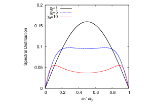
Figure 1: (Color online) The spectral distribution of the created particles $[(2\pi)/(\epsilon_{0}^{2}\,T)]\,dN/d\omega$ as a function of $\omega/\omega_{0}$ for several values of $\gamma_{0}$. Notice the reflexion symmetry around $\omega/\omega_{0}=0.5$: a signature of the fact that particles are created in pairs. The full line corresponds to $\gamma_{0}=1$; the dashed line to $\gamma_{0}=5$ and $20\times[(2\pi)/(\epsilon_{0}^{2}\,T)]\,dN/d\omega$; and the dotted line to $\gamma_{0}=10$ and $100\times[(2\pi)/(\epsilon_{0}^{2}\,T)]\,dN/d\omega$.

A few comments are in order. Firstly, observe (see Fig. 1 and Eq. (20)) that ${dN(\omega)}/{d\omega}$ vanishes for $\omega>\omega_{0}$, which means that no particles are created with frequencies larger than $\omega_{0}$ $-$ the characteristic frequency of the time-dependent BC. We also notice that the spectrum is left invariant under the replacement $\omega\rightarrow\omega_{0}-\omega$. This is a signature of the fact that particles are created in pairs: for each particle created with frequency $\omega$ there is a twin particle created with frequency $\omega_{0}-\omega$. In second place, note that for $\epsilon_{0}\rightarrow 0$, where a Robin BC with a time-independent parameter $\gamma_{0}$ is re-obtained, the spectrum of created particles vanishes, as expected (recall that the mirror which imposes the BC on the field is at rest). Further, for a fixed (finite) value of $\omega_{0}$, the limit $\gamma_{0}\rightarrow\infty$ (Neumann BC imposed on the field at a static mirror) also leads to a vanishing spectrum of created particles. Finally, since we assumed $\epsilon_{0}\ll\gamma_{0}$, the limit $\gamma_{0}\rightarrow 0$ (Dirichlet BC imposed on the field by a static mirror) necessarily leads to a vanishing spectrum as well.

IV Particle creation rate

The total number of created particles is obtained by substituting Eq. (20) in (16), namely,

$$N = \left(\frac{\epsilon^{2}_{0}T}{2\pi}\right)\int_{0}^{\infty}\!\!\frac{\;\omega\,(\omega_{0}-\omega)\,\Theta(\omega_{0}-\omega)}{(1+\gamma_{0}^{2}\omega^{2})\left[1+\gamma_{0}^{2}(\omega_{0}-\omega)^{2}\right]}\,\;d\omega$$ (21)

$$= \left(\frac{\epsilon^{2}_{0}\omega^{3}_{0}T}{2\pi}\right)F(\xi)\;,$$ (23)

where $\xi=\gamma_{0}\omega_{0}$ and the function $F(\xi)$ is given by

$$F(\xi)=\frac{\left(2+\xi^{2}\right)\ln\left(1+\xi^{2}\right)-2\xi\arctan(\xi)}{\xi^{4}\left(4+\xi^{2}\right)}.$$ (24)

As $N$ is proportional to $T$ - as expected for an open cavity - the physical meaningful quantity is the particle creation rate defined as $R=N/T$, that is

$$R=\left(\frac{\epsilon^{2}_{0}\omega^{3}_{0}}{2\pi}\right)F(\xi)\;.$$ (25)

In the limits $\gamma_{0}\omega_{0}\ll 1$ and $\gamma_{0}\omega_{0}\gg 1$, the particle creation rate are approximately given by

$$R\approx\left(\frac{\epsilon^{2}_{0}\omega^{3}_{0}}{12\pi}\right)\;\;\;\;\mbox{for $\;\;\gamma_{0}\omega_{0}\ll 1$}$$ (26)

$$R\approx\left(\frac{\epsilon^{2}_{0}\omega^{3}_{0}}{2\pi}\right)\frac{2\ln(\xi)}{\xi^{4}}\;\;\;\;\mbox{for $\;\;\gamma_{0}\omega_{0}\gg 1$}.$$ (27)

For the sake of comparison with Eq. (25), we recall the total particle creation rates for moving mirrors with Dirichlet Jaekel-PRL-1996 (or equivalently for Neumann BC as proved in equivalencia-DN )

$$R_{\mbox{\footnotesize{D/N}}}=\frac{\delta q^{2}_{0}\omega^{3}_{0}}{12\pi},$$ (28)

and for time-independent Robin BC Mintz-JPA-2006-2

$$R_{\mbox{\footnotesize{ti-R}}}=\left(\frac{\delta q^{2}_{0}\omega_{0}^{3}}{2\pi}\right)G(\gamma_{0}\omega_{0}),$$ (29)

where

$$G(\xi)=\frac{\xi\left[4\xi+\xi^{3}+12\arctan(\xi)\right]-6\left(2+\xi^{2}\right)\ln\left(1+\xi^{2}\right)}{6\xi^{2}\left(4+\xi^{2}\right)}.$$

The formulas above were obtained assuming a non-relativistically small amplitude oscillatory law of motion for the mirror. For both cases $\delta q_{0}$ is the amplitude and $\omega_{0}$ is the frequency of oscillation. We remark that for $\gamma_{0}\omega_{0}\ll 1$ the particle creation rate in our model is exactly the same as for of a moving mirror Jaekel-PRL-1996 with Dirichlet BC where $\epsilon_{0}$ plays the role of the amplitude of oscillation of the motion. This reinforces the possibility of simulating moving boundaries through a static mirror with time-dependent Robin BC. The three particle creation rates are compared in Fig. 2.

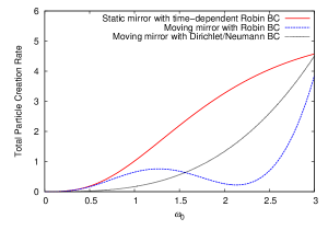
Figure 2: (Color online) Comparison between the total particle creation rates given by Eqs. (25), (28) and (29). The full line corresponds to scaled creation rate $10\times\left[\left(2\pi\gamma_{0}^{3}\right)/\left(\epsilon_{0}^{2}\right)\right]\,R$. The dashed line corresponds to $10\times\left[\left(2\pi\gamma_{0}^{3}\right)/\left(\delta q_{0}^{2}\right)\right]\,R_{\mbox{\footnotesize{ti-R}}}$. Finally, the dotted line corresponds to $\left[\left(2\pi\right)/\left(\delta q_{0}^{2}\right)\right]\,R_{\mbox{\footnotesize{D/N}}}$. In both curves involving Robin BC we considered $\gamma_{0}=1$.

It is worth noting that the particle creation rate shown in Fig. 3 starts growing with $\omega_{0}$ until it achieves a maximum value for a given value of $\omega_{0}$ and then it approaches monotonically to zero as $\omega_{0}$ goes to infinity. This behaviour should be compared with that obtained for a moving mirror which imposes on the field a Robin BC with a time-independent parameter, where the particle creation rate after passing through one maximum and one minimum grows indefinitely as $\omega_{0}$ goes to infinity (see Ref. Mintz-JPA-2006-2 ). Naively, we could expect similar behaviors for these two problems, after all, a time-dependent Robin parameter should simulate, in principle, a moving mirror so that a high frequency oscillating $\gamma(t)$ should mean a high frequency oscillating mirror. However, the interpretation of the Robin parameter $\gamma$ as an estimative of the penetration depth of the material boundary is rigorously proved only for static mirrors. Even in this case, this identification is valid only for the field modes whose frequencies are much smaller than the plasma frequency (but this condition is easily achieved since the plasma frequency is much higher than the mechanical frequencies we want to simulate). It is plausible that such an interpretation remains valid for slowly time-varying $\gamma(t)$, but not for high frequency oscillating $\gamma(t)$. In fact, our results show that this interpretation for $\gamma(t)$ fails for high values of $\omega_{0}$.

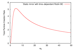
Figure 3: (Color online) Behavior of Eq. (25) for a larger range of $\omega_{0}$, assuming $\gamma_{0}=1$. The creation rate approaches smoothly to zero as $\omega_{0}\rightarrow\infty$. This does not happen for the other cases showed in the Fig. 2: for moving mirrors the particle creation rate increases unlimitedly for larger values of $\omega_{0}$.

V Conclusions and final remarks

Exploring the peculiar properties of Robin BC, particularly, the interpretation of the Robin parameter, we presented a simple and yet instructive theoretical model where a single static mirror with time-dependent properties described by a time-dependent Robin parameter simulates a moving boundary. We used this model to study analytically the dynamical Casimir effect of a system that may of some value for further understanding of a ongoing experiment based on a one-dimensional transmission line terminated by a SQUID. In this setup a time-dependent magnetic flux through the SQUID gives rise to particle creation phenomenon. Employing a perturbative approach, we showed that particles can be created due to the time-dependence of the Robin parameter $\gamma$. We obtained explicitly the spectrum of the created particles as well as the total particle creation rate for a particular choice of $\gamma(t)$ which has a practical interest concerning the experiment just described. Our model can also be used as a theoretical model to investigate other experimental setups suggested for measuring the dynamical Casimir effect, as for example, the promising experimental proposal of the Padua group Experimento-MIR . All we have to do is to choose appropriately the time-dependence of $\gamma(t)$ to simulate correctly the physical situation under consideration.

We emphasize that the particle creation phenomena due to a time-dependent Robin BC imposed on the field at a static mirror has similarities and differences with the case where a time-independent Robin BC is imposed on the field at a moving mirror, as discussed by Mintz et al Mintz-JPA-2006-2 . The main difference being the respective behaviors of the total particle creation rate for high values of $\omega_{0}$ (in the former case, where $\omega_{0}$ means the mechanical frequency of the moving mirror, this rate grows indefinitely as $\omega_{0}\rightarrow\infty$, while in the latter case, where $\omega_{0}$ gives a measure of how quick the time-dependent Robin parameter $\gamma(t)$ varies, this rate goes to zero, as $\omega_{0}\rightarrow\infty$). In the appropriate limits of the usual time-independent Dirichlet ($\gamma_{0}\rightarrow 0$), Neumann ($\gamma_{0}\rightarrow\infty$) and Robin ($\delta\gamma(t)=0$) BCs no particles are created, as expected. The generalization of the present work for 3+1 dimensions and cavities are also expected to have induced photon creation. These issues are under investigation and will be discussed elsewhere.

References

- (1) E. Yablonovitch, Phys. Rev. Lett. 62, 1742 (1989).
- (2) J. Schwinger, Proc. Nat. Acad. Sci. USA 89, 4091 (1992).
- (3) G. T. Moore, J. Math. Phys. 11, 2679 (1970).
- (4) B. S. DeWitt, Phys. Rep. 19, 295 (1975).
- (5) S. A. Fulling and P. C. W. Davies, Proc. R. Soc. London A 348, 393 (1976); P. C. W. Davies and S. A. Fulling, Proc. R. Soc. London A 356, 237 (1977); P. C. W. Davies and S. A. Fulling, Proc. R. Soc. London A 354, 59 (1977); P. Candelas and D. J. Raine, J. Math. Phys. 17, 2101 (1976); P. Candelas and D. Deutsch, Proc. R. Soc. London A 354, 79 (1977).
- (6) V. V. Dodonov, Adv. Chem. Phys. 119, 309 (2001) [arXiv:quant-ph/0106081v1]. V. V. Dodonov, J. Phys.: Conf. Ser. 161, 012027 (2009); D. A. R. Dalvit, P. A. Maia Neto and F.D. Mazzitelli, arXiv:1006.4790v2 (2010); V. V. Dodonov, Phys. Scr. 82, 038105 (2010).
- (7) L. H. Ford and A. Vilenkin, Phys. Rev. D 25, 2569 (1982); P. A. Maia Neto, J. Phys. A 27, 2167 (1994); P. A. Maia Neto and L. A. S. Machado, Phys. Rev. A 54, 3420 (1996); P. A. Maia Neto and L. A. S. Machado, Braz. J. Phys. 25, 324 (1996).
- (8) A. Lambrecht, M.-T. Jaekel and S. Reynaud, Phys. Rev. Lett. 77, 615 (1996).
- (9) B. Mintz, C. Farina, P. A. Maia Neto and R. B. Rodrigues, J. Phys. A: Math. Gen. 39, 6559 (2006).
- (10) B. Mintz, C. Farina, P. A. Maia Neto and R. B. Rodrigues, J. Phys. A: Math. Gen. 39, 11325 (2006).
- (11) C. K. Law, Phys. Rev. Lett. 73, 1931 (1994); Y. Wu, K. W. Chan, M. C. Chu and P. T. Leung, Phys. Rev. A 59, 1662 (1999); P. Wegrzyn, J. Phys. B 40, 2621 (2007); V. V. Dodonov, A. B. Klimov and D. E. Nikonov, J. Math. Phys. 34, 2742 (1993); D. A. R. Dalvit and F. D. Mazzitelli, Phys. Rev. A 57, 2113 (1998); C. K. Cole and W. C. Schieve, Phys. Rev. A 52, 4405 (1995); C. K. Cole and W. C. Schieve, Phys. Rev. A 64, 023813 (2001); M. Razavy and J. Terning, Phys. Rev. D 31, 307 (1985); G. Calucci, J. Phys. A 25, 3873 (1992); C. K. Law, Phys. Rev. A 49, 433 (1994); V. V. Dodonov and A. B. Klimov, Phys. Rev. A 53, 2664 (1996); D. F. Mundarain and P.A. Maia Neto, Phys. Rev. A 57, 1379 (1998); D. T. Alves, C. Farina and E. R. Granhen, Phys. Rev. A 73, 063818 (2006); J. Sarabadani and M. F. Miri, Phys. Rev. A 75, 055802 (2007).
- (12) M.-T. Jaekel and S. Reynaud, J. Phys. I (France) 3, 339 (1993); M.-T. Jaekel and S. Reynaud, Phys. Lett. A 172, 319 (1993); L. A. S. Machado, P. A. Maia Neto and C. Farina, Phys. Rev. D 66, 105016 (2002).
- (13) D. T. Alves, C. Farina and P. A. Maia Neto, J. Phys. A 36, 11333 (2003); D. T. Alves, E. R. Granhen and M. G. Lima, Phys. Rev. D 77, 125001 (2008).
- (14) V. V. Dodonov, J. Phys. A: Math. Gen. 31, 9835 (1998); G. Plunien, R. Schützhold and G. Soff, Phys. Rev. Lett. 84, 1882 (2000); J. Hui, S. Qing-Yun and W. Jian-Sheng, Phys. Lett. A 268, 174 (2000); R. Schützhold, G. Plunien and G. Soff, Phys. Rev. A 65, 043820 (2002); G. Schaller, R. Schützhold, G. Plunien and G. Soff, Phys. Rev. A 66, 023812 (2002); D. T. Alves, E. R. Granhen, H. O. Silva and M. G. Lima, Phys. Rev. D 81, 025016 (2010).
- (15) C. M. Wilson et al, arXiv:1105.4714v1 (2011).
- (16) E. Yablonovitch, J. P. Heritage, D. E. Aspnes and Y. Yafet, Phys. Rev. Lett. 63, 976 (1989); Y. E. Lozovik, V. G. Tsvetus and E. A. Vinogradov, JETP Lett. 61, 723 (1995); Y. E. Lozovik, V. G. Tsvetus and E. A. Vinogradov, Phys. Scr. 52, 184 (1995); T. Okushima and A. Shimizu, Japan J. Appl. Phys. 34, 4508 (1995); M. Uhlmann, G. Plunien, R. Schützhold and G. Soff, Phys. Rev. Lett. 93, 193601 (2004).
- (17) W. Naylor, S. Matsuki, T. Nishimura and Y. Kido, Phys. Rev. A 80, 043835 (2009).
- (18) M. Crocce, D. A. R. Dalvit, F. C. Lombardo and F. D. Mazzitelli, Phys. Rev. A 70, 033811 (2004).
- (19) C. Braggio et al, Europhys. Lett. 70, 754 (2005); A. Agnesi et al, J. Phys. A: Math. Gen. 41, 164024 (2008); A. Agnesi et al, J. Phys.: Conf. Ser. 161, 012028 (2009).
- (20) J. R. Johansson, G. Johansson, C. M. Wilson and F. Nori, Phys. Rev. Lett. 103, 147003 (2009); J. R. Johansson, G. Johansson, C. M. Wilson and F. Nori, Phys. Rev. A 82, 052509 (2010).
- (21) P. D. Nation, J. R. Johansson, M. P. Blencowe and F. Nori, arXiv:1103.0835v1 (2011).
- (22) C. M. Wilson et al, Phys. Rev. Lett. 105, 233907 (2010).
- (23) K. Gustafson, Introduction to Partial Differential Equations and Hilbert Space Methods (Dover Publications, New York, 1999); G. Chen, J. Zhou, Vibration and Damping in Distributed Systems vol. 1 (CRC Press, Florida, 1999).
- (24) T. E. Clark, R. Menikoff and D. H. Sharp, Phys. Rev. D 22, 3012 (1980); M. Carreau, E. Farhi and S. Gutmann, Phys. Rev. D 42, 1194 (1990); V. S. Araujo, F. A. B. Countinho and J. Fernando Perez, Am. J. Phys. 72, 203 (2004); V. S. Araujo, F. A. B. Coutinho and F. M. Toyama, Braz. J. Phys. 38, 178 (2008); B. Belchev and M. A. Walton, J. Phys. A: Math. Gen. 43, 085301 (2010).
- (25) H. B. G. Casimir, Proc. K. Nede. Akad. Wet. B51, 793 (1948).
- (26) A. Romeo and A. A. Saharian, J. Phys. A: Math. Gen. 35, 1297 (2002).
- (27) T. H. Boyer, Phys. Rev. A 9, 2078 (1974).
- (28) Z. H. Liu and S. A. Fulling, New J. Phys. 8, 234 (2006); E. Elizalde, S. D. Odintsov and A. A. Saharian, Phys. Rev. D 79 065023 (2009); L. P. Teo, JHEP 11, 095 (2009); M. Asorey, D. García Álvares and J. M. Muñoz-Castañeda, J. Phys. A: Math. Gen. 39, 6127 (2006).
- (29) M. Asorey and J. M. Muñoz-Castañeda, J. Phys. A: Math. Theor. 41, 164043 (2008); M. Asorey and J. M. Muñoz-Castañeda, J. Phys. A: Math. Theor. 41, 304004 (2008).
- (30) V. M. Mostepanenko and N. N. Trunov, Sov. J. Nucl. Phys. 45, 818 (1985).
- (31) See the first reference of Single-mirror .