A Constrained $\ell_{1}$ Minimization Approach to Sparse Precision Matrix Estimation

Abstract

A constrained $\ell_{1}$ minimization method is proposed for estimating a sparse inverse covariance matrix based on a sample of $n$ iid $p$-variate random variables. The resulting estimator is shown to enjoy a number of desirable properties. In particular, it is shown that the rate of convergence between the estimator and the true $s$-sparse precision matrix under the spectral norm is $s\sqrt{\log p/n}$ when the population distribution has either exponential-type tails or polynomial-type tails. Convergence rates under the elementwise $\ell_{\infty}$ norm and Frobenius norm are also presented. In addition, graphical model selection is considered. The procedure is easily implementable by linear programming. Numerical performance of the estimator is investigated using both simulated and real data. In particular, the procedure is applied to analyze a breast cancer dataset. The procedure performs favorably in comparison to existing methods.

Keywords: constrained $\ell_{1}$ minimization, covariance matrix, Frobenius norm, Gaussian graphical model, rate of convergence, precision matrix, spectral norm.

1 Introduction

Estimation of covariance matrix and its inverse is an important problem in many areas of statistical analysis. Among many interesting examples are principal component analysis, linear/quadratic discriminant analysis, and graphical models. Stable and accurate covariance estimation is becoming increasingly more important in the high dimensional setting where the dimension $p$ can be much larger than the sample size $n$. In this setting classical methods and results based on fixed $p$ and large $n$ are no longer applicable. An additional challenge in the high dimensional setting is the computational costs. It is important that estimation procedures are computationally effective so that they can be used in high dimensional applications.

Let $\textbf{X}=(X_{1},\dotsc,X_{p})$ be a $p$-variate random vector with covariance matrix $\boldsymbol{\Sigma}_{0}$ and precision matrix $\boldsymbol{\Omega}_{0}:=\boldsymbol{\Sigma}_{0}^{-1}$. Given an independent and identically distributed random sample $\{\textbf{X}_{1},\dotsc,\textbf{X}_{n}\}$ from the distribution of X, the most natural estimator of $\boldsymbol{\Sigma}_{0}$ is perhaps

$$\boldsymbol{\Sigma}_{n}=\frac{1}{n}\sum_{k=1}^{n}(\textbf{X}_{k}-\bar{\textbf{X}})(\textbf{X}_{k}-\bar{\textbf{X}})^{T},$$

where $\bar{\textbf{X}}=n^{-1}\sum_{k=1}^{n}\textbf{X}_{k}$. However, $\boldsymbol{\Sigma}_{n}$ is singular if $p>n$, and thus is unstable for estimating $\boldsymbol{\Sigma}_{0}$, not to mention that one cannot use its inverse to estimate the precision matrix $\boldsymbol{\Omega}_{0}$. In order to estimate the covariance matrix $\boldsymbol{\Sigma}_{0}$ consistently, special structures are usually imposed and various estimators have been introduced under these assumptions. When the variables exhibit a certain ordering structure, which is often the case for time series data, Bickel and Levina (2008a) proved that banding the sample covariance matrix leads to a consistent estimator. Cai, Zhang and Zhou (2010) established the minimax rate of convergence and introduced a rate-optimal tapering estimator. El Karoui (2008) and Bickel and Levina (2008b) proposed thresholding of the sample covariance matrix for estimating a class of sparse covariance matrices and obtained rates of convergence for the thresholding estimators.

Estimation of the precision matrix $\boldsymbol{\Omega}_{0}$ is more involved due to the lack of a natural pivotal estimator like $\boldsymbol{\Sigma}_{n}$. Assuming certain ordering structures, methods based on banding the Cholesky factor of the inverse have been proposed and studied. See, e.g., Wu and Pourahmadi (2003), Huang et al. (2006), Bickel and Levina (2008b). Penalized likelihood methods have also been introduced for estimating sparse precision matrices. In particular, the $\ell_{1}$ penalized normal likelihood estimator and its variants, which shall be called $\ell_{1}$-MLE type estimators, were considered in several papers; see, for example, Yuan and Lin (2007), Friedman et al. (2008), d’Aspremont et al.  (2008), and Rothman et al. (2008). Convergence rate under the Frobenius norm loss was given in Rothman et al. (2008). Yuan (2009) derived the rates of convergence for subgaussian distributions. Under more restrictive conditions such as mutual incoherence or irrepresentable conditions, Ravikumar et al. (2008) obtained the rates of convergence in the elementwise $\ell_{\infty}$ norm and spectral norm. Nonconvex penalties, usually computationally more demanding, have also been considered under the same normal likelihood model. For example, Lam and Fan (2009) and Fan et al. (2009) considered penalizing the normal likelihood with the nonconvex SCAD penalty. The main goal is to ameliorate the bias problem due to $\ell_{1}$ penalization.

A closely related problem is the recovery of the support of the precision matrix, which is strongly connected to the selection of graphical models. To be more specific, let $G=(V,E)$ be a graph representing conditional independence relations between components of X. The vertex set $V$ has $p$ components $X_{1},\dotsc,X_{p}$ and the edge set $E$ consists of ordered pairs $(i,j)$, where $(i,j)\in E$ if there is an edge between $X_{i}$ and $X_{j}$. The edge between $X_{i}$ and $X_{j}$ is excluded from $E$ if and only if $X_{i}$ and $X_{j}$ are independent given $(X_{k},k\neq i,j)$. If $\textbf{X}\sim N(\boldsymbol{\mu}_{0},\boldsymbol{\Sigma}_{0})$, then the conditional independence between $X_{i}$ and $X_{j}$ given other variables is equivalent to $\omega^{0}_{ij}=0$, where we set $\boldsymbol{\Omega}_{0}=(\omega^{0}_{ij})$. Hence, for Gaussian distributions, recovering the structure of the graph $G$ is equivalent to the estimation of the support of the precision matrix (Lauritzen (1996)). A recent paper by Liu et al. (2009) showed that for a class of non-Gaussian distribution called nonparanormal distribution, the problem of estimating the graph can also be reduced to the estimation of the precision matrix. In an important paper, Meinshausen and Bühlmann (2006) demonstrated convincingly a neighborhood selection approach to recover the support of $\boldsymbol{\Omega}_{0}$ in a row by row fashion. Yuan (2009) replaced the lasso selection by a Dantzig type modification, where first the ratios between the off-diagonal elements $\omega_{ij}$ and the corresponding diagonal element $\omega_{ii}$ were estimated for each row $i$ and then the diagonal entries $\omega_{ii}$ were obtained given the estimated ratios. Convergence rates under the matrix $\ell_{1}$ norm and spectral norm losses were established.

In the present paper, we study estimation of the precision matrix $\boldsymbol{\Omega}_{0}$ for both sparse and non-sparse matrices, without restricting to a specific sparsity pattern. In addition, graphical model selection is also considered. A new method of constrained $\ell_{1}$-minimization for inverse matrix estimation (CLIME) is introduced. Rates of convergence in spectral norm as well as elementwise $\ell_{\infty}$ norm and Frobenius norm are established under weaker assumptions, and are shown to be faster than those given for the $\ell_{1}$-MLE estimators when the population distribution has polynomial-type tails. A matrix is called $s$-sparse if there are at most $s$ non-zero elements on each row. It is shown that when $\boldsymbol{\Omega}_{0}$ is $s$-sparse and X has either exponential-type or polynomial-type tails, the error between our estimator $\hat{\boldsymbol{\Omega}}$ and $\boldsymbol{\Omega}_{0}$ satisfies $\|\hat{\boldsymbol{\Omega}}-\boldsymbol{\Omega}_{0}\|_{2}=O_{\textsf{P}}(s\sqrt{\log p/n})$ and $|\hat{\boldsymbol{\Omega}}-\boldsymbol{\Omega}_{0}|_{\infty}=O_{\textsf{P}}(\sqrt{\log p/n})$, where $\|\cdot\|_{2}$ and $|\cdot|_{\infty}$ are the spectral norm and elementwise $l_{\infty}$ norm respectively. Properties of the CLIME estimator for estimating banded precision matrices are also discussed. The CLIME method can also be adopted for the selection of graphical models, with an additional thresholding step. The elementwise $\ell_{\infty}$ norm result is instrumental for graphical model selection.

In addition to its desirable theoretical properties, the CLIME estimator is computationally very attractive for high dimensional data. It can be obtained one column at a time by solving a linear program, and the resulting matrix estimator is formed by combining the vector solutions (after a simple symmetrization). No outer iterations are needed and the algorithm is easily scalable. An R package of our method has been developed and is publicly available on the web. Numerical performance of the estimator is investigated using both simulated and real data. In particular, the procedure is applied to analyze a breast cancer dataset. Results show that the procedure performs favorably in comparison to existing methods.

The rest of the paper is organized as follows. In Section 2, after basic notations and definitions are introduced, we present the CLIME estimator. Theoretical properties including the rates of convergence are established in Section 3. Graphical model selection is discussed in Section 4. Numerical performance of the CLIME estimator is considered in Section 5 through simulation studies and a real data analysis. Further discussions on the connections and differences of our results with other related work are given in Section 6. The proofs of the main results are given in Section 7.

2 Estimation via Constrained $\ell_{1}$ Minimization

In compressed sensing and high dimensional linear regression literature, it is now well understood that constrained $\ell_{1}$ minimization provides an effective way for reconstructing a sparse signal. See, for example, Donoho et al. (2006) and Candès and Tao (2007). A particularly simple and elementary analysis of constrained $\ell_{1}$ minimization methods is given in Cai, Wang and Xu (2010).

In this section, we introduce a method of constrained $\ell_{1}$ minimization for inverse covariance matrix estimation. We begin with basic notations and definitions. Throughout, for a vector $\textbf{a}=(a_{1},\dotsc,a_{p})^{T}\in I\!\!R^{p}$, define $|\textbf{a}|_{1}=\sum_{j=1}^{p}|a_{j}|$ and $|\textbf{a}|_{2}=\sqrt{\sum_{j=1}^{p}a^{2}_{j}}$. For a matrix $\boldsymbol{A}=(a_{ij})\in I\!\!R^{p\times q}$, we define the elementwise $l_{\infty}$ norm $|\boldsymbol{A}|_{\infty}=\max_{1\leq i\leq p,1\leq j\leq q}|a_{ij}|$, the spectral norm $\|\boldsymbol{A}\|_{2}=\sup_{|\textbf{x}|_{2}\leq 1}|\boldsymbol{A}\textbf{x}|_{2}$, the matrix $\ell_{1}$ norm $\|\boldsymbol{A}\|_{L_{1}}=\max_{1\leq j\leq q}\sum_{i=1}^{p}|a_{ij}|$, the Frobenius norm $\|\boldsymbol{A}\|_{F}=\sqrt{\sum_{i,j}a^{2}_{ij}}$, and the elementwise $\ell_{1}$ norm $\|\boldsymbol{A}\|_{1}=\sum_{i=1}^{p}\sum_{j=1}^{q}|a_{i,j}|$. $\boldsymbol{I}$ denotes a $p\times p$ identity matrix. For any two index sets $T$ and $T^{{}^{\prime}}$ and matrix $\boldsymbol{A}$, we use $\boldsymbol{A}_{TT^{{}^{\prime}}}$ to denote the $|T|\times|T^{{}^{\prime}}|$ matrix with rows and columns of $\boldsymbol{A}$ indexed by $T$ and $T^{{}^{\prime}}$ respectively. The notation $\boldsymbol{A}\succ 0$ means that $\boldsymbol{A}$ is positive definite.

We now define our CLIME estimator. Let $\{\hat{\boldsymbol{\Omega}}_{1}\}$ be the solution set of the following optimization problem:

$$\min\|\boldsymbol{\Omega}\|_{1}~{}~{}\mbox{subject to:}~{}~{}|\boldsymbol{\Sigma}_{n}\boldsymbol{\Omega}-\boldsymbol{I}|_{\infty}\leq\lambda_{n},~{}~{}\boldsymbol{\Omega}\in I\!\!R^{p\times p},$$ (1)

where $\lambda_{n}$ is a tuning parameter. In (1), we do not impose the symmetry condition on $\boldsymbol{\Omega}$ and as a result the solution is not symmetric in general. The final CLIME estimator of $\boldsymbol{\Omega}_{0}$ is obtained by symmetrizing $\hat{\boldsymbol{\Omega}}_{1}$ as follows. Write $\hat{\boldsymbol{\Omega}}_{1}=(\hat{\omega}^{1}_{ij})=(\hat{\boldsymbol{\omega}}^{1}_{1},\dotsc,\hat{\boldsymbol{\omega}}^{1}_{p})$. The CLIME estimator $\hat{\boldsymbol{\Omega}}$ of $\boldsymbol{\Omega}_{0}$ is defined as

$$\hat{\boldsymbol{\Omega}}=(\hat{\omega}_{ij}),~{}~{}\mbox{where~{}~{}}\hat{\omega}_{ij}=\hat{\omega}_{ji}=\hat{\omega}^{1}_{ij}I\{|\hat{\omega}^{1}_{ij}|\leq|\hat{\omega}^{1}_{ji}|\}+\hat{\omega}^{1}_{ji}I\{|\hat{\omega}^{1}_{ij}|>|\hat{\omega}^{1}_{ji}|\}.$$ (2)

In other words, between $\hat{\omega}^{1}_{ij}$ and $\hat{\omega}^{1}_{ji}$, we take the one with smaller magnitude. It is clear that $\hat{\boldsymbol{\Omega}}$ is a symmetric matrix. Moreover, Theorem 1 shows that it is positive definite with high probability.

The convex program (1) can be further decomposed into $p$ vector minimization problems. Let $\boldsymbol{e}_{i}$ be a standard unit vector in $I\!\!R^{p}$ with $1$ in the $i$-th coordinate and $0$ in all other coordinates. For $1\leq i\leq p$, let $\hat{\boldsymbol{\bf\beta}}_{i}$ be the solution of the following convex optimization problem

$$\min|\boldsymbol{\beta}|_{1}~{}~{}\mbox{subject to}~{}~{}|\boldsymbol{\Sigma}_{n}\boldsymbol{\beta}-\boldsymbol{e}_{i}|_{\infty}\leq\lambda_{n},$$ (3)

where $\boldsymbol{\beta}$ is a vector in $I\!\!R^{p}$. The following lemma shows that solving the optimization problem (1) is equivalent to solving the $p$ optimization problems (3). That is, $\{\hat{\boldsymbol{\Omega}}_{1}\}=\{\hat{\textbf{B}}\}:=\{(\hat{\boldsymbol{\beta}}_{1},\dotsc,\hat{\boldsymbol{\beta}}_{p})\}$. This simple observation is useful both for implementation and technical analysis.

Lemma 1

Let $\{\hat{\boldsymbol{\Omega}}_{1}\}$ be the solution set of (1) and let $\{\hat{\textbf{B}}\}:=\{(\hat{\boldsymbol{\beta}}_{1},\dotsc,\hat{\boldsymbol{\beta}}_{p})\}$ where $\hat{\boldsymbol{\beta}}_{i}$ are solutions to (3) for $i=1,...,p$. Then $\{\hat{\boldsymbol{\Omega}}_{1}\}=\{\hat{\textbf{B}}\}$.

To illustrate the motivation of (1), let us recall the method based on $\ell_{1}$ regularized log-determinant program (cf. d’Aspremont et al. (2008), Friedman et al. (2008), Banerjee et al.  (2008)) as follows, which shall be called Glasso after the algorithm that efficiently computes the solution,

$$\hat{\boldsymbol{\Omega}}_{\rm Glasso}:=\mathop{\rm arg\min}_{\Theta\succ 0}\{\langle\boldsymbol{\Omega},\boldsymbol{\Sigma}_{n}\rangle-\log\det(\boldsymbol{\Omega})+\lambda_{n}\|\boldsymbol{\Omega}\|_{1}\}.$$ (4)

The solution $\hat{\boldsymbol{\Omega}}_{\rm Glasso}$ satisfies

$$\hat{\boldsymbol{\Omega}}_{\rm Glasso}^{-1}-\boldsymbol{\Sigma}_{n}=\lambda_{n}\hat{\boldsymbol{Z}},$$

where $\hat{\boldsymbol{Z}}$ is an element of the subdifferential $\partial\|\hat{\boldsymbol{\Omega}}_{\rm Glasso}\|_{1}$. This leads us to consider the optimization problem:

$$\min\|\boldsymbol{\Omega}\|_{1}~{}~{}\mbox{subject to:}~{}~{}|\boldsymbol{\Omega}^{-1}-\boldsymbol{\Sigma}_{n}|_{\infty}\leq\lambda_{n},~{}~{}\boldsymbol{\Omega}\in I\!\!R^{p\times p}.$$ (5)

However, the feasible set in (5) is very complicated. By multiplying the constraint with $\boldsymbol{\Omega}$, such a relaxation of (5) leads to the convex optimization problem (1), which can be easily solved. Figure 1 illustrates the solution for recovering a $2$ by $2$ precision matrix $[\begin{smallmatrix}x&z\\ z&y\end{smallmatrix}]$, and we only consider the plane $x(=y)$ vs $z$ for simplicity. The point where the feasible polygon meets the dashed diamond is the CLIME solution $\hat{\boldsymbol{\Omega}}$. Note that the log-likelihood function as in Glasso is a smooth curve as compared to the polygon constraint in CLIME.

Figure 1: Plot of the elementwise $\ell_{\infty}$ constrained feasible set (shaded polygon) and the elementwise $\ell_{1}$ norm objective (dashed diamond near the origin) from CLIME. The log-likelihood function as in Glasso is shown by the dotted line.

3 Rates of Convergence

In this section we investigate the theoretical properties of the CLIME estimator and establish the rates of convergence under different norms. Write $\boldsymbol{\Sigma}_{n}=(\hat{\sigma}_{ij})=(\hat{\sigma}_{1},\dotsc,\hat{\sigma}_{p})$, $\boldsymbol{\Sigma}_{0}=(\sigma^{0}_{ij})$ and $\textsf{E}\textbf{X}=(\mu_{1},\dotsc,\mu_{p})$. It is conventional to divide the technical analysis into two cases according to the moment conditions on X.

(C1). (Exponential-type tails) Suppose that there exists some $0<\eta<1/4$ such that $\log p/n\leq\eta$ and

$$\textsf{E}e^{t(X_{i}-\mu_{i})^{2}}\leq K<\infty~{}~{}~{}\mbox{for all $|t|\leq\eta$, for all $i$},$$

where $K$ is a bounded constant.

(C2). (Polynomial-type tails) Suppose that for some $\gamma,c_{1}>0$, $p\leq c_{1}n^{\gamma}$, and for some $\delta>0$

$$\textsf{E}|X_{i}-\mu_{i}|^{4\gamma+4+\delta}\leq K~{}~{}~{}\mbox{for all $i$.}$$

For $\ell_{1}$-MLE type estimators, it is typical that the convergence rates in the case of polynomial-type tails are much slower than those in the case of exponential-type tails. See, e.g., Ravikumar et al. (2008). We shall show that our CLIME estimator attains the same rates of convergence under either of the two moment conditions, and significantly outperforms $\ell_{1}$-MLE type estimators in the case of polynomial-type tails.

3.1 Rates of convergence under spectral norm

We begin by considering the uniformity class of matrices:

$$\mathcal{U}:=\mathcal{U}(q,s_{0}(p))=\Big{\{}\boldsymbol{\Omega}:\boldsymbol{\Omega}\succ 0,~{}\|\boldsymbol{\Omega}\|_{L_{1}}\leq M,~{}\max_{1\leq i\leq p}\sum_{j=1}^{p}|\omega_{ij}|^{q}\leq s_{0}(p)\Big{\}}$$

for $0\leq q<1$, where $\boldsymbol{\Omega}=:(\omega_{ij})=(\boldsymbol{\omega}_{1},\dotsc,\boldsymbol{\omega}_{p})$. Similar parameter spaces have been used in Bickel and Levina (2008b) for estimating the covariance matrix $\boldsymbol{\Sigma}_{0}$ . Note that in the special case of $q=0$, $\mathcal{U}(0,s_{0}(p))$ is a class of $s_{0}(p)$-sparse matrices. Let

$$\theta=\max_{ij}\textsf{E}\Big{[}(X_{i}-\mu_{i})(X_{j}-\mu_{j})-\sigma^{0}_{ij}\Big{]}^{2}=:\max_{ij}\theta_{ij}.$$

The quantity $\theta_{ij}$ is related to the variance of $\hat{\sigma}_{ij}$, and the maximum value $\theta$ captures the overall variability of $\boldsymbol{\Sigma}_{n}$. It is easy to see that under either (C1) or (C2) $\theta$ is a bounded constant depending only on $\gamma,\delta,K$.

The following theorem gives the rates of convergence for the CLIME estimator $\hat{\boldsymbol{\Omega}}$ under the spectral norm loss.

Theorem 1

Suppose that $\boldsymbol{\Omega}_{0}\in\mathcal{U}(q,s_{0}(p))$.

(i). Assume (C1) holds. Let $\lambda_{n}=C_{0}M\sqrt{\log p/n}$, where $C_{0}=2\eta^{-2}(2+\tau+\eta^{-1}e^{2}K^{2})^{2}$ and $\tau>0$. Then

$$\|\hat{\boldsymbol{\Omega}}-\boldsymbol{\Omega}_{0}\|_{2}\leq C_{1}M^{2-2q}s_{0}(p)\Big{(}\frac{\log p}{n}\Big{)}^{(1-q)/2},$$ (6)

with probability greater than $1-4p^{-\tau}$, where $C_{1}\leq 2(1+2^{1-q}+3^{1-q})4^{1-q}C_{0}^{1-q}$.

(ii). Assume (C2) holds. Let $\lambda_{n}=C_{2}M\sqrt{\log p/n}$, where $C_{2}=\sqrt{(5+\tau)(\theta+1)}$. Then

$$\|\hat{\boldsymbol{\Omega}}-\boldsymbol{\Omega}_{0}\|_{2}\leq C_{3}M^{2-2q}s_{0}(p)\Big{(}\frac{\log p}{n}\Big{)}^{(1-q)/2},$$ (7)

with probability greater than $1-O\Big{(}n^{-\delta/8}+p^{-\tau/2}\Big{)}$, where $C_{3}\leq 2(1+2^{1-q}+3^{1-q})4^{1-q}C^{1-q}_{2}$.

When $M$ does not depend on $n,p$, the rates in Theorem 1 are the same as those for estimating $\boldsymbol{\Sigma}_{0}$ in Bickel and Levina (2008b). In the polynomial-type tails case and when $q=0$, the rate in (7) is significantly better than the rate $O\Big{(}s_{0}(p)\sqrt{\frac{p^{1/(\gamma+1+\delta/4)}}{n}}\Big{)}$ for the $\ell_{1}$-MLE estimator obtained in Ravikumar et al. (2008).

It would be of great interest to get the convergence rates for $\sup_{\boldsymbol{\Omega}_{0}\in\mathcal{U}}\textsf{E}\|\hat{\boldsymbol{\Omega}}-\boldsymbol{\Omega}_{0}\|^{2}_{2}$. However, it is even difficult to prove the existence of the expectation of $\|\hat{\boldsymbol{\Omega}}-\boldsymbol{\Omega}_{0}\|^{2}_{2}$ as we are dealing with the inverse matrix. We modify the estimator $\hat{\boldsymbol{\Omega}}$ to ensure the existence of such expectation and the same rates are established. Let $\{\hat{\boldsymbol{\Omega}}_{1\rho}\}$ be the solution set of the following optimization problem:

$$\min\|\boldsymbol{\Omega}\|_{1}~{}~{}\mbox{subj}~{}~{}|\boldsymbol{\Sigma}_{n,\rho}\boldsymbol{\Omega}-\boldsymbol{I}|_{\infty}\leq\lambda_{n},~{}~{}\boldsymbol{\Omega}\in I\!\!R^{p\times p},$$ (8)

where $\boldsymbol{\Sigma}_{n,\rho}=\boldsymbol{\Sigma}_{n}+\rho\boldsymbol{I}$ with $\rho>0$. Write $\hat{\boldsymbol{\Omega}}_{1\rho}=(\hat{\omega}^{1}_{ij\rho})$. Define the symmetrized estimator $\hat{\boldsymbol{\Omega}}_{\rho}$ as in (2) by

$$\hat{\boldsymbol{\Omega}}_{\rho}=(\hat{\omega}_{ij\rho}),~{}~{}\mbox{where~{}~{}}\hat{\omega}_{ij\rho}=\hat{\omega}_{ji\rho}=\hat{\omega}^{1}_{ij\rho}I\{|\hat{\omega}^{1}_{ij\rho}|\leq|\hat{\omega}^{1}_{ji\rho}|\}+\hat{\omega}^{1}_{ji\rho}I\{|\hat{\omega}^{1}_{ij\rho}|>|\hat{\omega}^{1}_{ji\rho}|\}.$$ (9)

Clearly $\boldsymbol{\Sigma}_{n,\rho}^{-1}$ is a feasible point, and thus we have $\|\hat{\boldsymbol{\Omega}}_{1\rho}\|_{L_{1}}\leq\|\boldsymbol{\Sigma}_{n,\rho}^{-1}\|_{L_{1}}\leq\rho^{-1}p$. The expectation $\textsf{E}\|\hat{\boldsymbol{\Omega}}_{\rho}-\boldsymbol{\Omega}_{0}\|^{2}_{2}$ is then well-defined. The other motivation to replace $\boldsymbol{\Sigma}_{n}$ with $\boldsymbol{\Sigma}_{n,\rho}$ comes from our implementation, which computes (1) by the primal dual interior point method. One usually needs to specify a feasible initialization. When $p>n$, it is hard to find an initial value for (1). For (8), we can simply set the initial value to $\boldsymbol{\Sigma}_{n,\rho}^{-1}$.

Theorem 2

Suppose that $\boldsymbol{\Omega}_{0}\in\mathcal{U}(q,s_{0}(p))$ and (C1) holds. Let $\lambda_{n}=C_{0}M\sqrt{\log p/n}$ with $C_{0}$ being defined in Theorem 1 (i) and $\tau$ being sufficiently large. Let $\rho=\sqrt{\log p/n}.$ If $p\geq n^{\xi}$ for some $\xi>0$, then we have

$$\sup_{\boldsymbol{\Omega}_{0}\in\mathcal{U}}\textsf{E}\|\hat{\boldsymbol{\Omega}}_{\rho}-\boldsymbol{\Omega}_{0}\|^{2}_{2}=O\Big{(}M^{4-4q}s^{2}_{0}(p)\Big{(}\frac{\log p}{n}\Big{)}^{1-q}\Big{)}.$$

Remark: It is not necessary to restrict $\rho=\sqrt{\log p/n}$. In fact, from the proof we can see that Theorem 2 still holds for

$$\min(\sqrt{\frac{\log p}{n}},p^{-\alpha})\leq\rho\leq\sqrt{\frac{\log p}{n}}$$ (10)

with any $\alpha>0$.

When the variables of X are ordered, better rates can be obtained. Similar as in Bickel and Levina (2008a), we consider the following class of precision matrices:

$$\mathcal{U}_{o}(\alpha,B) = \Big{\{}\boldsymbol{\Omega}:\boldsymbol{\Omega}\succ 0,~{}~{}\max_{j}\sum_{i}\{|\omega_{ij}|:|i-j|\geq k\}\leq B(k+1)^{-\alpha}~{}\mbox{for all $k\geq 0$}\Big{\}}$$

for $\alpha>0$. Suppose the modified Cholesky factor of $\boldsymbol{\Omega}_{0}$ is $\boldsymbol{\Omega}_{0}=TD^{-1}T$, with the unique lower triangular matrix $T$ and diagonal matrix $D$. To estimate $\boldsymbol{\Omega}_{0}$, Bickel and Levina (2008a) used the banding method and assumed $T\in\mathcal{U}_{o}(\alpha,B)$. It is easy to see that $T\in\mathcal{U}_{o}(\alpha,B)$ implies $\boldsymbol{\Omega}_{0}\in\mathcal{U}_{o}(\alpha,B_{1})$ for some constant $B_{1}$. Rather than assuming $T\in\mathcal{U}_{o}(\alpha,B)$, we use a more general assumption that $\boldsymbol{\Omega}_{0}\in\mathcal{U}_{o}(\alpha,B)$.

Theorem 3

Let $\boldsymbol{\Omega}_{0}\in\mathcal{U}_{o}(\alpha,B)$ and $\lambda_{n}=CB\sqrt{\log p/n}$ with sufficiently large $C$.

(i). If (C1) or (C2) holds, then with probability greater than $1-O\Big{(}n^{-\delta/8}+p^{-\tau/2}\Big{)}$,

$$\|\hat{\boldsymbol{\Omega}}-\boldsymbol{\Omega}_{0}\|_{2}=O\Big{(}B^{2}\Big{(}\frac{\log p}{n}\Big{)}^{\alpha/(2\alpha+2)}\Big{)}.$$ (11)

(ii). Suppose that $p\geq n^{\xi}$ for some $\xi>0$. If (C1) holds and $\rho=\sqrt{\log p/n}$, then

$$\sup_{\boldsymbol{\Omega}_{0}\in\mathcal{U}_{o}(\alpha,B)}\textsf{E}\|\hat{\boldsymbol{\Omega}}_{\rho}-\boldsymbol{\Omega}_{0}\|^{2}_{2}=O\Big{(}B^{4}\Big{(}\frac{\log p}{n}\Big{)}^{\alpha/(\alpha+1)}\Big{)}.$$ (12)

Theorem 3 shows that our estimator has the same rate as that in Bickel and Levina (2008a) by banding the Cholesky factor of the precision matrix for the ordered variables.

3.2 Rates under $l_{\infty}$ norm and Frobenius norm

We have so far focused on the performance of the estimator under the spectral norm loss. Rates of convergence can also be obtained under the elementwise $l_{\infty}$ norm and the Frobenius norm.

Theorem 4

(i). Under the conditions of Theorem 1 (i), we have

$$|\hat{\boldsymbol{\Omega}}-\boldsymbol{\Omega}_{0}|_{\infty}\leq 4C_{0}M^{2}\sqrt{\frac{\log p}{n}},$$

$$\frac{1}{p}\|\hat{\boldsymbol{\Omega}}-\boldsymbol{\Omega}_{0}\|^{2}_{F}\leq 4C_{1}M^{4-2q}s_{0}(p)\Big{(}\frac{\log p}{n}\Big{)}^{1-q/2},$$

with probability greater than $1-4p^{-\tau}$.

(ii). Under the conditions of Theorem 1 (ii), we have

$$|\hat{\boldsymbol{\Omega}}-\boldsymbol{\Omega}_{0}|_{\infty}\leq 4C_{2}M^{2}\sqrt{\frac{\log p}{n}},$$

$$\frac{1}{p}\|\hat{\boldsymbol{\Omega}}-\boldsymbol{\Omega}_{0}\|^{2}_{F}\leq 4C_{3}M^{4-2q}s_{0}(p)\Big{(}\frac{\log p}{n}\Big{)}^{1-q/2},$$

with probability greater than $1-O\Big{(}n^{-\delta/8}+p^{-\tau/2}\Big{)}$.

The rate in Theorem 4 (ii) is significantly faster than the one obtained by Ravikumar et al. (2008); see Section 3.3 for more detailed discussions. A similar rate to ours was obtained by Lam and Fan (2009) under the Frobenius norm. The elementwise $\ell_{\infty}$ norm result will lead to the model selection consistency result to be shown in the next section. We now give the rates for $\hat{\boldsymbol{\Omega}}_{\rho}-\boldsymbol{\Omega}_{0}$ under expectation.

Theorem 5

Under the conditions of Theorem 2, we have

$$\sup_{\boldsymbol{\Omega}_{0}\in\mathcal{U}}\textsf{E}|\hat{\boldsymbol{\Omega}}_{\rho}-\boldsymbol{\Omega}_{0}|^{2}_{\infty}=O\Big{(}M^{4}\frac{\log p}{n}\Big{)},$$

$$\frac{1}{p}\sup_{\boldsymbol{\Omega}_{0}\in\mathcal{U}}\textsf{E}\|\hat{\boldsymbol{\Omega}}_{\rho}-\boldsymbol{\Omega}_{0}\|^{2}_{F}=O\Big{(}M^{4-2q}s_{0}(p)\Big{(}\frac{\log p}{n}\Big{)}^{1-q/2}\Big{)}.$$

The proofs of Theorems 1-5 rely on the following more general theorem.

Theorem 6

Suppose that $\boldsymbol{\Omega}_{0}\in\mathcal{U}(q,s_{0}(p))$ and $\rho\geq 0$. If $\lambda_{n}\geq\|\boldsymbol{\Omega}_{0}\|_{L_{1}}(\max_{ij}|\hat{\sigma}_{ij}-\sigma^{0}_{ij}|+\rho)$, then we have

$$|\hat{\boldsymbol{\Omega}}_{\rho}-\boldsymbol{\Omega}_{0}|_{\infty}\leq 4\|\boldsymbol{\Omega}_{0}\|_{L_{1}}\lambda_{n},$$ (13)

$$\|\hat{\boldsymbol{\Omega}}_{\rho}-\boldsymbol{\Omega}_{0}\|_{2}\leq C_{4}s_{0}(p)\lambda_{n}^{1-q},$$ (14)

and

$$\frac{1}{p}\|\hat{\boldsymbol{\Omega}}_{\rho}-\boldsymbol{\Omega}_{0}\|^{2}_{F}\leq C_{5}s_{0}(p)\lambda_{n}^{2-q}$$ (15)

where $C_{4}\leq 2(1+2^{1-q}+3^{1-q})(4\|\boldsymbol{\Omega}_{0}\|_{L_{1}})^{1-q}$ and $C_{5}\leq 4\|\boldsymbol{\Omega}_{0}\|_{L_{1}}C_{4}$.

3.3 Comparison with lasso-type estimator

We compare our results to those of Ravikumar et al. (2008), wherein the authors estimated $\boldsymbol{\Omega}_{0}$ by solving the following $\ell_{1}$ regularized log-determinant program:

$$\hat{\boldsymbol{\Omega}}_{\star}:=\mathop{\rm arg\min}_{\Theta\succ 0}\{\langle\boldsymbol{\Omega},\boldsymbol{\Sigma}_{n}\rangle-\log\det(\boldsymbol{\Omega})+\lambda_{n}\|\boldsymbol{\Omega}\|_{1,\rm off}\},$$ (16)

where $\|\boldsymbol{\Omega}\|_{1,\rm off}=\sum_{i\neq j}|\omega_{ij}|$. To obtain the rates of convergence in the elementwise $\ell_{\infty}$ norm and the spectral norm, they imposed the following condition:

Irrepresentable Condition in Ravikumar et al. (2008) There exists some $\alpha\in(0,1]$ such that

$$\|\boldsymbol{\Gamma}_{S^{c}S}(\boldsymbol{\Gamma}_{SS})^{-1}\|_{L_{1}}\leq 1-\alpha,$$ (17)

where $\boldsymbol{\Gamma}=\boldsymbol{\Sigma}^{-1}_{0}\otimes\boldsymbol{\Sigma}^{-1}_{0}$, $S$ is the support of $\boldsymbol{\Omega}_{0}$ and $S^{c}=\{1,\dotsc,p\}\times\{1,\dotsc,p\}-S$.

The above assumption is particularly strong. Under this assumption, it was shown in Ravikumar et al. (2008) that $\hat{\boldsymbol{\Omega}}_{\star}$ estimates the zero elements of $\boldsymbol{\Omega}_{0}$ exactly by zero with high probability. In fact, a similar condition to (17) for Lasso with the covariance matrix $\boldsymbol{\Sigma}_{0}$ taking the place of the matrix $\boldsymbol{\Gamma}$ is sufficient and nearly necessary for recovering the support using the ordinary Lasso; see for example Meinshausen and Bühlmann (2006).

Suppose that $\boldsymbol{\Omega}_{0}$ is $s_{0}(p)$-sparse and consider subgaussian random variables $X_{i}/\sqrt{\sigma^{0}_{ii}}$ with the parameter $\sigma$. In addition to (17), Ravikumar et al. (2008) assumed that the sample size $n$ satisfies the bound

$$n>C_{1}s^{2}_{0}(p)(1+8/\alpha)^{2}(\tau\log p+\log 4),$$ (18)

where $C_{1}=\{48\sqrt{2}(1+4\sigma^{2})\max_{i}(\sigma^{0}_{ii})\max\{\|\boldsymbol{\Sigma}_{0}\|_{L_{1}}K_{\boldsymbol{\Gamma}},\|\boldsymbol{\Sigma}_{0}\|^{3}_{L_{1}}K^{2}_{\boldsymbol{\Gamma}}\}\}^{2}$. Under the aforementioned conditions, they showed that with probability greater than $1-1/p^{\tau-2}$,

$$|\hat{\boldsymbol{\Omega}}_{\star}-\boldsymbol{\Omega}_{0}|_{\infty}\leq\{16\sqrt{2}(1+4\sigma^{2})\max_{i}(\sigma_{ii})(1+8\alpha^{-1})K_{\boldsymbol{\Gamma}}\}\sqrt{\frac{\tau\log p+\log 4}{n}},$$

where $K_{\boldsymbol{\Gamma}}=\|([\boldsymbol{\Sigma}_{0}\otimes\boldsymbol{\Sigma}_{0}]_{SS})^{-1}\|_{L_{1}}$. Note that their constant depends on quantities $\alpha$ and $K_{\boldsymbol{\Gamma}}$, while our constant depends on $M$, the bound of $\|\boldsymbol{\Omega}_{0}\|_{L_{1}}$. They required (18), while we only need $\log p=o(n)$. Another substantial difference is that the irrepresentable condition (17) is not needed for our results.

We next compare our result to that of Ravikumar et al. (2008) under the case of polynomial-type tails. Suppose (C2) holds. Corollary 2 in Ravikumar et al. (2008) shows that if $p=O\Big{(}\{n/s^{2}_{0}(p)\}^{(\gamma+1+\delta/4)/\tau}\Big{)}$ for some $\tau>2$, then with probability greater than $1-1/p^{\tau-2}$,

$$|\hat{\boldsymbol{\Omega}}_{\star}-\boldsymbol{\Omega}_{0}|_{\infty}=O\Big{(}\sqrt{\frac{p^{\tau/(\gamma+1+\delta/4)}}{n}}\Big{)}.$$

Theorem 4 shows our estimator still enjoys the order of $\sqrt{\log p/n}$ in the case of polynomial-type tails. Moreover, when $\gamma\geq 1$, the range $p=O(n^{\gamma})$ in our theorem is wider than their range $p=O\Big{(}\{n/s^{2}_{0}(p)\}^{(\gamma+1+\delta/4)/\tau}\Big{)}$ with $\tau>2$.

It is worth noting that instead of the sparse precision matrices, our estimator allows for a wider class of matrices. For example, the estimator is still consistent for the model which is not truly sparse but has many small entries.

4 Graphical Model Selection Consistency

As mentioned in the introduction, graphical model selection is an important problem. The constrained $\ell_{1}$ minimization procedure introduced in Section 2 for estimating $\boldsymbol{\Omega}_{0}$ can be modified to recover the support of $\boldsymbol{\Omega}_{0}$. We introduce an additional thresholding step based on $\hat{\boldsymbol{\Omega}}$. More specifically, define a threshold estimator $\tilde{\boldsymbol{\Omega}}=(\tilde{\omega}_{ij})$ with

$$\tilde{\omega}_{ij}=\hat{\omega}_{ij}I\{|\hat{\omega}_{ij}|\geq\tau_{n}\},$$

where $\tau_{n}\geq 4M\lambda_{n}$ is a tuning parameter and $\lambda_{n}$ is given in Theorem 1.

Define

$$\mathcal{M}(\tilde{\boldsymbol{\Omega}})=\{\mathop{\rm sgn}\nolimits(\tilde{\omega}_{ij}),~{}~{}1\leq i,j\leq p\},$$

$$\mathcal{M}(\boldsymbol{\Omega}_{0})=\{\mathop{\rm sgn}\nolimits(\omega^{0}_{ij}),~{}~{}1\leq i,j\leq p\},$$

$$S(\boldsymbol{\Omega}_{0})=\{(i,j):\omega^{0}_{ij}\neq 0\},$$

and

$$\theta_{\min}=\min_{(i,j)\in S(\boldsymbol{\Omega}_{0})}|\omega^{0}_{ij}|.$$

From the elementwise $\ell_{\infty}$ results established in Theorem 4, with high probability, the resulting elements in $\hat{\boldsymbol{\Omega}}$ shall exceed the threshold level if the corresponding element in $\boldsymbol{\Omega}_{0}$ is large in magnitude. On the contrary, the elements of $\hat{\boldsymbol{\Omega}}$ outside the support of $\boldsymbol{\Omega}_{0}$ will remain below the threshold level with high probability. Therefore, we have the following theorem on the threshold estimator $\tilde{\boldsymbol{\Omega}}$.

Theorem 7

Suppose that (C1) or (C2) holds and $\boldsymbol{\Omega}_{0}\in\mathcal{U}(0,s_{0}(p))$. If $\theta_{\min}>2\tau_{n}$, then with probability greater than $1-O\Big{(}n^{-\delta/8}+p^{-\tau/2}\Big{)}$, we have $\mathcal{M}(\tilde{\boldsymbol{\Omega}})=\mathcal{M}(\boldsymbol{\Omega}_{0})$.

The threshold estimator $\tilde{\boldsymbol{\Omega}}$ not only recovers the sparsity pattern of $\boldsymbol{\Omega}_{0}$, but also recovers the signs of the nonzero elements. This property is called sign consistency in some literature.

The condition $\theta_{\min}>2\tau_{n}$ is needed to ensure that nonzero elements are correctly retained. From Theorem 4, we see that, if $M$ does not depend on $n,p$, then $\tau_{n}$ is of order $\sqrt{\log p/n}$ which is the same order as in Ravikumar et al. (2008) for exponential-type tails, but weaker than their assumption $\theta_{\min}\geq C\sqrt{\frac{p^{\tau/(\gamma+1+\delta/4)}}{n}}$ for polynomial-type tails.

Based on Meinshausen and Bühlmann (2006), Zhou et al. (2009) applied adaptive Lasso to covariance selection in Gaussian graphical models. For $\textbf{X}=(X_{1},\dotsc,X_{p})\sim N(\boldsymbol{0},\boldsymbol{\Sigma}_{0})$, they regress $X_{i}$ versus the other variables $\{X_{k};k\neq i\}$: $X_{i}=\sum_{j\neq i}\beta^{i}_{j}X_{j}+V_{i}$, where $V_{i}$ is a normally distributed random variables with mean zero and the underlying coefficients can be shown to be $\beta^{i}_{j}=-\omega^{0}_{ij}/\omega^{0}_{ii}$. Then they use the adaptive Lasso to recover the support of $\{\beta^{i}_{j}\}$, which is identical to the support of $\boldsymbol{\Omega}_{0}$. A main assumption in their paper is the restricted eigenvalue assumption on $\boldsymbol{\Sigma}_{0}$ which is weaker than the irrepresentable condition. Their method can recover the support of $\boldsymbol{\Omega}_{0}$ but is unable to estimate the elements in $\boldsymbol{\Omega}_{0}$. Without imposing the unnecessary irrepresentable condition, the additional advantage of our method is that it not only recovers the support of $\boldsymbol{\Omega}_{0}$ but also provides consistency results under the elementwise $l_{\infty}$ norm and the spectral norm.

5 Numerical Results

In this section we turn to the numerical performance of our CLIME estimator. The procedure is easy to implement. An R package of our method has been developed and is available on the web at
http://stat.wharton.upenn.edu/~tcai/paper/html/Precision-Matrix.html.
The goal of this section is to first investigate the numerical performance of the estimator through simulation studies and then apply our method to the analysis of a breast cancer dataset.

The proposed estimator $\hat{\boldsymbol{\Omega}}$ can be obtained in a column by column fashion as illustrated in Lemma 1. Hence we will focus on the numerical implementation of solutions to the optimization problem (3):

$$\min|\boldsymbol{\beta}|_{1}~{}~{}\mbox{subject to}~{}~{}|\boldsymbol{\Sigma}_{n}\boldsymbol{\beta}-\boldsymbol{e}_{i}|_{\infty}\leq\lambda_{n}.$$

We consider relaxation of the above, which is equivalent to the following linear programming problem:

$$\begin{split}&\min\sum_{j=1}^{p}u_{j}\\ \text{subject to: }&-\beta_{j}\leq u_{j}\text{ for all }1\leq j\leq p\\ &+\beta_{j}\leq u_{j}\text{ for all }1\leq j\leq p\\ &-\hat{\sigma}_{k}^{T}\boldsymbol{\beta}+I\{k=i\}\leq\lambda_{n}\text{ for all }1\leq k\leq p\\ &+\hat{\sigma}_{k}^{T}\boldsymbol{\beta}-I\{k=i\}\leq\lambda_{n}\text{ for all }1\leq k\leq p.\end{split}$$ (19)

The same linear relaxation was considered in Candès and Tao (2007), and was shown there to be very efficient for the Dantzig selector problem in regression. To solve (LABEL:eq:lin), we follow the primal dual interior method approach, for example see Boyd and Vandenberghe (2004). The resulting algorithm has comparable numerical performance as other numerical procedures, for example Glasso. Note that we only need sweep through the $p$ columns once but Glasso does need to have an extra outer layer of iterations to loop through the $p$ columns several times by cyclical coordinate descent. Once $\hat{\boldsymbol{\Omega}}_{1}$ is obtained by combining the $\hat{\boldsymbol{\beta}}$’s for each column, we symmetrize $\hat{\boldsymbol{\Omega}}_{1}$ by setting the entry $(i,j)$ to be the smaller one in magnitude of two entries $\hat{\omega}_{ij}^{1}$ and $\hat{\omega}_{ji}^{1}$, for all $1\leq i,j\leq p$, as in (2).

Similar to many iterative methods, our method also requires a proper initialization within the feasible set. The initializing $\boldsymbol{\beta}^{0}$ however cannot be simply replaced by the solution of the linear system $\boldsymbol{\Sigma}_{n}\boldsymbol{\beta}=\boldsymbol{e}_{i}$ for each $i$ when $p>n$, since $\boldsymbol{\Sigma}_{n}$ is singular. The remedy is to add a small positive constant $\rho$ (e.g. $\rho=\sqrt{\log p/n}$) to all the diagonal entries of the matrix $\boldsymbol{\Sigma}_{n}$, that is we use the $\rho$-perturbed matrix $\boldsymbol{\Sigma}_{n,\rho}=\boldsymbol{\Sigma}_{n}+\rho\boldsymbol{I}$ to replace the $\boldsymbol{\Sigma}_{n}$ in (LABEL:eq:lin). Such a perturbation does not noticeably affect the computational accuracy of the final solution in our numerical experiments. The resulting solution $\hat{\boldsymbol{\Omega}}_{\rho}$ in the perturbed problem (8) is shown to have all the theoretical properties in Sections 3 and 4, and even better the convergence rate of the spectral norm under expectation is also established there for $\hat{\boldsymbol{\Omega}}_{\rho}$.

In the context of high dimensional linear regression, a second stage refitting procedure was considered in Candés and Tao (2007) to correct the biases introduced by the $\ell_{1}$ norm penalization. Their refitting procedure seeks the best coefficient vector, giving the maximum likelihood, which has the same support as the original Dantzig selector. Inspired by this two-stage procedure, we propose a similar two-stage procedure to further improve the numerical performance of the CLIME estimator by refitting as

$$\check{\boldsymbol{\Omega}}=\mathop{\rm arg\min}_{\boldsymbol{\Omega}_{\hat{S}^{c}}=0}\{\langle\boldsymbol{\Omega},\boldsymbol{\Sigma}_{n}\rangle-\log\det(\boldsymbol{\Omega})\}$$

where $\hat{S}=S(\tilde{\boldsymbol{\Omega}})$ and $\boldsymbol{\Omega}_{\hat{S}^{c}}=\{\omega_{ij},\;(i,j)\in\hat{S}^{c}\}$. Here the estimator $\check{\boldsymbol{\Omega}}$ minimizes the Bregman divergence among all symmetric positive definite matrices under the constraint. We shall call $\check{\boldsymbol{\Omega}}$ Refitted CLIME hereafter. The bounds under the three norms in Section 3 and the support recovery $S(\check{\boldsymbol{\Omega}})=S(\boldsymbol{\Omega}_{0})$ can also be established. For example, the Frobenius loss bound can be easily derived from the same approach used in Rothman et al. (2008) and Fan et al. (2009). Other theoretical properties are more involved and we leave this to future work.

5.1 Simulations

We now compare the numerical performance of the CLIME estimator $\hat{\boldsymbol{\Omega}}_{\rm CLIME}$, the Refitted CLIME estimator, the Graphical Lasso $\hat{\boldsymbol{\Omega}}_{\rm Glasso}$ and the SCAD $\hat{\boldsymbol{\Omega}}_{\rm SCAD}$ from Fan et al. (2009) which is defined as

$$\hat{\boldsymbol{\Omega}}_{\rm SCAD}:=\mathop{\rm arg\min}_{\Theta\succ 0}\{\langle\boldsymbol{\Omega},\boldsymbol{\Sigma}_{n}\rangle-\log\det(\boldsymbol{\Omega})+\sum_{i=1}^{p}\sum_{j=1}^{p}\textrm{SCAD}_{\lambda,a}(\lvert\omega_{ij}\rvert)\}.$$

where the SCAD function $\textrm{SCAD}_{\lambda,a}$ is proposed by Fan (1997). We use recommended choice $a=3.7$ by Fan and Li (2001) throughout and set all $\lambda$ to be the same for all $(i,j)$ entries for simplicity. This setting for $a$ and $\lambda$ is the same as that of Fan et al. (2009). See Fan et al. (2009) for further details on $\hat{\boldsymbol{\Omega}}_{\rm SCAD}$. Note that $\hat{\boldsymbol{\Omega}}_{\rm Glasso}$ has the equivalent performance as the SPICE estimator by Rothman et al. (2008) according to their study.

We consider three models as follows:

• Model 1. $\omega^{0}_{ij}=0.6^{|i-j|}$.

• Model 2. The second model comes from Rothman et al. (2008). We let $\boldsymbol{\Omega}_{0}=\boldsymbol{B}+\delta\boldsymbol{I}$, where each off-diagonal entry in $\boldsymbol{B}$ is generated independently and equals to 0.5 with probability 0.1 or 0 with probability 0.9. $\delta$ is chosen such that the conditional number (the ratio of maximal and minimal singular values of a matrix) is equal to $p$. Finally, the matrix is standardized to have unit diagonals.

• Model 3. In this model, we consider a non-sparse matrix and let $\boldsymbol{\Omega}_{0}$ have all off-diagonal elements $0.5$ and the diagonal elements $1$.

The first model has a banded structure, and the values of the entries decay as they move away from the diagonal. The second is an example of a sparse matrix without any special sparsity patterns. The third serves as a dense matrix example.

For each model, we generate a training sample of size $n=100$ from a multivariate normal distribution with mean zero and covariance matrix $\boldsymbol{\Sigma}_{0}$, and an independent sample of size $100$ from the same distribution for validating the tuning parameter $\lambda$. Using the training data, a series of estimators with $50$ different values of $\lambda$ are computed, and the one with the smallest likelihood loss on the validation sample is used, where the likelihood loss is defined by

$$L(\boldsymbol{\Sigma},\boldsymbol{\Omega})=\langle\boldsymbol{\Omega},\boldsymbol{\Sigma}\rangle-\log\det(\boldsymbol{\Omega}).$$

The Glasso and SCAD estimators are computed on the same training and testing data using the same cross validation scheme. We consider different values of $p=30,60,90,120,200$ and replicate $100$ times.

The estimation quality is first measured by the following matrix norms: the operator norm, the matrix $\ell_{1}$ norm and the Frobenius norm. Table 1 reports the averages and standard errors of these losses.

Table 1: Comparison of average(SE) matrix losses for three models over $100$ replications.

Operator norm
	Model 1			Model 2			Model 3
$p$	$\hat{\boldsymbol{\Omega}}_{\rm CLIME}$	$\hat{\boldsymbol{\Omega}}_{\rm Glasso}$	$\hat{\boldsymbol{\Omega}}_{\rm SCAD}$	$\hat{\boldsymbol{\Omega}}_{\rm CLIME}$	$\hat{\boldsymbol{\Omega}}_{\rm Glasso}$	$\hat{\boldsymbol{\Omega}}_{\rm SCAD}$	$\hat{\boldsymbol{\Omega}}_{\rm CLIME}$	$\hat{\boldsymbol{\Omega}}_{\rm Glasso}$	$\hat{\boldsymbol{\Omega}}_{\rm SCAD}$
30	$2.28(0.02)$	$2.48(0.01)$	$2.38(0.02)$	$0.74(0.01)$	$0.77(0.01)$	$0.59(0.02)$	$14.95(0.004)$	$14.96(0.004)$	$14.97(0.002)$
60	$2.79(0.01)$	$2.93(0.01)$	$2.71(0.01)$	$1.13(0.01)$	$1.12(0.01)$	$0.95(0.01)$	$30.01(0.002)$	$30.02(0.002)$	$29.98(0.001)$
90	$2.97(0.01)$	$3.07(0.004)$	$2.76(0.004)$	$1.69(0.01)$	$1.49(0.004)$	$1.14(0.01)$	$45.01(0.002)$	$45.03(0.001)$	$44.98(0.001)$
120	$3.08(0.004)$	$3.14(0.003)$	$2.79(0.004)$	$2.16(0.01)$	$1.82(0.003)$	$1.38(0.01)$	$60.01(0.002)$	$60.04(0.001)$	$58.40(0.10)$
200	$3.17(0.01)$	$3.25(0.002)$	$2.83(0.003)$	$2.36(0.01)$	$2.46(0.002)$	$2.11(0.01)$	$100.02(0.001)$	$100.08(0.001)$	$96.69(0.01)$
Matrix $\ell_{1}$-norm
	Model 1			Model 2			Model 3
$p$	$\hat{\boldsymbol{\Omega}}_{\rm CLIME}$	$\hat{\boldsymbol{\Omega}}_{\rm Glasso}$	$\hat{\boldsymbol{\Omega}}_{\rm SCAD}$	$\hat{\boldsymbol{\Omega}}_{\rm CLIME}$	$\hat{\boldsymbol{\Omega}}_{\rm Glasso}$	$\hat{\boldsymbol{\Omega}}_{\rm SCAD}$	$\hat{\boldsymbol{\Omega}}_{\rm CLIME}$	$\hat{\boldsymbol{\Omega}}_{\rm Glasso}$	$\hat{\boldsymbol{\Omega}}_{\rm SCAD}$
30	$2.91(0.02)$	$3.08(0.01)$	$2.91(0.02)$	$1.29(0.02)$	$1.36(0.01)$	$0.81(0.02)$	$15.12(0.004)$	$15.08(0.003)$	$15.10(0.002)$
60	$3.32(0.01)$	$3.55(0.01)$	$3.11(0.01)$	$2.10(0.02)$	$2.11(0.02)$	$1.98(0.03)$	$30.17(0.002)$	$30.15(0.002)$	$30.12(0.002)$
90	$3.44(0.01)$	$3.72(0.01)$	$3.19(0.01)$	$2.95(0.02)$	$2.87(0.02)$	$2.71(0.03)$	$45.18(0.002)$	$45.18(0.002)$	$45.13(0.002)$
120	$3.48(0.01)$	$3.81(0.01)$	$3.24(0.01)$	$3.69(0.02)$	$3.33(0.02)$	$3.32(0.03)$	$60.20(0.002)$	$60.20(0.003)$	$60.55(0.06)$
200	$3.55(0.01)$	$4.01(0.01)$	$3.37(0.01)$	$4.13(0.02)$	$4.52(0.02)$	$4.67(0.03)$	$100.22(0.002)$	$100.24(0.002)$	$102.64(0.05)$
Frobenius norm
	Model 1			Model 2			Model 3
$p$	$\hat{\boldsymbol{\Omega}}_{\rm CLIME}$	$\hat{\boldsymbol{\Omega}}_{\rm Glasso}$	$\hat{\boldsymbol{\Omega}}_{\rm SCAD}$	$\hat{\boldsymbol{\Omega}}_{\rm CLIME}$	$\hat{\boldsymbol{\Omega}}_{\rm Glasso}$	$\hat{\boldsymbol{\Omega}}_{\rm SCAD}$	$\hat{\boldsymbol{\Omega}}_{\rm CLIME}$	$\hat{\boldsymbol{\Omega}}_{\rm Glasso}$	$\hat{\boldsymbol{\Omega}}_{\rm SCAD}$
30	$3.81(0.04)$	$4.23(0.03)$	$3.97(0.03)$	$1.72(0.02)$	$1.71(0.01)$	$1.23(0.02)$	$14.96(0.004)$	$14.97(0.004)$	$14.97(0.001)$
60	$6.63(0.03)$	$7.14(0.02)$	$6.37(0.02)$	$3.33(0.02)$	$3.10(0.01)$	$3.11(0.01)$	$30.02(0.002)$	$30.02(0.002)$	$29.98(0.001)$
90	$8.78(0.04)$	$9.25(0.01)$	$7.98(0.01)$	$4.92(0.02)$	$4.36(0.01)$	$4.51(0.01)$	$45.02(0.002)$	$45.04(0.001)$	$44.99(0.001)$
120	$10.58(0.02)$	$10.97(0.01)$	$9.31(0.01)$	$6.50(0.03)$	$5.50(0.01)$	$5.89(0.01)$	$60.01(0.001)$	$60.05(0.001)$	$60.60(0.08)$
200	$14.20(0.04)$	$14.85(0.01)$	$12.21(0.01)$	$7.57(0.02)$	$8.15(0.01)$	$8.41(0.01)$	$100.02(0.001)$	$100.08(0.001)$	$103.41(0.02)$

We see that CLIME nearly uniformly outperforms Glasso. The improvement tends to be slightly more significant for sparse models when $p$ is large, but overall the improvement is not dramatic. Among the three methods, SCAD is computationally most costly, but numerically it has the best performance among the three when $p<n$ and is comparable to CLIME when $p$ is large. Note that SCAD employs a nonconvex penalty to correct the bias while CLIME currently optimizes the convex $\ell_{1}$ norm objective efficiently. A more comparable procedure that also corrects the bias is our two-stage Refitted CLIME, denoted by $\hat{\boldsymbol{\Omega}}_{\rm R-CLIME}$. Table 2 illustrates the improvement from bias correction, and we only list the spectral norm loss for reasons of space. It is clear that our Refitted CLIME estimator has comparable or better performance than SCAD, and our Refitted CLIME is especially favorable when $p$ is large.

Table 2: Comparison of average(SE) operator norm losses from Model 1 and 2 over $100$ replications.

	Model 1		Model 2
$p$	$\hat{\boldsymbol{\Omega}}_{\rm R-CLIME}$	$\hat{\boldsymbol{\Omega}}_{\rm SCAD}$	$\hat{\boldsymbol{\Omega}}_{\rm R-CLIME}$	$\hat{\boldsymbol{\Omega}}_{\rm SCAD}$
30	$1.56(0.02)$	$2.38(0.02)$	$0.85(0.01)$	$0.59(0.02)$
60	$2.15(0.01)$	$2.71(0.01)$	$1.14(0.01)$	$0.95(0.09)$
90	$2.42(0.01)$	$2.76(0.004)$	$1.17(0.01)$	$1.14(0.01)$
120	$2.56(0.01)$	$2.79(0.004)$	$1.44(0.01)$	$1.38(0.01)$
200	$2.71(0.01)$	$2.83(0.003)$	$1.91(0.01)$	$2.11(0.01)$

Gaussian graphical model selection has also received considerable attention in the literature. As we discussed earlier, this is equivalent to the support recovery of the precision matrix. The proportion of true zero (TN) and nonzero (TP) elements recovered by two methods are also reported here in Table 3. The numerical values over $10^{-3}$ in magnitude are considered to be nonzero since the computation accuracy is set to be $10^{-4}$.

Table 3: Comparison of average(SE) support recovery for three models over $100$ replications.

TN%
	Model 1			Model 2			Model 3
$p$	$\hat{\boldsymbol{\Omega}}_{\rm CLIME}$	$\hat{\boldsymbol{\Omega}}_{\rm Glasso}$	$\hat{\boldsymbol{\Omega}}_{\rm SCAD}$	$\hat{\boldsymbol{\Omega}}_{\rm CLIME}$	$\hat{\boldsymbol{\Omega}}_{\rm Glasso}$	$\hat{\boldsymbol{\Omega}}_{\rm SCAD}$	$\hat{\boldsymbol{\Omega}}_{\rm CLIME}$	$\hat{\boldsymbol{\Omega}}_{\rm Glasso}$	$\hat{\boldsymbol{\Omega}}_{\rm SCAD}$
30	$78.69(0.61)$	$50.65(0.75)$	$99.26(0.17)$	$77.41(0.86)$	$64.70(0.42)$	$99.10(0.08)$	N/A	N/A	N/A
60	$90.37(0.27)$	$69.47(0.29)$	$99.86(0.03)$	$85.98(0.36)$	$69.44(0.21)$	$96.08(0.14)$	N/A	N/A	N/A
90	$94.30(0.27)$	$77.62(0.20)$	$99.88(0.02)$	$91.15(0.17)$	$71.57(0.15)$	$95.98(0.11)$	N/A	N/A	N/A
120	$96.45(0.06)$	$81.46(0.16)$	$99.91(0.01)$	$94.87(0.19)$	$75.33(0.10)$	$95.69(0.10)$	N/A	N/A	N/A
200	$97.41(0.11)$	$85.36(0.11)$	$99.92(0.01)$	$81.74(0.26)$	$66.07(0.12)$	$96.97(0.05)$	N/A	N/A	N/A
TP%
	Model 1			Model 2			Model 3
$p$	$\hat{\boldsymbol{\Omega}}_{\rm CLIME}$	$\hat{\boldsymbol{\Omega}}_{\rm Glasso}$	$\hat{\boldsymbol{\Omega}}_{\rm SCAD}$	$\hat{\boldsymbol{\Omega}}_{\rm CLIME}$	$\hat{\boldsymbol{\Omega}}_{\rm Glasso}$	$\hat{\boldsymbol{\Omega}}_{\rm SCAD}$	$\hat{\boldsymbol{\Omega}}_{\rm CLIME}$	$\hat{\boldsymbol{\Omega}}_{\rm Glasso}$	$\hat{\boldsymbol{\Omega}}_{\rm SCAD}$
30	$41.07(0.58)$	$60.20(0.56)$	$16.93(0.28)$	$99.66(0.09)$	$99.98(0.02)$	$97.70(0.24)$	$14.88(0.50)$	$20.07(0.57)$	$3.38(0.001)$
60	$25.96(0.30)$	$41.72(0.32)$	$12.72(0.15)$	$85.10(0.36)$	$96.47(0.13)$	$79.81(0.44)$	$6.86(0.05)$	$10.49(0.20)$	$1.67(0.001)$
90	$20.32(0.32)$	$33.70(0.23)$	$11.94(0.09)$	$66.25(0.39)$	$91.62(0.15)$	$67.93(0.48)$	$5.86(0.03)$	$7.54(0.13)$	$1.11(0.001)$
120	$17.16(0.09)$	$29.32(0.20)$	$11.57(0.07)$	$42.37(0.49)$	$82.45(0.15)$	$54.92(0.41)$	$5.11(0.02)$	$6.20(0.12)$	$20.63(2.47)$
200	$15.03(0.13)$	$25.34(0.15)$	$11.07(0.06)$	$57.07(0.27)$	$73.43(0.14)$	$30.50(0.40)$	$3.56(0.01)$	$4.94(0.02)$	$39.76(0.02)$

It is noticeable that Glasso tends to be more noisy by including erroneous nonzero elements; CLIME tends to be more sparse than Glasso, which is usually favorable in real applications; SCAD produces the most sparse among the three but with a price of erroneously estimating more true nonzero entries by zero. This conclusion can also be reached in Figure 2, where the TPR and FPR values of $100$ realizations of these three procedures for first two models (note that all elements in Model $3$ are nonzero) are plotted for $p=60$ as a representative example of other cases.

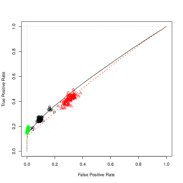
(a)

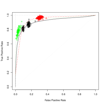
(b)

Figure 2: TPR vs FPR for $p=60$. The solid, dashed and dotted lines are the average TPR and FPR values for CLIME, Glasso and SCAD respectively as the tuning parameters of these methods vary. The circles, triangles and pluses correspond to $100$ different realizations of CLIME, Glasso and SCAD respectively, with the tuning parameter picked by cross validation.

To better illustrate the recovery performance elementwise, the heatmaps of the nonzeros identified out of $100$ replications are pictured in Figure 3. All the heatmaps suggest that CLIME is more sparse than Glasso, and by visual inspection the sparsity pattern recovered by CLIME has significantly better resemblance to the true model than Glasso. When the true model has significant nonzero elements scattered on the off diagonals, Glasso tends to include more nonzero elements than needed. SCAD produces the most sparse among the three but could again zero out more true nonzero entries as shown in Model 1. Similar patterns are observed in our experiments for other values of $p$.

Model 1
                             
Model 2

(a)

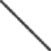
(b)

(c)

(d)

(e)

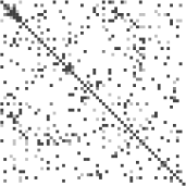
(f)

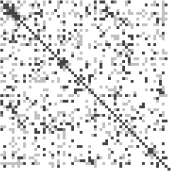
(g)

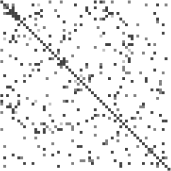
(h)

Figure 3: Heatmaps of the frequency of the zeros identified for each entry of the precision matrix (when $p=60$) out of $100$ replications. White color is $100$ zeros identified out of $100$ runs, and black is $0/100$.

5.2 Analysis of a breast cancer dataset

We now apply our method CLIME on a real data example. The breast cancer data were analyzed by Hess et al. (2006) and are available at
http://bioinformatics.mdanderson.org/. The data set consists of $22283$ gene expression levels of $133$ subjects, $34$ of which have achieved pathological complete response (pCR) and the rest with residual disease (RD). The pCR subjects are considered to have high chance of cancer-free survival in the long term, and thus it is of great interest to study the response states of the patients (pCR or RD) to neoadjuvant (preoperative) chemotherapy. Based on the estimated inverse covariance matrix of the gene expression levels, we apply the linear discriminant analysis (LDA) to predict whether a subject can achieve the pCR state or not.

For a fair comparison with other methods on estimating the inverse covariance matrix, we follow the same analysis scheme discussed in Fan et al. (2009) and the references therein. For completeness, we here give a brief description of these steps. The data are randomly divided into the training and the testing data sets. A stratified sampling approach is applied to divide the data, where $5$ pCR subjects and $16$ RD subjects are randomly selected to constitute the testing data (roughly $1/6$ of the subjects in each group). The remaining subjects form the training set. On the training set, a two sample $t$ test is performed between the two groups for each gene, and the $113$ most significant genes (smallest $p$-values) are retained as the covariates for prediction. Note that the size of the training sample is $112$, one less than the variable size, hence it allows us to examine the performance when $p>n$. The gene data are then standardized by the estimated standard deviation, estimated from the training data. Finally, following the LDA framework, the normalized gene expression data are assumed to be normally distributed as $N(\boldsymbol{\mu}_{k},\boldsymbol{\Sigma})$, where the two groups are assumed to have the same covariance matrix $\boldsymbol{\Sigma}$ but different means $\boldsymbol{\mu}_{k}$, $k=1$ for pCR and $k=2$ for RD. The estimated inverse covariance $\hat{\boldsymbol{\Omega}}$ produced by different methods is used in the linear discriminant scores

$$\delta_{k}(\boldsymbol{x})=\boldsymbol{x}^{T}\hat{\boldsymbol{\Omega}}\hat{\boldsymbol{\mu}}_{k}-\frac{1}{2}\hat{\boldsymbol{\mu}}_{k}^{T}\hat{\boldsymbol{\Omega}}\hat{\boldsymbol{\mu}}_{k}+\log\hat{\pi}_{k},$$ (20)

where $\hat{\pi}_{k}=n_{k}/n$ is the proportion of group $k$ subjects in the training set and $\hat{\boldsymbol{\mu}}_{k}=(1/n_{k})\sum_{i\in\text{group }k}\boldsymbol{x}_{i}$ is the within-group average vector in the training set. The classification rule is taken to be $\hat{k}(\boldsymbol{x})=\mathop{\rm arg\max}\delta_{k}(\boldsymbol{x})$ for $k=1,2$.

The classification performance is clearly associated with the estimation accuracy of $\hat{\boldsymbol{\Omega}}$. We use the testing data set to assess the estimation performance and compare with the existing results in Fan et al. (2009) using the same criterion. For the tuning parameters, we use a $6$ fold cross validation on the training data for picking $\lambda$. The above estimation scheme is repeated $100$ times.

To compare the classification performance, specificity, sensitivity and Mathews Correlation Coefficient (MCC) criteria are used, which are defined as follows:

$$\text{Specificity}=\frac{\text{TN}}{\text{TN}+\text{FP}},\quad\text{Sensitivity}=\frac{\text{TP}}{\text{TP}+\text{FN}},$$

$$\text{MCC}=\frac{\text{TP}\times\text{TN}-\text{FP}\times\text{FN}}{\sqrt{(\text{TP}+\text{FP})(\text{TP}+\text{FN})(\text{TN}+\text{FP})(\text{TN}+\text{FN})}},$$

where TP and TN stand for true positives (pCR) and true negatives (RD) respectively, and FP and FN for false positives/negatives. The larger the criterion value, the better the classification performance. The averages and standard errors of the above criteria along with the number of nonzero entries in $\hat{\boldsymbol{\Omega}}$ over $100$ replications are reported in Table 4. The Glasso, Adaptive lasso and SCAD results are taken from Fan et al. (2009), which uses the same procedure on the same data set, except that we here use $\hat{\boldsymbol{\Omega}}_{\rm CLIME}$ in place of $\hat{\boldsymbol{\Omega}}$.

Table 4: Comparison of average(SE) pCR classification errors over $100$ replications. Glasso, Adaptive lasso and SCAD results are taken from Fan et al. (2009), Table 2.

Method	Specificity	Sensitivity	MCC	Nonzero entries in $\hat{\boldsymbol{\Omega}}$
Glasso	$0.768(0.009)$	$0.630(0.021)$	$0.366(0.018)$	$3923(2)$
Adaptive lasso	$0.787(0.009)$	$0.622(0.022)$	$0.381(0.018)$	$1233(1)$
SCAD	$0.794(0.009)$	$0.634(0.022)$	$0.402(0.020)$	$674(1)$
CLIME	$0.749(0.005)$	$0.806(0.017)$	$0.506(0.020)$	$492(7)$

It is clear that CLIME significantly outperforms on the sensitivity and is comparable with other two methods on the specificity. The overall classification performance measured by MCC overwhelmingly favors our method CLIME, which shows an $25\%$ improvement over the best alternative methods. CLIME also produced the most sparse matrix than all other alternatives, which is usually favorable for interpretation purposes on real data sets.

6 Discussion

This paper develops a new constrained $\ell_{1}$ minimization method for estimating high dimensional precision matrices. Both the method and the analysis are relatively simple and straightforward, and may be extended to other related problems. Moreover, the method and the results are not restricted to a specific sparsity pattern. Thus the estimator can be used to recover a wide class of matrices in theory as well as in applications. In particular, when applying our method to covariance selection in Gaussian graphical models, the theoretical results can be established without assuming the irrepresentable condition in Ravikumar et al. (2008), which is very stringent and hard to check in practice.

Several papers, such as Yuan and Lin (2007), Rothman et al.  (2008) and Ravikumar et al. (2008), estimate the precision matrix by solving the optimization problem (16) with $\ell_{1}$ penalty only on the off diagonal entries, which is slightly different from our starting point (4) presented here. One can also similarly considered the following optimization problem

$$\min\|\boldsymbol{\Omega}\|_{1,\rm off}~{}~{}\mbox{subj}~{}~{}|\boldsymbol{\Sigma}_{n}\boldsymbol{\Omega}-\boldsymbol{I}|_{\infty}\leq\lambda_{n},~{}~{}\boldsymbol{\Omega}\in I\!\!R^{p\times p}.$$

Analogous results can also be established for the above estimator. We omit them in this paper, due to high resemblance in proof techniques and conclusions.

There are several possible extensions for our method. For example, Zhou et al. (2008) considered the time varying undirected graphs and estimated $\boldsymbol{\Sigma}(t)^{-1}$ by Glasso. It would be very interesting to study the estimation of $\boldsymbol{\Sigma}(t)^{-1}$ by our method. Ravikumar and Wainwright (2009) considered high-dimensional Ising model selection using $\ell_{1}$-regularized logistic regression. It would be interesting to apply our method to their setting as well.

Another important subject is to investigate the theoretical property of the tuning parameter selected by cross-validation method, though from our experiments CLIME is not very sensitive to the choice of the tuning parameter. An example of such results on cross validation can be found in Bickel and Levina (2008b) on thresholding.

After this paper was submitted, it came to our attention that Zhang (2010) proposed a precision matrix estimator, called GMACS, which is the solution of the following optimization problem:

$$\min\|\boldsymbol{\Omega}\|_{L_{1}}~{}~{}\mbox{subject to:}~{}~{}|\boldsymbol{\Sigma}_{n}\boldsymbol{\Omega}-\boldsymbol{I}|_{\infty}\leq\lambda_{n},~{}~{}\boldsymbol{\Omega}\in I\!\!R^{p\times p}.$$

The objective function here is different from that of CLIME, and this basic version cannot be solved column by column and is not as easy to implement. Zhang (2010) considers only the Gaussian case and $\ell_{0}$ balls, whereas we consider subgaussian and polynomial-tail distributions and more general $\ell_{q}$ balls. Also, the GMACS estimator requires an additional thresholding step in order for the rates to hold over $\ell_{0}$ balls. In contrast, CLIME does not need an additional thresholding step and the rates hold over general $\ell_{q}$ balls.

7 Proof of Main Results

Proof of Lemma 1. Write $\boldsymbol{\Omega}=(\boldsymbol{\omega}_{1},\dotsc,\boldsymbol{\omega}_{p})$, where $\boldsymbol{\omega}_{i}\in I\!\!R^{p}$. The constraint $|\boldsymbol{\Sigma}_{n}\boldsymbol{\Omega}-\boldsymbol{I}|_{\infty}\leq\lambda_{n}$ is equivalent to

$$|\boldsymbol{\Sigma}_{n}\boldsymbol{\omega}_{i}-\boldsymbol{e}_{i}|_{\infty}\leq\lambda_{n}~{}~{}\mbox{for~{}~{}}1\leq i\leq p.$$

Thus we have

$$|\hat{\boldsymbol{\omega}}^{1}_{i}|_{1}\geq|\hat{\boldsymbol{\beta}}_{i}|_{1}~{}~{}\mbox{for $1\leq i\leq p$.}$$ (21)

Since $|\boldsymbol{\Sigma}_{n}\hat{\textbf{B}}-\boldsymbol{I}|_{\infty}\leq\lambda_{n}$, by the definitions of $\{\hat{\boldsymbol{\Omega}}_{1}\}$, we have

$$\|\hat{\boldsymbol{\Omega}}_{1}\|_{1}\leq\|\hat{\textbf{B}}\|_{1}.$$ (22)

By(21) and (22), we have $\hat{\textbf{B}}\in\{\hat{\boldsymbol{\Omega}}_{1}\}$. On the other hand, if $\hat{\boldsymbol{\Omega}}_{1}\notin\{\hat{\textbf{B}}\}$, then there exists an $i$ such that $|\hat{\boldsymbol{\omega}}_{i}|_{1}>|\hat{\boldsymbol{\beta}}_{i}|_{1}$. Hence by (21) we have $\|\hat{\boldsymbol{\Omega}}_{1}\|_{1}>\|\hat{\textbf{B}}\|_{1}$. This is in conflict with (22).  

The main results all rely on Theorem 6, which upper bounds the elementwise $\ell_{\infty}$ norm. We will prove it first.

Proof of Theorem 6. Let $\hat{\boldsymbol{\beta}}_{i,\rho}$ be a solution of (3) by replacing $\boldsymbol{\Sigma}_{n}$ with $\boldsymbol{\Sigma}_{n,\rho}$. Note that Lemma 1 still holds for $\hat{\boldsymbol{\Omega}}_{n,\rho}$ and $\{\hat{\boldsymbol{\beta}}_{i,\rho}\}$ with $\rho\geq 0$. For notation briefness, we only prove the theorem for $\rho=0$. The proof is exactly the same for general $\rho>0$. By the condition in Theorem 6,

$$|\boldsymbol{\Sigma}_{0}-\boldsymbol{\Sigma}_{n}|_{\infty}\leq\lambda_{n}/\|\boldsymbol{\Omega}_{0}\|_{L_{1}}.$$ (23)

Then we have

$$|\boldsymbol{I}-\boldsymbol{\Sigma}_{n}\boldsymbol{\Omega}_{0}|_{\infty}=|(\boldsymbol{\Sigma}_{0}-\boldsymbol{\Sigma}_{n})\boldsymbol{\Omega}_{0}|_{\infty}\leq\|\boldsymbol{\Omega}_{0}\|_{L_{1}}|\boldsymbol{\Sigma}_{0}-\boldsymbol{\Sigma}_{n}|_{\infty}\leq\lambda_{n},$$ (24)

where we used the inequality $|\boldsymbol{A}\boldsymbol{B}|_{\infty}\leq|\boldsymbol{A}|_{\infty}\|\boldsymbol{B}\|_{L_{1}}$ for matrices $\boldsymbol{A},\boldsymbol{B}$ of appropriate sizes. By the definition of $\hat{\boldsymbol{\beta}}_{i}$, we can see that $|\hat{\boldsymbol{\beta}}_{i}|_{1}\leq\|\boldsymbol{\Omega}_{0}\|_{L_{1}}$ for $1\leq i\leq p$. By Lemma 1,

$$\|\hat{\boldsymbol{\Omega}}_{1}\|_{L_{1}}\leq\|\boldsymbol{\Omega}_{0}\|_{L_{1}}.$$ (25)

We have

$$|\boldsymbol{\Sigma}_{n}(\hat{\boldsymbol{\Omega}}_{1}-\boldsymbol{\Omega}_{0})|_{\infty}\leq|\boldsymbol{\Sigma}_{n}\hat{\boldsymbol{\Omega}}_{1}-\boldsymbol{I}|_{\infty}+|\boldsymbol{I}-\boldsymbol{\Sigma}_{n}\boldsymbol{\Omega}_{0}|_{\infty}\leq 2\lambda_{n}.$$ (26)

Therefore by (23)-(26),

$$|\boldsymbol{\Sigma}_{0}(\hat{\boldsymbol{\Omega}}_{1}-\boldsymbol{\Omega}_{0})|_{\infty} \leq |\boldsymbol{\Sigma}_{n}(\hat{\boldsymbol{\Omega}}_{1}-\boldsymbol{\Omega}_{0})|_{\infty}+|(\boldsymbol{\Sigma}_{n}-\boldsymbol{\Sigma}_{0})(\hat{\boldsymbol{\Omega}}_{1}-\boldsymbol{\Omega}_{0})|_{\infty}$$

$$\leq 2\lambda_{n}+\|\hat{\boldsymbol{\Omega}}_{1}-\boldsymbol{\Omega}_{0}\|_{L_{1}}|\boldsymbol{\Sigma}_{n}-\boldsymbol{\Sigma}_{0}|_{\infty}\leq 4\lambda_{n}.$$

It follows that

$$|\hat{\boldsymbol{\Omega}}_{1}-\boldsymbol{\Omega}_{0}|_{\infty}\leq\|\boldsymbol{\Omega}_{0}\|_{L_{1}}|\boldsymbol{\Sigma}_{0}(\hat{\boldsymbol{\Omega}}_{1}-\boldsymbol{\Omega}_{0})|_{\infty}\leq 4\|\boldsymbol{\Omega}_{0}\|_{L_{1}}\lambda_{n}.$$

This establishes (13) by the definition in (2).

We next prove (14). Let $t_{n}=|\hat{\boldsymbol{\Omega}}-\boldsymbol{\Omega}_{0}|_{\infty}$ and define

$$\boldsymbol{h}_{j}=\hat{\boldsymbol{\omega}}_{j}-\boldsymbol{\omega}^{0}_{j},$$

$$\boldsymbol{h}^{1}_{j}=(\hat{\boldsymbol{\omega}}_{ij}I\{|\hat{{{\omega}}}_{ij}|\geq 2t_{n}\};1\leq i\leq p)^{T}-\boldsymbol{\omega}^{0}_{j},~{}~{}\boldsymbol{h}^{2}_{j}=\boldsymbol{h}_{j}-\boldsymbol{h}^{1}_{j}.$$

By the definition (2) of $\hat{\boldsymbol{\Omega}}$, we have $|\hat{\boldsymbol{\omega}}_{j}|_{1}\leq|\hat{\boldsymbol{\omega}}^{1}_{j}|_{1}\leq|\boldsymbol{\omega}^{0}_{j}|_{1}$. Then

$$|\boldsymbol{\omega}^{0}_{j}|_{1}-|\boldsymbol{h}^{1}_{j}|_{1}+|\boldsymbol{h}^{2}_{j}|_{1}\leq|\boldsymbol{\omega}^{0}_{j}+\boldsymbol{h}^{1}_{j}|_{1}+|\boldsymbol{h}^{2}_{j}|_{1}=|\hat{\boldsymbol{\omega}}_{j}|_{1}\leq|\boldsymbol{\omega}^{0}_{j}|_{1},$$

which implies that $|\boldsymbol{h}^{2}_{j}|_{1}\leq|\boldsymbol{h}^{1}_{j}|_{1}$. This follows that $|\boldsymbol{h}_{j}|_{1}\leq 2|\boldsymbol{h}^{1}_{j}|_{1}$. So we only need to upper bound $|\boldsymbol{h}^{1}_{j}|_{1}$. We have

$$|\boldsymbol{h}^{1}_{j}|_{1} = \sum_{i=1}^{p}|\hat{\omega}_{ij}I\{|\hat{\omega}_{ij}|\geq 2t_{n}\}-\omega^{0}_{ij}|$$ (27)

$$\leq \sum_{i=1}^{p}|\omega^{0}_{ij}I\{|\omega^{0}_{ij}|\leq 2t_{n}\}|+\sum_{i=1}^{p}|\hat{\omega}_{ij}I\{|\hat{\omega}_{ij}|\geq 2t_{n}\}-\omega^{0}_{ij}I\{|\omega^{0}_{ij}|\geq 2t_{n}\}|$$ (28)

$$\leq (2t_{n})^{1-q}s_{0}(p)+t_{n}\sum_{i=1}^{p}I\{|\hat{\omega}_{ij}|\geq 2t_{n}\}+\sum_{i=1}^{p}|\omega^{0}_{ij}||I\{|\hat{\omega}_{ij}|\geq 2t_{n}\}-I\{|\omega^{0}_{ij}|\geq 2t_{n}\}|$$ (29)

$$\leq (2t_{n})^{1-q}s_{0}(p)+t_{n}\sum_{i=1}^{p}I\{|\omega^{0}_{ij}|\geq t_{n}\}+\sum_{i=1}^{p}|\omega^{0}_{ij}|I\{||\omega^{0}_{ij}|-2t_{n}|\leq|\hat{\omega}_{ij}-\omega^{0}_{ij}|\}$$ (30)

$$\leq (2t_{n})^{1-q}s_{0}(p)+(t_{n})^{1-q}s_{0}(p)+(3t_{n})^{1-q}s_{0}(p)$$ (31)

$$\leq (1+2^{1-q}+3^{1-q})t_{n}^{1-q}s_{0}(p),$$ (32)

where we used the following inequality: for any $a,b,c\in I\!\!R$, we have

$$|I\{a<c\}-I\{b<c\}|\leq I\{|b-c|<|a-b|\}.$$

This completes the proof of (14).

Finally, (15) follows from (27), (13) and the inequality $\|\boldsymbol{A}\|^{2}_{F}\leq p\|\boldsymbol{A}\|_{L_{1}}|\boldsymbol{A}|_{\infty}$ for any $p\times p$ matrix.  

Proof of Theorems 1 (i) and 4 (i). By Theorem 6, we only need to prove

$$\max_{ij}|\hat{\sigma}_{ij}-\sigma^{0}_{ij}|\leq C_{0}\sqrt{\log p/n}$$ (33)

with probability greater than $1-4p^{-\tau}$ under (C1). Without loss of generality, we assume $\textsf{E}\textbf{X}=0$. Let $\boldsymbol{\Sigma}^{0}_{n}:=n^{-1}\sum_{k=1}^{n}\textbf{X}_{k}\textbf{X}_{k}^{T}$ and $Y_{kij}=X_{ki}X_{kj}-\textsf{E}X_{ki}X_{kj}$. Then we have $\boldsymbol{\Sigma}_{n}=\boldsymbol{\Sigma}^{0}_{n}-\bar{\textbf{X}}\bar{\textbf{X}}^{T}$. Let $t=\eta\sqrt{\log p/n}$. Using the inequality $|e^{s}-1-s|\leq s^{2}e^{\max(s,0)}$ for any $s\in R$ and letting $C_{K1}=2+\tau+\eta^{-1}K^{2}$, by basic calculations, we can get

$$\textsf{P}\Big{(}\sum_{k=1}^{n}Y_{kij}\geq\eta^{-1}C_{K1}\sqrt{n\log p}\Big{)} \leq e^{-C_{K1}\log p}\Big{(}\textsf{E}\exp(tY_{kij})\Big{)}^{n}$$

$$\leq \exp\Big{(}-C_{K1}\log p+nt^{2}\textsf{E}Y^{2}_{kij}e^{t|Y_{kij}|}\Big{)}$$

$$\leq \exp\Big{(}-C_{K1}\log p+\eta^{-1}K^{2}\log p\Big{)}$$

$$\leq \exp(-(\tau+2)\log p).$$

Hence we have

$$\textsf{P}\Big{(}|\boldsymbol{\Sigma}^{0}_{n}-\boldsymbol{\Sigma}_{0}|_{\infty}\geq\eta^{-1}C_{K1}\sqrt{\log p/n}\Big{)}\leq 2p^{-\tau}.$$ (34)

By the simple inequality $e^{s}\leq e^{s^{2}+1}$ for $s>0$, we have $\textsf{E}e^{t|X_{j}|}\leq eK$ for all $t\leq\eta^{1/2}$. Let $C_{K2}=2+\tau+\eta^{-1}e^{2}K^{2}$ and $a_{n}=C^{2}_{K2}(\log p/n)^{1/2}$. As above, we can show that

$$\textsf{P}\Big{(}|\bar{\textbf{X}}\bar{\textbf{X}}^{T}|_{\infty}\geq\eta^{-2}a_{n}\sqrt{\log p/n}\Big{)} \leq p\max_{i}\textsf{P}\Big{(}\sum_{k=1}^{n}X_{ki}\geq\eta^{-1}C_{K2}\sqrt{n\log p}\Big{)}$$ (36)

$$+p\max_{i}\textsf{P}\Big{(}-\sum_{k=1}^{n}X_{ki}\geq\eta^{-1}C_{K2}\sqrt{n\log p}\Big{)}$$

$$\leq 2p^{-\tau-1}.$$ (37)

By (34), (36) and the inequality $C_{0}>\eta^{-1}C_{K1}+\eta^{-2}a_{n}$, we see that (33) holds.  

Proof of Theorems 1 (ii) and 4 (ii). Let

$$\bar{Y}_{kij}=X_{ki}X_{kj}I\{|X_{ki}X_{kj}|\leq\sqrt{n/(\log p)^{3}}\}-\textsf{E}X_{ki}X_{kj}I\{|X_{ki}X_{kj}|\leq\sqrt{n/(\log p)^{3}}\},$$

$$\check{Y}_{kij}=Y_{kij}-\bar{Y}_{kij}.$$

Since $b_{n}:=\max_{i,j}\textsf{E}|X_{ki}X_{kj}|I\{|X_{ki}X_{kj}|\geq\sqrt{n/(\log p)^{3}}\}=O(1)n^{-\gamma-1/2}$, we have by (C2),

$$\textsf{P}\Big{(}\max_{i,j}|\sum_{k=1}^{n}\check{Y}_{kij}|\geq 2nb_{n}\Big{)}$$

$$\leq\textsf{P}\Big{(}\max_{i,j}|\sum_{k=1}^{n}X_{ki}X_{kj}I\{|X_{ki}X_{kj}|>\sqrt{n/(\log p)^{3}}\}|\geq nb_{n}\Big{)}$$

$$\leq\textsf{P}\Big{(}\max_{i,j}\sum_{k=1}^{n}|X_{ki}X_{kj}|I\{X^{2}_{ki}+X^{2}_{kj}\geq 2\sqrt{n/(\log p)^{3}}\}\geq nb_{n}\Big{)}$$

$$\leq\textsf{P}\Big{(}\max_{k,i}X_{ki}^{2}\geq\sqrt{n/(\log p)^{3}}\Big{)}$$

$$\leq pn\textsf{P}\Big{(}X^{2}_{1}\geq\sqrt{n/(\log p)^{3}}\Big{)}$$

$$=O(1)n^{-\delta/8}.$$

By Bernstein’s inequality (cf. Bennett (1962)) and some elementary calculations,

$$\textsf{P}\Big{(}\max_{i,j}|\sum_{k=1}^{n}\bar{Y}_{kij}|\geq\sqrt{(\theta+1)(4+\tau)n\log p}\Big{)}$$

$$\leq p^{2}\max_{i,j}\textsf{P}\Big{(}|\sum_{k=1}^{n}\bar{Y}_{kij}|\geq\sqrt{(\theta+1)(4+\tau)n\log p}\Big{)}$$

$$\leq 2p^{2}\max_{i,j}\exp\Big{(}-\frac{(\theta+1)(4+\tau)n\log p}{2n\textsf{E}\bar{Y}^{2}_{1ij}+\sqrt{(\theta+1)(64+16\tau)}n/(3\log p)}\Big{)}$$

$$=O(1)p^{-\tau/2}.$$

So we have

$$\textsf{P}\Big{(}|\boldsymbol{\Sigma}^{0}_{n}-\boldsymbol{\Sigma}_{0}|_{\infty}\geq\sqrt{(\theta+1)(4+\tau)\log p/n}+2b_{n}\Big{)}=O\Big{(}n^{-\delta/8}+p^{-\tau/2}\Big{)}.$$ (38)

Using the same truncation argument and Bernstein’s inequality, we can show that

$$\textsf{P}\Big{(}\max_{i}\Big{|}\sum_{k=1}^{n}X_{ki}\Big{|}\geq\sqrt{\max_{i}\sigma^{0}_{ii}(4+\tau)n\log p}\Big{)}=O\Big{(}n^{-\delta/8}+p^{-\tau/2}\Big{)}.$$

Hence

$$\textsf{P}\Big{(}|\bar{\textbf{X}}\bar{\textbf{X}}^{T}|_{\infty}\geq\max_{i}\sigma^{0}_{ii}(4+\tau)\log p/n\Big{)}=O\Big{(}n^{-\delta/8}+p^{-\tau/2}\Big{)}.$$ (39)

Combining (38) and (39), we have

$$\max_{ij}|\hat{\sigma}_{ij}-\sigma^{0}_{ij}|\leq\sqrt{(\theta+1)(5+\tau)\log p/n}$$ (40)

with probability greater than $1-O\Big{(}n^{-\delta/8}+p^{-\tau/2}\Big{)}$. The proof is completed by (40) and Theorem 6.   

Proof of Theorems 2 and 5. Since $\boldsymbol{\Sigma}^{-1}_{n,\rho}$ is a feasible point, we have by (10),

$$\|\hat{\boldsymbol{\Omega}}_{\rho}\|_{1}\leq\|\hat{\boldsymbol{\Omega}}_{1\rho}\|_{1}\leq\|\boldsymbol{\Sigma}^{-1}_{n,\rho}\|_{1}\leq p^{2}\max(\sqrt{\frac{n}{\log p}},p^{\alpha}).$$

By (33), Theorem 6, the fact $p\geq n^{\xi}$ and since $\tau$ is large enough, we have

$$\sup_{\boldsymbol{\Omega}_{0}\in\mathcal{U}}\textsf{E}\|\hat{\boldsymbol{\Omega}}_{\rho}-\boldsymbol{\Omega}_{0}\|^{2}_{2} = \sup_{\boldsymbol{\Omega}_{0}\in\mathcal{U}}\textsf{E}\|\hat{\boldsymbol{\Omega}}_{\rho}-\boldsymbol{\Omega}_{0}\|^{2}_{2}I\{\max_{ij}|\hat{\sigma}_{ij}-\sigma^{0}_{ij}|+\rho\leq C_{0}\sqrt{\log p/n}\}$$

$$+\sup_{\boldsymbol{\Omega}_{0}\in\mathcal{U}}\textsf{E}\|\hat{\boldsymbol{\Omega}}_{\rho}-\boldsymbol{\Omega}_{0}\|^{2}_{2}I\{\max_{ij}|\hat{\sigma}_{ij}-\sigma^{0}_{ij}|+\rho>C_{0}\sqrt{\log p/n}\}$$

$$= O\Big{(}M^{4-4q}s^{2}_{0}(p)\Big{(}\frac{\log p}{n}\Big{)}^{1-q}\Big{)}+O\Big{(}p^{4}\max(\frac{n}{\log p},p^{2\alpha})p^{-\tau/2}\Big{)}$$

$$= O\Big{(}M^{4-4q}s^{2}_{0}(p)\Big{(}\frac{\log p}{n}\Big{)}^{1-q}\Big{)}.$$

This proves Theorem 2. The proof of Theorem 5 is similar.  

Proof of Theorem 3. Let $k_{n}$ be an integer satisfying $1\leq k_{n}\leq n$. Define

$$\boldsymbol{h}_{j}=\hat{\boldsymbol{\omega}}_{j}-\boldsymbol{\omega}^{0}_{j},$$

$$\boldsymbol{h}^{1}_{j}=(\hat{\omega}_{ij}I\{1\leq i\leq k_{n}\};1\leq i\leq p)^{T}-\boldsymbol{\omega}^{0}_{j},~{}~{}\boldsymbol{h}^{2}_{j}=\boldsymbol{h}_{j}-\boldsymbol{h}^{1}_{j}.$$

By the proof of Theorem 6, we can show that $|\boldsymbol{h}_{j}|_{1}\leq 2|\boldsymbol{h}^{1}_{j}|_{1}$. Since $\boldsymbol{\Omega}_{0}\in\mathcal{U}_{o}(\alpha,M)$, we have $\sum_{j\geq k_{n}}|\omega^{0}_{ij}|\leq Mk^{-\alpha}_{n}$. By Theorem 4, $\sum_{j=1}^{k_{n}}|\hat{\omega}_{ij}-\omega^{0}_{ij}|=O\Big{(}k_{n}\sqrt{\log p/n}\Big{)}$ with probability greater than $1-O\Big{(}n^{-\delta/8}+p^{-\tau/2}\Big{)}$. Theorem 3 (i) is proved by taking $k_{n}=[(n/\log p)^{1/(2\alpha+2)}]$. The proof of Theorem 3 (ii) is similar as that of Theorem 2.

References

• [1] Banerjee, O., Ghaoui, L.E. and d’Aspremont, A. (2008). Model selection through sparse maximum likelihood estimation. Journal of Machine Learning Research 9: 485-516.
• [2] Bennett, G (1962). Probability inequalities for the sum of independent random variables. Journal of the American Statistical Association 57: 33-45.
• [3] Bickel, P. and Levina, E. (2008a). Regularized estimation of large covariance matrices. Annals of Statistics 36: 199-227.
• [4] Bickel, P. and Levina, E. (2008b). Covariance regularization by thresholding. Annals of Statistics 36: 2577-2604.
• [5] Boyd, S. and Vandenberghe, L (2004). Convex optimization. Cambridge University Press.
• [6] Cai, T., Zhang, C.-H. and Zhou, H. (2010). Optimal rates of convergence for covariance matrix estimation. Annals of Statistics 38: 2118-2144.
• [7] Cai, T., Wang, L. and Xu, G. (2010). Shifting inequality and recovery of sparse signals. IEEE Transactions on Signal Processing 58: 1300-1308.
• [8] Candès, E. and Tao, T. (2007). The Dantzig selector: statistical estimation when $p$ is much larger than $n$. Annals of Statistics 35: 2313-2351.
• [9] d’Aspremont, A., Banerjee, O., and El Ghaoui, L. (2008). First-order methods for sparse covariance selection. SIAM Journal on Matrix Analysis and its Applications 30: 56-66.
• [10] Fan, J. (1997). Comments on ’Wavelets in Statistics: A Review’ by A. Antoniadis Journal of the Italian Statistical Association 6: 131-138.
• [11] Fan, J., Feng, Y., and Wu, Y. (2009). Network exploration via the adaptive lasso and SCAD penalties. Annals of Applied Statistics 2: 521-541.
• [12] Fan, J. and Li, R. (2001). Variable selection via nonconcave penalized likelihood and its oracle properties. Journal of American Statistical Association 96: 1348-1360.
• [13] Friedman, J., Hastie, T. and Tibshirani, R. (2008). Sparse inverse covariance estimation with the graphical lasso. Biostatistics 9: 432-441.
• [14] Hess, K. R., Anderson, K., Symmans, W. F., Valero, V., Ibrahim, N., Mejia, J. A., Booser, D., Theriault, R. L., Buzdar, A. U., Dempsey, P. J., Rouzier, R., Sneige, N., Ross, J. S., Vidaurre, T., Gómez, H. L., Hortobagyi, G. N. and Pusztai, L. (2006). Pharmacogenomic predictor of sensitivity to preoperative chemotherapy with paclitaxel and fluorouracil, doxorubicin, and cyclophosphamide in breast cancer. Journal of Clinical Oncology 24: 4236-44.
• [15] Huang, J., Liu, N., Pourahmadi, M. and Liu, L. (2006). Covariance matrix selection and estimation via penalized normal likelihood. Biometrika 93: 85-98.
• [16] El Karoui, N. (2008). Operator norm consistent estimation of large-dimensional sparse covariance matrices. Annals of Statistics 36: 2717-2756.
• [17] Lam, C. and Fan, J. (2009). Sparsistency and rates of convergence in large covariance matrix estimation. Annals of Statistics 37: 4254-4278.
• [18] Lauritzen, S.L. (1996). Graphical models (Oxford statistical science series). Oxford University Press, USA.
• [19] Liu, H., Lafferty, J. and Wasserman, L. (2009). The nonparanormal: semiparametric estimation of high dimensional undirected graphs. Journal of Machine Learning Research. To appear.
• [20] Meinshausen, N. and Bühlmann, P. (2006). High-dimensional graphs and variable selection with the Lasso. Annals of Statistics 34: 1436-1462.
• [21] Ravikumar,P. and Wainwright, M. (2009). High-dimensional Ising model selection using $l_{1}$-regularized logistic regression. Annals of Statistics 38: 1287-1319.
• [22] Ravikumar, P., Wainwright, M., Raskutti, G. and Yu, B. (2008). High-dimensional covariance estimation by minimizing $l_{1}$-penalized log-determinant divergence. Technical Report 797, UC Berkeley, Statistics Department, Nov. 2008. (Submitted).
• [23] Rothman, A., Bickel, P., Levina, E. and Zhu, J. (2008). Sparse permutation invariant covariance estimation. Electronic Journal of Statistics 2: 494-515.
• [24] Wu, W.B. and Pourahmadi, M. (2003). Nonparametric estimation of large covariance matrices of longitudinal data. Biometrika 90: 831-844.
• [25] Yuan, M. (2009). Sparse inverse covariance matrix estimation via linear programming. Journal of Machine Learning Research 11: 2261-2286.
• [26] Yuan, M. and Lin, Y. (2007). Model selection and estimation in the Gaussian graphical model. Biometrika 94: 19-35.
• [27] Zhang, C. (2010). Estimation of large inverse matrices and graphical model selection. Technical Report, Rutgers University, Department of Statistics and Biostatistics.
• [28] Zhou, S., Lafferty, J. and Wasserman, L. (2008). Time varying undirected graphs. To appear in Machine Learning Journal (invited), special issue for the 21st Annual Conference on Learning Theory (COLT 2008).
• [29] Zhou, S., van de Geer, S. and Bühlmann, P. (2009). Adaptive lasso for high dimensional regression and Gaussian graphical modeling. Arxiv preprint arXiv:0903.2515.