Cofermion Theory for Pseudogap Phenomena and Superconducting Mechanism of Underdoped Cuprate Superconductors

Abstract

We study pseudogap phenomena and Fermi-arc formation experimentally observed in typical two dimensional doped Mott insulators, namely, underdoped cuprate superconductors. To develop a physically unequivocal theory, we start from the slave-boson mean-field theory for the Hubbard model on a square lattice. Our crucial step is to further take into account the charge dynamics and fluctuations. The extra charge fluctuations seriously modify low-energy single-particle spectra of doped Mott insulators near the Fermi level: An electron added around an empty site (or a hole added around a doubly occupied site) constitutes composite fermion (cofermion), called holo-electron (or doublo-hole) at low energy in distinction from the normal quasiparticles. These unexplored composite fermions substantiate the extra charge fluctuation. We show that the quasiparticles hybridize with the holo-electrons and doublo-holes. The resultant hybridization gap is identified as the pseudogap observed in the underdoped region of the high-$T_{{\rm c}}$ cuprates. Because the Fermi level crosses the top (bottom) of the low-energy band formed just below (above) the hybridization gap in the hole-doped (electron-doped) case, it causes a Fermi-surface reconstruction, namely, a topological change in the Fermi surface forced by the penetration of zeros of the quasiparticle Green function. This reconstruction signals the emergence of a non-Fermi-liquid phase. The pseudogap, and the resultant formation of pocket or arc of the Fermi surface reproduce the experimental results for the cuprate superconductors in the underdoped region. The pairing channel opens not only between two quasiparticles but also between a quasiparticle and a cofermion. This pairing solves the puzzle of the dichotomy between the $d$-wave superconductivity and the precursors of the the insulating gap in the antinodal region. We propose and analyze them as the mechanism of the high-temperature superconductivity for the cuprates.

I Introduction

The discovery of cuprate superconductors has triggered extensive studies on the nature of low-energy electronic excitations evolving in doped Mott insulators. The extensive interest on the doped Mott insulators exists because it must be directly related with the origin of the high temperature superconductivity itself.

From the early stage of the studies, experimental observations have indicated that quasiparticle states of normal phases of cuprates change qualitatively with the increase of the doping, together with changes in superconducting transition temperatures. It has been shownOng et al. (1987); Takagi et al. (1989) that the Hall coefficient $R_{H}$ changes its sign near the so-called optimal doping for the highest superconducting transition temperatures, followed by a steep increase of its amplitude $|R_{H}|$ with lowering doping concentration, typically indicating a drastic change in low-energy quasiparticles of the normal state between the underdoped and overdoped regions. Such a drastic change is also but differently suggested from observations of pseudogap phenomenaYasuoka et al. (1989); Rossat-Mignod et al. (1991); Loram et al. (1993); Homes et al. (1993); Nishikawa et al. (1993); Marshall et al. (1996), where the spin and charge excitations are unexpectedly suppressed in the underdoped region. Various types of non-Fermi-liquid properties are accompanied in this region.

Recent improved experimental tools have enabled resolving low-energy single-particle spectra near the Fermi level. In particular, strongly momentum-dependent quasiparticle states in the hole-underdoped cupratesDamascelli et al. (2003); Yoshida et al. (2006) observed by angle-resolved photoemission spectroscopy (ARPES) studies have renewed the interest in the low-energy spectrum of the cuprate superconductors. In contrast to the overdoped region, where a large Fermi surface crossing the region around the so-called antinodal points $(\pm\pi,0)$ and $(0,\pm\pi)$ in the 2D Brillouin zone for the CuO₂ plane is clearly observed, low-energy quasiparticle states around the antinodal points are missing in the underdoped cuprates. It emerges as a truncation of the large Fermi surface observed in the overdoped region. The resultant truncated structure is called the “Fermi arc”.

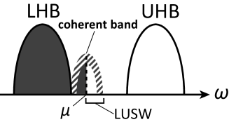
Figure 1: Schematic global density of states of hole-doped Mott insulators. The coherent band around the Fermi level $\mu$, the upper Hubbard band (UHB), and the lower Hubbard band (LHB) are schematically illustrated. The low-energy unoccupied spectral weight (LUSW) is also indicated.

From more fundamental point of view, the normal state of the cuprates offers a challenge of condensed matter physics as a typical open issue of “Mott physics”, namely, nature of strongly correlated metals in the proximity to the Mott insulatorPeierls (1937); Mott (1937); Imada et al. (1998). The experimentally observed arc-like Fermi surface in the underdoped cuprates is a hallmark of the proximity to the Mott insulators. As we illustrate in Fig.1, global energy spectra of doped Mott insulators are known to consist of essentially three energy “bands”; a coherent band around the Fermi level $\mu$ and two incoherent bands, namely, the upper Hubbard band (UHB) located above $\mu$, and the lower Hubbard band (LHB) located below $\mu$. For the hole-doped (electron-doped) systems, the coherent band is formed around the top of the LHB (the bottom of the UHB). The spectral weight formed just above (below) $\mu$ within the coherent band is often called the low-energy unoccupied spectral weight (LUSW) in the hole-doped (electron-doped) Mott insulators.

Such a global structure of spectra can be roughly described by a simple picture given by the dynamical mean-field theoryGeorges et al. (1996). It has unified two scenarios of earlier studies by HubbardHubbard (1964), and Brinkman and RiceBrinkman and Rice (1970) based on the Gutzwiller approximationGutzwiller (1965). The Hubbard approximation captures the formation of UHB and LHB. In the Brinkman-Rice picture, Mott insulators appear as a consequence of homogeneous vanishing of the quasiparticle weight uniformly on the Fermi surface. Therefore, this approximation draws a picture that quasiparticles are renormalized in a momentum-independent fashion and the effective mass diverges independently of the momentum position on the Fermi surface on the verge of the Mott transition.

In infinite-dimensional systems, such a route of the Mott transition has turned out to be correctMetzner and Vollhardt (1989); M${\rm\ddot{u}}$ller-Hartmann (1989); Georges et al. (1996). However, in finite dimensions, this picture has turned out to be too simple to understand the low-energy spectra and the nature of the Mott transition: Realistic theory has to capture significant momentum-dependent quasiparticle renormalization, as has been experimentally observed as Fermi-arc formation in the underdoped cuprates, and has also been revealed from various numerical attemptsImada and Onoda (2001); Onoda and Imada (2002); S${\rm\acute{e}}$n${\rm\acute{e}}$chal and Tremblay (2004); Stanescu and Kotliar (2006); Zhang and Imada (2007); Sakai et al. (2009, 2010). It has now become increasingly clear that a conceptually new idea for describing Mott physics including an emergence of the new non-Fermi-liquid phase in the underdoped region is desired.

In this paper, we extend our previous attemptYamaji and Imada (2011) for describing the momentum-dependent Mott physics including the mechanism of Mott transitions at the level of LUSW and for understanding the experimentally supported dramatic change in the electronic states of the cuprates. We give a detailed comparison with experiments and a novel superconducting mechanism based on the previous attemptYamaji and Imada (2011), together with the derivation of our theoretical description in details. We particularly pay attention to the possible reconstruction of the Fermi surface. If the reconstruction emerges, the doped Mott insulator becomes topologically inequivalent to the conventional Fermi liquid and hence offers an unexplored avenue for long-sort issue of unconventional metals.

In the present work, we propose a simple and physically transparent theory that accounts for the strongly momentum-dependent renormalization experimentally suggested in the cuprate superconductors. We focus on charge dynamics involved in the low-energy spectra of the doped Mott insulators. A key idea is that, near the Mott insulator, an electron (a hole) added to an empty (a doubly occupied) site costs much smaller energy than an electron (a hole) added to singly occupied sites and behaves as a component of a band separated from the main quasiparticle. Then near the Mott insulator, this separated excitation contributes to the LUSW in the hole-doped (electron-doped) Mott insulators. This is in contrast with the weakly correlated regime, in which an added electron (hole) constitutes a uniform excitation irrespective of the added site, because the added electron becomes uniformly and spatially extended with a good wavenumber of the momentum. In our theory, such an electron (a hole) added to an empty site (a doubly occupied site) forms a composite fermionic excitation (or cofermion), which we call holo-electron (doublo-hole). The conventional quasiparticles may be scattered by the doubly occupied site (empty site) and are transformed to the cofermions, which introduces finite life time into the quasiparticles. This scattering and transformation may alternatively be formulated as the hybridization between the conventional quasiparticles and the holo-electrons and/or doublo-holes. This hybridization naturally generates a hybridization gap and the resultant band splitting causes the Fermi-surface reconstructions, namely, topological changes in the Fermi surface. The hybridization gap and the topological change account for the experimentally suggested pseudogap and Fermi-arc formation, respectively, in the cuprates. Our unique prediction is that the pseudogap is independent of the precursor of the Mott gap itself, while the pseudogap has the structure of the $s$-wave type symmetry rather than the $d$-wave symmetry. In addition, the pseudogap identified here is in clear distinction from the superconducting gap as well. We propose several experimental tests to prove or disprove our theoretical consequences.

A way to understand topological changes in the Fermi surface has recently been proposed to originate from the emergence of zeros of single particle Green’s functions, which are the points in the $(k,\omega)$-space satisfying ${\rm Re}\ G(k,\omega)=0$ for the momentum $k$ and the frequency $\omega$. In other words, the single particle self-energy $\Sigma(k,\omega)$ diverges at the zeros of Green’s function. The idea of the emergence of the zeros has a root in the work by Dzyaloshinskii, who examined a possible extension of the Luttinger theorem into Mott insulating statesDzyaloshinskii (2003). As is reviewed in Ref.Rice, 2005, this idea is applied to the doped Mott insulators to explain the “Fermi arcs” observed by ARPES. Recent results of numerical calculations also suggest that the zeros emerging in doped Mott insulators reconstruct the Fermi surface and changes its topologyStanescu and Kotliar (2006); Sakai et al. (2009, 2010). Such a topological change is indeed claimed in a recent ARPES measurementMeng et al. (2009).

The Fermi surface reconstruction itself is not an unconventional phenomenon, if it accompanies a spontaneous symmetry breaking such as an antiferromagnetic order. In translational-symmetry broken phases with an ordering wavenumber $Q$, electrons with momentum $k$ hybridize, at least, with electrons at momentum $k+Q$. Then Fermi surface reconstructions are naturally understood as a consequence of the hybridization gap as we will discuss later in detail. It is indeed able to account for the formation of Fermi pockets or arc-like Fermi surfaces if a hybridization with other Fermionic excitations exist.

However, in the hole-doped cuprates, in spite of recent reports on time reversal symmetryFauqu${\rm\acute{e}}$ et al. (2006); Xia et al. (2008); Li et al. (2008) and rotational symmetryDaou et al. (2010) breakings in some of the cuprate superconductors, translational symmetry breakings have not been universally observedMacDougall et al. (2008). On the other hand, the “Fermi arc h or the truncated Fermi surface have universally been experimentally observed in the underdoped cuprates. To have a unified picture of the Mott physics, it is important to understand whether the Fermi surface reconstruction occurs as a consequence of the hybridization gap generated by the “hybridization” with some hidden fermionic excitations without assuming a symmetry broken phase. In the present theory, the hybridization between the conventional quasiparticles and the emergent fermionic excitations called the holo-electron and the doublo-hole naturally explain such a Fermi-surface reconstruction.

Now we go into some details regarding characteristic low-energy spectra of doped Mott insulators. As is proposed by Meinders, Eskes and SawatzkyMeinders et al. (1993), the doping dependence of the LUSW formed just above $\mu$, has a marked feature for nearly Mott insulating, correlated electron systems. As we have mentioned above, an electron added to a singly occupied site inevitably costs the on-site Coulomb interaction $U$ and gives an excitation in the UHB, whereas electrons added to empty sites exclusively contribute to the low-energy states just above $\mu$. Here, an empty site can accept an electron irrespective of its spin state and creates two unoccupied states, namely up and down spin states. Therefore the $N_{{\rm h}}$ holes create $N_{{\rm h}}$ empty sites in the atomic limit, where the kinetic energy of electrons $t$ is zero. Then, they create $2N_{{\rm h}}$ unoccupied states as a consequence. When the kinetic energy of the electrons $t$ becomes nonzero, the number of unoccupied states increases because of the pair creation of doubly occupied and empty sites induced by the hopping of electrons and resultant charge fluctuations. Therefore, for hole-doping concentration $x=N_{{\rm h}}/N_{{\rm s}}$ with $N_{{\rm s}}$ being the total number of lattice sites, the LUSW in the doped Mott insulator is always larger than $2x$. From the early stage of the studies on the cuprates, the LUSW developing faster than $2x$ has been observed by optical conductivity measurementsUchida et al. (1991). This quick increase of the spectral weight larger than $2x$ requires a picture of doped holes very different from the doped semiconductors, where the LUSW is trivially equal to $x$. Our scheme presented in this paper naturally explains this unconventional feature.

The mechanism of the superconductivity itself is a central open issue of the physics of the cuprate superconductors. When the LUSW in the normal state belongs to an unconventional phase with emergent excitations, the mechanism has to be understood based on this framework, because the energy scale of the superconductivity is even smaller than and governed by the energy scale of LUSW. Our theory offers an unconventional channnel of the pairing and resultant superconductivity emerging from the contribution of composite fermions never considered in the literature. We examine an unexplored type of quasiparticle pairing arising from the pairing potential generated by pairing fields of cofermions, holo-electrons/doublo-holes and quasiparticles. Although the pseudogap formation by the hybridization gap of quasiparticles and holo-electrons/doublo-holes is destructive to the superconductivity, this unconventional pairing potential serves to creating superconductors. This dual character and two sides of the same coin naturally accounts for the recent puzzle under debates on the dichotomy and nature of the gap in the anitinodal region of the underdoped cupratesTanaka et al. (2006); Yang et al. (2008).

The organization of this paper is the following: In Sec. II, we start from the Kotliar-Ruckenstein’s mean-field theory and review previous extensions for correlated metals for the self-contained description. In Sec. III we take into account the charge dynamics, which plays an important role in formation of the LUSW and explain how emergent excitations, namely, the holo-electrons and doublo-holes emerge. The hybridization between quasiparticles and these composite fermionic excitations naturally causes the Fermi-surface reconstruction, namely, the topological change in the Fermi surface. The pseudogap phenomena observed in cuprate superconductors also emerge because of this hybridization. In Sec. IIID, we propose a novel pairing mechanism evolved from the cofermions as the mechanism of the high temperature superconductivity. Our results for single particle spectra, amplitudes of the pseudogap, Fermi-surface topology, the specific heat coefficient, and the density of states are presented and compared with experimental results in Sec. IV. We also estimate the superconducting gap amplitude and quantitative aspects of the superconducting mechanism. Sec. V is devoted to discussions and summary.

II Previous theories

II.1 Hubbard model

The Hubbard modelKanamori (1963); Hubbard (1964); Gutzwiller (1965) defined by the following Hamiltonian,

$$\hat{H}=\sum_{i,j}t_{ij}\hat{c}^{\dagger}_{i\sigma}\hat{c}^{\ }_{j\sigma}+U\sum_{i}\hat{n}^{\ }_{i\uparrow}\hat{n}^{\ }_{i\downarrow},$$ (1)

is a canonical model, which describes the competition between the kinetic energy $t_{ij}$ and the on-site Coulomb interaction $U$, where $\hat{c}^{\dagger}_{i\sigma}$ ($\hat{c}^{\ }_{i\sigma}$) is a creation (annihilation) operator of $\sigma$-spin electron on $i$-th site and $\hat{n}^{\ }_{i\sigma}=\hat{c}^{\dagger}_{i\sigma}\hat{c}^{\ }_{i\sigma}$ is a number operator. Hereafter we focus on the Hubbard model on the square lattice as a model for the cuprates. In this chapter, the nearest-neighbor hopping and the next-nearest-neighbor hopping are set as $t_{ij}=-t$ and $t_{ij}=+t^{\prime}$, and further neighbor hoppings are ignored.

The solution of the Hubbard model on two-dimensional lattices remains an open problem. To get an insight into the nature of the correlated metallic phase, there exist a variety of numerical methods, which give accurate results for finite size clusters such as exact diagonalizationDagotto (1994) and quantum Monte CarloPreuss et al. (1997). Cluster extensions of the dynamical mean-field theoryHettler et al. (1998); Kotliar et al. (2001), improved variational Monte Carlo methodsUmrigar et al. (2007); Tahara and Imada (2008), Gaussian Monte Carlo methodAimi and Imada (2007a, b) and the path integral renormalization groupKashima and Imada (2001a, b); Mizusaki and Imada (2006) are also available in the literature. However, they all have some limitations. For example, limitations on cluster size are severe in the exact diagonalization and the quantum Monte Carlo, while resolutions in the momentum space is severely limited in the cluster extension of the dynamical mean-field theory.

Without relying on accurate numerical methods, there exist other ways to extract essential physics from analytical or conceptually correct limits. The Landau’s Fermi-liquid pictureLandau (1957) offers such an example. Although we have no exact solutions in the thermodynamic limit, low-energy single-particle spectra of the Hubbard model are believed to behave following the Landau’s Fermi-liquid picture for less correlated systems except for 1D systems. The original proposal for the Mott insulating states itself is not originally based on the numerical results, but proposed by Peierls and Mott from a gedanken experiment on metallic crystalline hydrogen-like atomsMott (1949, 1956, 1961). Such phenomenological theories based on physical intuitions offer insights into difficult issues in a wide range of condensed matter physics. In this paper, we try to make a step towards constructing such a physically transparent theory that accounts for the unconventional properties of doped Mott insulators.

II.2 Kotliar-Ruckenstein formalism

One of the simplest picture to describe correlated metals and metal-insulator transitions at half filling (Mott transitions) along the line of the original idea by Mott is the Brinkman-Rice scenarioBrinkman and Rice (1970) based on the Gutzwiller approximationGutzwiller (1965). As our starting point, we employ the Kotliar-Ruckenstein’s (KR’s) slave-boson formalism, which gives the same results as the Gutzwiller approximation. In this subsection, we briefly outline the KR’s slave-boson formalism for the Hubbard modelKotliar and Ruckenstein (1987), to make the present paper self-contained. This slave-boson formalism gives a starting point for the mean-field description of strongly correlated electron systems by replacing original electrons with four kinds of bosons and one kind of spinful fermion.

We start with the local Hilbert space of the Hubbard model, which is expanded by a set of the Fock states; the empty state (holon) $|0\rangle$, the singly occupied states $|\uparrow\rangle$, $|\downarrow\rangle$, and the doubly occupied state (doublon) $|\uparrow\downarrow\rangle$ . Corresponding to each Fock state, one slave boson is introduced as $\hat{e}^{\ }$ for $|0\rangle$, $\hat{p}^{\ }_{\sigma}$ for $|\sigma\rangle$, and $\hat{d}^{\ }$ for $|\uparrow\downarrow\rangle$ . In addition to these bosons $\hat{b}^{\ }$ ($b=e,p_{\sigma}$ or $d$), a fermion operator $\hat{f}^{\ }_{\sigma}$ is introduced to stand for the $\sigma$-spin quasiparticle. The correspondence relation to local basis for the lattice wave functions is given as

$$|0\rangle_{i}\doteq|{\rm vac}\rangle_{i}^{{\rm F}}\otimes\hat{e}^{\dagger}_{i}|{\rm vac}\rangle_{i}^{{\rm B}},$$ (2)

$$\hat{c}^{\dagger}_{i\uparrow}|0\rangle_{i}\doteq\hat{f}^{\dagger}_{i\uparrow}|{\rm vac}\rangle_{i}^{{\rm F}}\otimes\hat{p}^{\dagger}_{i\uparrow}|{\rm vac}\rangle_{i}^{{\rm B}},$$ (3)

$$\hat{c}^{\dagger}_{i\downarrow}|0\rangle_{i}\doteq\hat{f}^{\dagger}_{i\downarrow}|{\rm vac}\rangle_{i}^{{\rm F}}\otimes\hat{p}^{\dagger}_{i\downarrow}|{\rm vac}\rangle_{i}^{{\rm B}},$$ (4)

$$\hat{c}^{\dagger}_{i\uparrow}\hat{c}^{\dagger}_{i\downarrow}|0\rangle_{i}\doteq\hat{f}^{\dagger}_{i\uparrow}\hat{f}^{\dagger}_{i\downarrow}|{\rm vac}\rangle_{i}^{{\rm F}}\otimes\hat{d}^{\dagger}_{i}|{\rm vac}\rangle_{i}^{{\rm B}},$$ (5)

where $|{\rm vac}\rangle_{i}^{{\rm F(B)}}$ is a vacuum of the $i$-th site for fermionic (bosonic) degrees of freedom. Equations (2)-(5) represent the mapping between wave functions written by the original electrons and the fermions $\hat{f}$ combined with bosons $\hat{b}$. This mapping is derived when the electron operators are replaced with composite ones as

$$\hat{c}^{\dagger}_{i\sigma}\doteq\left(\hat{p}^{\dagger}_{i\sigma}\hat{e}^{\ }_{i}+\hat{d}^{\dagger}_{i}\hat{p}^{\ }_{\overline{i\sigma}}\right)\hat{f}^{\dagger}_{i\sigma}.$$ (6)

We should note that the replacement given by Eq.(6) is not a unique one. It is known that operators equivalent to the right hand side of Eq.(6) can be given as

$$\hat{c}^{\dagger}_{i\sigma}\doteq\hat{z}^{\ }_{i\sigma}\hat{f}^{\dagger}_{i\sigma},$$ (7)

where $\hat{z}^{\ }_{i\sigma}$ is definedKotliar and Ruckenstein (1987); Raimondi and Castellani (1993) as

$$\hat{z}^{\ }_{i\sigma}={\hat{g}_{i\sigma}}^{(1)}\left(\hat{p}^{\dagger}_{i\sigma}\hat{e}^{\ }_{i}+\hat{d}^{\dagger}_{i}\hat{p}^{\ }_{\overline{i\sigma}}\right){\hat{g}_{i\sigma}}^{(2)},$$ (8)

$${\hat{g}_{i\sigma}}^{(1)} =\left(1-\hat{p}^{\dagger}_{i\overline{\sigma}}\hat{p}^{\ }_{i\overline{\sigma}}-\hat{e}^{\dagger}_{i}\hat{e}^{\ }_{i}\right)^{p_{1}},$$ (9)

$${\hat{g}_{i\sigma}}^{(2)} =\left(1-\hat{p}^{\dagger}_{i\sigma}\hat{p}^{\ }_{i\sigma}-\hat{d}^{\dagger}_{i}\hat{d}^{\ }_{i}\right)^{p_{2}}.$$ (10)

The operators $\hat{g}_{i\sigma}^{(1)}$ and $\hat{g}_{i\sigma}^{(2)}$ act as identities when these are operated to $\left(\hat{p}^{\dagger}_{i\sigma}\hat{e}^{\ }_{i}+\hat{d}^{\dagger}_{i}\hat{p}^{\ }_{\overline{i\sigma}}\right)$, for any powers $p_{1}$ and $p_{2}$. This ambiguity of the correspondence has been utilized beforeKotliar and Ruckenstein (1987).

In the expanded Hilbert space, the Hubbard Hamiltonian Eq.(1) is rewritten as

$$\hat{H}=\sum_{i,j}t_{ij}\hat{z}^{\ }_{i\sigma}\hat{f}^{\dagger}_{i\sigma}\hat{f}^{\ }_{j\sigma}\hat{z}^{\dagger}_{j\sigma}+U\sum_{i}\hat{d}^{\dagger}_{i}\hat{d}^{\ }_{i}.$$ (11)

The on-site Coulomb interaction is replaced by a “chemical potential” for doublons $\hat{d}^{\dagger}_{i}$. Then the correlation among electrons is now contained as hopping process of quasiparticles $\hat{f}^{\dagger}_{i\sigma}$ disturbed by the associated motion of slave bosons. The quasiparticle hopping is accompanied with four kinds of bosonic motions generated by $\hat{z}^{\ }_{i\sigma}\hat{z}^{\dagger}_{j\sigma}$, namely, physical processes of hopping of holons $\hat{e}^{\dagger}_{i}$ and doublons $\hat{d}^{\dagger}_{i}$, pair creations and annihilations of holons and doublons.

When we employ the path integral description of the system by making use of the coherent states for bosons and fermions, we need to introduce a set of constraints to eliminate unphysical states in the expanded Hilbert space, which arise when we introduce slave bosons to describe the local Fock states. First, only one boson should occupy each local state. There are only four local physical Fock states, and these four states are exhausted by four different kinds of slave bosons. Therefore, we need the first constraint

$$\hat{e}^{\dagger}_{i}\hat{e}^{\ }_{i}+\sum_{\sigma}\hat{p}^{\dagger}_{i\sigma}\hat{p}^{\ }_{i\sigma}+\hat{d}^{\dagger}_{i}\hat{d}^{\ }_{i}=1.$$ (12)

Second, the number operator of the $\sigma$-spin quasiparticle is necessarily given as

$$\hat{f}^{\dagger}_{i\sigma}\hat{f}^{\ }_{i\sigma}=\hat{p}^{\dagger}_{i\sigma}\hat{p}^{\ }_{i\sigma}+\hat{d}^{\dagger}_{i}\hat{d}^{\ }_{i}.$$ (13)

In the path integral form, the partition function for the Hubbard model is given by

$$Z=\int\mathcal{D}\left[\hat{c}^{\dagger}_{\sigma},\hat{c}^{\ }_{\sigma}\right]e^{-\mathcal{S}\left[\hat{c}^{\dagger}_{\sigma},\hat{c}^{\ }_{\sigma}\right]}$$ (14)

where the action is

$$\mathcal{S}\left[\hat{c}^{\dagger}_{\sigma},\hat{c}^{\ }_{\sigma}\right] = \sum_{ij\sigma}\int_{0}^{\beta}d\tau\ \hat{c}^{\dagger}_{i\sigma}(\tau)\left[\left(\partial_{\tau}-\mu\right)\delta_{ij}+t_{ij}\right]\hat{c}^{\ }_{j\sigma}(\tau)$$ (15)

$$+ U\sum_{i}\int_{0}^{\beta}d\tau\ \hat{c}^{\dagger}_{i\uparrow}(\tau)\hat{c}^{\ }_{i\uparrow}(\tau)\hat{c}^{\dagger}_{i\downarrow}(\tau)\hat{c}^{\ }_{i\downarrow}(\tau).$$

We use the same notation for both of the operators and the corresponding grassmann fields for simplicity.

On the other hand, the partition function in the slave-boson formalism is

$$Z=\int\mathcal{D}\left[\hat{f}^{\dagger}_{\sigma},\hat{f}^{\ }_{\sigma}\right]\mathcal{D}\left[\hat{\mbox{\boldmath$B$}}^{\dagger},\hat{\mbox{\boldmath$B$}}\right]\mathcal{D}\left[\mbox{\boldmath$\lambda$}\right]e^{-\mathcal{S}}.$$ (16)

The action is rewritten as

$$\mathcal{S} = \int_{0}^{\beta}d\tau\ \hat{f}^{\dagger}_{i\sigma}(\tau)\left[\left(\partial_{\tau}-\mu+\lambda_{i\sigma}^{(2)}\right)\delta_{ij}+\hat{\zeta}^{\ }_{ij\sigma}(\tau)t_{ij}\right]\hat{f}^{\ }_{j\sigma}(\tau)+\int_{0}^{\beta}d\tau\ U\hat{d}^{\dagger}_{i}(\tau)\hat{d}^{\ }_{i}(\tau)$$ (17)

$$+ \int_{0}^{\beta}d\tau\ \left[\sum_{i}\left(\hat{e}^{\dagger}_{i}(\tau)\partial_{\tau}\hat{e}^{\ }_{i}(\tau)+\sum_{\sigma}\hat{p}^{\dagger}_{i\sigma}(\tau)\partial_{\tau}\hat{p}^{\ }_{i\sigma}(\tau)+\hat{d}^{\dagger}_{i}(\tau)\partial_{\tau}\hat{d}^{\ }_{i}(\tau)\right)\right.$$

$$+ \sum_{i}\lambda_{i}^{(1)}\left(\hat{e}^{\dagger}_{i}(\tau)\hat{e}^{\ }_{i}(\tau)+\sum_{\sigma}\hat{p}^{\dagger}_{i\sigma}(\tau)\hat{p}^{\ }_{i\sigma}(\tau)+\hat{d}^{\dagger}_{i}(\tau)\hat{d}^{\ }_{i}(\tau)-1\right)$$

$$- \left.\sum_{i\sigma}\lambda_{i\sigma}^{(2)}\left(\hat{p}^{\dagger}_{i\sigma}(\tau)\hat{p}^{\ }_{i\sigma}(\tau)+\hat{d}^{\dagger}_{i}(\tau)\hat{d}^{\ }_{i}(\tau)\right)\right],$$

where $\hat{\mbox{\boldmath$B$}}_{i}=(\hat{e}^{\dagger}_{i},\hat{p}^{\dagger}_{i\uparrow},\hat{p}^{\dagger}_{i\downarrow},\hat{d}^{\dagger}_{i})$, $\mbox{\boldmath$\lambda$}_{i}=(\lambda_{i}^{(1)},\lambda_{i\uparrow}^{(2)},\lambda_{i\downarrow}^{(2)})$, and $\hat{\zeta}^{\ }_{ij\sigma}(\tau)=\hat{z}^{\ }_{i\sigma}(\tau)\hat{z}^{\dagger}_{j\sigma}(\tau)$. The Lagrange multipliers $\lambda_{i}^{(1)}$, $\lambda_{i\uparrow}^{(2)}$, and $\lambda_{i\downarrow}^{(2)}$ are introduced to reinforce the set of constraints Eqs. (12) and (13).

II.3 Mean-field theory for KR formalism

The mean-field approximation for Eq.(16) corresponds to replacing bosonic fields $\hat{\mbox{\boldmath$B$}}_{i}$ and $\mbox{\boldmath$\lambda$}_{i}$ with the homogeneous saddle point values for them as

$$\hat{e}^{\dagger}_{i},\ \hat{e}^{\ }_{i}\rightarrow\overline{e}_{0},\quad\hat{p}^{\dagger}_{i\sigma},\ \hat{p}^{\ }_{i\sigma}\rightarrow\overline{p}_{0\sigma},\quad\hat{d}^{\dagger}_{i},\ \hat{d}^{\ }_{i}\rightarrow\overline{d}_{0},$$

$$\lambda_{i}^{(1)}\rightarrow\lambda^{(1)},\quad\lambda_{i\sigma}^{(2)}\rightarrow\lambda_{\sigma}^{(2)}.$$

These saddle point values are determined self-consistently through minimizing the free energy $f$ given in Eq.(19) below. Then the action for the fermionic degrees of freedom contains only quadratic terms of fermionic fields $\hat{f}^{\dagger}_{i\sigma}$ after the slave bosons are replaced with $c$-numbers $\overline{e}_{0}$, $\overline{p}_{0\sigma}$, and $\overline{d}_{0}$ as

$$S_{0}=\int_{0}^{\beta}d\tau\sum_{ij\sigma}\hat{f}^{\dagger}_{i\sigma}(\tau)\left[\left(\partial_{\tau}-\mu\right)\delta_{ij}+\zeta_{0\sigma}t_{ij}\right]\hat{f}^{\ }_{j\sigma}(\tau).$$ (18)

We can easily integrate out the remaining fermionic degrees of freedom and obtain the mean-field free energy for homogeneous phases as

$$f = -\frac{T}{N_{s}}\sum_{k,\sigma}\ln\left[1+e^{-\beta\left(\zeta_{0\sigma}\epsilon_{k}-\mu+\lambda_{\sigma}^{(2)}\right)}\right]+U\overline{d}_{0}^{2}$$ (19)

$$+ \lambda^{(1)}\left(\overline{e}_{0}^{2}+\sum_{\sigma}\overline{p}_{0\sigma}^{2}+\overline{d}_{0}^{2}-1\right)$$

$$- \sum_{\sigma}\lambda_{\sigma}^{(2)}\left(\overline{p}_{0\sigma}^{2}+\overline{d}_{0}^{2}\right),$$

where $N_{{\rm s}}$ is the number of sites, $\epsilon_{k}$ is the Fourier transformation of $t_{ij}$ and the mean-field quasiparticle renormalization $\zeta_{0\sigma}$ is given as

$$\zeta_{0\sigma} = \left[g_{1\sigma}\left(\overline{p}_{0\sigma}\overline{e}_{0}+\overline{d}_{0}\overline{p}_{0\overline{\sigma}}\right)g_{2\sigma}\right]^{2},$$ (20)

$$g_{1\sigma} = \left(1-\overline{p}_{0\overline{\sigma}}^{2}-\overline{e}_{0}^{2}\right)^{p_{1}},$$ (21)

$$g_{2\sigma} = \left(1-\overline{p}_{0\sigma}^{2}-\overline{d}_{0}^{2}\right)^{p_{2}}.$$ (22)

It is known that with this drastic mean-field approximation, the non-interacting limit is correctly reproduced when we set $p_{1}$ and $p_{2}$ defined in Eqs.(9) and (10) as $p_{1}=p_{2}={-}1/2$. For $U=0$, the mean-field values of the density of bosons are given as, $\overline{d}_{0}^{2}=(n/2)^{2}$, $\overline{e}_{0}^{2}=1-n+\overline{d}_{0}^{2}$, and $\overline{p}_{0\uparrow}^{2}=\overline{p}_{0\downarrow}^{2}=n/2-\overline{d}_{0}^{2}$. Then the mean-field renormalization factor turns out to be 1, correctly. Hereafter, the values of $p_{1}$ and $p_{2}$ are fixed as $p_{1}=p_{2}={-}1/2$.

The saddle point values for bosonic fields, $\overline{e}_{0}$, $\overline{p}_{0\sigma}$, and $\overline{d}_{0}$, can easily be examined in some well-defined limits. In the strong coupling limit $U/|t|\gg 1$, the density of doublon is suppressed, $\overline{d}_{0}^{2}\sim 0$, at any doping level. Then the spin density is roughly proportional to the spin-dependent electron density, $\overline{p}_{0\sigma}^{2}\sim n_{\sigma}$ (please recall the mean-field constraint, $n_{\sigma}=\overline{p}_{0\sigma}^{2}+\overline{d}_{0}^{2}$). In the hole-doping case, the density of empty site $\overline{e}_{0}^{2}$ is given by the doping concentration, $\overline{e}_{0}^{2}\sim x$.

In this limit, the doping dependences of $\zeta_{0\sigma}$ and LUSW are given as follows: By using the fact $n_{\sigma}=n/2=(1-x)/2$ in the paramagnetic phase, the mean-field renormalization factor $\zeta_{0}$ is given as

$$\zeta_{0\sigma} = \zeta_{0}=\frac{\overline{p}_{0}^{2}\left(\overline{e}_{0}+\overline{d}_{0}\right)^{2}}{\frac{n}{2}\left(1-\frac{n}{2}\right)}$$ (23)

$$\simeq \frac{\frac{1-x}{2}\cdot x}{\frac{1-x}{2}\cdot\frac{1+x}{2}}=\frac{2x}{1+x}.$$

Multiplying the number density of unoccupied states, $1+x$ with $\zeta_{0}$, we obtain the LUSW as $2x$. This doping-dependence of the LUSW is the same as that of the exact solution in the strong coupling limit.

II.4 Previous studies on charge fluctuations

II.4.1 Formation of upper and lower Hubbard bands

The mean-field theory only accounts for the coherent quasiparticle excitations in the correlated electron systems. Of course, momentum-dependent renormalizations do not appear. For overall description of the energy spectrum including incoherent Hubbard bands, dynamics of the charge bosons is known to be essential when one wishes to improve the slave boson mean-field theory. For example, Castellani et al. have claimed that the Gaussian fluctuations of charge bosons around the saddle point solution can reproduce the structure of incoherent Hubbard bandsCastellani et al. (1992). To take into account the fluctuations of bosonic fields around the saddle point solutions, the Bogoliubov prescriptionBogoliubov (1947) is used, in which the boson operators are divided into condensate components and fluctuating components out of condensation as

$$\hat{e}^{\dagger}_{i}=\overline{e}_{0}+\widetilde{e}^{\dagger}_{i},\ \hat{e}^{\ }_{i}=\overline{e}_{0}+\widetilde{e}^{\ }_{i},$$ (24)

$$\hat{p}^{\dagger}_{i\sigma}=\overline{p}_{0\sigma}+\widetilde{p}^{\dagger}_{i},\ \hat{p}^{\ }_{i\sigma}=\overline{p}_{0\sigma}+\widetilde{p}^{\ }_{i},$$ (25)

$$\hat{d}^{\dagger}_{i}=\overline{d}_{0}+\widetilde{d}^{\dagger}_{i},\ \hat{d}^{\ }_{i}=\overline{d}_{0}+\widetilde{d}^{\ }_{i}.$$ (26)

II.4.2 Bosonic propagators

Propagators of the Gaussian fluctuations of the slave bosons are given by the action $S_{{\rm B}}$ with quadratic terms including only the bosonic fields $\widetilde{\mbox{\boldmath$B$}}^{\dagger}$, $\widetilde{\mbox{\boldmath$B$}}$ as

$$S_{{\rm B}}=S_{{\rm B}}^{(0)}+S_{{\rm B}}^{(1{\rm c})}+S_{{\rm B}}^{(1{\rm s})}+S_{{\rm B}}^{(1{\rm cs})},$$ (27)

$$S_{{\rm B}}^{(0)} = \int_{0}^{\beta}d\tau\ \sum_{i}\Large{\{}\widetilde{e}^{\dagger}_{i}(\tau)[\partial_{\tau}+\lambda_{i}^{(1)}]\widetilde{e}^{\ }_{i}(\tau)$$ (28)

$$+ \sum_{\sigma}\widetilde{p}^{\dagger}_{i\sigma}(\tau)[\partial_{\tau}+\lambda_{i}^{(1)}-\lambda_{i\sigma}^{(2)}]\widetilde{p}^{\ }_{i\sigma}(\tau)$$

$$+ \widetilde{d}^{\dagger}_{i}(\tau)[\partial_{\tau}+U+\lambda_{i}^{(1)}-\sum_{\sigma}\lambda_{i\sigma}^{(2)}]\widetilde{d}^{\ }_{i}(\tau)\},$$

$$S_{{\rm B}}^{(1{\rm c})} = \int_{0}^{\beta}d\tau\sum_{ij}\mbox{\boldmath$\beta$}_{i}(\tau)\mbox{\boldmath$L$}^{{\rm c}}_{ij}\mbox{\boldmath$\beta$}_{j}^{\dagger}(\tau),$$ (29)

$$S_{{\rm B}}^{(1{\rm s})} = \int_{0}^{\beta}d\tau\sum_{ij}{\mbox{\boldmath$\phi$}_{i\uparrow}^{\dagger}}^{T}(\tau)\mbox{\boldmath$L$}^{{\rm s}}_{ij}{\mbox{\boldmath$\phi$}_{j\uparrow}}(\tau)^{T}$$ (30)

$$= \int_{0}^{\beta}d\tau\sum_{ij}{\mbox{\boldmath$\phi$}_{i\downarrow}^{\dagger}}^{T}(\tau)\mbox{\boldmath$L$}^{{\rm s}}_{ij}{\mbox{\boldmath$\phi$}_{j\downarrow}}(\tau)^{T},$$

$$S_{{\rm B}}^{(1{\rm cs})} = \int_{0}^{\beta}d\tau\sum_{ij\sigma}\left[\mbox{\boldmath$\beta$}_{i}(\tau)\mbox{\boldmath$L$}^{{\rm cs}}_{ij\sigma}{\mbox{\boldmath$\phi$}_{j\uparrow}}^{T}(\tau)\right.$$ (31)

$$+ {\mbox{\boldmath$\phi$}^{\dagger}_{i\sigma}}^{T}(\tau){\mbox{\boldmath$L$}^{{\rm cs}}_{ij\sigma}}^{T}{\mbox{\boldmath$\beta$}_{j}^{\dagger}}(\tau)+\delta_{ij}K^{{\rm cs}}_{i\sigma}$$

$$\times \left.\left\{{\mbox{\boldmath$\beta$}_{i}}(\tau)\cdot{\mbox{\boldmath$\phi$}^{\dagger}_{i\sigma}}(\tau)+{\mbox{\boldmath$\phi$}_{i\sigma}}(\tau)\cdot{\mbox{\boldmath$\beta$}^{\dagger}_{i}}(\tau)\right\}\right],$$

where we use vector notations, $\mbox{\boldmath$\beta$}_{i}=(\widetilde{e}^{\ }_{i},\widetilde{d}^{\dagger}_{i})$, $\mbox{\boldmath$\phi$}_{i}=(\widetilde{p}^{\ }_{i\sigma},\widetilde{p}^{\dagger}_{i\overline{\sigma}})$, and coefficients defined as

$$\mbox{\boldmath$L$}^{{\rm c}}_{ij} = g_{ij}\left(\begin{array}[]{cc}\overline{p}_{0\sigma}^{2}+\overline{p}_{0\overline{\sigma}}^{2}&2\overline{p}_{0\sigma}\overline{p}_{0\overline{\sigma}}\\ 2\overline{p}_{0\sigma}\overline{p}_{0\overline{\sigma}}&\overline{p}_{0\sigma}^{2}+\overline{p}_{0\overline{\sigma}}^{2}\end{array}\right),$$ (34)

$$\mbox{\boldmath$L$}^{{\rm s}}_{ij} = g_{ij}\left(\begin{array}[]{cc}\overline{e}_{0}^{2}+\overline{d}_{0}^{2}&2\overline{e}_{0}\overline{d}_{0}\\ 2\overline{e}_{0}\overline{d}_{0}&\overline{e}_{0}^{2}+\overline{d}_{0}^{2}\end{array}\right),$$ (37)

$$\mbox{\boldmath$L$}^{{\rm cs}}_{ij\sigma} = g_{ij}\left(\begin{array}[]{cc}\overline{e}_{0}\overline{p}_{0\sigma}&\overline{e}_{0}\overline{p}_{0\overline{\sigma}}\\ \overline{d}_{0}\overline{p}_{0\sigma}&\overline{d}_{0}\overline{p}_{0\overline{\sigma}}\end{array}\right),$$ (40)

$$K^{{\rm cs}}_{i\sigma} = \sum_{j}g_{ij}(\overline{e}_{0}\overline{p}_{0\sigma}+\overline{d}_{0}\overline{p}_{0\overline{\sigma}}).$$ (41)

Here the hopping parameter for bosons is given as $g_{ij}=t_{ij}g_{1\sigma}^{2}g_{2\sigma}^{2}\left\langle\hat{f}^{\dagger}_{i\sigma}\hat{f}^{\ }_{j\sigma}\right\rangle$, where static correlation functions for quasiparticles $\left\langle\hat{f}^{\dagger}_{i\sigma}\hat{f}^{\ }_{j\sigma}\right\rangle$ are introduced. The average $\left\langle\cdots\right\rangle$ is defined as

$$\left\langle X\right\rangle=\frac{\int\mathcal{D}\left[\hat{f}^{\dagger}_{\sigma},\hat{f}^{\ }_{\sigma}\right]Xe^{-S_{0}-S_{{\rm B}}}}{\int\mathcal{D}\left[\hat{f}^{\dagger}_{\sigma},\hat{f}^{\ }_{\sigma}\right]e^{-S_{0}-S_{{\rm B}}}},$$ (42)

where $S_{0}+S_{{\rm B}}$ is the approximate action used in this subsection. The term $\left\langle\hat{f}^{\dagger}_{i\sigma}\hat{f}^{\ }_{j\sigma}\right\rangle$ represents the mean field that stands for kinetic motions of quasiparticles surrounding bosons. This mean field seems to be self-consistently determined through Eq.(42). However, by using the approximate action, $S_{0}+S_{{\rm B}}$, we obtain $\left\langle\hat{f}^{\dagger}_{i\sigma}\hat{f}^{\ }_{j\sigma}\right\rangle$ as

$$\left\langle\hat{f}^{\dagger}_{i\sigma}\hat{f}^{\ }_{j\sigma}\right\rangle=\frac{\int\mathcal{D}\left[\hat{f}^{\dagger}_{\sigma},\hat{f}^{\ }_{\sigma}\right]\hat{f}^{\dagger}_{i\sigma}\hat{f}^{\ }_{j\sigma}e^{-S_{0}}}{\int\mathcal{D}\left[\hat{f}^{\dagger}_{\sigma},\hat{f}^{\ }_{\sigma}\right]e^{-S_{0}}},$$ (43)

because $S_{{\rm B}}$ does not contain $\hat{f}^{\ }_{i\sigma}$ and/or $\hat{f}^{\dagger}_{i\sigma}$. This mean field $\left\langle\hat{f}^{\dagger}_{i\sigma}\hat{f}^{\ }_{j\sigma}\right\rangle$ is obtained through decoupling the “interaction” term $\hat{z}^{\ }_{i\sigma}\hat{f}^{\dagger}_{i\sigma}\hat{f}^{\ }_{j\sigma}\hat{z}^{\dagger}_{j\sigma}$ as

$$\hat{z}^{\ }_{i\sigma}\hat{f}^{\dagger}_{i\sigma}\hat{f}^{\ }_{j\sigma}\hat{z}^{\dagger}_{j\sigma} \simeq\hat{z}^{\ }_{i\sigma}\hat{z}^{\dagger}_{j\sigma}\left\langle\hat{f}^{\dagger}_{i\sigma}\hat{f}^{\ }_{j\sigma}\right\rangle+\left\langle\hat{z}^{\ }_{i\sigma}\hat{z}^{\dagger}_{j\sigma}\right\rangle\hat{f}^{\dagger}_{i\sigma}\hat{f}^{\ }_{j\sigma}$$ (44)

$$-\left\langle\hat{z}^{\ }_{i\sigma}\hat{z}^{\dagger}_{j\sigma}\right\rangle\left\langle\hat{f}^{\dagger}_{i\sigma}\hat{f}^{\ }_{j\sigma}\right\rangle$$

by neglecting fluctuations

$$\left(\hat{z}^{\ }_{i\sigma}\hat{z}^{\dagger}_{j\sigma}-\left\langle\hat{z}^{\ }_{i\sigma}\hat{z}^{\dagger}_{j\sigma}\right\rangle\right)\left(\hat{f}^{\dagger}_{i\sigma}\hat{f}^{\ }_{j\sigma}-\left\langle\hat{f}^{\dagger}_{i\sigma}\hat{f}^{\ }_{j\sigma}\right\rangle\right).$$

Averages such as $\left\langle\hat{f}^{\dagger}_{i\sigma}\hat{f}^{\ }_{j\sigma}\right\rangle$ and $\left\langle\hat{z}^{\ }_{i\sigma}\hat{z}^{\dagger}_{j\sigma}\right\rangle$ are taken by using the resultant action. However, we should note that, in the previous studiesCastellani et al. (1992); Raimondi and Castellani (1993), the average $\left\langle\hat{z}^{\ }_{i\sigma}\hat{z}^{\dagger}_{j\sigma}\right\rangle$ were treated as $\zeta_{0}$ and the contribution from static correlation functions of bosons such as $\left\langle\widetilde{d}^{\dagger}_{i}\widetilde{e}^{\dagger}_{j}\right\rangle$ was dropped. We also note that, in the mean-field level, the dispersion of spin bosons for the paramagnetic phase vanishes as $x\rightarrow 0$, because of simultaneously vanishing condensation of charge bosons: $\overline{e}_{0},\ \overline{d}_{0}\rightarrow 0$ in Eqs.(30) and (31).

In the close proximity to the Mott insulating states, where $\overline{e}_{0},\ \overline{d}_{0}\ll 1$, propagators for the Gaussian fluctuations of charge bosons $\mbox{\boldmath$\beta$}_{i}=({\beta}^{1}_{i},{\beta}^{2}_{i})=(\widetilde{e}^{\ }_{i},\widetilde{d}^{\dagger}_{i})$ are approximately determined by the action $S_{{\rm B}}^{(0)}+S_{{\rm B}}^{(1{\rm c})}$ as

$$-\left\langle{\beta^{a}}_{Q}{\beta^{b}}^{\dagger}_{Q}\right\rangle=\frac{Z_{+}^{ab}(Q)}{i\omega_{m}-|\Lambda_{Q}|}-\frac{Z_{-}^{ab}(Q)}{i\omega_{m}+|\lambda_{Q}|},$$ (45)

where the coefficients $Z_{\pm}^{ab}(Q)$ are given by

$$\left(\begin{array}[]{cc}Z_{\pm}^{11}(Q)&Z_{\pm}^{12}(Q)\\ Z_{\pm}^{21}(Q)&Z_{\pm}^{22}(Q)\end{array}\right)=\displaystyle\frac{\delta\lambda+\delta U/2}{2\sigma_{Q}}\left(\begin{array}[]{cc}1&0\\ 0&1\end{array}\right)$$ (50)

$$\quad\quad\quad\quad\quad\quad\pm\frac{1}{2}\left(\begin{array}[]{cc}1&0\\ 0&-1\end{array}\right)-\frac{\overline{p}_{0}^{2}|\epsilon|\epsilon_{Q}}{2\sigma_{Q}}\left(\begin{array}[]{cc}1&1\\ 1&1\end{array}\right).$$ (55)

Parameters used in the above equations are given as

$$\delta\lambda = \lambda^{(1)}-\lambda^{(2)},$$ (56)

$$\sigma_{Q} = \sqrt{\left(\lambda^{(1)}+\frac{\delta U}{2}-\overline{p}_{0}^{2}|\epsilon|\epsilon_{Q}\right)^{2}-\overline{p}_{0}^{4}|\epsilon|^{2}\epsilon_{Q}^{2}},$$ (57)

$$\Lambda_{Q} = \frac{\delta U}{2}+\sigma_{Q},$$ (58)

$$\lambda_{Q} = -\frac{\delta U}{2}+\sigma_{Q},$$ (59)

where $\delta U=U-2\lambda^{(2)}$ gives the amplitude of the Hubbard gap at half-filling $n=1$, and

$$\displaystyle|\epsilon|=\left|\frac{1}{N_{s}}\sum_{k}\epsilon_{k}/\left[1+e^{+\beta\left(q\epsilon_{k}-\mu+\lambda^{(2)}\right)}\right]\right|.$$

Raimondi and CastellaniRaimondi and Castellani (1993) introduced the following approximate form of the single particle Green’s function as

$$\mathcal{G}_{ij\sigma}(\tau) = -\left\langle T\hat{c}^{\ }_{i\sigma}(\tau)\hat{c}^{\dagger}_{j\sigma}(0)\right\rangle$$ (60)

$$= -\left\langle T\hat{z}^{\dagger}_{i\sigma}(\tau)\hat{z}^{\ }_{j\sigma}(0)\hat{f}^{\ }_{i\sigma}(\tau)\hat{f}^{\dagger}_{j\sigma}(0)\right\rangle$$

$$\simeq -\left\langle T\hat{z}^{\dagger}_{i\sigma}(\tau)\hat{z}^{\ }_{j\sigma}(0)\right\rangle\left\langle T\hat{f}^{\ }_{i\sigma}(\tau)\hat{f}^{\dagger}_{j\sigma}(0)\right\rangle,$$

where vertex corrections are dropped. A further approximation was introduced: By focusing only on the charge dynamics, contributions from the fluctuations of spin bosons were neglected as

$$\left\langle T\hat{z}^{\dagger}_{i\sigma}(\tau)\hat{z}^{\ }_{j\sigma}(0)\right\rangle \simeq \zeta_{0\sigma}+\overline{p}_{0}^{2}g_{1\sigma}^{2}g_{2\sigma}^{2}$$ (61)

$$\times \left\langle T\widetilde{b}^{\ }_{i\sigma}(\tau)\widetilde{b}^{\dagger}_{j\sigma}(0)\right\rangle,$$

where $\widetilde{b}^{\ }_{i\sigma}(\tau)=\widetilde{e}^{\dagger}_{i\sigma}(\tau)+\widetilde{d}^{\ }_{i\sigma}(\tau)$. As a result, the approximate Green’s function is given as

$$\mathcal{G}_{ij\sigma}(\tau) \simeq -\zeta_{0\sigma}\left\langle T\hat{f}^{\ }_{i\sigma}(\tau)\hat{f}^{\dagger}_{j\sigma}(0)\right\rangle$$ (62)

$$- \overline{p}_{0}^{2}g_{1\sigma}^{2}g_{2\sigma}^{2}\left\langle T\widetilde{b}^{\ }_{i\sigma}(\tau)\widetilde{b}^{\dagger}_{j\sigma}(0)\right\rangle$$

$$\times \left\langle T\hat{f}^{\ }_{i\sigma}(\tau)\hat{f}^{\dagger}_{j\sigma}(0)\right\rangle.$$

The first term of the right hand side of Eq.(62) gives the coherent band and the second term gives the incoherent Hubbard bands.

III Cofermion theory

III.1 Perspective

In the above sections, we reviewed the mean-field KR theory and how fluctuations of charge bosons induce the incoherent bands. These previous theories have drawbacks, in spite of an advantage in the simplicity. For example, the momentum-independent quasiparticle renormalization in the previous theories cannot account for the “Fermi arc” observed in ARPES measurements of the cuprate superconductorsDamascelli et al. (2003). Since significant momentum-dependent quasiparticle renormalizations have been captured in numerical works through the cluster type extension of the dynamical mean-field theoryImada and Onoda (2001); Onoda and Imada (2002); S${\rm\acute{e}}$n${\rm\acute{e}}$chal and Tremblay (2004); Stanescu and Kotliar (2006); Zhang and Imada (2007); Sakai et al. (2009), it is desirable to construct a theory that is physically transparent and can examine the observed singular self-energy, which results in, for examples, the pseudogap and the Fermi arc. We assume that the experimentally observed arc-like Fermi surface, in the hole-underdoped cuprates, is a consequence of Fermi-surface reconstruction caused by the divergence of the quasiparticle self-energy or emergence of zeros of the Green’s function. The divergence means the breakdown of the perturbation theory and hence the breakdown of the Fermi liquid theory as well. Here we extend the previous theories to understand this unconventional feature. Our goal is to acquire a simple framework and an intuitive understanding.

The Fermi-surface reconstruction itself is not an unconventional phenomenon as we have discussed in Sec. I in the example of the antiferromagnetic order in the ordinary Slater’s mean-field description. In an antiferromagnetic metal on square lattices with the ordering vector $Q_{0}=(\pi,\pi)$, the $\uparrow$-spin electrons with momentum $k$ hybridize with the $\downarrow$-spin electrons with momentum $k+Q_{0}$, as the term $\Delta_{\rm AFM}[\hat{c}^{\dagger}_{k\uparrow}\hat{c}^{\ }_{k+Q_{0}\downarrow}+{\rm H.c.}]$, in the presence of the mean field $\Delta_{\rm AFM}$. As a result, the self-energy for the $\uparrow$-spin electron diverges at the momentum $k$, where the $\downarrow$-spin electron with momentum $k+Q_{0}$ has a pole.

When the bare band dispersion of $\hat{c}^{\dagger}_{k\sigma}$ before the hybridization is switched on is given by

$$\xi_{k} =\epsilon_{1k}+\epsilon_{2k}-\mu,$$

$$\epsilon_{1k} =-2t(\cos k_{x}+\cos k_{y}),$$

$$\epsilon_{2k} =4t^{\prime}\cos k_{x}\cos k_{y},$$

the Green’s function of the electron $\hat{c}^{\dagger}_{k\sigma}$ that hybridizes with the electron $\hat{c}^{\dagger}_{k+Q_{0}\overline{\sigma}}$ is obtained as

$$G(k,\omega) = \frac{1}{\displaystyle\omega-\xi_{k}-\frac{\Delta_{{\rm AFM}}^{2}}{\omega-\xi_{k+Q_{0}}}}$$

$$= \frac{\displaystyle\frac{1}{2}-\frac{\epsilon_{1k}}{2\sqrt{\epsilon_{1k}^{2}+\Delta_{{\rm AFM}}^{2}}}}{\omega-\epsilon_{2k}+\mu-\sqrt{\epsilon_{1k}^{2}+\Delta_{{\rm AFM}}^{2}}}$$

$$+ \frac{\displaystyle\frac{1}{2}+\frac{\epsilon_{1k}}{2\sqrt{\epsilon_{1k}^{2}+\Delta_{{\rm AFM}}^{2}}}}{\omega-\epsilon_{2k}+\mu+\sqrt{\epsilon_{1k}^{2}+\Delta_{{\rm AFM}}^{2}}}.$$ (64)

The Green’s function written in Eq.(III.1) shows that $G(k,\omega)$ vanishes at $\omega-\xi_{k+Q_{0}}=0$. In other words, $G(k,\omega)$ has zero at $\omega-\xi_{k+Q_{0}}=0$. This emergence of zeros is nothing but the divergence of the self-energy of the electron $\hat{c}^{\dagger}_{k\sigma}$, $\Sigma(k,\omega)=\Delta_{{\rm AFM}}^{2}/(\omega-\xi_{k+Q_{0}})$ at $\omega-\xi_{k+Q_{0}}=0$, as is seen in Eq.(III.1). As a result, the zero surface defined by $\omega=\xi_{k+Q_{0}}$ splits the pole surface defined by $\omega=\xi_{k}$ into the two pole surfaces $\omega=\epsilon_{2k}-\mu\pm\sqrt{\epsilon_{1k}^{2}+\Delta_{{\rm AFM}}^{2}}$, as is seen in Eq.(64). Then the Fermi surface is disconnected into pockets at the gap edge. As an example, a zero surface, reconstructed band dispersion, and Fermi surface are depicted in Fig.2, for $t^{\prime}=0.25t$, $\mu=-0.75t$, and $\Delta_{{\rm AFM}}$. This has to some extent a qualitative similarity to what is observed in the cuprates. Another example is the case of the BCS superconductivity where the quasiparticle $\hat{c}^{\dagger}_{k\uparrow}$ has a “particle-particle hybridization” proportional to $\hat{c}^{\dagger}_{k\uparrow}\hat{c}^{\dagger}_{-k\downarrow}$ with $\hat{c}^{\dagger}_{-k\downarrow}$Abrikosov et al. (1975).

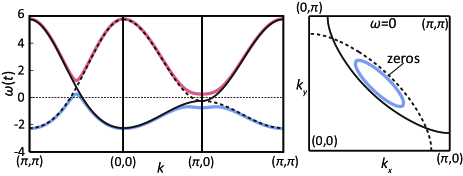
Figure 2: (color online) Left panel shows band dispersions and zero surface along lines running from $(\pi,\pi)$ to $(0,0)$, from $(0,0)$ to $(\pi,0)$, and from $(\pi,0)$ to $(0,0)$. Right panel shows bare and reconstructed Fermi surface, and zero surface at $\omega=0$. Thin (black) solid curve stands for bare band dispersion $\omega=\xi_{k}$, and thin dashed (black) curve stands for zero surface $\omega=\xi_{k+Q_{0}}$. Bold (red and blue) solid curves stand for reconstructed bands.

However, as is already remarked in Sec. I, symmetry breakings such as the antiferromagnetic orders have not been universally observed in the hole-underdoped cuprates where the “Fermi arc” or the truncated Fermi surface has been experimentally suggested. Therefore, we need a mechanism for the emergence of zeros without any symmetry breakings. In this context, the truncated Fermi surface scenario reviewed in Ref.Rice, 2005 gives an interesting example inspired by a result of the renormalization group methods, which attributes the emergence of zeros to Umklapp scatterings without the symmetry breakingsFurukawa et al. (1998). The pseudogap in this framework is the precursor of the Hubbard gap. We employ an alternative framework, where a zero surface with a gap formation naturally emerges by a hybridization with some additional fermionic excitations, as is discussed in the above example of the antiferromagnetic ordered phase, although our additional fermions are different from the quasiparticle at $k+Q_{0}$ in the antiferromagnetic case. Since our pseudogap (the hybridization gap) will turn out to be different from the remnant of the Hubbard gap, our framework will yield results qualitatively different from the scenario by the Umklapp scattering as we see in this paper.

Is there such fermionic excitations in proximity to Mott insulators in the absence of symmetry breakings? Or how do such fermionic excitations emerge? A hint for the existence of such additional fermionic excitations comes from examinations of the LUSW illustrated in Fig. 1 in the doped Mott insulators. Hereafter we restrict our discussion to the hole-doped Mott insulator as in Fig. 1, with the hole-underdoped cuprates in mind. The LUSW is defined as the spectral weight above $\mu$ within the coherent band near the top of the LHB.

We first recall the origin of the LUSW discussed in the literatureMeinders et al. (1993); Phillips et al. (2009). First we begin with the atomic limit, where $t=0$ and $U\neq 0$. Then the LUSW of the hole-doped Mott insulator consists only of states created by adding an $\sigma$-spin electron to an empty site, namely, a holon site, to avoid creating a doubly occupied site, doublon, and to avoid the cost of the on-site Coulomb repulsion $U$. An electron added to an empty site is confined tightly, in this limit. If the electron escapes from the holon sites, it inevitably creates a doublon and costs $U$. In other words, an electron created at a holon site can contribute to the LUSW, although this electron does not propagate coherently.

In the KR formalism, creation (annihilation) operators for the electron at the holon site are given by composite fermion operators $\hat{e}^{\ }_{i}\hat{f}^{\dagger}_{i\sigma}$ ($\hat{f}^{\ }_{i\sigma}\hat{e}^{\dagger}_{i}$). This is just a $\sigma$-spin electron in the original Hubbard model and is definitely fermionic.

When $t/U$ becomes nonzero, we have tightly bound doublons and holons even in the Mott insulating phase. Therefore, holons in the hole-doped systems consist of both of the doped holons and the preexisting holons already present in the insulators. In the hole doped systems, these two types of holons should not be distinguished and should constitute the same object. Then an electron added to these holons should constitute LUSW and may constitute a novel composite particle distinguished from the original electron and offers a hint for the additional fermionic excitations which brings about zeros to the quasiparticle Green’s functions, if this composite particle hybridizes with an original quasiparticle.

Originally the binding energy of a doublon and a holon in the Mott insulator is the order of $U$. However, for finite $t$ and finite doping $x$, indeed, quantum fluctuations induced by coherent carriers dramatically weaken bindings between doublon-holon pairs. Then an electron added to this holon bound to a doublon requires only small energy and merges into the excitation of an added electron to a doped holon site. Actually, remnants of doublon-holon pairs, namely, weakly-bound doublon-holon pairs are known to play an important role in correlated electron systems, especially in the context of variational wave function theoriesKaplan et al. (1982); Yokoyama and Shiba (1990).

A part of the tightly-bound doublon-holon pair, $\overline{e}_{0}\hat{f}^{\dagger}_{i\sigma}$, has already been taken into account in the mean-field level in the previous theories (please note $\hat{e}^{\ }_{i}\hat{f}^{\dagger}_{i\sigma}=\overline{e}_{0}\hat{f}^{\dagger}_{i\sigma}+\widetilde{e}^{\ }_{i}\hat{f}^{\dagger}_{i\sigma}$). However, it represents nothing but the renormalized quasiparticle, which propagates in homogeneous mean fields and has nothing to do with the above composite particle. To substantiate our picture, we need to take into account the composite operator including bosonic fluctuations, $\widetilde{e}^{\ }_{i}\hat{f}^{\dagger}_{i\sigma}$. If we treat such a composite operator $\widetilde{e}^{\ }_{i}\hat{f}^{\dagger}_{i\sigma}$ as a fermion, overlaps between tightly-bound doublon-holon pairs and quasiparticle states cause a hybridization of fermions between two types, where one is the quasiparticle $\hat{f}^{\dagger}_{i\sigma}$ and the other is the “composite fermion” or “cofermion” $\widetilde{e}^{\ }_{i}\hat{f}^{\dagger}_{i\sigma}$. From such a hybridization between the cofermion and quasiparticle, weakly-bound pairs discussed above will naturally be born as a result.

If such a hybridization between the quasiparticle and the composite fermion really exists, this hybridization would contribute to the self-energy of quasiparticles. Depending on the dynamics of the composite fermions, such self-energy would have a strong momentum-dependence and possibly have poles near the zero energy. In such cases, the hybridization between the quasiparticles and the composite particles causes a hybridization gap near the Fermi level. This gap is expected to account for the pseudogap phenomena. As is discussed below, we construct an action containing both of the quasiparticles and the composite fermions.

In the following sections, we concretely give our theoretical treatment by introducing the composite fermions discussed above. First, we list up shortcomings of the previous theories and present our guiding principle to overcome the previous KR’s mean-field theory.

As is mentioned in the above section, the KR formalism gives exact results if we thoroughly take into account the fluctuations of slave bosons and Lagrange multipliers introduced to keep the constraint Eqs.(12) and (13) ( Hereafter we call this constraint the local conservation ). However, the fluctuations of slave bosons are neglected in the original KR’s mean-field theory. In addition, the constraint is also treated just on average. The original constraint is for the operators or the dynamical bosonic fields. In the mean-field theory, the constraint is replaced with averaged density of boson condensations. When we include the fluctuations of slave bosons, we should take care of the constraint or the local conservation of the densities of the slave bosons. In the previous theories, by including the fluctuations of charge bosons, the incoherent Hubbard bands are reproduced. However, there exists a difficulty in conserving spectral weight, because the fluctuations violate the local conservation of the boson densityRaimondi and Castellani (1993).

When we impose the local constraints more strictly for fluctuating bosons beyond the mean-field level, it turns out that the term

$$\hat{\zeta}_{ij\sigma}^{(1)}=g_{1\sigma}^{2}g_{2\sigma}^{2}(\widetilde{p}^{\dagger}_{i\sigma}\widetilde{e}^{\ }_{i}+\widetilde{d}^{\dagger}_{i}\widetilde{p}^{\ }_{i\overline{\sigma}})(\widetilde{e}^{\dagger}_{j}\widetilde{p}^{\ }_{j\sigma}+\widetilde{p}^{\dagger}_{j\overline{\sigma}}\widetilde{d}^{\ }_{j})$$ (65)

represented by the diagram in Fig.3(a) is dominating among all the possible diagrams for the kinetic term in the action Eq. (17), namely

$$\int_{0}^{\beta}d\tau\ \sum_{ij}\hat{f}^{\dagger}_{i\sigma}(\tau)t_{ij}\hat{\zeta}_{ij\sigma}(\tau)\hat{f}^{\ }_{j\sigma}(\tau){.}$$ (66)

Here we employ $g_{1\sigma}^{2}=(1-\overline{p}_{0\overline{\sigma}}^{2}-\overline{e}^{2}_{0})^{-1}$ and $g_{1\sigma}^{2}=(1-\overline{p}_{0\sigma}^{2}-\overline{d}^{2}_{0})^{-1}$ by following Ref.Kotliar and Ruckenstein, 1987.

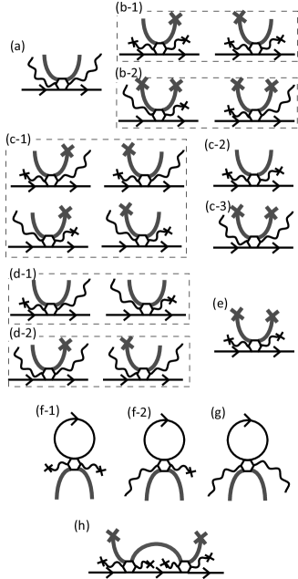
Figure 3: (a)-(e): Diagrams representing terms in $\hat{f}^{\dagger}_{i\sigma}\hat{\zeta}_{ij}\hat{f}^{\ }_{j\sigma}$. (f)-(h): Examples of various diagrams on the one-loop level generated from the coupling (polygons) and derived from the terms (a)-(e). Solid lines with arrows represent propagators of the quasiparticles. Wavy lines stand for the charge bosons, and bold solid lines are the spin bosons. Condensations of bosons are represented by lines terminated at crosses. Coupling constant $g_{1\sigma}^{2}g_{2\sigma}^{2}t_{ij}$ is represented by open polygons. Here, we do not distinguish holons and doublons. Spins are also not distinguished in the diagram, for simplicity.

To elucidate why we retain $\hat{\zeta}_{ij\sigma}^{(1)}$, we classify the diagrams illustrated in Fig.3 into four types, categorized by the time dependence (or frequency dependence) of quasiparticles and the local conservation of the boson densities:

(T-1)

Diagrams containing external propagators of quasiparticles, in addition to bosonic propagators violating the local conservation of boson densities (Figures 3b,3c,3d, and 3h). Here the violation means that before and after the interactions (represented by hexagons), the number of bosons expressed by external boson propagators is not the same.

(T-2)

Diagrams that contain time dependence of quasiparticles, but that do not violate the local conservation (Figures 3a and 3e).

(T-3)

Diagrams that do not contain time dependence of quasiparticles but do violate the local conservation (Fig.3f).

(T-4)

Diagrams that neither include time dependence of quasiparticles nor violate the local conservation (Fig.3g).

Here we present our guiding principle to take account of boson fluctuations: We exclude (T-1) because it violates the local conservation when the quasiparticles dynamically fluctuate. On the other hand we retain diagrams belonging to the categories (T-2), (T-3), and (T-4). The reason to retain these diagram is as follows. The diagrams in the category (T-2) do not violate the local conservation, when bosons fluctuate. Therefore, we take the diagrams in this category into account. On the other hand, the diagrams in the category (T-3) do violate the local conservation. However, in these diagrams, quasiparticles enter as time averaged Green’s functions. Therefore, quasiparticles feel the time averaged bosonic motions. The real violation of the local conservation occurs only when a dynamical quasiparticle process is induced by fluctuating boson hoppings. On the contrary, the real violation does not occur when the quasiparticles emerge as the time averaged quantities as in the case of (T-3). This is the reason to retain the diagrams in the category (T-3). Since (T-4) does not violate local conservation, we retain it.

For the slave-particle formalism of correlated fermion systems, it is wellknown that fluctuations of gauge fields play an important role on reinforcing the local constraint imposed on slave particlesLee et al. (2006). It was pointed out by Jolicoeur and Le Guillou that the Kotliar-Ruckenstein formalism has the $U$(1)$\times$$U$(1)$\times$$U$(1) gauge symmetryJolicoeur and Guillou (1991). It comes from the phase symmetry of the slave bosonic particles, namely, $\hat{e}^{\ }_{i}$, $\hat{p}^{\ }_{i\sigma}$, and $\hat{d}^{\ }_{i}$.

In our theory, we will treat fluctuations of such phases together with fluctuations of the amplitude of the condensation fraction of these slave particles, by using the Bogoliubov prescription. Therefore, the phase fluctuations are taken into account, although the $U$(1)$\times$$U$(1)$\times$$U$(1) gauge structure is not strictly conserved.

III.2 Stratonovich-Hubbard trasformation

We introduce Grassmannian valuables (or fermionic fields) $\hat{\mbox{\boldmath$\Upsilon$}}_{i\sigma}^{\ }=(\hat{\psi}^{\ }_{i\sigma},\hat{\chi}^{\ }_{i\sigma})^{T}$ that stands for the cofermions as are discussed in conceptually in Sec. IIIA. by using the following identity

$$\int\prod_{i\sigma}d\hat{\mbox{\boldmath$\Upsilon$}}_{i\sigma}^{\dagger}d\hat{\mbox{\boldmath$\Upsilon$}}_{i\sigma}^{\ }e^{\mathcal{A}}=\det\left[\widetilde{\mbox{\boldmath$T$}}_{\uparrow}\widetilde{\mbox{\boldmath$T$}}_{\downarrow}\right],$$ (67)

where matrices $\widetilde{\mbox{\boldmath$T$}}_{\sigma}$ are defined as

$$(\widetilde{\mbox{\boldmath$T$}}_{\sigma})_{ij}={g_{1\sigma}^{2}g_{2\sigma}^{2}}{t_{ij}}\left[\begin{array}[]{cc}\widetilde{p}^{\dagger}_{i\sigma}\widetilde{p}^{\ }_{j\sigma}&\widetilde{p}^{\dagger}_{i\sigma}\widetilde{p}^{\dagger}_{j\overline{\sigma}}\\ \widetilde{p}^{\ }_{i\overline{\sigma}}\widetilde{p}^{\ }_{j\sigma}&\widetilde{p}^{\ }_{i\overline{\sigma}}\widetilde{p}^{\dagger}_{j\overline{\sigma}}\end{array}\right],$$ (70)

and

$$\mathcal{A} = \int_{0}^{\beta}d\tau\sum_{ij\sigma}\left[\left(\hat{\mbox{\boldmath$\Upsilon$}}_{i\sigma}^{\dagger}(\tau)-\hat{\mbox{\boldmath$C$}}_{i\sigma}^{\dagger}(\tau)\right)\right.$$ (71)

$$\times \left.(\widetilde{\mbox{\boldmath$T$}}_{\sigma})_{ij}\left(\hat{\mbox{\boldmath$\Upsilon$}}_{j\sigma}^{\ }(\tau)-\hat{\mbox{\boldmath$C$}}_{j\sigma}^{\ }(\tau)\right)\right].$$

Here we use vector notations as

$$\hat{\mbox{\boldmath$C$}}_{i\sigma}^{\dagger} =\left(\widetilde{e}^{\ }_{i},\widetilde{d}^{\dagger}_{i}\right)\hat{f}^{\dagger}_{i\sigma},\ \hat{\mbox{\boldmath$C$}}_{i\sigma}^{\ }=\hat{f}^{\ }_{i\sigma}\left(\widetilde{e}^{\dagger}_{i},\widetilde{d}^{\ }_{i}\right)^{T}.$$ (72)

The identity Eq.(67) gives the transformation for a coupling term of the quasiparticles and fluctuating bosons depicted in Fig.3a,

$$\mathcal{L}_{{\rm a}}=\sum_{ij\sigma}\hat{\mbox{\boldmath$C$}}_{i\sigma}^{\dagger}(\tau)(\widetilde{\mbox{\boldmath$T$}}_{\sigma})_{ij}\hat{\mbox{\boldmath$C$}}_{j\sigma}^{\ }(\tau),$$ (73)

as

$$\exp\left[-\int_{0}^{\beta}d\tau\mathcal{L}_{{\rm a}}\right]=\frac{\displaystyle\int\prod_{i\sigma}d\hat{\mbox{\boldmath$\Upsilon$}}_{i\sigma}^{\dagger}d\hat{\mbox{\boldmath$\Upsilon$}}_{i\sigma}^{\ }e^{-\int_{0}^{\beta}d\tau\mathcal{L^{\prime}}_{a}}}{\det[\widetilde{\mbox{\boldmath$T$}}^{\ }_{\uparrow}\widetilde{\mbox{\boldmath$T$}}^{\ }_{\downarrow}]},$$ (74)

where

$$\mathcal{L^{\prime}}_{a}=\mathcal{L^{\prime}}_{a1}+\mathcal{L^{\prime}}_{a2},$$ (75)

$$\mathcal{L^{\prime}}_{a1}=\sum_{ij\sigma}\hat{\mbox{\boldmath$\Upsilon$}}_{i\sigma}^{\dagger}(\tau)(\widetilde{\mbox{\boldmath$T$}}_{\sigma})_{ij}\hat{\mbox{\boldmath$\Upsilon$}}_{j\sigma}^{\ }(\tau),$$ (76)

$$\mathcal{L^{\prime}}_{a2} = -\sum_{ij\sigma}\left\{\hat{\mbox{\boldmath$C$}}_{i\sigma}^{\dagger}(\tau)(\widetilde{\mbox{\boldmath$T$}}_{\sigma})_{ij}\hat{\mbox{\boldmath$\Upsilon$}}_{j\sigma}^{\ }(\tau)\right.$$ (77)

$$+ \left.\hat{\mbox{\boldmath$\Upsilon$}}_{i\sigma}^{\dagger}(\tau)\widetilde{\mbox{\boldmath$T$}}_{ij}\hat{\mbox{\boldmath$C$}}_{j\sigma}^{\ }(\tau)\right\}.$$

These transformed Lagrangian $\mathcal{L^{\prime}}_{a1}$ (Fig.4a) and $\mathcal{L^{\prime}}_{a2}$ (Fig.4b) lead to the cofermions’ self-energy and the hybridization between the quasiparticles and cofermions, respectively after integrating out the fluctuating bosonic degrees of freedom. It will be discussed below, by using a set of the Dyson equations.

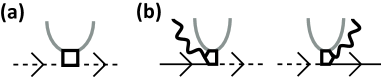
Figure 4: Diagrams for transformed Lagrangians defined in Eqs.(75)-(77). Solid and dashed lines with arrows represent propagators of the quasiparticles and cofermions, respectively. Wavy lines stand for the charge bosons, and bold solid lines are the spin bosons. (a) The diagram represents the Lagrangian $\mathcal{L^{\prime}}_{a1}$ (Eq.(76)). (b) The diagrams stand for terms in the Lagrangian $\mathcal{L^{\prime}}_{a2}$ (Eq.(77)).

III.3 Prescription for self-consistent procedure and Green’s functions

Here we construct approximated Green’s functions for the Gaussian fluctuations of the bosons, quasiparticles, and cofermions by using a set of Dyson equations as is depicted in Fig.5: Wavy lines and bold grey lines stand for the Green’s functions of the charge bosons $\mathcal{A}^{ab}(r,\tau)=-\left\langle T\beta_{i}^{a}(\tau){\beta_{j}^{b}}^{\dagger}(0)\right\rangle,$ and the spin bosons $\mathcal{C}^{ab}(r,\tau)=-\left\langle T\phi_{i}^{a}(\tau){\phi_{j}^{b}}^{\dagger}(0)\right\rangle,$ respectively, where $a,b=1,2$, $r=i-j$, $(\beta_{i}^{1},\beta_{i}^{2})=(\widetilde{e}^{\ }_{i},\widetilde{d}^{\ }_{i})$, and $(\phi_{i}^{1},\phi_{i}^{2})=(\widetilde{p}^{\ }_{i\sigma},\widetilde{p}^{\dagger}_{i\overline{\sigma}})$. Bold lines with arrows represent the quasiparticles propagator $\mathcal{G}_{\sigma}^{(f)}(r,\tau)$. On the other hand, Thin wavy lines and thin lines represent bare propagators of the charge bosons $\mathcal{A}_{0}^{ab}(r,\tau)$, the spin bosons $\mathcal{C}_{0}^{ab}(r,\tau)$, respectively, determined by $\hat{\mathcal{L}}_{{\rm B}}^{(0)}$, in which self-energy effects are not taken into account. Thin lines with arrows stand for bare propagators of the quasiparticles $\mathcal{G}_{0\sigma}^{(f)}(r,\tau)$ determined by

$$\hat{\mathcal{L}}_{0}=\sum_{ij}\hat{f}^{\dagger}_{i\sigma}(\tau)[(\partial_{\tau}-\mu)\delta_{ij}+\zeta_{0\sigma}t_{ij}]\hat{f}^{\ }_{j\sigma}(\tau),$$ (78)

where $\zeta_{0\sigma}=g_{1\sigma}^{2}g_{2\sigma}^{2}(\overline{p}_{0\sigma}\overline{e}_{0}+\overline{d}_{0}\overline{p}_{0\overline{\sigma}})^{2}$. The Lagrangian $\hat{\mathcal{L}}_{0}$ is obtained by decoupling the fluctuating bosons from the KR’s action (see Eq.(17)). Bold and thin dashed lines stand for the cofermions’ propagators $\mathcal{F}^{ab}$ and bare propagators $\mathcal{F}^{ab}_{0}=\delta_{a,b}/\epsilon$ $(\epsilon\rightarrow 0)$, respectively.

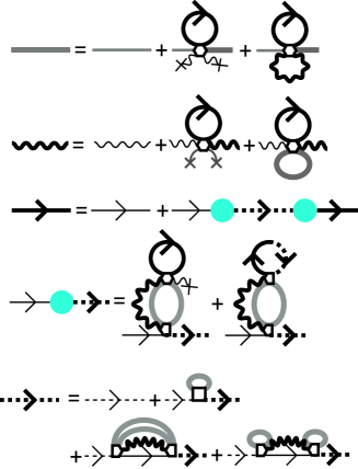
Figure 5: Diagrams for Dyson equations. Solid and dashed lines with arrows represent propagators of the quasiparticles and cofermions, respectively. Other notations are the same as Fig.3. Bold (thin) lines are for renormalized (bare) propagators. Filled (blue) circles are amplitudes of the hybridization between quasiparticles and cofermions.

In the set of Dyson equations (Fig.5), we neglect the coupling between charge and spin bosons described by propagators such as $\left\langle\widetilde{p}^{\dagger}_{i\sigma}\widetilde{e}^{\ }_{i}\right\rangle$, at the Gaussian level, since these coupling terms are higher order contributions. Below we explain that the coupling gives higher order contributions with respect to the hole-doping rate $x$, in proximity to Mott insulating states: Since operators including both charge and spin such as $\widetilde{p}^{\dagger}_{i\sigma}\widetilde{e}^{\ }_{i}$ do not conserve the electric charge, propagators such as $\left\langle\widetilde{p}^{\dagger}_{i\sigma}\widetilde{e}^{\ }_{i}\right\rangle$ should vanish in the Mott insulating phase, where the charge can not fluctuate. Therefore, the charge and spin excitations are well separated in the Mott insulating phase.

When hole carriers are doped, $\widetilde{p}^{\dagger}_{i\sigma}\widetilde{e}^{\ }_{i}$ can have a nonzero expectation value, at most, scaled by the condensate fraction of holons $\overline{e}_{0}$ which gives a rough estimate of the amplitude of charge fluctuations. From a relation $\overline{e}_{0}^{2}\propto x$ held in the KR theory for the hole-doped case, we obtain $\left\langle\widetilde{p}^{\dagger}_{i\sigma}\widetilde{e}^{\ }_{i}\right\rangle\propto\sqrt{x}$. Futhermore, there is an additional constraint for the coupling terms such as $\left\langle\widetilde{p}^{\dagger}_{i\sigma}\widetilde{e}^{\ }_{i}\right\rangle$: they do not appear alone in calculations of physical quantities. To conserve charge and spin on average, $\left\langle\widetilde{p}^{\dagger}_{i\sigma}\widetilde{e}^{\ }_{i}\right\rangle$ appears with $\left\langle\widetilde{e}^{\dagger}_{i}\widetilde{p}^{\ }_{i\sigma}\right\rangle$ in pair, for example. Therefore, the contribution of the coupling between charge and spin bosons to physical quantities is scaled by $(\sqrt{x})^{2}$. It concludes that the coupling between the charge and spin bosons gives contributions as a higher order in terms of $x$ in physical quantities.

By solving the set of Dyson equations, we obtain the propagators for the quasiparticles and cofermions. Here the bosonic degrees of freedom are taken into account in a self-consistent fashion, through the cofermion self-energy $\mbox{\boldmath$\Sigma$}^{({\rm cf})}_{\sigma}(r,\tau)$, and the amplitude $\mbox{\boldmath$\Delta$}_{ij}$ of hybridization between the quasiparticles and cofermions, each of which we detail below.

The Lagrangian for the cofermions is given by

$$\hat{\mathcal{L}}_{{\rm cf}}=-\sum_{ij\sigma}\hat{\mbox{\boldmath$\Upsilon$}}_{i\sigma}^{\dagger}(\tau)\left[\mbox{\boldmath$\Sigma$}^{({\rm cf})}_{\sigma}(r,\tau)\right]\hat{\mbox{\boldmath$\Upsilon$}}_{j\sigma}(\tau),$$ (79)

where $\hat{\mbox{\boldmath$\Upsilon$}}_{i\sigma}^{\dagger}=(\hat{\psi}^{\dagger}_{i\sigma},\hat{\chi}^{\dagger}_{i\sigma})$ is a vector notation for the cofermions, as is defined in the main article, and $r=i-j$. The cofermion self-energy $\mbox{\boldmath$\Sigma$}^{({\rm cf})}_{\sigma}(r,\tau)$ is a 2$\times$2 symmetric matrix,

$$\mbox{\boldmath$\Sigma$}^{({\rm cf})}_{\sigma}=\left[\begin{array}[]{cc}\Sigma_{\sigma}^{11}&\Sigma^{\prime}_{\sigma}\\ \Sigma^{\prime}_{\sigma}&\Sigma_{\sigma}^{22}\\ \end{array}\right].$$ (82)

The details for the self-energy matrix are given in Appendix.A. On the other hand, the hybridization between the quasiparticles and cofermions is described by

$$\hat{\mathcal{L}}_{{\rm hyb}}=\sum_{i,j,\sigma}[\hat{\mbox{\boldmath$\Upsilon$}}_{i\sigma}^{\dagger}(\tau)\mbox{\boldmath$\Delta$}_{ij}\hat{f}^{\ }_{j\sigma}(\tau)+\hat{f}^{\dagger}_{i\sigma}(\tau)\mbox{\boldmath$\Delta$}_{ij}^{T}\hat{\mbox{\boldmath$\Upsilon$}}_{j\sigma}(\tau)],$$ (83)

where $\mbox{\boldmath$\Delta$}_{ij}^{T}=(\Delta_{ij}^{(\psi)},\Delta_{ij}^{(\chi)})$. For details for $\mbox{\boldmath$\Delta$}_{ij}$, see Appendix.B.

As a result, the effective Lagrangian for the quasiparticles and cofermions, $\hat{\mathcal{L}}_{{\rm eff}}$, is given as

$$\hat{\mathcal{L}}_{{\rm eff}}=\hat{\mathcal{L}}_{0}+\hat{\mathcal{L}}_{{\rm cf}}+\hat{\mathcal{L}}_{{\rm hyb}}.$$ (84)

When the charge gap is relatively small, $\Sigma_{\sigma}^{11}\simeq\Sigma_{\sigma}^{22}$ and $\Delta_{ij}^{(\psi)}\simeq\Delta_{ij}^{(\chi)}$ hold approximately. When the charge gap collapses, $\Sigma_{\sigma}^{11}=\Sigma_{\sigma}^{22}$ and $\Delta_{ij}^{(\psi)}=\Delta_{ij}^{(\chi)}$ hold exactly. In our results, we employ approximate relations $\Sigma=\Sigma_{\sigma}^{11}\simeq\Sigma_{\sigma}^{22}$ and $\Delta_{ij}=\Delta_{ij}^{(\psi)}\simeq\Delta_{ij}^{(\chi)}$. Then a cofermion mode $(\hat{\psi}^{\ }_{k\sigma}+\hat{\chi}^{\ }_{k\sigma})/\sqrt{2}$ hybridizes with quasiparticles through the amplitude $\Delta(k)$, which is depicted in Fig.5 as closed (blue) circles, where $k$ is a momentum. The inverse of cofermion propagator (namely, the cofermion self-energy) for $(\hat{\psi}^{\ }_{k\sigma}+\hat{\chi}^{\ }_{k\sigma})/\sqrt{2}$ is given as

$$\frac{-1}{2}[\Sigma_{\sigma}(k,i\varepsilon_{n})+\Sigma^{\prime}_{\sigma}(k,i\varepsilon_{n})]=\gamma_{k}i\varepsilon_{n}-\alpha_{k}+O(\varepsilon_{n}^{2}),$$ (85)

where $\varepsilon_{n}$ is a fermionic Matsubara frequency.

Then, the Green’s function for the quasiparticles is given as

$$\mathcal{G}_{\sigma}^{(f)}(k,i\varepsilon_{n}\rightarrow\omega+i\delta)=G_{\sigma}^{(f)}(k,\omega+i\delta)$$

$$\simeq\displaystyle\left[\omega+i\delta-\zeta_{0\sigma}\epsilon_{k}+\mu-\frac{\Delta(k)^{2}}{\gamma_{k}(\omega+i\delta)-\alpha_{k}}\right]^{-1},$$ (86)

where $\epsilon_{k}$ is the Fourier transformation of $t_{ij}$, and $\mu$ is the chemical potential. Here we note that the weights of the two quasiparticle bands split by the zero surface defined by $\omega=\alpha_{k}/\gamma_{k}$ are not the same in our theory.

In our calculations, we define the doping rate $x$ by using the quasiparticle Green’s function as

$$1-x=\lim_{T\rightarrow 0+}\frac{T}{N_{s}}\sum_{k,i\varepsilon_{n},\sigma}\mathcal{G}_{\sigma}^{(f)}(k,i\varepsilon_{n}),$$ (87)

where $T$ stands for temperature and $N_{s}$ is the number of sites.

The Green’s function for the electrons, instead of the quasiparticles, is given as

$$\mathcal{G}_{ij\sigma}(\tau) = -\left\langle T\hat{c}^{\ }_{i\sigma}(\tau)\hat{c}^{\dagger}_{j\sigma}(0)\right\rangle$$ (88)

$$\simeq -\left\langle T\hat{z}^{\dagger}_{i\sigma}(\tau)\hat{z}^{\ }_{j\sigma}(0)\right\rangle$$

$$\times \left\langle T\hat{f}^{\ }_{i\sigma}(\tau)\hat{f}^{\dagger}_{j\sigma}(0)\right\rangle$$

$$= \left\langle T\hat{z}^{\dagger}_{i\sigma}(\tau)\hat{z}^{\ }_{j\sigma}(0)\right\rangle\mathcal{G}^{(f)}_{ij\sigma}(\tau),$$

where the bosonic and fermionic degrees of freedom are decoupled, because the resultant action in our theory does not contain the hybridization between bosons and fermions. The quasiparticle Green’s function is defined, as in the previous sections, as

$$\mathcal{G}^{(f)}_{ij\sigma}(\tau)=-\left\langle T\hat{f}^{\ }_{i\sigma}(\tau)\hat{f}^{\dagger}_{j\sigma}(0)\right\rangle.$$ (89)

The bosonic part in Eq.(88) is given by

$$\left\langle T\hat{z}^{\dagger}_{i\sigma}(\tau)\hat{z}^{\ }_{j\sigma}(0)\right\rangle \simeq g_{1\sigma}^{2}g_{2\sigma}^{2}\left\langle T[\hat{\mbox{\boldmath$b$}}^{\dagger}_{i}(\tau)\cdot\hat{\mbox{\boldmath$p$}}^{\ }_{i\sigma}(\tau)]\right.$$ (90)

$$\times \left.[\hat{\mbox{\boldmath$p$}}^{\dagger}_{j\sigma}(\tau)\cdot\hat{\mbox{\boldmath$b$}}^{\ }_{j}(\tau)]\right\rangle,$$

where we use vector notation as $\hat{\mbox{\boldmath$b$}}^{\dagger}_{i}=(\hat{e}^{\dagger}_{i},\hat{d}^{\ }_{i})$, $\hat{\mbox{\boldmath$p$}}^{\dagger}_{i\sigma}=(\hat{p}^{\dagger}_{i\sigma},\hat{p}^{\ }_{i\overline{\sigma}})$. Because we adopt the boson dynamics in which charge and spin bosons are decoupled, this bosonic part of the Green’s function is rewritten as

$$\left\langle T\hat{z}^{\dagger}_{i\sigma}(\tau)\hat{z}^{\ }_{j\sigma}(0)\right\rangle$$

$$\simeq g_{1\sigma}^{2}g_{2\sigma}^{2}\left\langle T[\overline{\mbox{\boldmath$b$}}_{0}\cdot\overline{\mbox{\boldmath$p$}}_{0\sigma}^{T}][\overline{\mbox{\boldmath$p$}}_{0\sigma}\cdot\overline{\mbox{\boldmath$b$}}_{0}^{T}]\right\rangle$$

$$+g_{1\sigma}^{2}g_{2\sigma}^{2}\left\langle T[\widetilde{\mbox{\boldmath$b$}}^{\dagger}_{i}(\tau)\cdot\overline{\mbox{\boldmath$p$}}_{0\sigma}^{T}][\overline{\mbox{\boldmath$p$}}_{0\sigma}\cdot\widetilde{\mbox{\boldmath$b$}}^{\ }_{j}(\tau)]\right\rangle$$

$$+g_{1\sigma}^{2}g_{2\sigma}^{2}\left\langle T[\overline{\mbox{\boldmath$b$}}_{0}\cdot\widetilde{\mbox{\boldmath$p$}}^{\ }_{i\sigma}(\tau)][\widetilde{\mbox{\boldmath$p$}}^{\dagger}_{j\sigma}(\tau)\cdot\overline{\mbox{\boldmath$b$}}_{0}^{T}]\right\rangle$$

$$+g_{1\sigma}^{2}g_{2\sigma}^{2}\left\langle T[\widetilde{\mbox{\boldmath$b$}}^{\dagger}_{i}(\tau)\cdot\widetilde{\mbox{\boldmath$p$}}^{\ }_{i\sigma}(\tau)][\widetilde{\mbox{\boldmath$p$}}^{\dagger}_{j\sigma}(\tau)\cdot\widetilde{\mbox{\boldmath$b$}}^{\ }_{j}(\tau)]\right\rangle,$$ (91)

where $\overline{\mbox{\boldmath$b$}}_{0}=(\overline{e}_{0},\overline{d}_{0})$ and $\overline{\mbox{\boldmath$p$}}_{0\sigma}=(\overline{p}_{0\sigma},\overline{p}_{0\overline{\sigma}})$. If we retain only the first and second lines of the right hand side of Eq.(91), the electron Green’s function is reduced to that already obtained in Ref.Raimondi and Castellani, 1993. The contribution of the fourth line in the right hand side of Eq.(91) is small compared with these from other lines in Eq.(91) because it is the fourth order in the terms of the fluctuation denoted by tildes, and we ignore the fourth term.

III.4 Superconductivities mediated by cofermions and charge bosons

In this subsection, we examine how the present insight from the novel cofermion excitations offers the mechanism for the emergence of superconductivity. Here we examine the singlet superconductivity induced by exchanging one charge boson (see Fig.6).

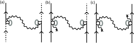
Figure 6: Interactions between quasiparticles and cofermions mediated by exchanging one charge boson.

We start from the mean-field action for the singlet superconductivity. Here the effective interaction of quasiparticles and cofermions is induced by exchanging one charge boson. The mean-field action $S_{{\rm SC}}$ is defined as

$$S_{{\rm SC}}=\sum_{k,i\varepsilon_{n}}\mbox{\boldmath$\Phi$}^{\dagger}_{k}(i\varepsilon_{n})\left[\mbox{\boldmath$\mathcal{G}$}(k,i\varepsilon_{n})\right]^{-1}\mbox{\boldmath$\Phi$}^{\ }_{k}(i\varepsilon_{n}),$$ (92)

where $\mbox{\boldmath$\Phi$}^{\dagger}_{k}(i\varepsilon_{n})$ and $\mbox{\boldmath$\Phi$}^{\ }_{k}(i\varepsilon_{n})$ are defined as

$$\mbox{\boldmath$\Phi$}^{\dagger}_{k}(i\varepsilon_{n}) = \left[\hat{f}^{\dagger}_{k\uparrow}(i\varepsilon_{n}),\hat{\psi}^{\dagger}_{k\uparrow}(i\varepsilon_{n})+\hat{\chi}^{\dagger}_{k\uparrow}(i\varepsilon_{n}),\hat{f}^{\ }_{-k\downarrow}(-i\varepsilon_{n}),\hat{\psi}^{\ }_{-k\downarrow}(-i\varepsilon_{n})+\hat{\chi}^{\ }_{-k\downarrow}(-i\varepsilon_{n})\right],$$ (93)

$$\mbox{\boldmath$\Phi$}^{\ }_{k}(i\varepsilon_{n}) = \left[\hat{f}^{\ }_{k\uparrow}(i\varepsilon_{n}),\hat{\psi}^{\ }_{k\uparrow}(i\varepsilon_{n})+\hat{\chi}^{\ }_{k\uparrow}(i\varepsilon_{n}),\hat{f}^{\dagger}_{-k\downarrow}(-i\varepsilon_{n}),\hat{\psi}^{\dagger}_{-k\downarrow}(-i\varepsilon_{n})+\hat{\chi}^{\dagger}_{-k\downarrow}(-i\varepsilon_{n})\right]^{T}.$$ (94)

The inverse of the matrix form of the Green’s function is given by

$$\left[\mbox{\boldmath$\mathcal{G}$}(k,i\varepsilon_{n})\right]^{-1}=\left[\begin{array}[]{cccc}i\varepsilon_{n}-\xi_{k}&\Delta_{k}&M_{k}&\Lambda_{k}\\ \Delta_{k}&\gamma_{k}i\varepsilon_{n}-\alpha_{k}&\Lambda_{k}&0\\ M_{k}&\Lambda_{k}&i\varepsilon_{n}+\xi_{k}&-\Delta_{k}\\ \Lambda_{k}&0&-\Delta_{k}&\gamma_{k}i\varepsilon_{n}+\alpha_{k}\\ \end{array}\right]$$ (99)

$$=\left[\begin{array}[]{cccc}1&0&0&0\\ 0&\sqrt{\gamma_{k}}&0&0\\ 0&0&1&0\\ 0&0&0&\sqrt{\gamma_{k}}\\ \end{array}\right]\left[\begin{array}[]{cccc}i\varepsilon_{n}-\xi_{k}&\widetilde{\Delta}^{\ }_{k}&M_{k}&\widetilde{\Lambda}^{\ }_{k}\\ \widetilde{\Delta}^{\ }_{k}&i\varepsilon_{n}-\widetilde{\alpha}^{\ }_{k}&\widetilde{\Lambda}^{\ }_{k}&0\\ M_{k}&\widetilde{\Lambda}^{\ }_{k}&i\varepsilon_{n}+\xi_{k}&-\widetilde{\Delta}^{\ }_{k}\\ \widetilde{\Lambda}^{\ }_{k}&0&-\widetilde{\Delta}^{\ }_{k}&i\varepsilon_{n}+\widetilde{\alpha}^{\ }_{k}\\ \end{array}\right]\left[\begin{array}[]{cccc}1&0&0&0\\ 0&\sqrt{\gamma_{k}}&0&0\\ 0&0&1&0\\ 0&0&0&\sqrt{\gamma_{k}}\\ \end{array}\right],$$ (112)

where $\xi_{k}=\zeta_{0}\epsilon_{k}-\mu$, and $M_{k}$ and $\Lambda_{k}$ are superconducting order parameters as is explicitly given in Eqs.(125) and (126). Here the superconducting order parameters are given as

$$M_{k}(i\varepsilon_{n}) = \frac{T}{N_{s}}\sum_{i\omega_{m},Q}\widetilde{t}_{k}\widetilde{t}_{k+Q}\left\langle\widetilde{b}^{\dagger}_{Q}(i\omega_{m})\widetilde{b}^{\ }_{Q}(i\omega_{m})\right\rangle$$ (113)

$$\times \left[\left(\frac{\overline{e}_{0}+\overline{d}_{0}}{\sqrt{2}}\right)^{2}\left[\mbox{\boldmath$\mathcal{G}$}(k+Q,i\varepsilon_{n}+i\omega_{m})\right]_{13}+\frac{\overline{e}_{0}+\overline{d}_{0}}{\sqrt{2}}\left[\mbox{\boldmath$\mathcal{G}$}(k+Q,i\varepsilon_{n}+i\omega_{m})\right]_{14}\right]$$

and

$$\Lambda_{k}(i\varepsilon_{n}) = \frac{T}{N_{s}}\sum_{i\omega_{m},Q}\widetilde{t}_{k}\widetilde{t}_{k+Q}\left\langle\widetilde{b}^{\dagger}_{Q}(i\omega_{m})\widetilde{b}^{\ }_{Q}(i\omega_{m})\right\rangle$$ (114)

$$\times \left[\left[\mbox{\boldmath$\mathcal{G}$}(k+Q,i\varepsilon_{n}+i\omega_{m})\right]_{14}+\frac{\overline{e}_{0}+\overline{d}_{0}}{\sqrt{2}}\left[\mbox{\boldmath$\mathcal{G}$}(k+Q,i\varepsilon_{n}+i\omega_{m})\right]_{13}\right],$$

where $\left[\mbox{\boldmath$\mathcal{G}$}(k+Q,i\varepsilon_{n}\right]_{ij}$ is the ($i,j$)-th element of the matrix $\mathcal{G}$. We should note that there are quasiparticle-quasiparticle and cofermion-quasiparticle singlet pairings, which are described by following anomalous Green’s functions:

$$\left[\mbox{\boldmath$\mathcal{G}$}(k,i\varepsilon_{n})\right]_{13} = \frac{2\widetilde{\alpha}^{\ }_{k}\widetilde{\Delta}^{\ }_{k}\widetilde{\Lambda}^{\ }_{k}-M_{k}\left[\left(i\varepsilon_{n}\right)^{2}-\widetilde{\alpha}_{k}^{2}\right]}{\left[\left(i\varepsilon_{n}\right)^{2}-\lambda_{k+}^{2}\right]\left[\left(i\varepsilon_{n}\right)^{2}-\lambda_{k-}^{2}\right]},$$ (115)

$$\left[\mbox{\boldmath$\mathcal{G}$}(k,i\varepsilon_{n})\right]_{14} = \frac{1}{\sqrt{\gamma_{k}}}\frac{-M_{k}\widetilde{\Delta}^{\ }_{k}\left(i\varepsilon_{n}-\widetilde{\alpha}^{\ }_{k}\right)+\widetilde{\Lambda}^{\ }_{k}\left[\widetilde{\Lambda}_{k}^{2}+\widetilde{\Delta}_{k}^{2}-\left(i\varepsilon_{n}-\widetilde{\alpha}^{\ }_{k}\right)\left(i\varepsilon_{n}+\xi_{k}\right)\right]}{\left[\left(i\varepsilon_{n}\right)^{2}-\lambda_{k+}^{2}\right]\left[\left(i\varepsilon_{n}\right)^{2}-\lambda_{k-}^{2}\right]},$$ (116)

where

$$\lambda_{k\pm} = \frac{\sqrt{X_{k}\pm\sqrt{X_{k}^{2}-4Y_{k}}}}{\sqrt{2}},$$ (117)

$$X_{k} = \widetilde{\alpha}_{k}^{2}+\xi_{k}^{2}+2\widetilde{\Delta}_{k}^{2}+2\widetilde{\Lambda}_{k}^{2}+2M_{k}^{2},$$ (118)

$$Y_{k} = \left(\widetilde{\alpha}_{k}M_{k}+2\widetilde{\Delta}\widetilde{\Lambda}_{k}\right)^{2}+\left[\widetilde{\alpha}_{k}\xi_{k}+\left(\widetilde{\Lambda}_{k}^{2}-\widetilde{\Delta}_{k}^{2}\right)\right]^{2}.$$ (119)

For simplicity, we introduce the cut off frequency

$$\omega_{c}={\rm max}\left\{\zeta_{0}t,\sqrt{\widetilde{\Lambda}_{k}^{2}+M_{k}^{2}}\right\},$$ (120)

to the bosonic propagators for charge fluctuations $\widetilde{b}^{\dagger}_{i}=\widetilde{e}^{\dagger}_{i}+\widetilde{d}^{\ }_{i}$ and apply a quasi-static approximation to solve the gap equations as

$$M_{k}(i\varepsilon_{n}) \times \left[\left(\frac{\overline{e}_{0}+\overline{d}_{0}}{\sqrt{2}}\right)^{2}\left[\mbox{\boldmath$\mathcal{G}$}(k+Q,i\varepsilon_{n}+i\omega_{m})\right]_{13}+\frac{\overline{e}_{0}+\overline{d}_{0}}{\sqrt{2}}\left[\mbox{\boldmath$\mathcal{G}$}(k+Q,i\varepsilon_{n}+i\omega_{m})\right]_{14}\right]$$

$$\simeq \frac{1}{N_{s}}\sum_{Q}\widetilde{t}_{k}\widetilde{t}_{k+Q}\left\langle\widetilde{b}^{\dagger}_{Q}(\omega_{c})\widetilde{b}^{\ }_{Q}(\omega_{c})\right\rangle T\sum_{i\omega_{m}}\left[\left(\frac{\overline{e}_{0}+\overline{d}_{0}}{\sqrt{2}}\right)^{2}\left[\mbox{\boldmath$\mathcal{G}$}(k+Q,i\varepsilon_{n}+i\omega_{m})\right]_{13}\right.$$

$$+ \left.\frac{\overline{e}_{0}+\overline{d}_{0}}{\sqrt{2}}\left[\mbox{\boldmath$\mathcal{G}$}(k+Q,i\varepsilon_{n}+i\omega_{m})\right]_{14}\right]$$ (122)

and

$$\widetilde{\Lambda}_{k}(i\varepsilon_{n}) \times \left[\left[\mbox{\boldmath$\mathcal{G}$}(k+Q,i\varepsilon_{n}+i\omega_{m})\right]_{14}+\frac{\overline{e}_{0}+\overline{d}_{0}}{\sqrt{2}}\left[\mbox{\boldmath$\mathcal{G}$}(k+Q,i\varepsilon_{n}+i\omega_{m})\right]_{13}\right]$$

$$\simeq \frac{1}{\sqrt{\gamma_{k}}}\cdot\frac{1}{N_{s}}\sum_{Q}\widetilde{t}_{k}\widetilde{t}_{k+Q}\left\langle\widetilde{b}^{\dagger}_{Q}(\omega_{c})\widetilde{b}^{\ }_{Q}(\omega_{c})\right\rangle$$

$$\times T\sum_{i\omega_{m}}\left[\left[\mbox{\boldmath$\mathcal{G}$}(k+Q,i\varepsilon_{n}+i\omega_{m})\right]_{14}+\frac{\overline{e}_{0}+\overline{d}_{0}}{\sqrt{2}}\left[\mbox{\boldmath$\mathcal{G}$}(k+Q,i\varepsilon_{n}+i\omega_{m})\right]_{13}\right].$$ (124)

Then we obtain the superconducting states induced with electron-electron and cofermion-electron pairs formed by exchanging one charge boson.

We solve the gap equations Eqs.(122) and (124) with an assumption for the symmetry of the superconducting order parameters. Here we assume a simple $d_{x^{2}-y^{2}}$-symmetry, which has experimentally been suggested for the hole-doped cuprates, for the singlet electron-electron and cofermion-electron pairs as

$$M_{k}(i\varepsilon_{n}) = \frac{M_{d_{x^{2}-y^{2}}}(i\varepsilon_{n})}{2}\left(\cos k_{x}-\cos k_{y}\right),$$ (125)

$$\widetilde{\Lambda}_{k}(i\varepsilon_{n}) = \frac{\widetilde{\Lambda}_{d_{x^{2}-y^{2}}}(i\varepsilon_{n})}{2}\left(\cos k_{x}-\cos k_{y}\right).$$ (126)

As a consequence of the quasi-static approximation, the gap amplitudes $M_{d_{x^{2}-y^{2}}}(i\varepsilon_{n})$ and $\widetilde{\Lambda}_{d_{x^{2}-y^{2}}}(i\varepsilon_{n})$ become constant independently of the Matsubara frequency. Of course, we expect that the amplitudes of $M_{d_{x^{2}-y^{2}}}(i\varepsilon_{n})$ and $\widetilde{\Lambda}_{d_{x^{2}-y^{2}}}(i\varepsilon_{n})$ will damp for $\omega_{{\rm c}}\ll|i\varepsilon_{n}|$.

Here we note how the cofermion-quasiparticle pairs, namely, $\left[\mbox{\boldmath$\mathcal{G}$}\right]_{14}$, enhance the quasiparticle-quasiparticle pairing. First, it is clearly seen in Eq.(113) or (122), that the cofermion-quasiparticle pairs contribute to the superconducting order parameters of the quasiparticle-quasiparticle channel, $M_{k}(i\varepsilon_{n})$. This contribution becomes constructive one, only when the phases of the cofermion-quasiparticle and the quasiparticle-quasiparticle pairs are the same, namely, $M_{k}\cdot\Lambda_{k}>0$. In this case, the interaction illustrated in Fig.6(b) behaves as an attractive interaction between the cofermion-quasiparticle and the quasiparticle-quasiparticle pairs. Then the formation of the cofermion-quasiparticle pairs enhances the quasiparticle-quasiparticle pairing through this attraction, and, indeed, enhances the pairing in our self-consistent solution of Eqs.(122) and (124).

IV Results

In this section, we show how our theory predicts physical properties of our interest. We estimate the quasiparticle and electron Green’s function obtained in the above section, Sec.III.3. We show the results for the Hubbard model defined in Eq.(1) on a square lattice at $U=12t$ and $t^{\prime}=0.25t$ to get insight into the cuprate superconductors. We restrict the mean-field solutions to the homogeneous and paramagnetic ones. All the calculations are done at zero temperature. At this parameter and within the present calculation, the amplitude of the Hubbard gap $\delta U$ at half filling $n=1$ is estimated to be $3.6t$.

First, we give the spectral functions calculated from the electron Green’s function given in Eq.(88), and show the global structure of the spectra obtained from the electron Green’s function. We define the retarded Green’s function at the frequency $\omega$ as

$$G_{\sigma}(k,\omega)=\mathcal{G}_{\sigma}(k,i\varepsilon_{n}\rightarrow\omega+\delta),$$ (127)

where $\delta\rightarrow+0$. Then, the spectral function is given by

$$A(k,\omega)=-\frac{1}{\pi}{\rm Im}\left[G_{\sigma}(k,\omega)\right].$$ (128)

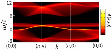
Figure 7: (color online) Spectral function $A(k,\omega)$ along lines running from $(0,0)$ to $(\pi,\pi)$, from $(\pi,\pi)$ to $(\pi,0)$, and from $(\pi,0)$ to $(0,0)$. Here we use a finite broadening factor $\delta=0.05t$.

In Fig.7, we show the result for $x=0.05$. There are two main features. The first is the coherent band seen around the Fermi level, i.e., $\omega=0$. The second is the incoherent spectrum induced by the charge and spin boson dynamics. As is already discussed in Ref.Raimondi and Castellani, 1993, the remnant of the upper Hubbard band is seen above $\omega\simeq 6t$, while the lower Hubbard band is seen between the coherent band and $\omega\simeq-8t$. The gap seen in the spectral function at $2t\lesssim\omega\lesssim 6t$ is nothing but the remnant of the Hubbard gap. Here an additional incoherent band is seen just above the Fermi level up to $\omega\simeq 2t$. This additional incoherent band originates from the dynamics of the spin bosons. The spectral function shown in Fig.7 is qualitatively consistent with the results of the quantum Monte Carlo simulations done by Preuss et al.Preuss et al. (1997), although their simulations were done for $t^{\prime}/t=0$, $U/t=8$ and $T\neq 0$. We note that the dispersion of the coherent band is given by poles of the quasiparticle Green’s function. Below, we concentrate on the low-energy excitations within the coherent band. Therefore, we focus on the quasiparticle Green’s functions instead of electrons Green’s functions.

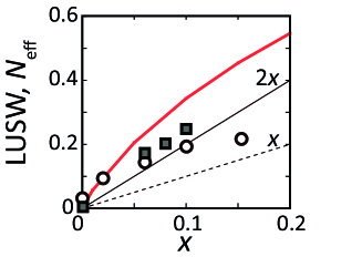
Figure 8: (color online) Bold (red) solid curve shows doping dependence of low-energy spectral weight. Thin (black) solid line represents $2x$ and thin (black) dashed line stand for $x$. Open circles and closed squares illustrate $N_{{\rm eff}}$ given in Ref.Uchida et al., 1991 for La_2-xSr_xCuO₄, and Ref.Waku et al., 2004 for Ca_2-xNa_xCuO₂Cl₂,respectively.

In Fig.8, we show the LUSW defined by $(1+x)\zeta_{0}$ as a function of $x$. The quick increase of the LUSW larger than $2x$ is clearly seen in Fig.8. We refer to the data on the effective electron number $N_{{\rm eff}}$ estimated from the optical conductivity measurementUchida et al. (1991); Waku et al. (2004), which shows nice agreement with the present LUSW at the small doping as is expected. For larger doping the LUSW and $N_{{\rm eff}}$ become trivially different because $N_{{\rm eff}}$ is also proportional to the population of the occupied states and decreases when the number of occupied states becomes small, while the LUSW expresses only the population of unoccupied states and should always be larger than $2x$. LUSW and $N_{{\rm eff}}$ become identical in the small doping asymptotically. The quick increase of LUSW indicates that the Mott gap collapses and interrupted by the quick emergence of the low-energy unoccupied states. This LUSW comes from the quasiparticle band hybridized with the cofermions. The quick increase of the LUSW is also related with a positive feedback of the doping, where the hole doping introduces additional screening of carriers leading to a further increase of unbound holon and doublon. Although the Mott transition is continuous in the low-energy limit at the Fermi level as the ground state properties, this positive feedback gives a character close to the first-order transition in the energy scale of the LUSW, namely in the low-energy excitation spectra. It may be related to the tendency for the phase separation universally suggested in the doped Mott insulators ( including the cuprate superconductors ) which has been discussed from several different viewpointsEmery and Kivelson (1993).

IV.1 Fermi-surface topology

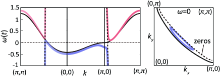
Figure 9: (color online) Left panel shows band dispersions and zero surface calculated for $x=0.05$ along lines running from $(\pi,\pi)$ to $(0,0)$, from $(0,0)$ to $(\pi,0)$, and from $(\pi,0)$ to $(0,0)$. Right panel shows bare and reconstructed Fermi surface, and zero surface at $\omega=0$. Thin solid (black) curve gives the bare band dispersion $\omega=\zeta_{0\sigma}\epsilon_{k}-\mu$, and thin dashed (black) curve represents the zero surface $\gamma_{k}\omega=\alpha_{k}$. Thick (blue and red) solid curves stand for reconstructed bands.

Now we show how the reconstruction of the Fermi surface occurs in our theory. The quasiparticle Green’s function

$$G_{\sigma}^{(f)}(k,\omega)=\mathcal{G}_{\sigma}^{(f)}(k,{i}\varepsilon_{n}\rightarrow\omega+i\delta),$$

is given as

$$G_{\sigma}^{(f)}(k,\omega) = \left[\omega+i\delta-\zeta_{0\sigma}\epsilon_{k}+\mu-\frac{\Delta_{k}^{2}}{\gamma_{k}{\left(\omega+i\delta\right)}-\alpha_{k}}\right]^{-1}$$

$$= \left[\frac{1}{2}+\frac{d^{-}_{k}}{\sqrt{(d^{-}_{k})^{2}+\Delta_{k}^{2}/\gamma_{k}}}\right]\frac{1}{\omega+i\delta-d^{+}_{k}-\sqrt{(d^{-}_{k})^{2}+\Delta_{k}^{2}/\gamma_{k}}}$$

$$+ \left[\frac{1}{2}-\frac{d^{-}_{k}}{\sqrt{(d^{-}_{k})^{2}+\Delta_{k}^{2}/\gamma_{k}}}\right]\frac{1}{\omega+i\delta-d^{+}_{k}+\sqrt{(d^{-}_{k})^{2}+\Delta_{k}^{2}/\gamma_{k}}},$$ (130)

where $d^{\pm}_{k}=\frac{1}{2}\left(\zeta_{0}\epsilon_{k}-\mu\pm\alpha_{k}/\gamma_{k}\right)$. Green’s function given in Eq.(IV.1) shows the divergence of the quasiparticle self-energy given by $\Delta_{k}^{2}/(\gamma_{k}\omega-\alpha_{k})$, at $\gamma_{k}\omega-\alpha_{k}=0$. In other words, the zero surface defined by $\gamma_{k}\omega=\alpha_{k}$ emerges. Then, the zero surface splits the band dispersion defined by $\omega=\zeta_{0\sigma}\epsilon_{k}-\mu$ into two bands as $\omega=d^{+}_{k}\pm\sqrt{(d^{-}_{k})^{2}+\Delta_{k}^{2}/\gamma_{k}}$, as is depicted in Fig.9. For small doping such as $x=0.05$, our theory predicts that the reconstructed Fermi surface becomes a small pocket, as is seen in the right panel of Fig.9.

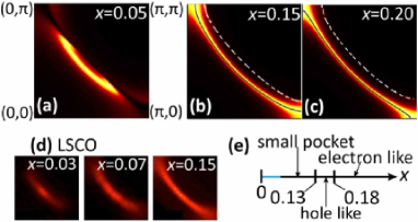
Figure 10: (color online) (a),(b),(c) Single particle spectral function at $\omega=0$. Solid and dashed lines illustrate the poles of quasiparticles. (d) Fermi surface observed by ARPESYoshida et al. (2006). (e) Phase diagram of Fermi-surface topology in our theory. Topological phase boundaries exist at the doping $x=0.13$ and 0.18.

To show changes in the Fermi-surface topology with increasing doping, the single particle spectral function at $\omega=0$ is given for the hole-doping rate, $x=0.05,\ 0.15,\ 0.20$ in Fig.10(a)-(c), with $\delta=0.05t$. The topological transitions occur at $x\simeq 0.13$ and $x\simeq 0.18$, as is depicted in Fig.10(e). In the region $0.13\lesssim x$, only small Fermi pockets exist, where the zero surface smears out the outer part of the pocket yielding an arc structure as we see in Fig.10(a) (note that the damping is large near the zero surface because of an enhanced self-energy), consistently with the experimental signature in Fig. 10(d) as we discuss below. For $0.13\gtrsim x$, a completely different topology with large Fermi surfaces appear, instead of Fermi pockets. For $0.13\lesssim x\lesssim 0.18$, a hole-like surface centered at $(\pi,\pi)$ (depicted by the solid curve in Fig.10(b)) and, an electron-like one centered at $(\pi,\pi)$ (depicted by the dashed curve in Fig.10(b)) coexist. These two surfaces together figure out an enclosed hole (electron unoccupied) strip between the solid and dashed curves. However, the electron-like surface (the dashesd curve) is hardly seen because the zero surface exists near this electron-like surface. On the other hand, for $0.18\gtrsim x$, there exist an electron-like surface centered at $(0,0)$ (depicted by the solid curve in Fig.10(c)), and an electron-like one centered at $(\pi,\pi)$ (depicted by the dashed curve in Fig.10(c)). The electron-like surface centered at $(\pi,\pi)$ becomes less-visible for the used broadening factor $\delta=0.05t$ than the electron-like surface centered at $(\pi,\pi)$ for $x\lesssim 0.18$.

The quantum transition at $x\simeq 0.18$ is a trivial one expected from the single particle picture. The topology of the Fermi surface at this quantum transition point changes from a hole-like surface centered at $(\pi,\pi)$ depicted for $x=0.15$ in Fig.10 by the solid curve, to an electron-like surface centered at $(0,0)$ depicted for $x=0.20$ in Fig.10 by the solid curve. This topology change is essentially understood from the non-interacting picture, where the band dispersion $\epsilon_{k}=-2t(\cos k_{x}+\cos k_{y})+4t^{\prime}\cos k_{x}\cos k_{y}$ with $t^{\prime}/t=0.25$ shows the transition from the electron-like to the hole-like Fermi surfaces with the increasing electron concentrations. When the Fermi level is shifted by doping and touches the saddle points at $(\pm\pi,0)$ and $(0,\pm\pi)$, such topological changes occur.

However, our solution shows another nontrivial topological transition at $x\simeq 0.13$. The topology in the phase $x<0.13$ is highly nontrivial, and is not adiabatically connected with the conventional Fermi liquid. Such a topological change never occurs without the zeros of the Green’s function.

For comparison with experiments, we refer to the ARPES spectrum of La_2-xSr_xCuO₄Yoshida et al. (2006) in Fig.10(d). Arc-like Fermi surfaces observed for $x=0.03$ and $x=0.07$ show overall consistency with our result for $x=0.05$. On the other hand, so-called nodal metallic behaviors, i.e., large amplitude of the spectral weight allowed only around the nodal direction (line running from $(0,0)$ to $(\pi,\pi)$) are not seen in our results. Instead, in our theory, the weight is rather larger near the endpoint of the arc than the nodal point as we see in Fig.10(a). This subtle discrepancy is likely to originate from additional self-energy effects, which are not included in the present theory. For example, fluctuations of $d$-wave superconductivity and/or short range antiferromagnetic fluctuations are possible candidates. However, we note that these fluctuations with finite correlation length by themselves never induce changes in the Fermi-surface topology.

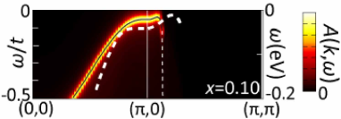
Figure 11: (color online): Single particle spectral function near antinodal point for $x=0.10$. Thin solid and dashed lines illustrate poles of quasiparticles. White bold dashed line stands for ARPES spectrum observed in La_2-xSr_xCuO₄ for $x=0.10$Ino et al. (2002).

When the large Fermi surface appears for $x\gtrsim 0.13$, the Fermi surface always extends across the Brillouin zone boundary or the lines which connect the $\Gamma$ point, $(0,0)$, and the antinodal points $(\pm\pi,0)$ or $(0,\pm\pi)$. However, the single-particle excitation from the Fermi level now has a gap due to the hybridization gap $\Delta_{k}$ in (IV.1) in the quantum phase characterized by the nontrivial Fermi surface topology for $x\lesssim 0.13$. In Fig.11, the single particle spectral function is depicted along the symmetry lines in the Brillouin zone. A gap measured from the Fermi level emerges, which corresponds to the pseudogap in the ARPES measurements. Hereafter, we define the amplitude of the pseudogap in the single particle spectrum, $\Delta$, as the gap amplitude between the Fermi level $\mu$ and the maximum of the single particle dispersion below $\mu$ along the line running from $(0,0)$ to $(\pi,0)$ and the line running from $(\pi,0)$ to $(\pi,\pi)$. We also reproduce the ARPES dispersion observed in La_2-xSr_xCuO₄ for $x=0.10$ Ino et al. (2002) for comparison in Fig.11 (indicated by bold dashed curve). Here we employ a widely accepted parameter $t=$400 meV. Indeed the dispersion has an excellent similarity. The quasiparticle dispersion does not touch the Fermi level along the Brillouin zone boundary, here the line connecting $(\pi,0)$ and $(\pi,\pi)$, in both of our result and the ARPES measurement. In other words, the pseudogap amplitude $\Delta$ is finite for both cases. However, the quasiparticle state at $(\pi,0)$ in the ARPES data has lower energy than our result and the discrepancy is up to 20 meV. We expect some additional factors to push the dispersion down around the antinodal points $(\pm\pi,0)$ and $(0,\pm\pi)$. As is discussed above, fluctuations of $d$-wave superconductivity and/or short range antiferromagnetic fluctuations are possible candidates of the origin of this discrepancy.

IV.2 Pseudogap

The pseudogap in single particle excitations defined in the above section characterizes a quantum phase with the nontrivial Fermi surface, because a nonzero pseudogap induces the breakdown of the trivial large Fermi surface. In our theory, the pseudogap is induced by the hybridization gap between the cofermions and quasiparticles. Therefore, the amplitude of the pseudogap is roughly determined by the hybridization gap $\Delta_{k}/\sqrt{\gamma_{k}}$. The explicit evaluation of the amplitude of $\Delta_{k}$ is done by using Eq.(173) in Appendix.B, in the lowest order of $t_{ij}$. The amplitude of $\Delta_{k}$ is roughly estimated as $t^{2}/W$ multiplied by a numerical factor, where $W$ is the band width of original electrons. Here we note that the denominators in Eq.(173) include the dispersion of the charge and spin bosons. The band width of the charge and spin bosons are roughly equal to the band width of original electrons, $W\simeq 8t$, and the band width of the spin wave, $J\sim 4t^{2}/U$, respectively. For $U=12t$, the band width of the charge bosons dominates that of the spin bonosons, namely, $W>J$. Therefore, the denominators appearing in Eq.(173) are roughly scaled by $W$. On the other hand, the amplitude of $\gamma_{k}$ is roughly estimated as $t^{2}/W^{2}$ multiplied by a numerical factor, through Eq.(170). Therefore, the amplitude of the hybridization gap $\Delta_{k}/\sqrt{\gamma_{k}}$ is roughly estimated as $(t^{2}/W)/\sqrt{t^{2}/W^{2}}=t$ multiplied by a numerical factor. The present result for the energy scale of the pseudogap is consistent with previous studies based on the cluster perturbation theoryS${\rm\acute{e}}$n${\rm\acute{e}}$chal and Tremblay (2004) and, later, cellular DMFTKyung et al. (2006).

We discussed the pseudogap $\Delta$ along the definition often used in ARPES measurements, in IV.1. Here we discuss the behaviors of the hybridization gap between two bands given in Eq.(130) and illustrate in Fig.9. First, the hybridization gap $\Delta_{k}/\gamma_{k}$ in our theory does not have nodes, and is $s$-wave-like in the momentum space, although, as is illustrated in Fig.12, the gap seems to be smaller in the nodal direction (the line running from $(0,0)$ to $(\pi,\pi)$) than around the antinodal points $(\pm\pi,0)$ and $(0,\pm\pi)$.

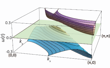
Figure 12: Band dispersion of quasiparticles for $x=0.05$. A full gap structure is clear.

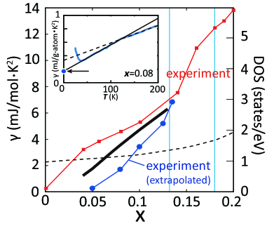
Figure 13: Density of states (DOS) of electrons given as a function of hole doping rate $x$. The thin dashed curve stands for the DOS of the noninteracting case. Closed (blue) circles show $\gamma$ extrapolated from experimental data of La_2-xSr_xCuO₄ in Ref.Loram et al., 2001. Closed (red) squares stand for experimental data of La_2-xSr_xCuO₄ in Ref.Momono et al., 1994. Inset shows an example for extrapolation used here, see the text below Eq.(131) for details.

Below the transition point $x\simeq 0.13$, the density of states (DOS) of the original electrons $\hat{c}^{\dagger}_{k\sigma}$ at the Fermi level, $\rho_{{\rm F}}$, defined as

$$\rho_{{\rm F}}=\zeta_{0}\frac{1}{N_{s}}\sum_{k\sigma}\left[-\frac{1}{\pi}{\rm Im}G_{f\sigma}(k,\omega=0)\right],$$ (131)

is clearly suppressed, as is illustrated in Fig.13. We compare $\rho_{{\rm F}}$ with the specific heat measured for La_2-xSr_xCuO₄Momono et al. (1994); Loram et al. (2001). The specific heat coefficient $\gamma$ is expected to be proportional to the DOS. In the Sommerfeld’s free electron model, the specific heat coefficient $\gamma$ at $T=0$ is given by $\gamma=\pi^{2}\rho_{F}/3.$ Here we use this relation and $t=$400 meV to calculate the expected values for $\gamma$ with our theory.

We note that $\gamma$ in Fig.13 indicated by closed (blue) circles is obtained through a linear extrapolation from low-temperature data in Ref.Loram et al., 2001, and shows the possible lower limit for $\gamma$. From the data in Ref.Loram et al., 2001, $\gamma$ in the underdoped region shows three characteristic temperature ranges. For example, the data for $x=0.08$ (see the inset of Fig.13) show (1) for 100 K$\lesssim T\lesssim 200$ K, a linear-temperature dependence, (2) for 50 K $\lesssim T\lesssim 100$ K, another linear-temperature dependence but with different slope from (1), and (3) for $T\lesssim 50$ K, the BCS-like jump. We linearly extrapolate $\gamma$ for 50 K $\lesssim T\lesssim 100$ K and obtain $\gamma$ at $T=0$. On the other hand, data for $\gamma$ indicated by closed (red) squaresMomono et al. (1994) in Fig.13 may set an upper limit for $\gamma$, because, to exclude the influences from superconductivities, the authors of Ref.Momono et al., 1994 used extrapolation from Zn-doped samples, which tend to show larger $\gamma$ than samples without Zn-doping.

Our result for $\gamma$ is consistent with the experiments, although we do not choose parameters specific to La_2-xSr_xCuO₄. On the other hand, the extrapolated $\gamma$ (closed (blue) circles in Fig.13) indicates further reduction of the density of states at the Fermi level. It suggests possible roles of fluctuations from the $d$-wave superconductivity and/or antiferromagnetism in lower energy scale, which is left for future studies beyond the scope of this paper.

IV.3 Superconductivities

In studies on high-$T_{\rm c}$ superconducting cuprates, the mechanism of the superconductivity is of course the central issue Norman et al. (2005). However, the consensus on the mechanism has not been reached after more than twenty years of the discovery. Here we show how the novel cofermion mechanism for superconductivities developed in Sec. IIID works and reproduces experimental observations on the high-$T_{\rm c}$ superconducting cuprates.

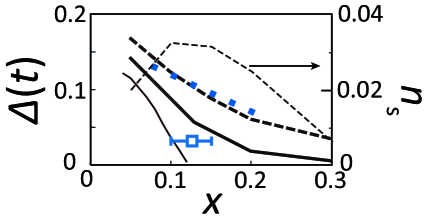
Figure 14: Doping dependence of excitation gaps. The thin (black) solid line stands the pseudogap amplitude in the normal state. This amplitude shows the contribution that has nothing to do with the superconductivity but rather to do with the precursor of the Mott gap. The bold (black) dashed line stands the minimum of the single particle excitation gap in the superconducting state along the Brillouin zone boundary or the diagonal line connecting the $\Gamma$ point and the antinodal points. The bold (black) solid line shows a refined estimate of the single particle excitation gap in the superconducting state obtained from the pair potential mediated by exchanging one charge boson, where the potential is multiplied by a scale factor $\left(1-\zeta_{0}\right)$. The $x$-dependence of excitation gaps observed by ARPES for Bi₂Sr₂CaCu₂O_8+δDing et al. (2001) are indicated by the thick (blue) dotted line. The open square stands for the superconducting gap of optimally doped La_2-xSr_xCuO₄ estimated by ARPES measurementsIno et al. (1999). The thin (black) dashed curve stands for the density of superconducting electrons $n_{{\rm s}}$.

We examine the doping dependence of the single particle excitation gap in the superconducting state based on the formalism developed in Sec. IIID. The result is shown in Fig.14 (bold dashed line). We adopt, as a definition of the amplitude of the gap in the superconducting state, the minimum of the single particle excitation gap along the Brillouin zone boundary and the line connecting the $\Gamma$ point (0,0) and the antinodal points $(\pm\pi,0)$ and $(0,\pm\pi)$, which is the same definition for the pseudogap in the normal state. This definition of the amplitude of the gap is consistent with the data-analysis of the ARPES measurements. As is shown in Fig.14 (bold dashed line), the single particle excitation gap is still finite around $x=0.3$ for the $d$-wave superconducting state in the present treatment, which is quantitatively inconsistent with the experimental fact that the superconductivity disappears for $x\gtrsim 0.26$ in the high-$T_{{\rm c}}$ cuprates. To highlight a possible origin of this inconsistency, we also show a result for the single particle excitation gap in Fig.14 (thick solid line) calculated by rescaling the quasi-static boson propagator as

$$\left\langle\widetilde{b}^{\dagger}_{Q}(\omega_{c})\widetilde{b}^{\ }_{Q}(\omega_{c})\right\rangle\rightarrow\left(1-\zeta_{0}\right)\left\langle\widetilde{b}^{\dagger}_{Q}(\omega_{c})\widetilde{b}^{\ }_{Q}(\omega_{c})\right\rangle.$$

By the rescaling, the single particle excitation gap is clearly suppressed around $x=0.3$. The reason why we consider such a rescaling is the following: In our treatment, the charge fluctuations, especially holon fluctuations remain finite even in the dilute limit $x\rightarrow 1$, where holons fill all the sites and should be localized as hard core bosons. Holons are completely localized and form the “Mott insulating” state for $x=1$. The fluidity of the holons for $x\lesssim 1$ originates from finite electron density, $1-x\neq 0$, because the finite electron density introduces “vacancies” in the holon’s Mott insulating state, and causes the fluidity of the holons. On the other hand, doublons vanish at the limit $x\rightarrow 1$. Near this limit, the density of the doublons are scaled by $(1-x)^{2}$. Therefore, for large doping $x$, the weight of fluctuating charge bosons should vanish as a function of $1-x$. We note that, for $x\simeq 1$, $1-\zeta_{0}\simeq 1-x$. On the other hand, for $x\simeq 0$, the charge fluctuating bosons have the weight $1-\zeta_{0}$, because the incoherent band induced by fluctuating bosons share the total spectral weight with the coherent band, which has the weight $\zeta_{0}$. Therefore for all the doping range, the rescaling of the boson propagators is naturally interpolated by $1-\zeta_{0}$.

Then we compare our result with experimentally observed gap $\Delta$. The result of $\Delta$ without rescaling of the propagators given by the thick dashed curve in Fig.14 shows a rough qualitative agreement with the ARPES result obtained from the single particle excitation gap at low temperatures ($T$=14 K) for Bi₂Sr₂CaCu₂O_8+δDing et al. (2001) (dotted (blue) line in Fig.14). However, our result without the rescaling overestimates $\Delta$ around $x=0.3$, where the superconducting phase is not observed in any of the cuprates. On the other hand, the single particle excitation gap calculated by using the rescaled boson propagator shows a suppression of $\Delta$ around $x=0.3$. The single particle excitation gap $\Delta$ for $x\sim 0.1$ is consistent with the superconducting gap of optimally doped La_2-xSr_xCuO₄ estimated by ARPES measurementsIno et al. (1999) (open square in Fig.14). On the other hand, the rescaled boson propagator appears to be still overestimated for the overdoped region, $x\sim 0.3$. The origin of such overestimated fluctuating charge bosons in our theory may be ascribed to the approximation on the bosonic propagators given in the Dyson equations shown in Fig.5: Lifetime of the coherent propagation of the fluctuating charge bosons is not taken into account in our theory. There exist two possible origins of the finite lifetime. The first is damping caused by single particle excitations, namely, the Landau damping. When the doping increases, the motion of the coherent carriers may disturb the propagation of the fluctuating charge bosons seriously. The second is the separation of charge and spin fluctuations, which becomes a good approximation for $x\simeq 0$. Such separation of charge and spin fluctuations may become worse for large $x$, because the motion of the coherent carriers mixes the charge and spin modes. The mixing of charge and spin fluctuations also disturb the propagation of the fluctuating charge bosons and give a finite lifetime. Therefore, these factors neglected in our theory will suppress the charge fluctuations and consequently, the superconductivities.

The single particle gap $\Delta$ decreases monotonically, as the doping $x$ increases. It is consistent with ARPES measurements. On the other hand, the critical temperature of the superconductivity, $T_{{\rm c}}$, shows a peak around the $x\sim 0.15$ in La_2-xSr_xCuO₄, and exhibits a dome-like structure as a function of $x$. To estimate the tendency of $T_{{\rm c}}$ from our results for $T=0$, we show the $x$-dependences of the density of superconducting electrons $n_{{\rm s}}$ in Fig.14(thin dashed curve) defined as

$$n_{{\rm s}}=\left|\zeta_{0}\frac{T}{N_{{\rm s}}}\sum_{k,i\varepsilon_{n}}\left(\cos k_{x}-\cos k_{y}\right)\left[\mbox{\boldmath$\mathcal{G}$}(k,i\varepsilon_{n})\right]_{13}\right|.$$ (132)

The pairing mechanism proposed here includes the contribution of the cofermion-quasiparticle pairs in addition to the quasiparticle-quasiparticle pairs. This contribution of the cofermion-quasiparticle pairs itself is a novel perspective introduced in this paper. Furthermore, it offers an insight into one of the most interesting issues in physics of the cuprate superconductors, namely, relationship between the pseudogap formation and the high-$T_{{\rm c}}$ superconductivity. The cofermions induce the hybridization gap around the Fermi level, and as a result, the pseudogap. The pseudogap formation itself reduces the DOS around the Fermi level and is harmful for the high-$T_{{\rm c}}$ superconductivity. However, the cofermions support the high-$T_{{\rm c}}$ superconductivity through the cofermion-quasiparticle pairing, simultaneously. Therefore the pseudogap structure does not necessarily destroy the superconducting pairing. The pseudogap formation is the other side of the coin of the cofermion pairing contributing to the superconductivity. This dual character offers an in sight into the recent controversy called dichotomy observed in ARPES measurements Tanaka et al. (2006); Yang et al. (2008): There exist two major pictures for the relationship between the pseudogap and high-$T_{{\rm c}}$ superconductivity. One tells us that the pseudogap is a precursor of the Mott gapFurukawa et al. (1998), and coexists with the superconducting gap. The other claims that preformed pairs of strong coupling superconductivities induce the pseudogapYanase et al. (2003). The present theory offers a new alternate route of understanding that reconciles the dichotomy.

By exchanging one charge boson, attractive interactions are induced for forward scattering channels. Even though there is the strong on-site repulsion $U$, such attractive interactions may favor anisotropic superconductivities not only the $d_{x^{2}-y^{2}}$-wave superconductivity but also, for example, $d_{xy}$-wave and extended $s$-wave superconductivities. In the present theory, however, a simple extended $s$-wave superconducting parameter proportional to $\cos k_{x}+\cos k_{y}$ does not develop.

IV.4 Metal-insulator transitions

We propose a scenario for the filling control metal-Mott insulator transitions based on our theory. Before going into our scenario, we note that there is a difficulty in our theory in the small doping limit $x\rightarrow+0$. In this limit, we have Fermi pockets with small but finite volume depending on parameters such as $t^{\prime}/t$ and $U/t$. It is in contrast to the zero-doping limit of the ordered insulators. In our theory, the weights of the two bands split by the zero surface illustrated in Fig.9 are not the same. From Eq.(130), these weights are given as

$$\frac{1}{N_{{\rm s}}}\sum_{k}\left[\frac{1}{2}\pm\frac{d^{-}_{k}}{\sqrt{(d^{-}_{k})^{2}+\Delta_{k}^{2}/\gamma_{k}}}\right].$$ (133)

In the case of the antiferromagnetic ordered state, the counterparts of these weights are given by

$$\frac{1}{N_{{\rm s}}}\sum_{k}\left[\frac{1}{2}\pm\frac{\epsilon_{1k}}{2\sqrt{\epsilon_{1k}^{2}+\Delta_{{\rm AFM}}^{2}}}\right],$$ (134)

from Eq.(64), and are the same, because of

$$\frac{1}{N_{{\rm s}}}\sum_{k}\frac{\epsilon_{1k}}{2\sqrt{\epsilon_{1k}^{2}+\Delta_{{\rm AFM}}^{2}}}=0.$$ (135)

The weight compensation between these two bands split by the zero surface is needed to reproduce ordered insulating phases. On the other hand, our theory does not offer this weight compensation. Therefore, our theory does not necessarily predict that the small hole pockets seen in Fig.10(a) shrink to points at the small doping limit $x\rightarrow+0$.

In addition, in the limit $x\rightarrow+0$, the imaginary part of the quasiparticle and cofermion self-energy, which is not taken into account in the present theory, may affect the weight compensation. Higher order corrections to the cofermion dynamics will also affect the structure of the zero surface in this limit.

Despite these limitations, our result still suggest a possible scenario for the filling control metal-Mott insulator transitions. If the small Fermi pockets seen in Fig.10(a) shrink to the Fermi points, the filling control metal-insulator transition occurs as a topological transition. On the other hand, if the small Fermi pockets do not shrink to the Fermi points, the quasiparticle weight of the Fermi pockets becomes zero, in spite of the finite volume of pockets. Then the insulating state appears, because of the fading out of the coherent band. In both of the two cases, a small but finite DOS is expected in the limit $x\rightarrow+0$. It should be noted that, anyway, a nontrivial topological transition is expected to occur at a finite doping, before the system becomes insulating.

Here we note that the order of the three quantum phase transitions, namely, the Mott transition at $x=0$, and the two topological transitions at $x\sim 0.13$ and $x\sim 0.18$ are all continuous within the present calculated results, although in general, the first order transition is not a priori excluded. If a topological quantum phase transition takes place as a continuous one at $T=0$, it becomes just a crossover at nonzero temperature, because the Fermi surface is in the strict sense not well defined at $T>0$ and the toplogical character of the Fermi surface loses well-defined meaning at $T>0$ any more. It has been stressed before that the sharp change between the overdoped and underdoped regions is associated with some kind of quantum criticality triggered by a quantum phase transition of the symmetry breaking order. In this conventional quantum criticality, the phase transition usually extends to nonzero temperature as the border of symmetry broken phase. However, the present quantum criticality is completely different from this category, where not the symmetry breaking but the topology change drives the transitionImada (2005); Misawa et al. (2006); Yamaji et al. (2006); Misawa and Imada (2007).

V Summary and Discussions

In this paper, we have proposed a microscopic mechanism for the Fermi-surface reconstruction and non-Fermi-liquid behaviors emerging in proximity to the Mott insulators, motivated by puzzles experimentally observed in the underdoped cuprates. We construct our theory starting from one of the simplest theory for correlated metals, namely, the slave-boson mean-field theory for the Hubbard model by Kotliar and Ruckenstein (KR). Then a special emphasis is placed on the role of extra charge dynamics on low-energy spectra. We find that hidden cofermionic particles constructed from composite fermions play a crucial role in addition to the quasiparticles described by the previous KR theory. The additional cofermions called holo-electrons and doublo-holes represent substantial low-energy part of the charge dynamics.

Thus introduced new cofermions hybridize with the quasiparticles and cause a hybridization gap represented by zeros of the quasiparticle Green functions. As a result, although the explicit symmetry breaking is absent, the gap identified as the pseudogap of the cuprates naturally comes out. Although the origin of the gap has an apparent similarity to the case of the symmetry-broken phases such as commensurate antiferromagnetic metals, in the sense that both of them can be ascribed to a hybridization gap, the mechanism of the hybridization and the partner of the hybridization are very different from the simple symmetry breaking. The origin of the gap is also different from the Mott gap itself. The large Mott gap in the insulating phase is quickly replaced with the present much smaller hybridization gap upon doping, because the LUSW above the hybridization gap emerges. In the result of the cellular dynamical mean-field theorySakai et al. (2009), this hybridization gap coexists with the clear remnant of Mott gap structure in a much larger energy scale. This indicates that the two gaps are separated phenomena. Thus the pseudogap or the hybridization gap in the underdoped region is not really the precursor of the Mott gap.

When the cofermion strongly hybridizes with the quasiparticles and the resultant hybridization gap splits the quasiparticle band around the Fermi level, Fermi-surface reconstruction occurs in a natural way. The hybridization gap indeed leads to a break-up of the Fermi surface into small hole pockets around the nodal direction, and a phase topologically different from the prediction of the weak coupling picture emerges. This phase realized in the underdoped region is separated by a topological phase transition from the normal Fermi liquid phase in the overdoped region. Our result clearly shows that an unconventional non-Fermi liquid phase emerges in the underdoped region. Such topological changes and an emergence of a new phase are consistent with experimentally observed “Fermi-arc” formation in hole-underdoped cuprates.

The topological quantum phase transition between the conventional Fermi liquid and the non Fermi liquid is a continuous one at $T=0$ within the present approximation. This implies that it transforms to a crossover at nonzero temperature, because the continuous topological transition is well defined only at zero temperature. In principle, it does not exclude a possibility of the first order transition of the topological change, which extends to nonzero temperatures with the critical end point at a nonzero temperatureYamaji et al. (2006). The present results do not support the existence of such a first order transition in agreement with the absence of the clear indication of the first order transition in the experiments.

Our formulation offers a new concept for the “pseudogap” phenomena observed in hole-underdoped cuprates. It proposes that the “pseudogap” in the single particle spectrum results from the hybridization gap between the cofermions and the quasiparticles. The part below the Fermi level has the maximum in the antinodal region and has a structure similar to the $d_{x^{2}-y^{2}}$ symmetry in agreement with the experimental observation. The main part of the gap lies, however, above the Fermi level. The total hybridization gap has the structure of the $s$-wave gap.

Consequently, the characteristic energy scale of the pseudogap is identified as that of the hybridization gap amplitude and thus basically scaled by the bandwidth (kineic energy) of the bare electrons, $t$ multiplied by a numerical factor. Therefore, the energy scale of the “pseudogap” has something to do neither with the Hubbard gap or the on-site Coulomb repulsion $U$ nor with the superexchange interaction $J\sim t^{2}/U$.

We have also numerically studied the relevance of our theory in the realistic condition. For the on-site Coulomb repulsion $U$ large enough to create the Hubbard gap $U\gtrsim 10t$ and small amount of hole doping $x\lesssim 0.1$, regarded as a relevant parameter for the high-$T_{c}$ cuprates, the structure of the momentum dependence and the amplitude of the pseudogap below the Fermi level have a quantitative consistency between the ARPES measurements for the hole-doped cuprates and the present results. Doping dependence of the pseudogap amplitude is also consistent with the experimental observation.

Reduction of the electronic density of states induced by the pseudogap formation gives another consistency with the experiments as observed as specific heat coefficients. The pseudogap formation in our theory also induces asymmetry of the DOS around the Fermi level, which naturally explains the asymmetric STM spectraRenner et al. (1998); Hanaguri et al. (2004). The overall consistency supports that the cofermions, holo-electrons and dublo-holes, are indeed a relevant object to be considered in physics of the cuprate superconductors.

The present theory has further consequences and predictions for experiments. The hybridization gap basically has a $s$-wave-like symmetry and a major part of the gap lies above the Fermi level for the model of the hole doped cuprates. Although the present resolution limit of the inverse photoemission does not allow determination of the detailed structure of the unoccupied electronic states, we propose that our prediction of this $s$-wave-like gap structure accompanied by the main part of the LUSW lying above the hybridization gap can be tested experimentally if some high-resolution measurements of the unoccupied spectra are provided. The optical conductivity $\sigma(\omega)$, especcially mid-infrared peak and a long tail of $\sigma(\omega)$ observed in the underdoped cuprates indeed supports the existence of such LUSWUchida et al. (1991); Waku et al. (2004).

So far, direct measurement of the cofermions appears to be difficult, because the dispersion of the cofermions corresponds to the zeros of the quasiparticles, while the zeros are in general hard to detect. In addition, the cofermion does not have a charge and does not allow an electromagnetic detection. However, it contributes to the entropy and thermal transport. Since the electric conduction is contributed only from the quasiparticle, while the thermal transport can arise from the cofermion as well, we expect a serious breakdown of the Wiedeman-Franz (WF) law. The WF law predicts that the ratio of the thermal conductivity $\kappa$ to the electric conductivity $\sigma$ is equal to $L_{0}T$, namely, $L_{0}=\kappa/T\sigma$, where $L_{0}$ is a universal constant given by $L_{0}=(\pi^{2}/3)\cdot\left(k_{{\rm B}}/e\right)^{2}$, namely, the Lorenz number. On the other hand, in our theory, the ratio $L=\kappa/T\sigma$ is predicted to be larger than $L_{0}$ in proximity to Mott insulators, because the cofermions carry additional energy, and contribute to $\kappa$. Indeed the breakdown of the Wiedeman-Franz law reported recently in hole-underdoped cupratesProust et al. (2005) supports the present prediction.

We propose a scenario for the filling control metal-Mott insulator transitions in two dimensions based on the newly introduced cofermions. We predict a pseudogap formation and consequently a non-trivial change in the Fermi-surface topology in the underdoped region. Then the criticality of the small Fermi pockets determines the nature of the Mott transition, if the transition is continuous. Two scenarios remain possible: On the verge of the Mott transition, it may either shrink to points before vanishing by keeping the quasiparticle weight nonzero, or the quasiparticle weight decreases to vanish by keeping a finite volume of the Fermi surface. In the former case, the filling control metal-Mott insulator transitions occur as a topological one. The density of states remain nonzero and finite on the verge of the transition because of the two deminsionality. In the latter case, the effective mass diverges. These two possibilities are essentially identical to the two types discussed in the literatureImada (1993). Although the present numerical accuracy is not sufficient for determining the ultimate criticality, the shrinkage of the pocket and arc overall supports the former scenario, while the reduction of the DOS suggests only a part of the pocket contributes to low-energy excitations as the arc. This agrees with the experimental results. More detailed and accurate determination of the criticality is left for future studies.

We also propose a novel mechanism for high-temperature superconductivity driven by the cofermion-quasiparticle pairing. It offers a new insight into the relationship between the pseudogap formation and the high-$T_{{\rm c}}$ superconductivity. The cofermions newly introduced in the present paper induce the hybridization gap around the Fermi level, and as a result, the pseudogap. This pseudogap formation itself reduces the DOS around the Fermi level and destroys superconductivity. On the other hand, the cofermions enhance the high-$T_{{\rm c}}$ superconductivity through the cofermion-quasiparticle pairing, simultaneously. At the present level of approximation, in the overdoped region, a process exchanging one charge boson overestimates the charge fluctuations and predicts much larger single particle gap in superconducting phases, than experimentally observed gaps. It is left for future studies to correct such an overestimate of charge fluctuations. In addition to one charge boson exchange processes, cofermion polarization will help the pairing between quasiparticles, which is not taken into account as a higher order contribution in the present paper. However, the superconducting gap obtained from the present approximation already reproduces the dome-like structure as a function of the doping concentration with a right order of magnitude if we compare with the cuprates.

Although we focus on the hole-doped cuprates in this paper, electron-underdoped cuprates are also interesting from the viewpoint of the present cofermion theory. In the electron-underdoped systems, our theory will predict the emergence of two electron pockets centered at $(\pi,0)$ and $(0,\pi)$ even in the absence of antiferromagnetic long-range orders. Such a Fermi-surface topology may reduce instabilities towards antiferromagnetic orders, and will make $d_{x^{2}-y^{2}}$-wave superconductivities stable: The electron pocket formation prevents the nesting of the Fermi surface, and allows an emergence of full-gapped superconductors but with the $d_{x^{2}-y^{2}}$-wave symmetry, because the node lines run the momenta where the original electron pockets are absent.

Here, we make some remarks in regard to the relationship with other theoretical approaches. In contrast to our approach, the high-energy charge degrees of freedom to do with the UHB have often been integrated out to extract the low-energy physics from the Hubbard model. The $t$-$J$ model is a typical effective model derived from such a treatment, and has been studied as a canonical model describing the doped Mott insulator. The gauge theory based on the $t$-$J$ model has been intensively studied to explain the low-energy physics of cuprate superconductors as doped spin liquidsLee et al. (2006). Wen and LeeWen and Lee (1996) proposed that a hole-doped spin liquid state may exhibit hole pockets. According to this theory, the optical or direct gap of this phase is $d$-wave-like: There is no optical gap along the nodal direction. Although the gapless excitation is present in the nodal direction by the electron-hole excitation through the hole pocket even in our theory, the gauge-theory scenario by Wen and Lee is in contrast to our result predicting that a relatively small but nonzero amplitude of the optical gap even along the nodal direction is superimposed, namely, a $s$-wave-like optical gap should be visible between the two bands separated by the hybridization gap. The $s$-wave-like pseudogap is also supported in the previous numerical studies by Stanescu and KotliarStanescu and Kotliar (2006), and Sakai et al.Sakai et al. (2009), in support of the present theory. An earlier exact diagonalization study without any bias has indicated that even the doped $t$-$J$ model has a similar $s$-wave-like pseudogap structure in agreement with our theoryTohyama (2004). As we mentioned already, it is desired to test against the two contradicting predictions of our theory and the gauge theory by inverse photoemission spectroscopies or by more sophisticated and high-resolution experimental tools to measure the unoccupied states in the future.

Another crucial difference between the present theory and the gauge theory can be tested by the breakdown of the Wiedeman-Franz law. In the gauge theory, the breakdown is due to the contribution from the spinonsKim and P${\rm\acute{e}}$pin (2009). However, if the arc structure is observed, the $d$-wave like gap needs to be developed by the flux fluctuations, which leads to the confinement of a holon and a spinon generating a quasiparticle in the nordal direction. It should recover the Wiedeman-Franz law in this region of the arc formation. Therefore, at low temperatures in the underdoped region, the Wiedeman-Franz law should eventually be followed. On the contrary, in the present case of the cofermions, the contribution continues even at low temperatures and the breakdown of the Wiedeman-Franz law is robust. Recent experimental results appear to support our predictionHill et al. (2001); Proust et al. (2005).

Integrating out the “high-energy” charge degrees of freedom represented by the existence of doublon thoroughly leads to the ignorance and overlook of important aspects of the low-energy spectrum of the Hubbard model. There exists a variety of experimental facts which are not accounted for by the $t$-$J$ physics: An example is the estimate of the LUSW by using $N_{{\rm eff}}(\omega)$ observed in the optical conductivity measurementUchida et al. (1991). Choy et al. have made a careful treatment to extract the low-energy effective action, with the failure of the $t$-$J$ model kept in mindChoy et al. (2008). They claim the weight transfer among the coherent band, the LHB, and the UHB described by hidden $2e$-bosons. In spite of the illuminating proposal, their effective action could not be solved exactly. Approximate evaluations of their theory show a soft gap behaviors, and predict a semiconducting behaviors in the “pseudogap phase,” where resistivity $\rho$ is expected to diverge as $\rho\propto T^{-1}$ with lowering temperatures. In the present theory, the Fermi pocket appears in the “pseudogap phase” in the underdoped region, say, for $x\lesssim 0.13$. Therefore, we predict metallic conduction in the “pseudogap phase,” in sharp contrast to the hidden $2e$-boson theory.

As the authors have already discussed in Ref.Yamaji and Imada, 2011, the formation of the cofermions shares profound similarity with that of the excitions in semiconductors. In the so-called $d$-$p$ model for the cuprates, which contains both $d$-electrons on the copper sites and $p$-electrons on the oxygen sites, it has been claimed that the excitionic effects due to $d$-$p$ interactions strongly affects its excitation spectrumWagner et al. (1991). Relationship between exciton-like features of the cofermions and excitionic effects studied in the $d$-$p$ model are also desired to be clarified in the future.

Our theory has been constructed to account for the charge dynamics more seriously than the literature and proposed the topological changes of the Fermi surface in proximity to the Mott insulators. The reconstructed Fermi surface also offers an unexplored avenue at smaller energy scale, if it is combined with other possible fluctuations such as spin and superconducting fluctuations. Clarifying possible emergence of antiferromagnetic orders in the small doping region $x\lesssim 0.02$ by using a unified scheme is left for future studies. It is also left for future studies how the topological changes affect various possible symmetry breakings such as time reversal symmetry breakings, stripe formation, and incommensurate charge orders including phase separations. Experimentally suggested nodal metallic behaviors should also be examined in more detail. Our theory will give a new insight into emergence of these competing orders, the high-$T_{{\rm c}}$ superconductivity, and the anomalous metallic state.

Appendix A Self-energy for the cofermions

Here we calculate the self-energy for the cofermions in Dyson equations (see Fig.5). Then the self-energy matrix in Eq.(82) is calculated by

$$\Sigma^{cd}(k) = \frac{T^{3}}{N_{{\rm s}}^{3}}\sum_{P,Q,R}\sum_{a,b=1,2}\left(g_{1\sigma}g_{2\sigma}\right)^{4}\left\langle\beta_{Q}^{a}{\beta^{b}}^{\dagger}_{Q}\right\rangle\left[t_{\mbox{\boldmath$k$}+\mbox{\boldmath$P$}}t_{\mbox{\boldmath$k$}+\mbox{\boldmath$R$}}\left\langle{\phi^{a}}^{\dagger}_{P\sigma}{\phi^{c}}_{P\sigma}\right\rangle\left\langle\phi_{R\sigma}^{b}{\phi^{d}}^{\dagger}_{R\sigma}\right\rangle\left\langle\hat{f}^{\ }_{k+Q\sigma}\hat{f}^{\dagger}_{k+Q\sigma}\right\rangle\right.$$ (136)

$$+ \left.\left(t_{\mbox{\boldmath$k$}+\mbox{\boldmath$R$}}\right)^{2}\left\langle{\phi^{a}}^{\dagger}_{P\sigma}{\phi^{b}}_{P\sigma}\right\rangle\left\langle\phi_{R\sigma}^{c}{\phi^{d}}^{\dagger}_{R\sigma}\right\rangle\left\langle\hat{f}^{\ }_{k+Q-P+R\sigma}\hat{f}^{\dagger}_{k+Q-P+R\sigma}\right\rangle\right].$$

When we use the mean-field propagators for the quasiparticles, $\left\langle\hat{f}^{\ }_{k\sigma}\hat{f}^{\dagger}_{k\sigma}\right\rangle$, we obtain a simple analytic expression for the self-energy matrix as

$$\Sigma^{cd}(k) = -\frac{1}{N_{{\rm s}}^{3}}\sum_{\mbox{\boldmath$P$},\mbox{\boldmath$R$}}\sum_{a,b=1,2}\left(g_{1\sigma}g_{2\sigma}\right)^{4}t_{\mbox{\boldmath$k$}+\mbox{\boldmath$P$}}t_{\mbox{\boldmath$k$}+\mbox{\boldmath$R$}}\left\langle{\phi^{a}}^{\dagger}_{\mbox{\boldmath$P$}\sigma}{\phi^{c}}_{\mbox{\boldmath$P$}\sigma}\right\rangle\left\langle\phi_{\mbox{\boldmath$R$}\sigma}^{b}{\phi^{d}}^{\dagger}_{\mbox{\boldmath$R$}\sigma}\right\rangle$$ (137)

$$\times \sum_{\mbox{\boldmath$Q$}}\left[\frac{\theta(\epsilon_{\mbox{\boldmath$k$}+\mbox{\boldmath$Q$}}-\mu)Z^{ab}_{-}(Q)}{i\varepsilon_{n}-|\epsilon_{\mbox{\boldmath$k$}+\mbox{\boldmath$Q$}}-\mu|-|\lambda_{Q}|}+\frac{\theta(\mu-\epsilon_{\mbox{\boldmath$k$}+\mbox{\boldmath$Q$}})Z^{ab}_{+}(Q)}{i\varepsilon_{n}+|\epsilon_{\mbox{\boldmath$k$}+\mbox{\boldmath$Q$}}-\mu|+|\Lambda_{Q}|}\right]$$

$$+ \frac{1}{N_{{\rm s}}^{3}}\sum_{\mbox{\boldmath$P$},\mbox{\boldmath$Q$},\mbox{\boldmath$R$}}\sum_{a,b=1,2}\left(g_{1\sigma}g_{2\sigma}\right)^{4}\left(t_{\mbox{\boldmath$k$}+\mbox{\boldmath$R$}}\right)^{2}\left[\frac{\theta(\epsilon_{\mbox{\boldmath$k$}+\mbox{\boldmath$Q$}-\mbox{\boldmath$P$}+\mbox{\boldmath$R$}}-\mu)Z^{ab}_{-}(Q)W^{ab}_{+}(P)W^{cd}_{-}(R)}{i\varepsilon_{n}-|\epsilon_{\mbox{\boldmath$k$}+\mbox{\boldmath$Q$}-\mbox{\boldmath$P$}+\mbox{\boldmath$R$}}-\mu|-|\lambda_{Q}|-|\ell_{P}|-|\ell_{R}|}\right.$$

$$+ \left.\frac{\theta(\mu-\epsilon_{\mbox{\boldmath$k$}+\mbox{\boldmath$Q$}-\mbox{\boldmath$P$}+\mbox{\boldmath$R$}})Z^{ab}_{+}(Q)W^{ab}_{-}(P)W^{cd}_{+}(R)}{i\varepsilon_{n}+|\epsilon_{\mbox{\boldmath$k$}+\mbox{\boldmath$Q$}-\mbox{\boldmath$P$}+\mbox{\boldmath$R$}}-\mu|+|\Lambda_{Q}|+|\ell_{P}|+|\ell_{R}|}\right],$$

where the propagators for the spin bosons are given by

$$-\left\langle{\phi^{a}}^{\dagger}_{Q}{\phi^{b}}_{Q}\right\rangle = \frac{W_{+}^{ab}(Q)}{i\omega_{m}-|\ell_{Q}|}-\frac{W_{-}^{ab}(Q)}{i\omega_{m}+|\ell_{Q}|},$$ (138)

$$-\left\langle{\beta^{a}}_{Q}{\beta^{b}}^{\dagger}_{Q}\right\rangle = \frac{Z_{+}^{ab}(Q)}{i\omega_{m}-|\Lambda_{Q}|}-\frac{Z_{-}^{ab}(Q)}{i\omega_{m}+|\lambda_{Q}|},$$ (139)

where the coefficient matrices, $W_{\pm}^{ab}$ and $Z_{\pm}^{ab}$, are given as

$$\left(\begin{array}[]{cc}W_{\pm}^{11}(Q)&W_{\pm}^{12}(Q)\\ W_{\pm}^{21}(Q)&W_{\pm}^{22}(Q)\end{array}\right) = \displaystyle\pm\frac{1}{2}\left(\begin{array}[]{cc}1&0\\ 0&-1\end{array}\right)-\frac{\delta\lambda-a_{1}\frac{|\epsilon|}{2}\epsilon_{Q}}{2\ell_{Q}}\left(\begin{array}[]{cc}1&0\\ 0&1\end{array}\right)-\frac{b_{1}\frac{|\epsilon|}{2}\epsilon_{Q}}{2\ell_{Q}}\left(\begin{array}[]{cc}0&1\\ 1&0\end{array}\right),$$ (148)

$$\left(\begin{array}[]{cc}Z_{\pm}^{11}(Q)&Z_{\pm}^{12}(Q)\\ Z_{\pm}^{21}(Q)&Z_{\pm}^{22}(Q)\end{array}\right) = \displaystyle\frac{\delta\lambda+\delta U/2}{2\sigma_{Q}}\left(\begin{array}[]{cc}1&0\\ 0&1\end{array}\right)\pm\frac{1}{2}\left(\begin{array}[]{cc}1&0\\ 0&-1\end{array}\right)-\frac{c_{1}\frac{|\epsilon|}{2}\epsilon_{Q}}{2\sigma_{Q}}\left(\begin{array}[]{cc}1&0\\ 0&1\end{array}\right)-\frac{d_{1}\frac{|\epsilon|}{2}\epsilon_{Q}}{2\sigma_{Q}}\left(\begin{array}[]{cc}0&1\\ 1&0\end{array}\right),$$ (159)

The parameters used in the above equations are given as $\delta\lambda=\lambda^{(1)}-\lambda^{(2)},$ $\delta U=U-2\lambda^{(2)}$, $|\epsilon|=\left|\frac{T}{N_{s}}\sum_{k,i\varepsilon_{n}}\epsilon_{k}\mathcal{G}_{\sigma}^{(f)}(k,i\varepsilon_{n})\right|$,

$$\ell_{Q} = \sqrt{\left(\delta\lambda-a_{1}\frac{|\epsilon|}{2}\epsilon_{Q}\right)^{2}-b_{1}^{2}\frac{|\epsilon|^{2}}{4}\epsilon_{Q}^{2}},$$ (160)

$$\sigma_{Q} = \sqrt{\left(\lambda^{(1)}+\frac{\delta U}{2}-c_{1}\frac{|\epsilon|}{2}\epsilon_{Q}\right)^{2}-d_{1}^{2}\frac{|\epsilon|^{2}}{4}\epsilon_{Q}^{2}},$$ (161)

$$\Lambda_{Q} = \frac{\delta U}{2}+\sigma_{Q},$$ (162)

$$\lambda_{Q} = -\frac{\delta U}{2}+\sigma_{Q}.$$ (163)

The coefficients, $a_{1}$, $b_{1}$, $c_{1}$, and $d_{1}$ are determined as,

$$a_{1} = \overline{e}_{0}^{2}+\overline{d}_{0}^{2}+\left\langle\widetilde{e}^{\ }_{i}\widetilde{e}^{\dagger}_{j}\right\rangle+\left\langle\widetilde{d}^{\dagger}_{i}\widetilde{d}^{\ }_{j}\right\rangle,$$ (164)

$$b_{1} = 2\overline{e}_{0}\overline{d}_{0}+\left\langle\widetilde{e}^{\ }_{i}\widetilde{d}^{\ }_{j}\right\rangle+\left\langle\widetilde{d}^{\dagger}_{i}\widetilde{e}^{\dagger}_{j}\right\rangle,$$ (165)

$$c_{1} = 2\overline{p}_{0}^{2}+\left\langle\widetilde{p}^{\dagger}_{i\sigma}\widetilde{p}^{\ }_{j\sigma}\right\rangle+\left\langle\widetilde{p}^{\ }_{i\overline{\sigma}}\widetilde{p}^{\dagger}_{j\overline{\sigma}}\right\rangle,$$ (166)

$$d_{1} = 2\overline{p}_{0}^{2}+\left\langle\widetilde{p}^{\ }_{i\sigma}\widetilde{p}^{\ }_{j\overline{\sigma}}\right\rangle+\left\langle\widetilde{p}^{\dagger}_{i\overline{\sigma}}\widetilde{p}^{\dagger}_{j\sigma}\right\rangle,$$ (167)

where we only take into account nearest-neighbor pairs for $(i,j)$. To derive Eq.(137), we also use following relations,

$$T\sum_{i\omega_{m}}\frac{1}{i\varepsilon_{n}+i\omega_{m}-\xi}\frac{1}{i\omega_{m}-\lambda_{1}}=\frac{\theta(\xi)\theta(-\lambda_{1})-\theta(-\xi)\theta(\lambda_{1})}{i\varepsilon_{n}-\xi+\lambda},$$ (168)

and

$$T^{3}\sum_{i\omega_{\ell}}\sum_{i\omega_{m}}\sum_{i\omega_{n}}\frac{1}{i\varepsilon_{n}+i\omega_{m}-i\omega_{\ell}+i\omega_{n}-\xi}\cdot\frac{1}{i\omega_{m}-\lambda_{1}}\cdot\frac{1}{i\omega_{\ell}-\lambda_{2}}\cdot\frac{1}{i\omega_{n}-\lambda_{3}}$$

$$=\frac{\theta(\xi)\theta(-\lambda_{1})\theta(\lambda_{2})\theta(-\lambda_{3})-\theta(-\xi)\theta(\lambda_{1})\theta(-\lambda_{2})\theta(\lambda_{3})}{i\varepsilon_{n}-\xi+\lambda_{1}-\lambda_{2}+\lambda_{3}}.$$ (169)

Derivatives of $\Sigma^{cd}(k)$ with respect to $i\varepsilon_{n}$ give $\gamma_{k}$ after taking a limit $i\varepsilon_{n}\rightarrow 0$, as is mentioned in Sec.III.3. Here we give the derivatives as

$$\left.\frac{\partial\Sigma^{cd}}{\partial i\varepsilon_{n}}\right|_{i\varepsilon_{n}\rightarrow 0} = \frac{1}{N_{{\rm s}}^{3}}\sum_{\mbox{\boldmath$P$},\mbox{\boldmath$R$}}\sum_{a,b=1,2}\left(g_{1\sigma}g_{2\sigma}\right)^{4}t_{\mbox{\boldmath$k$}+\mbox{\boldmath$P$}}t_{\mbox{\boldmath$k$}+\mbox{\boldmath$R$}}\left\langle{\phi^{a}}^{\dagger}_{\mbox{\boldmath$P$}\sigma}{\phi^{c}}_{\mbox{\boldmath$P$}\sigma}\right\rangle\left\langle\phi_{\mbox{\boldmath$R$}\sigma}^{b}{\phi^{d}}^{\dagger}_{\mbox{\boldmath$R$}\sigma}\right\rangle$$ (170)

$$\times \sum_{\mbox{\boldmath$Q$}}\left[\frac{\theta(\epsilon_{\mbox{\boldmath$k$}+\mbox{\boldmath$Q$}}-\mu)Z^{ab}_{-}(Q)}{\left(|\epsilon_{\mbox{\boldmath$k$}+\mbox{\boldmath$Q$}}-\mu|+|\lambda_{Q}|\right)^{2}}+\frac{\theta(\mu-\epsilon_{\mbox{\boldmath$k$}+\mbox{\boldmath$Q$}})Z^{ab}_{+}(Q)}{\left(|\epsilon_{\mbox{\boldmath$k$}+\mbox{\boldmath$Q$}}-\mu|+|\Lambda_{Q}|\right)^{2}}\right]$$

$$- \frac{1}{N_{{\rm s}}^{3}}\sum_{\mbox{\boldmath$P$},\mbox{\boldmath$Q$},\mbox{\boldmath$R$}}\sum_{a,b=1,2}\left(g_{1\sigma}g_{2\sigma}\right)^{4}\left(t_{\mbox{\boldmath$k$}+\mbox{\boldmath$R$}}\right)^{2}\left[\frac{\theta(\epsilon_{\mbox{\boldmath$k$}+\mbox{\boldmath$Q$}-\mbox{\boldmath$P$}+\mbox{\boldmath$R$}}-\mu)Z^{ab}_{-}(Q)W^{ab}_{+}(P)W^{cd}_{-}(R)}{\left(|\epsilon_{\mbox{\boldmath$k$}+\mbox{\boldmath$Q$}-\mbox{\boldmath$P$}+\mbox{\boldmath$R$}}-\mu|+|\lambda_{Q}|+|\ell_{P}|+|\ell_{R}|\right)^{2}}\right.$$

$$+ \left.\frac{\theta(\mu-\epsilon_{\mbox{\boldmath$k$}+\mbox{\boldmath$Q$}-\mbox{\boldmath$P$}+\mbox{\boldmath$R$}})Z^{ab}_{+}(Q)W^{ab}_{-}(P)W^{cd}_{+}(R)}{\left(|\epsilon_{\mbox{\boldmath$k$}+\mbox{\boldmath$Q$}-\mbox{\boldmath$P$}+\mbox{\boldmath$R$}}-\mu|+|\Lambda_{Q}|+|\ell_{P}|+|\ell_{R}|\right)^{2}}\right].$$

Appendix B Hybridization

The amplitudes of hybridization between quasiparticles and cofermions,

$$\mbox{\boldmath$\Delta$}_{ij}^{T}=\left(\Delta_{ij}^{(\psi)},\Delta_{ij}^{(\chi)}\right)^{T},$$ (171)

are given as $(\Delta^{1}_{\mbox{\boldmath$k$}},\Delta^{2}_{\mbox{\boldmath$k$}})=(\Delta^{(\psi)}_{\mbox{\boldmath$k$}},\Delta^{(\chi)}_{\mbox{\boldmath$k$}}).$ Its Fourier transformation is given as

$$\Delta^{d}_{\mbox{\boldmath$k$}} = \frac{T^{2}}{N_{{\rm s}}^{2}}\sum_{P,R}\sum_{\mbox{\boldmath$q$}}\sum_{a,b,c=1,2}t_{\mbox{\boldmath$k$}+\mbox{\boldmath$R$}}\left(g_{1\sigma}^{2}g_{2\sigma}^{2}\right)^{2}\left\langle\beta_{P-R}^{a}{\beta^{b}}^{\dagger}_{P-R}\right\rangle\left\langle{\phi^{a}}^{\dagger}_{P\sigma}{\phi^{b}}_{P\sigma}\right\rangle\left\langle\phi_{R\sigma}^{d}{\phi^{c}}^{\dagger}_{R\sigma}\right\rangle b^{c}_{0}t_{\mbox{\boldmath$q$}+\mbox{\boldmath$R$}}\left\langle\hat{f}^{\dagger}_{\mbox{\boldmath$q$}\sigma}\hat{f}^{\ }_{\mbox{\boldmath$q$}\sigma}\right\rangle,$$ (172)

where we use vector notations, $\mbox{\boldmath$b$}_{0}=({b}^{1}_{0},{b}^{2}_{0})=(\overline{e}_{0},\overline{d}_{0})$, $\mbox{\boldmath$\beta$}_{i}=({\beta}^{1}_{i},{\beta}^{2}_{i})=(\widetilde{e}^{\ }_{i},\widetilde{d}^{\dagger}_{i})$, and $\mbox{\boldmath$\phi$}_{i}=({\phi}^{1}_{i},{\phi}^{2}_{i})=(\widetilde{p}^{\ }_{i\sigma},\widetilde{p}^{\dagger}_{i\overline{\sigma}})$. Here, if we use the mean-field propagators for the quasiparticle, we obtain

$$\Delta^{d}_{\mbox{\boldmath$k$}} = -\frac{1}{N_{{\rm s}}^{2}}\sum_{\mbox{\boldmath$P$},\mbox{\boldmath$R$},\mbox{\boldmath$q$}}\sum_{a,b,c=1,2}t_{\mbox{\boldmath$k$}+\mbox{\boldmath$R$}}\left(g_{1\sigma}^{2}g_{2\sigma}^{2}\right)^{2}t_{\mbox{\boldmath$q$}+\mbox{\boldmath$R$}}n_{\mbox{\boldmath$q$}}$$ (173)

$$\times \left[\frac{Z_{+}^{ab}(\mbox{\boldmath$P$}-\mbox{\boldmath$R$})W_{-}^{ab}(\mbox{\boldmath$P$})W_{+}^{dc}(\mbox{\boldmath$R$})}{|\Lambda_{\mbox{\boldmath$P$}-\mbox{\boldmath$R$}}|+|\ell_{\mbox{\boldmath$P$}}|+|\ell_{\mbox{\boldmath$R$}}|}+\frac{Z_{-}^{ab}(\mbox{\boldmath$P$}-\mbox{\boldmath$R$})W_{+}^{ab}(\mbox{\boldmath$P$})W_{-}^{dc}(\mbox{\boldmath$R$})}{|\lambda_{\mbox{\boldmath$P$}-\mbox{\boldmath$R$}}|+|\ell_{\mbox{\boldmath$P$}}|+|\ell_{\mbox{\boldmath$R$}}|}\right],$$

where we use the following relation:

$$\displaystyle T^{2}\sum_{i\omega_{\ell}}\sum_{i\omega_{n}}\frac{1}{i\omega_{\ell}-i\omega_{n}-\lambda_{1}}\cdot\frac{1}{i\omega_{\ell}-\lambda_{2}}\cdot\frac{1}{i\omega_{n}-\lambda_{3}}$$

$$\displaystyle=\frac{\theta(\lambda_{1})\theta(-\lambda_{2})\theta(\lambda_{3})+\theta(-\lambda_{1})\theta(\lambda_{2})\theta(-\lambda_{3})}{\lambda_{1}-\lambda_{2}+\lambda_{3}}.$$ (174)

Equation (173) will help us to estimate the amplitude of the pseudogap in our theory.

References

- Ong et al. (1987) N. P. Ong, T. W. Jing, T. R. Chien, Z. Z. Wang, T. V. Ramakrishnan, J. M. Tarascon, and K. Remschnig, Phys. Rev. B 35, 8807 (1987).
- Takagi et al. (1989) H. Takagi, T. Ido, S. Ishibashi, M. Uota, S. Uchida, and Y. Tokura, Phys. Rev. B 40, 2254 (1989).
- Yasuoka et al. (1989) H. Yasuoka, T. Imai, and T. Shimizu, in Strong Correlation and Superconductivity, edited by H. Fukuyama, S. Maekawa, and A. P. Malozemoff (Springer, 1989), p. 254.
- Rossat-Mignod et al. (1991) J. Rossat-Mignod, L. P. Regnault, C. Vettier, P. Burlet, J. Y. Henry, and G. Lapertot, Physica B 169, 58 (1991).
- Loram et al. (1993) J. W. Loram, K. A. Mirza, J. R. Cooper, and W. Y. Liang, Phys. Rev. Lett. 71, 1740 (1993).
- Homes et al. (1993) C. C. Homes, T. Timusk, R. Liang, D. A. Bonn, and W. N. Hardy, Phys. Rev. Lett. 71, 1645 (1993).
- Nishikawa et al. (1993) T. Nishikawa, J. Takeda, and M. Sato, J. Phys. Soc. Jpn. 62, 2568 (1993).
- Marshall et al. (1996) D. S. Marshall, D. S. Dessau, A. G. Loeser, C.-H. Park, A. Y. Matsuura, J. N. Eckstein, I. Bozovic, P. Fournier, A. Kapitulnik, W. E. Spicer, et al., Phys. Rev. Lett. 76, 4841 (1996).
- Damascelli et al. (2003) A. Damascelli, Z. Hussain, and Z.-X. Shen, Rev. Mod. Phys. 75, 473 (2003).
- Yoshida et al. (2006) T. Yoshida, X. J. Zhou, K. Tanaka, W. L. Yang, Z. Hussain, Z.-X. Shen, A. Fujimori, S. Sahrakorpi, M. Lindroos, R. S. Markiewicz, et al., Phys. Rev. B 74, 224510 (2006).
- Peierls (1937) R. Peierls, Proc. Phys. Soc. London A49, 72 (1937).
- Mott (1937) N. F. Mott, Proc. Phys. Soc. London A49, 72 (1937).
- Imada et al. (1998) M. Imada, A. Fujimori, and Y. Tokura, Rev. Mod. Phys. 70, 1039 (1998).
- Georges et al. (1996) A. Georges, G. Kotliar, W. Krauth, and M. J. Rozenberg, Rev. Mod. Phys. 68, 13 (1996).
- Hubbard (1964) J. Hubbard, Proc. Roy. Soc. (London) A 281, 401 (1964).
- Brinkman and Rice (1970) W. F. Brinkman and T. M. Rice, Phys. Rev. B 2, 4302 (1970).
- Gutzwiller (1965) M. C. Gutzwiller, Phys. Rev. 137, A1726 (1965).
- Metzner and Vollhardt (1989) W. Metzner and D. Vollhardt, Phys. Rev. Lett. 62, 324 (1989).
- Mller-Hartmann (1989) Mller-Hartmann, Z. Phys. B 74, 507 (1989).
- Imada and Onoda (2001) M. Imada and S. Onoda, J. Phys. Chem. Solids 62, 47 (2001).
- Onoda and Imada (2002) S. Onoda and M. Imada, J. Phys. Chem. Solids 63, 2225 (2002).
- Snchal and Tremblay (2004) D. Snchal and A.-M. S. Tremblay, Phys. Rev. B 92, 126401 (2004).
- Stanescu and Kotliar (2006) T. D. Stanescu and G. Kotliar, Phys. Rev. B 74, 125110 (2006).
- Zhang and Imada (2007) Y. Z. Zhang and M. Imada, Phys. Rev. B 76, 045108 (2007).
- Sakai et al. (2009) S. Sakai, Y. Motome, and M. Imada, Phys. Rev. Lett. 102, 056404 (2009).
- Sakai et al. (2010) S. Sakai, Y. Motome, and M. Imada, Phys. Rev. B 82, 134505 (2010).
- Yamaji and Imada (2011) Y. Yamaji and M. Imada, Phys. Rev. Lett. 106, 016404 (2011).
- Dzyaloshinskii (2003) I. Dzyaloshinskii, Phys. Rev. B 68, 085113 (2003).
- Rice (2005) T. M. Rice, Prog. Theor. Phys. Suppl. 160, 39 (2005).
- Meng et al. (2009) J. Meng, G. Liu, W. Zhang, L. Zhao, H. Liu, X. Jia, D. Mu, S. Liu, X. Dong, J. Zhang, et al., Nature 462, 335 (2009).
- Fauqu et al. (2006) B. Fauqu, Y. Sidis, V. Hinkov, S. Pailhs, C. T. Lin, X. Chaud, and P. Bourges, Phys. Rev. Lett. 96, 197001 (2006).
- Xia et al. (2008) J. Xia, E. Schemm, G. Deutscher, S. A. Kivelson, D. A. Bonn, W. N. Hardy, R. Liang, W. Siemons, G. Koster, M. M. Fejer, et al., Phys. Rev. Lett. 100, 127002 (2008).
- Li et al. (2008) Y. Li, V. Baldent, N. Barii, Y. Cho, B. Fauqu, Y. Sidis, G. Yu, X. Zhao, P. Bourges, and M. Greven, Nature 455, 372 (2008).
- Daou et al. (2010) R. Daou, J. Chang, D. LeBoeuf, O. Cyr-Choinière, F. Laliberté, N. Doiron-Leyraud, B. J. Ramshaw, R. Liang, D. A. Bonn, W. N. Hardy, et al., Nature 463, 517 (2010).
- MacDougall et al. (2008) G. J. MacDougall, A. A. Aczel, J. P. Carlo, T. Ito, J. Rodriguez, P. L. Russo, Y. J. Uemura, S. Wakimoto, and G. M. Luke, Phys. Rev. Lett. 101, 017001 (2008).
- Meinders et al. (1993) M. B. J. Meinders, H. Eskes, and G. A. Sawatzky, Phys. Rev. B 48, 3916 (1993).
- Uchida et al. (1991) S. Uchida, T. Ido, H. Takagi, T. Arima, Y. Tokura, and S. Tajima, Phys. Rev. B 43, 7942 (1991).
- Tanaka et al. (2006) K. Tanaka, W. S. Lee, D. H. Lu, A. Fujimori, T. Fujii, Risdiana, I. Terasaki, D. J. Scalapino, T. P. Devereaux, Z. Hussain, et al., Science 314, 1910 (2006).
- Yang et al. (2008) H.-B. Yang, J. D. Rameau, P. D. Johnson, T. Valla, A. Tsvelik, and G. D. Gu, Nature 456, 77 (2008).
- Kanamori (1963) J. Kanamori, Prog. Theor. Phys. 30, 275 (1963).
- Dagotto (1994) E. Dagotto, Rev. Mod. Phys. 66, 763 (1994).
- Preuss et al. (1997) R. Preuss, W. Hanke, C. Grber, and H. G. Evertz, Phys. Rev. Lett. 79, 1122 (1997).
- Hettler et al. (1998) M. H. Hettler, A. N. Tahvildar-Zadeh, M. Jarrell, T. Pruschke, and H. R. Krishnamurthy, Phys. Rev. B 58, R7475 (1998).
- Kotliar et al. (2001) G. Kotliar, S. Savrasov, G. Pallson, and G. Biroli, Phys. Rev. Lett. 87, 186401 (2001).
- Umrigar et al. (2007) C. J. Umrigar, J. Toulouse, C. Filippi, S. Sorella, and R. G. Hennig, Phys. Rev. Lett. 98, 110201 (2007).
- Tahara and Imada (2008) D. Tahara and M. Imada, J. Phys. Soc. Jpn. 77, 114701 (2008).
- Aimi and Imada (2007a) T. Aimi and M. Imada, J. Phys. Soc. Jpn. 76, 084709 (2007a).
- Aimi and Imada (2007b) T. Aimi and M. Imada, J. Phys. Soc. Jpn. 76, 113708 (2007b).
- Kashima and Imada (2001a) T. Kashima and M. Imada, J. Phys. Soc. Jpn. 70, 2287 (2001a).
- Kashima and Imada (2001b) T. Kashima and M. Imada, J. Phys. Soc. Jpn. 70, 3052 (2001b).
- Mizusaki and Imada (2006) T. Mizusaki and M. Imada, Phys. Rev. B 74, 014421 (2006).
- Landau (1957) L. D. Landau, Sov. Phys. JETP 3, 920 (1957).
- Mott (1949) N. F. Mott, Proc. Phys. Soc. A 62, 416 (1949).
- Mott (1956) N. F. Mott, Can. J. Phys. 34, 1356 (1956).
- Mott (1961) N. F. Mott, Philos. Mag. 6, 287 (1961).
- Kotliar and Ruckenstein (1987) G. Kotliar and A. E. Ruckenstein, Phys. Rev. B 57, 1362 (1987).