Nucleon electromagnetic form factors in twisted mass lattice QCD

Abstract

We present results on the nucleon electromagnetic form factors within lattice QCD using two flavors of degenerate twisted mass fermions. Volume effects are examined using simulations at two volumes of spatial length $L=2.1$ fm and $L=2.8$ fm. Cut-off effects are investigated using three different values of the lattice spacings, namely $a=0.089$ fm, $a=0.070$ fm and $a=0.056$ fm. The nucleon magnetic moment, Dirac and Pauli radii are obtained in the continuum limit and chirally extrapolated to the physical pion mass allowing for a comparison with experiment.

I Introduction

Understanding the structure of the nucleon using the underlying theory of the strong interactions is a central problem of hadronic physics. The nucleon (N) electromagnetic form factors provide an indispensable probe to the structure of the nucleon. Experiments to measure the electromagnetic nucleon form factors have been carried out since the 50’s. A new generation of experiments using polarized beams revealed unexpected results Jones et al. (2000); Gayou et al. (2002). The form factors obtained in these polarization experiments differ from those extracted in previous experiments based on the Rosenbluth cross-section separation method. The new generation of experiments has shown that the ratio of the proton electric to magnetic form factor $G_{E}^{p}/G_{M}^{p}$ decreases almost linearly with increasing momentum transfer squared instead of being approximately constant. Two-photon exchange effects, previously neglected, were shown to be the source of the discrepancy. For a recent review we refer the reader to Ref. Perdrisat et al. (2007); Guichon and Vanderhaeghen (2003). Precision experiments are currently under way at major facilities in order to measure the nucleon form factors even more accurately and at higher values of the momentum transfer de Jager (2008).

In this work we present results on electromagnetic form factors obtained using two degenerate light quarks ($N_{F}{=}2$) in the twisted mass formulation. Twisted mass fermions (TMF) Frezzotti et al. (2001); Shindler (2008) provide an attractive formulation of lattice QCD that allows automatic ${\cal O}(a)$ improvement, infrared regularization of small eigenvalues and fast dynamical simulations Frezzotti and Rossi (2004). For the calculation of the nucleon form factors, which is the aim of this work, the automatic ${\cal O}(a)$ improvement is particularly relevant since it is achieved by tuning only one parameter in the action, requiring no further improvements on the operator level.

The action for two degenerate flavors of quarks in twisted mass QCD is in lattice units given by

$$S=S_{g}+\sum_{x}\bar{\chi}(x)\left[D_{W}{+}m_{\rm crit}{+}i\gamma_{5}\tau^{3}\mu\right]\chi(x)\,,$$ (1)

where $D_{W}$ is the Wilson Dirac operator. For the gluon sector we use the tree-level Symanzik improved gauge action, $S_{g}$ Weisz (1983). The quark fields $\chi$ are in the so-called “twisted basis” obtained from the “physical basis” at maximal twist by a simple transformation:

$$\psi{=}\frac{1}{\sqrt{2}}[\mathds{1}+i\tau^{3}\gamma_{5}]\chi\quad{\rm and}\quad\bar{\psi}{=}\bar{\chi}\frac{1}{\sqrt{2}}[\mathds{1}+i\tau^{3}\gamma_{5}]\,.$$ (2)

We note that, in the continuum, this action is equivalent to the standard QCD action. A crucial advantage is the fact that by tuning a single parameter, namely the bare untwisted quark mass to its critical value $m_{\rm crit}$, a wide class of physical observables are automatically ${\cal O}(a)$ improved. A disadvantage is the explicit flavor symmetry breaking. In a recent paper we have checked that this breaking is small for the baryon observables under consideration in this work and for the lattice spacings that we use Alexandrou (2009); Alexandrou et al. (2009a); Drach et al. (2008); Alexandrou et al. (2008a); Alexandrou et al. (2007). Simulations including a dynamical strange quark are also available within the twisted mass formulation. Comparison of the nucleon mass obtained with two dynamical flavors and the nucleon mass including a dynamical strange quark has shown negligible dependence on the dynamical strange quark Drach et al. (2010). We therefore expect the results on the nucleon form factors to show little sensitivity to a dynamical strange quark as well.

In this work we consider simulations at three values of the coupling constant spanning lattice spacings from about 0.05 fm to 0.09 fm. This enables us to examine the continuum limit of the electromagnetic form factors. We find that cut-off effects are small for this range of lattice spacings. We also examine finite size effects by comparing results on two lattices of spatial length $L=2.1$ fm and $L=2.8$ fm Alexandrou (2010); Alexandrou et al. (2009b, 2008b).

II Lattice evaluation

II.1 Correlation functions

To extract the nucleon form factors we need to evaluate the nucleon matrix element $\langle N(p^{\prime},s^{\prime})|{j_{\mu}}|N(p,s)\rangle$, where $|N(p^{\prime},s^{\prime})\rangle$, $|N(p,s)\rangle$ are nucleon states with final momentum $p^{\prime}$ and spin $s^{\prime}$, and initial momentum $p$ and spin $s$.

The nucleon electromagnetic matrix element for real or virtual photons can be written in the form

$$\langle\;N(p^{\prime},s^{\prime})\;|j^{\mu}|\;N(p,s)\rangle =$$ (3)

$$\biggl{(}\frac{m_{N}^{2}}{E_{N}({\bf p}^{\prime})\;E_{N}({\bf p})}\biggr{)}^{1/2}\bar{u}(p^{\prime},s^{\prime}){\cal O}^{\mu}u(p,s)\;,$$

where $q^{2}=(p^{\prime}-p)^{2}$, $m_{N}$ is the nucleon’s mass and $E_{N}({\bf p})$ its energy.

The operator ${\cal O}^{\mu}$ can be decomposed in terms of the Dirac and Pauli form factors as

$${\cal O}^{\mu}=\gamma^{\mu}F_{1}(q^{2})+\frac{i\sigma^{\mu\nu}q_{\nu}}{2m_{N}}F_{2}(q^{2})\;,$$ (4)

where $F_{1}(0)=1$ for the proton and zero for the neutron since we have a conserved current. $F_{2}(0)$ measures the anomalous magnetic moment. They are connected to the electric, $G_{E}$, and magnetic, $G_{M}$, Sachs form factors by the relations

$$G_{E}(q^{2}) = F_{1}(q^{2})+\frac{q^{2}}{(2m_{N})^{2}}F_{2}(q^{2})$$

$$G_{M}(q^{2}) = F_{1}(q^{2})+F_{2}(q^{2})\quad.$$ (5)

An interpolating field for the proton in the physical basis is given by

$$J(x)=\epsilon^{abc}\left[u^{a\top}(x)\mathcal{C}\gamma_{5}d^{b}(x)\right]u^{c}(x)$$ (6)

and can be written in the twisted basis at maximal twist as

$$\tilde{J}(x){=}{\frac{1}{\sqrt{2}}[\mathds{1}+i\gamma_{5}]}\epsilon^{abc}\left[{\tilde{u}}^{a\top}(x)\mathcal{C}\gamma_{5}\tilde{d}^{b}(x)\right]{\tilde{u}}^{c}(x).$$ (7)

The third component of the isovector current is invariant under rotation from the physical to the twisted basis.

In order to increase the overlap with the proton state and decrease overlap with excited states we use Gaussian smeared quark fields Alexandrou et al. (1994); Gusken (1990) for the construction of the interpolating fields:

$$q_{\rm smear}^{a}(t,{\bf x}) = \sum_{\bf y}F^{ab}({\bf x},{\bf y};U(t))\ q^{b}(t,{\bf y})\,,$$ (8)

$$F = (\mathds{1}+{\alpha}H)^{n}\,,$$

$$H({\bf x},{\bf y};U(t)) = \sum_{i=1}^{3}[U_{i}(x)\delta_{x,y-\hat{\imath}}+U_{i}^{\dagger}(x-\hat{\imath})\delta_{x,y+\hat{\imath}}]\,.$$

In addition, we apply APE-smearing to the gauge fields $U_{\mu}$ entering the hopping matrix $H$. The smearing parameters are the same as those used for our calculation of baryon masses with $\alpha$ and $n$ optimized for the nucleon ground state Alexandrou et al. (2008a). The values are: $\alpha=4.0$ and $n=50$, $70$ and $90$ for $\beta=3.9$, $4.05$ and $4.2$ respectively.

In order to calculate the nucleon matrix element of Eq. (3) we calculate the two-point and three-point functions defined by

$$G({\bf q},t_{f}) = \sum_{{\bf x}_{f}}\,e^{-i{\bf x}_{f}\cdot{\bf q}}\,{\Gamma_{0}^{\beta\alpha}}\,\langle{J_{\alpha}(t_{f},{\bf x}_{f})}{\overline{J}_{\beta}(t_{i},{\bf x}_{i})}\rangle$$ (9)

$$G^{\mu}(\Gamma_{\nu},{\bf q},t) = \sum_{{\bf x},{\bf x}_{f}}\,e^{i{\bf x}\cdot{\bf q}}\,\Gamma_{\nu}^{\beta\alpha}\,\langle{J_{\alpha}(t_{f},{\bf x}_{f})}j^{\mu}(t,{\bf x}){\overline{J}_{\beta}(t_{i},{\bf x}_{i})}\rangle,$$ (10)

where ${\Gamma_{0}}$ and ${\Gamma_{k}}$ are the projection matrices:

$${\Gamma_{0}}=\frac{1}{4}(\mathds{1}+\gamma_{0})\,,\quad{\Gamma_{k}}=i{\Gamma_{0}}\gamma_{5}\gamma_{k}\,.$$ (11)

Figure 1: Connected nucleon three-point function.

The kinematical setup that we used is illustrated in Fig. 1: The creation (source) operator at time $t_{i}{=}0$ has fixed spatial position ${\bf x}_{i}{=}{\bf 0}$. The annihilation (sink) operator at a later time $t_{f}$ carries momentum ${\bf p}^{\prime}{=}0$. The current couples to a quark at an intermediate time $t$ and carries the momentum ${\bf q}$. Translation invariance enforces ${\bf q}=-{\bf p}$ for our kinematics. The form factors are calculated as a function of $Q^{2}=-q^{2}>0$, which is the Euclidean momentum transfer squared. Provided the Euclidean times, $t-t_{i}$ and $t_{f}-t_{i}$ are large enough to filter the nucleon ground state, the time dependence of the Euclidean time evolution and the overlap factors cancel in the ratio

$$R^{\mu}(\Gamma,{\bf q},t)=\frac{G^{\mu}(\Gamma,{\bf q},t)}{G({\bf 0},t_{f})}\ \sqrt{\frac{G({\bf p},t_{f}-t)G({\bf 0},t)G({\bf 0},t_{f})}{G({\bf 0},t_{f}-t)G({\bf p},t)G({\bf p},t_{f})}}\,,$$ (12)

yielding a time-independent value

$$\lim_{t_{f}-t\rightarrow\infty}\lim_{t-t_{i}\rightarrow\infty}R^{\mu}(\Gamma,{\bf q},t)=\Pi^{\mu}(\Gamma,{\bf q})\,.$$ (13)

We refer to the range of $t$-values where this asymptotic behavior is observed within our statistical precision as the plateau range. We use the lattice conserved electromagnetic current, $j^{\mu}(x)$, symmetrized on site $x$ by taking

$$j^{\mu}(x)\rightarrow\frac{1}{2}\left[j^{\mu}(x)+j^{\mu}(x-\hat{\mu})\right]$$ (14)

We can extract the two Sachs form factors from the ratio of Eq. (12) by choosing appropriate combinations of the direction $\mu$ of the electromagnetic current and projection matrices $\Gamma$.

Inclusion of a complete set of hadronic states in the two- and three-point functions leads to the following expressions, written in Euclidean time:

$$\Pi^{\mu=i}(\Gamma_{k},{\bf q})=C\frac{1}{2m_{N}}\epsilon_{ijk}\;q_{j}\;G_{M}(Q^{2})$$ (15)

$$\Pi^{\mu=i}(\Gamma_{0},{\bf q})=C\frac{q_{i}}{2m_{N}}\;G_{E}(Q^{2})$$ (16)

$$\Pi^{\mu=0}(\Gamma_{0},{\bf q})=C\frac{E_{N}+m_{N}}{2m_{N}}\;G_{E}(Q^{2})\;,$$ (17)

where $C=\sqrt{\frac{2m_{N}^{2}}{E_{N}(E_{N}+m_{N})}}$ is a kinematical factor connected to the normalization of the lattice states and the two-point functions entering in the ratio of Eq. (12) Alexandrou et al. (2006). The first observation regarding these expressions is that the polarized matrix element given in Eq. (15), from which the magnetic form factor is determined, does not contribute for all momenta ${\bf q}$. New inversions are necessary every time a different choice of the projection matrix $\Gamma_{\alpha}$ is made and therefore to get the other components we would need two additional inversions. Alternatively, one can construct a suitable linear combination for the nucleon sink that leads to Alexandrou et al. (2006)

$$\Pi_{\rm opt}^{\mu=i}({\bf q})=\sum_{k=1}^{3}\Pi^{\mu=i}(\Gamma_{k},{\bf q})=\frac{C}{2m_{N}}\biggl{\{}(q_{3}-q_{2})\delta_{1,i}$$

$$+(q_{1}-q_{3})\delta_{2,i}+(q_{2}-q_{1})\delta_{3,i}\biggr{\}}G_{M}(Q^{2})$$ (18)

which is optimal in the sense that it provides the maximal set of lattice measurements from which $G_{M}$ can be extracted, requiring one set of sequential inversions. One can choose the sink of Eq. (18) or do three inversions one for each spatial $\Gamma_{i}$. Which choice is more cost effective needs to be determined by comparing the statistical error at fixed cost. For the evaluation of the electromagnetic form factors the two options are almost equivalent. No such improvement is necessary for the unpolarized matrix elements given in Eqs. (16) and (17), which yield $G_{E}$ with an additional set of sequential inversions. Since in this work, we consider the temporal and spatial $\Gamma$’s we need a total of four sets of sequential inversions.

The nucleon matrix element also contains isoscalar vector current contributions. This means that disconnected loop diagrams also contribute. These are generally difficult to evaluate accurately, since the all-to-all quark propagator is required and the signal to noise ratio is extremely low. In order to avoid disconnected diagrams, we calculate the isovector form factors. Assuming $SU(2)$ isospin symmetry, which holds to ${\cal O}(a^{2})$ in the twisted mass formulation, it follows that

$$\langle\;p\,|(\frac{2}{3}\bar{u}\gamma^{\mu}u-\frac{1}{3}\bar{d}\gamma^{\mu}d)|p\rangle-\langle\;n|(\frac{2}{3}\bar{u}\gamma^{\mu}u-\frac{1}{3}\bar{d}\gamma^{\mu}d)|n\rangle\;$$

$$=\langle\;p\,|(\bar{u}\gamma^{\mu}u-\bar{d}\gamma^{\mu}d)|p\rangle.$$ (19)

One can therefore calculate directly the three-point function related to the right hand side of the above relation which provides the isovector nucleon form factors

$$G_{E}^{p-n}(Q^{2}) = G^{p}_{E}(Q^{2})\,-G^{n}_{E}(Q^{2}),$$

$$G_{M}^{p-n}(Q^{2}) = G^{p}_{M}(Q^{2})-G^{n}_{M}(Q^{2}).$$ (20)

The isovector electric form factor, $G_{E}^{p-n}$, can be obtained directly from the connected diagram shown in Fig. 1. To extract this quantity we consider either the spatial components of the electromagnetic current as given in Eq. (16) or the temporal component given in Eq. (17). The isovector magnetic form factor, $G_{M}^{p-n}$ is extracted using Eq. (15) for all three spatial components.

Besides using an optimal nucleon source, the other important ingredient in the extraction of the form factors is to take all the lattice momentum vectors that contribute to a given $Q^{2}$ into account in our analysis.

If a form factor $G(Q^{2})$ can be extracted according to Eq. (15)-(17) from a total of $M$ directions $\mu$ and lattice momenta ${\bf q}$ and we denote the plateau values by $\Pi_{k}$, their statistical errors by $w_{k}$ and the corresponding coefficient by $C_{k}$, the form factor is calculated by minimizing

$$\chi^{2}=\sum_{k=1}^{M}\Biggl{(}\frac{C_{k}G(Q^{2})-\Pi_{k}}{w_{k}}\Biggr{)}^{2}\,.$$ (21)

This is a least-squares fit to a constant and the result is the weighted average of the individual measurements.

Collecting contributions from all ${\bf q}$ directions improves the statistical precision and is moreover necessary to guarantee automatic $O(a)$-improvement with twisted mass fermions. Phenomenologically interesting quantities like the r.m.s. radii and magnetic moments can thus be obtained with increased precision.

The connected diagram Fig. 1 is calculated by performing sequential inversions through the sink yielding the form factors at all possible momentum transfers and current orientations $\mu$. Since we use a sequential inversion through the sink we need to fix the sink-source separation. Statistical errors increase rapidly as we increase the sink-source separation. Therefore we need to choose the smallest possible that still ensures that the nucleon ground state dominates when measurements are made at values of $t$ in the plateau region. In order to check that a sink-source time separation of $\sim 1$ fm is sufficient for the isolation of the nucleon ground state we compare the results at $\beta{=}3.9$ obtained with $(t_{f}-t_{i})/a{=}12$ i.e. $(t_{f}-t_{i})\sim 1$ fm with those obtained when we increase to $(t_{f}-t_{i})/a{=}14$ Alexandrou et al. (2008b); Alexandrou et al. (2010). It was demonstrated that the plateau values for these two time separation are compatible yielding the same results. This means that the shorter sink-source separation is sufficient and the ground state of the nucleon dominates in the plateau region. We therefore use in all of our analysis $t_{f}-t_{i}\sim 1$ fm.

II.2 Simulation details

The input parameters of the calculation, namely $\beta$, $L/a$ and $a\mu$ are summarized in Table 1. The lattice spacing $a$ is set using the nucleon mass Alexandrou et al. (2010); Alexandrou et al. (2009a). The pion mass values, spanning a mass range from 260 MeV to 470 MeV, are taken from Ref. Urbach (2007). At $m_{\pi}\approx 300$ MeV and $\beta{=}3.9$ we have simulations for lattices of spatial size $L{=}2.1$ fm and $L{=}2.8$ fm allowing to investigate finite size effects. Finite lattice spacing effects are studied using three sets of results at $\beta{=}3.9$, $\beta{=}4.05$ and $\beta{=}4.2$ for the lowest and largest pion mass available in this work. These sets of gauge ensembles allow us to estimate lattice systematics in order to produce reliable predictions for the nucleon form factors.

$\beta=3.9$, $a=0.089(1)(5)$ fm, ${r_{0}/a}=5.22(2)$
$24^{3}\times 48$, $L=2.1$ fm	$a\mu$		0.0040	0.0064	0.0085	0.010
	Stat.		944	210	365	477
	$m_{\pi}$ (GeV)		0.3032(16)	0.3770(9)	0.4319(12)	0.4675(12)
	$m_{\pi}L$		3.27	4.06	4.66	5.04
$32^{3}\times 64$, $L=2.8$ fm	$a\mu$	0.003	0.004
	Stat.	667	351
	$m_{\pi}$ (GeV)	0.2600(9)	0.2978(6)
	$m_{\pi}L$	3.74	4.28
$\beta=4.05$, $a=0.070(1)(4)$ fm, ${r_{0}/a}=6.61(3)$
$32^{3}\times 64$, $L=2.13$ fm	$a\mu$	0.0030	0.0060	0.0080
	Stat.	447	325	419
	$m_{\pi}$ (GeV)	0.2925(18)	0.4035(18)	0.4653(15)
	$m_{\pi}L$	3.32	4.58	5.28
$\beta=4.2$, $a=0.056(1)(4)$ fm ${r_{0}/a}=8.31$
$32^{3}\times 64$, $L=2.39$ fm	$a\mu$	0.0065
	Stat.	357
	$m_{\pi}$ (GeV)	0.4698(18)
	$m_{\pi}L$	4.24
$48^{3}\times 96$, $L=2.39$ fm	$a\mu$	0.002
	Stat.	245
	$m_{\pi}$ (GeV)	0.2622(11)
	$m_{\pi}L$	3.55

Table 1: Input parameters ($\beta,L,a\mu$) of our lattice calculation and corresponding lattice spacing ($a$) and pion mass ($m_{\pi}$).

II.3 Determination of the lattice spacing

Since all quantities calculated in lattice QCD are dimensionless we need to determine a scale to convert to physical units. The nucleon mass has been computed on the same ensembles that are now used here for the computation of the nucleon electromagnetic form factors Alexandrou et al. (2008a). The authors found that cut-off effects on the nucleon masses are small enough to justify the application of continuum chiral perturbation theory. Doing so the scale has been set through the nucleon mass at the physical point resulting in the following values:

$$a_{\beta=3.9} = 0.089(1)(5)\,,$$

$$a_{\beta=4.05} = 0.070(1)(4)\,,$$

$$a_{\beta=4.2} = 0.056(2)(3)\,.$$

For a more detailed description, see Refs. Alexandrou et al. (2010); Alexandrou et al. (2008a). The mean values are systematically higher than the lattice spacings determined from $f_{\pi}$ Baron et al. (2010), but agree within one standard deviation. Since we are dealing with baryon properties we will use the values determined from the nucleon mass for the conversion of our lattice results to physical units. We note that results on the nucleon mass using twisted mass fermions agree with those obtained using other ${\cal O}(a^{2})$ improved formulations for lattice spacings of about 0.1 fm and below Alexandrou et al. (2009a).

III Results

In this section we discuss the results obtained for the isovector electromagnetic form factors $G_{E}^{p-n}(Q^{2})$ and $G_{M}^{p-n}(Q^{2})$, as well as the anomalous magnetic moment and Dirac and Pauli mean squared radii derived from these form factors. Before extracting values that can be compared to experiment we must examine the volume and lattice spacing dependence of these form factors. As already mentioned, cut-off and volume effects were studied for the nucleon mass and taken into account in determining the lattice spacing. We perform a similar analysis in the case of the form factors.

III.1 Volume dependence

Figure 2: The nucleon isovector form factors $G_{E}^{p-n}$ and $G_{M}^{p-n}$ at $m_{\pi}\sim 300$ MeV for a lattice of size $24^{3}\times 48$ (filled red circles) and $32^{3}\times 64$ (filled blue squares). The dashed lines correspond to a dipole parametrization of Eq. (22) with the dipole mass $m_{E}$ and $m_{M}$ taken to be the $\rho-$meson mass $m_{\rho}$ determined on the $24^{3}$ lattice. The dotted lines are dipole fits to the lattice data. The value of the magnetic form factor at $Q^{2}=0$ is fitted to the lattice data.

In Fig. 2 we check for finite volume effects by comparing results obtained at $\beta=3.9$ on a lattice of spatial length $L=2.8$ fm and $L=2.1$ fm at $m_{\pi}\sim 300$ MeV or for $Lm_{\pi}=3.3$ and $Lm_{\pi}=4.3$, respectively. As can be seen, data from both volumes are compatible with each other for $G_{M}^{p-n}$, indicating that finite volume effects are are negligible. For $G_{E}^{p-n}$ there is an indication that the slope increases for the larger volume as can be seen by the dotted lines that are dipole fits to the form

$$G_{E}^{p-n}(Q^{2}){=}\frac{1}{(1{+}Q^{2}/m_{E}^{2})^{2}}\,,$$

$$G_{M}^{p-n}(Q^{2}){=}\frac{g_{0}}{(1{+}Q^{2}/m_{M}^{2})^{2}}\,.$$ (22)

It is interesting to note that setting $m_{E}$ and $m_{M}$ in Eq. 22 to the mass of the $\rho$-meson as calculated in the lattice simulations yields a very good description to the lattice data for the larger volume. This can be seen in Fig. 2, where the dashed line showing the dipole with the $\rho$-meson mass coincides with the dotted (blue) line, which is the fit to the data of the larger volume. The $\rho$-meson mass used is the one computed on the $24^{3}$ lattice which is in agreement with the one computed on the larger lattice.

III.2 Cut-off effects

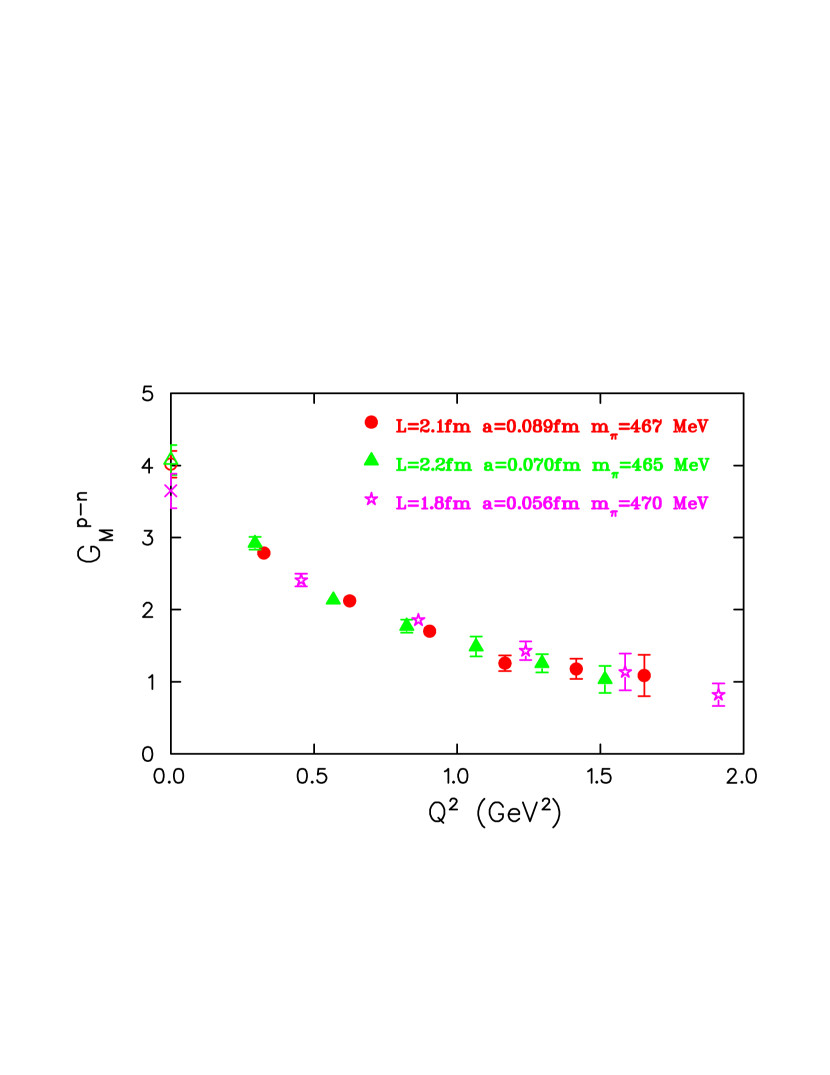
Figure 3: The nucleon isovector electric (upper) and magnetic (lower) form factors $G_{E}^{p-n}(Q^{2})$ and $G_{M}^{p-n}(Q^{2})$ at $m_{\pi}\sim 470$ MeV at $\beta=3.9$ (filled red circles), $4.05$ (filled green triangles) and $4.2$ (magenta stars) versus $Q^{2}$. The open symbols and crosses denoted the values at $Q^{2}=0$ at $\beta=3.9,4.05,$ and $4.2$ respectively, extracted by fitting the data to a dipole form.

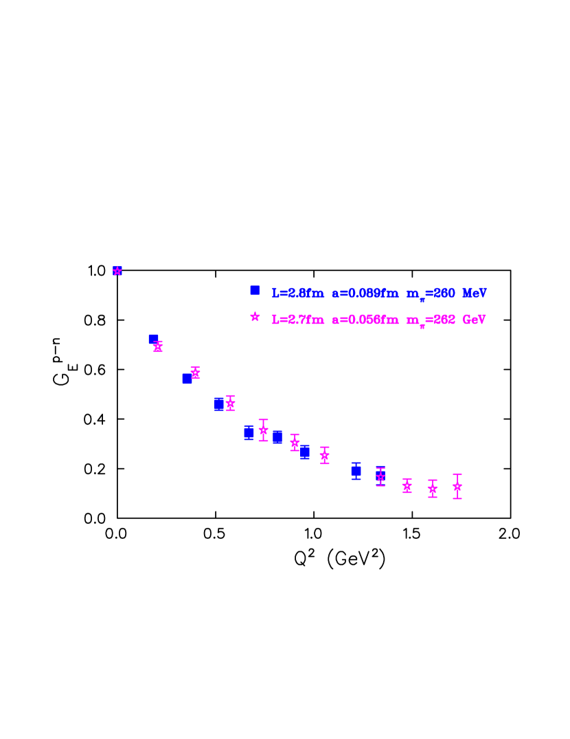
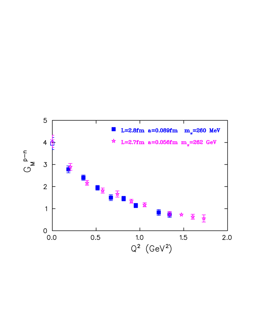
Figure 4: The nucleon isovector electric (upper) and magnetic (lower) form factors $G_{E}^{p-n}(Q^{2})$ and $G_{M}^{p-n}(Q^{2})$ at $m_{\pi}\sim 260$ MeV at $\beta=3.9$ (filled red circles) and $4.2$ (magenta stars) versus $Q^{2}$. The open symbols and crosses denoted the values at $Q^{2}=0$ at $\beta=3.9$ and $4.2$ respectively, extracted by fitting the data to a dipole form.

To assess cut-off effects we compare in Figs. 3 and 4 results for $G_{E}^{p-n}(Q^{2})$ and $G_{M}^{p-n}(Q^{2})$ for three different lattice spacings at a similar pion mass. We consider results at our heaviest and lightest pion masses. For $G_{M}^{p-n}(Q^{2})$, results at these three lattice spacings are consistent for both heavy and light mass indicating that cut-off effects are negligible for these lattice spacings at our current statistical precision. There is also consistency for the results obtained for $G_{E}^{p-n}(Q^{2})$ at the smaller pion mass of 260 MeV, as can be seen in Fig. 4. At the heavier pion mass of 470 MeV, a couple of data obtained on the finest lattice have higher values, which however are well within the statistical fluctuations.

III.3 Mass dependence of form factors

Our lattice simulations use light quark masses that correspond to pion masses in the range of about 470 MeV to 260 MeV. In order to obtain results at the physical point we need to study the dependence on the quark mass or equivalently on the pion mass. We show in Fig. 5 the dependence on the pion mass at a fixed volume and lattice spacing. We show both $G_{E}^{p-n}$ and $G_{M}^{p-n}$ computed at several values of the pion mass spanning pion masses from about 470 MeV to 300 MeV at $\beta=3.9$.

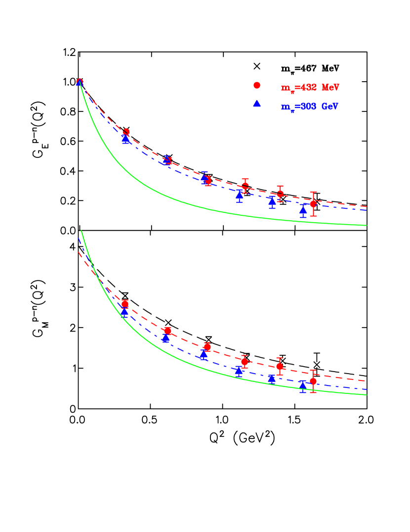
Figure 5: The nucleon form factors $G_{E}^{p-n}(Q^{2})$ and $G_{M}^{p-n}(Q^{2})$ at $\beta=3.9$ for $m_{\pi}=468$ MeV (crosses), $m_{\pi}=432$ MeV (filled red circles) and $m_{\pi}=303$ MeV (filled blue triangles) versus $Q^{2}$. The dashed lines are the result of a dipole fit to the lattice data.The solid line is J. Kelly’s parametrization to the experimental data Kelly (2004).

In order to extract the anomalous magnetic moment and mean squared radii we need to perform a fit to the $Q^{2}$-dependence of the form factors. For both $G_{E}^{p-n}(Q^{2})$ and $G_{M}^{p-n}(Q^{2})$ we use a dipole of the form given in Eq. (22). We fit the lattice data using all data up to a largest $Q^{2}$ value of $\sim 1.5$ GeV². These fits, shown in Fig. 5, describe the results very well. On the same figures we also show Kelly’s parametrization of the experimental data Kelly (2004). Although the mass dependence is weak and lattice data show a weaker $Q^{2}$-dependence than experimental data, the general trend is that lattice results approach experiment as the light quark mass decreases towards its physical value. The values extracted from the fits for the dipole electric and magnetic masses, $m_{E}$ and $m_{M}$, are therefore larger than in experiment which is expected given the smaller slope exhibited by the lattice data. As we discuss in the next section, this behavior is observed with other lattice discretization schemes as well. In Table 2 we tabulate the resulting fitting parameters for all $\beta$ and $\mu$ values. The parameters $m_{E}$, $G_{M}(0)$ and $m_{M}$ have been extracted from fits to the form given in Eq. (22).

$a\mu$	$m_{\pi}$ (GeV)	$m_{E}$ (GeV)	$G_{M}(0)$	$m_{M}$ (GeV)	$\mu_{N}$
$\beta=3.9$
0.0100	0.4675	1.40(7)	4.02(18)	1.62(17)	2.57(22)
0.0085	0.4319	1.33(10)	3.86(25)	1.45(21)	2.49(28)
0.0064	0.3770	1.19(9)	3.91(35)	1.69(36)	2.70(33)
0.004	0.3032	1.16(10)	4.20(41)	1.01(14)	2.20(26)
0.004	0.2978	0.98(6)	3.99(35)	1.11(16)	2.13(18)
0.003	0.2600	1.03(6)	3.95(27)	1.13(13)	2.14(12)
$\beta=4.05$
0.008	0.4653	1.41(74)	4.07(21)	1.56(19)	2.53(49)
0.006	0.4035	1.24(10)	4.26(30)	1.43(20)	2.41(21)
0.003	0.2925	1.31(18)	4.13(62)	1.09(27)	2.16(14)
$\beta=4.2$
0.0065	0.4698	1.75(12)	3.65(24)	2.09(31)	2.62(24)
0.002	0.2622	1.12(8)	4.05(28)	1.17(12)	1.84(17)

Table 2: Results on the nucleon electric and magnetic mass extracted by fitting to a dipole form. The two last column give the $G_{M}(0)$ and the nucleon anomalous magnetic moment in Bohr magnetons by fitting $G_{M}^{p-n}(Q^{2})$ to the dipole form given in Eq. (22).

III.4 Comparison of lattice results

We have shown that volume and cut-off effects are small on the isovector form factors for the parameters used in our simulations. This justifies to some extent a comparison with results of other collaborations that use different fermions but in a similar volumes and at a similar lattice spacings. In Figs. 6 and 7 we show a comparison of the results of this work with those obtained using $N_{F}=2+1$ dynamical domain wall fermions (DWF) Syritsyn et al. (2010), $N_{F}=2$ Wilson improved Clover fermions  Capitani et al. (2010) and using a hybrid action of tadpole-improved $N_{F}=2+1$ staggered fermions and domain wall valence quarks Bratt et al. (2010) for a pion mass around 300 MeV. We can see a nice agreement among all lattice results for $G_{E}^{p-n}$. As already pointed out, all lattice results show a weaker $Q^{2}$-dependence than experiment. We would like to note that in Ref. Bratt et al. (2010) hybrid results for $m_{\pi}=356$ MeV are obtained on a lattice of $L=2.5$ and $L=3.5$ fm. A comparison between these results showed volume effects for the isovector $F_{1}$ but not for the isovector $F_{2}$. This is consistent with our results on the isovector electric and magnetic form factors shown in Fig. 2. The experimental data are obtained by interpolating the neutron form factors to the $Q^{2}$-values of the proton form factors as described in ref. Alexandrou et al. (2006). In the case of $G_{M}^{p-n}$ there are discrepancies, in particular, with the results using Clover fermions which are systematically lower. We note that compared to $G_{E}^{p-n}$, $G_{M}^{p-n}$ is more sensitive to the nucleon mass which is needed as an input. Clearly one has to study further the systematics on the various lattice results, some of which are still preliminary, in order to clarify these discrepancies.

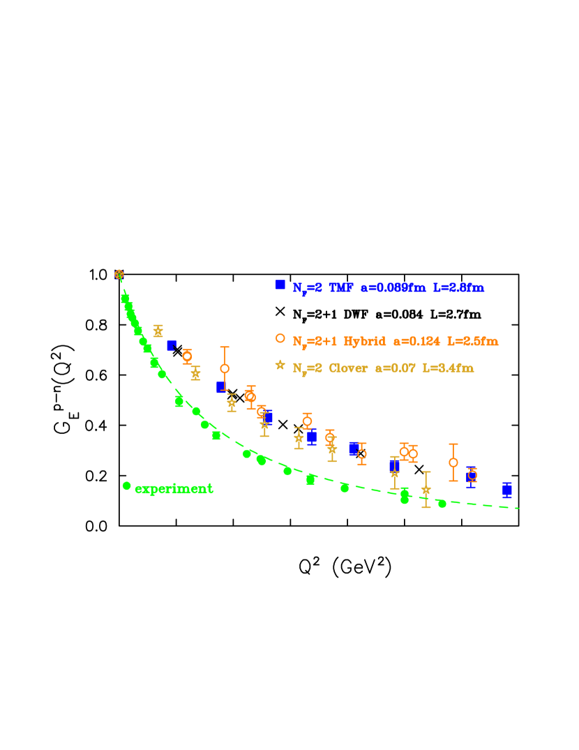
Figure 6: Isovector electric form factor $G_{E}^{p-n}(Q^{2})$ as a function of $Q^{2}$. $N_{F}=2$ TMF results at $m_{\pi}=298$ MeV are shown with filled squares, $N_{F}=2+1$ DWF Syritsyn et al. (2010) (crosses), hybrid Bratt et al. (2010) (open orange circles) and Clover fermions Capitani et al. (2010) (yellow stars). Experimental data are shown with the filled green circles accompanied with Kelly’s parametrization shown with the dashed line.

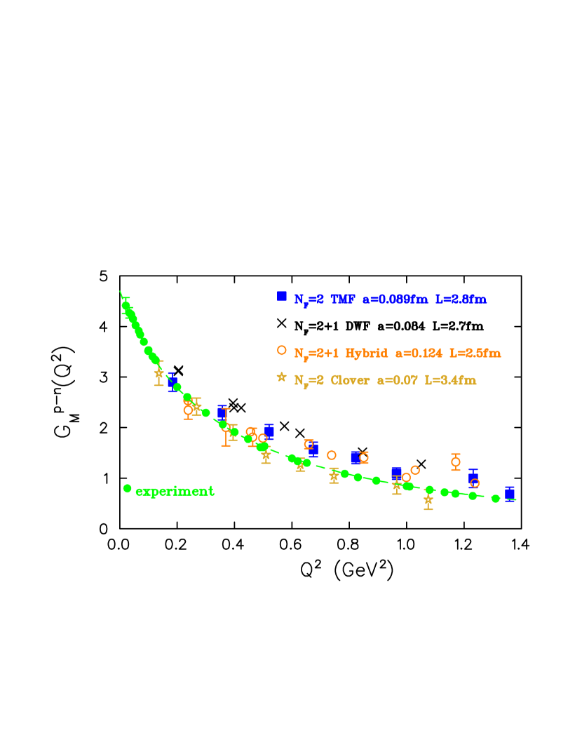
Figure 7: Isovector magnetic form factor $G_{M}(Q^{2})$ as a function of $Q^{2}$. The notation is the same as that of Fig. 6.

III.5 Chiral extrapolation

Given that cut-off effects are small, we use chiral perturbation theory that holds in the continuum to study the quark mass dependence of the electromagnetic form factors down to the physical point. This will be justified in the next section where we discuss the continuum extrapolation of our results. For the chiral extrapolation, we use our TMF results that cover a range of pion masses from about 470 MeV down to about 260 MeV. The pion mass dependence for the isovector form factors as well as for the anomalous magnetic moment and radii have been studied within HB$\chi$PT in the so called small scale expansion (SSE) formulation Hemmert and Weise (2002).

The anomalous magnetic moment, which is given by the isovector Dirac form factor $F_{2}(0)$ is extracted by fitting the $Q^{2}$ assuming e.g. a dipole form dependence. The slope of $F_{1}$ at $Q^{2}=0$ determines the transverse size of the hadron, $<r_{\perp}^{2}>=-4dF_{1}/dQ^{2}|_{Q^{2}=0}$. In the non-relativistic limit the root mean square (r.m.s.) radius is related to the slope of the form factor at zero momentum transfer. Therefore the r.m.s. radii can be obtained from the values of the dipole masses by using

$$<r_{i}^{2}>=-\frac{6}{F_{i}(Q^{2})}\frac{dF_{i}(Q^{2})}{dQ^{2}}|_{Q^{2}=0}=\frac{12}{m_{i}}\hskip 14.22636pti=1,2\quad.$$ (23)

The electric and magnetic radii are given by $<r_{e,m}^{2}>=12/m_{E,M}$ and can be directly evaluated from the values given in Table 2.

Using HB$\chi$PT to one-loop, with $\Delta$ degrees of freedom and iso-vector $N$-$\Delta$ coupling included in LO Hemmert and Weise (2002); Gockeler et al. (2005) the expression for the isovector anomalous magnetic moment $\kappa^{p-n}$ is given by Gockeler et al. (2005)

$$\kappa^{p-n}(m_{\pi}) = {\ \kappa_{\rm v}(0)}-\frac{g_{A}^{2}m_{\pi}m_{N}}{4\pi f_{\pi}^{2}}$$ (24)

$$+\frac{2{c_{A}^{2}}\Delta m_{N}}{9\pi^{2}f_{\pi}^{2}}\biggl{[}\sqrt{1-\frac{m_{\pi}^{2}}{\Delta^{2}}}\log R(m_{\pi})+\log\left(\frac{m_{\pi}}{2\Delta}\right)\biggr{]}$$

$$-8{E_{1}}m_{N}m_{\pi}^{2}+\frac{4c_{A}c_{V}g_{A}m_{N}m_{\pi}^{2}}{9\pi^{2}f_{\pi}^{2}}\log\left(\frac{2\Delta}{\lambda}\right)$$

$$+\frac{4{c_{A}}{c_{V}}g_{A}m_{N}m_{\pi}^{3}}{27\pi F_{\pi}^{2}\Delta}-\frac{8{c_{A}c_{V}}g_{A}\Delta^{2}m_{N}}{27\pi^{2}f_{\pi}^{2}}$$

$$\biggl{[}\left(1-\frac{m_{\pi}^{2}}{\Delta^{2}}\right)^{3/2}\log R(m_{\pi})$$

$$+ \left(1-\frac{3m_{\pi}^{2}}{2\Delta^{2}}\right)\log\left(\frac{m_{\pi}}{2\Delta}\right)\biggr{]}\,,$$

and for the isovector Dirac form factor Gockeler et al. (2005)

$$F_{1}^{p-n}(m_{\pi},Q^{2})=1+\frac{1}{(4\pi f_{\pi})^{2}}\left\{-Q^{2}\left(\frac{68}{81}c_{A}^{2}-\frac{2}{3}g_{A}^{2}-2B_{10}(\lambda)\right)\right.-Q^{2}\left(\frac{40}{27}c_{A}^{2}-\frac{5}{3}g_{A}^{2}-\frac{1}{3}\right)\log\left[\frac{m_{\pi}}{\lambda}\right]$$

$${}+\int_{0}^{1}dx\left[\frac{16}{3}\Delta^{2}c_{A}^{2}+m_{\pi}^{2}\left(3g_{A}^{2}+1-\frac{8}{3}c_{A}^{2}\right)\right.+\left.Q^{2}x(1-x)\left(5g_{A}^{2}+1-\frac{40}{9}c_{A}^{2}\right)\right]\log\left[\frac{\tilde{m}^{2}}{m_{\pi}^{2}}\right]$$

$${}+\int_{0}^{1}dx\left[-\frac{32}{9}c_{A}^{2}Q^{2}x(1-x)\frac{\Delta\log R(\tilde{m})}{\sqrt{\Delta^{2}-\tilde{m}^{2}}}\right]$$

$${}-\left.\int_{0}^{1}dx\;\frac{32}{3}c_{A}^{2}\Delta\left[\sqrt{\Delta^{2}-m_{\pi}^{2}}\log R(m_{\pi})-\sqrt{\Delta^{2}-\tilde{m}^{2}}\log R(\tilde{m})\right]\right\}+\mathcal{O}(\epsilon^{4})\,.$$ (25)

To the same order the expansion of the isovector Pauli form factor is given by

$$F_{2}^{p-n}(m_{\pi},Q^{2})=\kappa^{p-n}(m_{\pi})-g_{A}^{2}\frac{4\pi m_{N}}{(4\pi f_{\pi})^{2}}\int_{0}^{1}dx\left[\sqrt{\tilde{m}^{2}}-m_{\pi}\right]{}+\frac{32c_{A}^{2}m_{N}\Delta}{9(4\pi f_{\pi})^{2}}\int_{0}^{1}dx\left[\frac{1}{2}\log\left[\frac{\tilde{m}^{2}}{4\Delta^{2}}\right]-\log\left[\frac{m_{\pi}}{2\Delta}\right]\right.\\ \left.{}+\frac{\sqrt{\Delta^{2}-\tilde{m}^{2}}}{\Delta}\log R(\tilde{m})-\frac{\sqrt{\Delta^{2}-m_{\pi}^{2}}}{\Delta}\log R(m_{\pi})\right]\,,$$ (26)

where

$$R(m)=\frac{\Delta}{m}+\sqrt{\frac{\Delta^{2}}{m^{2}}-1}\,,\quad\tilde{m}^{2}=m_{\pi}^{2}+Q^{2}x(1-x)\,.$$ (27)

We perform a fit to $F_{1}(m_{\pi},Q^{2})$ and $F_{2}(m_{\pi},Q^{2})$ with five parameters, namely the iso-vector magnetic moment at the chiral limit $\kappa_{\rm v}(0)$, the isovector and axial N to $\Delta$ coupling constants, $c_{V}$ and $c_{A}$ and the two counterterms $B_{10}(\lambda)$ and $E_{1}(\lambda)$. The rest of the parameters are fixed to their physical values, namely $m_{N}=0.938$ MeV, $g_{A}=1.267$, $f_{\pi}=0.0924$ MeV and the $\Delta$-nucleon mass splitting $\Delta=0.2711$. The counterterms are evaluated at $\lambda=0.6$ GeV. For the chiral extrapolation we use data at the three lowest $Q^{2}$-values. As can be seen in Fig. 8, the chiral extrapolation decreases the value of $F_{1}$ and increases the value of $F_{2}$ at low $Q^{2}$, bringing them into qualitative agreement with experiment. The values of the fit parameters are given in Table 3. Although such a chiral extrapolation is useful and probes the general trend we would like to point out that the $\chi^{2}$ per degree of freedom (d.o.f) is 4.3, which means that the description of the results is not really optimal.

Fit parameter	data at 3 $\beta$ values	continuum data
Fit separately $\kappa^{p-n}$, $r_{1}^{2\,p-n}$ and $r_{2}^{2\,p-n}$
$\kappa_{\rm v}(0)$	4.22(84)	4.22(74)
$c_{V}$	-5.86(3.52)	-5.46(2.73)
$E_{1}(0.6\,{\rm GeV})$	-8.95(3.80)	-8.58(3.00)
$B_{10}(0.6\,{\rm GeV})$	0.04(2)	0.04(2)
$B_{c2}(0.6\,{\rm GeV})$	0.14(3)	0.12(3)
Fit to the Dirac and Pauli form factors
$\kappa_{\rm v}(0)$	5.57(56)	5.20 (20)
$c_{A}$	1.56(3)	1.53(2)
$c_{V}$	-2.20(1.62)	-3.25(53)
$E_{1}(0.6\,{\rm GeV})$	-6.45(2.42)	-7.87(69)
$B_{10}(0.6\,{\rm GeV})$	1.21(6)	1.11(6)

Table 3: The values of the parameters extracted from the fit to $F_{1}$ and $F_{2}$ using lattice data at $\beta=3.9$, $\beta=4.05$ and $\beta=4.2$ (second column) and using the data after taking the continuum limit (third column).

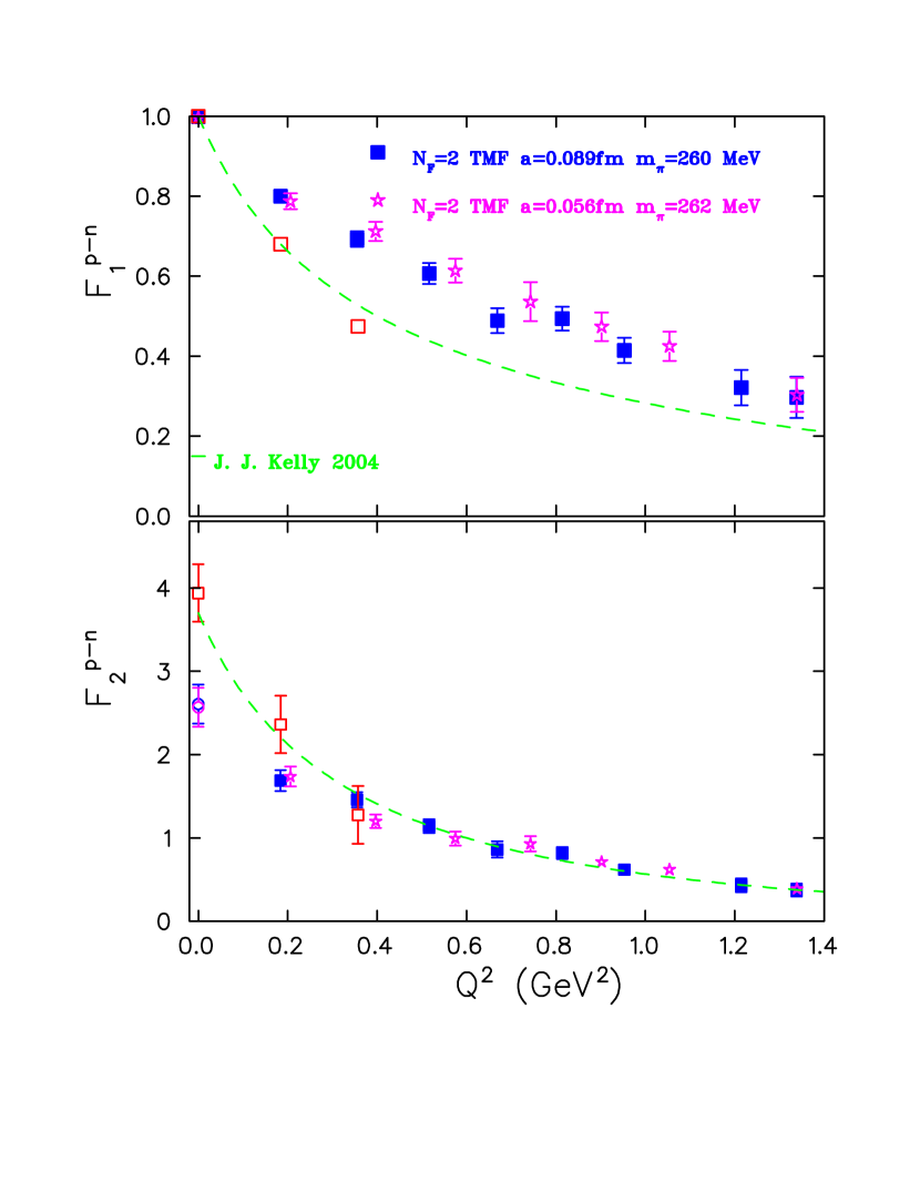
Figure 8: $F_{1}$ and $F_{2}$ for the coarser and finer lattices at pion mass of about 260 MeV. The dashed line is Kelly’s parametrization to the experimental data. The open squares show the values of $F_{1}$ and $F_{2}$ after chiral extrapolation to the physical point.

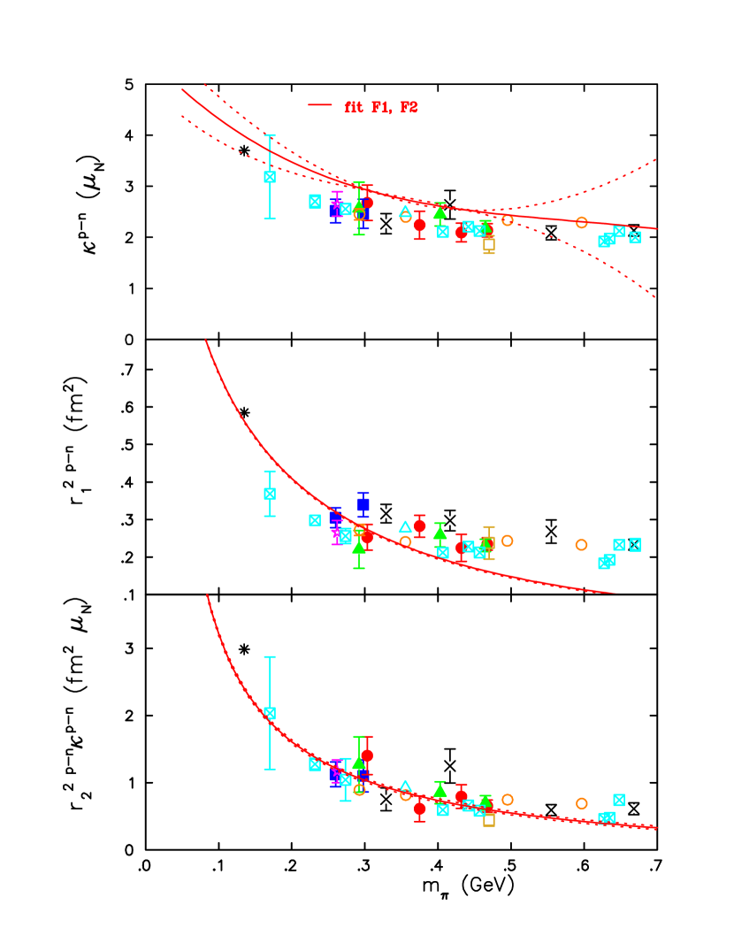
Figure 9: Chiral fits using the parameters determined from fitting $F_{1}$ and $F_{2}$. We show lattice data using $N_{F}=2$ TMF Alexandrou et al. (2010) ($a=0.089$ fm: filled red circles for $L=2.1$ fm and filled blue squares for $L=2.8$ fm; $a=0.070$ fm: filled green triangles for $L=2.2$ fm; $a=0.056$ fm: purple star for $L=2.7$ fm and open yellow square for $L=1.8$ fm), $N_{F}=2+1$ DWF Yamazaki et al. (2009) (crosses for $a=0.114$ fm and $L=2.7$ fm), $N_{F}=2+1$ using DWF and staggered sea Bratt et al. (2010) ($a=0.124$ fm: open orange circles for $L=2.5$ fm and open cyan triangle for $L=3.5$ fm) and using $N_{F}=2$ Clover fermions Collins et al. (2011) are also shown with the cyan cross-in-square symbols. The physical point is marked by the asterisk.

Using the fit parameters determined from $F_{1}$ and $F_{2}$ we can obtain the mass dependence of the isovector magnetic moment and radii. The expressions for the radii $r_{1}^{2\,p-n}$ and $r_{2}^{2\,p-n}$ are given by Gockeler et al. (2005)

$$r_{1}^{2} = -\frac{1}{(4\pi f_{\pi})^{2}}\biggl{[}1+7g_{A}^{2}+\left(10g_{A}^{2}+2\right)\log\left(\frac{m_{\pi}}{\lambda}\right)\biggr{]}$$ (28)

$$- \frac{12B_{10}}{(4\pi f_{\pi})^{2}}+\frac{{c_{A}^{2}}}{54\pi^{2}f^{2}_{\pi}}\biggl{[}26+30\log\left(\frac{m_{\pi}}{\lambda}\right)$$

$$+ 30\frac{\Delta}{\sqrt{\Delta^{2}-m_{\pi}^{2}}}\log R(m_{\pi})\biggr{]}$$

$$r_{2}^{2} = \frac{1}{\kappa_{\rm v}(m_{\pi})}\biggl{\{}\frac{g_{A}^{2}m_{N}}{8f_{\pi}^{2}\pi m_{\pi}}+\frac{c_{A}^{2}m_{N}}{9f^{2}_{\pi}\pi^{2}\sqrt{\Delta^{2}-m_{\pi}^{2}}}\log R(m_{\pi})$$ (29)

$$+ 24m_{N}{\ B_{c2}}\biggr{\}}$$

These are shown in Fig. 9 and the values obtained at the physical point are in agreement with experiment, which again indicates that the chiral extrapolation of the form factors could bring lattice data into agreement with experiment.

Alternately, fitting only $\kappa^{p-n}$ using three parameters, namely $\kappa_{\rm v}(0)$, $c_{V}$ and $E_{1}(\lambda=0.6\,{\rm GeV})$ and fixing $c_{A}=1.125$ yields $\chi^{2}/{\rm d.o.f.}=0.5$ and provides a nice fit to the results on $\kappa^{p-n}$. The Dirac radius $r_{1}^{2\,p-n}$ has only one fit parameter, whereas the combination $r_{2}^{2\,p-n}\kappa^{p-n}$ at leading one-loop order would be predicted since the term proportional to $B_{c2}$ would be absent. However, one can allow for such a term, which parametrizes the short-distance contributions to the Pauli radius and which can be regarded analogously to $B_{10}(\lambda)$ in the Dirac radius Gockeler et al. (2005). We perform a fit to $r_{1}^{2\,p-n}$ with fit parameter $B_{10}$ and to $r_{2}^{2\,p-n}\kappa^{p-n}$ with fit parameter $B_{c2}$ using the expressions of Eq. (29). The resulting values of the parameters from fitting $\kappa^{p-n}$, $r_{1}^{2\,p-n}$ and $r_{2}^{2\,p-n}\kappa^{p-n}$ independently are given in Table 3. If one treats $c_{A}$ as a fit parameter and performs a combined fit with six parameters to $\kappa^{p-n}$, $r_{1}^{2\,p-n}$ and $r_{2}^{2\,p-n}\kappa^{p-n}$ one obtains $\chi^{2}/{\rm d.o.f}=1.6$. The resulting fit for $\kappa^{p-n}$ is the same as that obtained by fitting separately the data on $\kappa^{p-n}$. The value of $\kappa^{p-n}$ at the physical point extracted from fitting the $F_{1}$ and $F_{2}$ agrees best with the physical value. This is also true for the Dirac radius, whereas for the Pauli radius the deviation from the physical value is larger. Omitting the term proportional to $B_{c2}$ in the Pauli radius increases the value of $\chi^{2}/{\rm d.o.f}$ and the resulting fits are similar except for the Dirac radius above pions of about 300 MeV.

IV Results in the continuum limit

In order to study the dependence on the lattice spacing quantitatively we use the simulations at three lattice spacings at the smallest and largest pion mass used in this work. We take as reference pion mass the one computed on the finest lattice and interpolate results at the other two $\beta$-values to these two reference masses. In Fig. 10 we show the value of the Dirac and Pauli $F_{1}$ and $F_{2}$ at these reference pion masses computed in units of $r_{0}$. We note that we first interpolate these form factors to the same value of $Q^{2}$. In the figure we show the form factors at $Q^{2}=0.357$ GeV. We perform a fit to these data using a linear form $F_{1}(a^{2})=F1(0)+c(a/r_{0})^{2}$. The resulting fit is shown in Fig. 10. Setting $c=0$ we obtain the constant line also shown in the figure. As can be seen, for both large and small pion masses the slope is consistent with zero yielding a value in the continuum limit in agreement with the constant fit. Therefore, we conclude that finite $a$ effects are negligible and for the intermediate pion masses we obtain the values in the continuum by fitting our data at $\beta=3.9$ and $\beta=4.05$ to a constant.

$r_{0}m_{\pi}$	$\kappa^{p-n}$
	$(\beta=3.9)$	$(\beta=4.05)$	$(\beta=4.2)$	$(a\rightarrow 0)$
1.1019	2.12(13)	2.13(15)	1.84(17)	2.05(8) [1.79(26)]
1.0	2.08(18)	2.36(23)		2.18(14)
0.95	2.09(21)	2.42(22)		2.25(15)
0.85	2.27(27)	2.53(26)		2.41(19)
0.686	2.34(36)	2.54(51)		2.40(29)
0.615	2.49(23)	2.57(53)	2.62(24)	2.55(16) [2.71(41)]

Table 4: In the second, third and fourth column we give the interpolated values of $\kappa^{p-n}$ at the value of $m_{\pi}r_{0}$ given in the first column. We used $r_{0}/a=5.22(2)$, $6.61(3)$ and $8.31(5)$ for $\beta=3.9$, $4.05$ and $4.2$, respectively. In the fifth column we give the value of $\kappa^{p-n}$ after extrapolating to $a=0$ using a constant fit. In the parenthesis we give the corresponding values when using a linear fit.

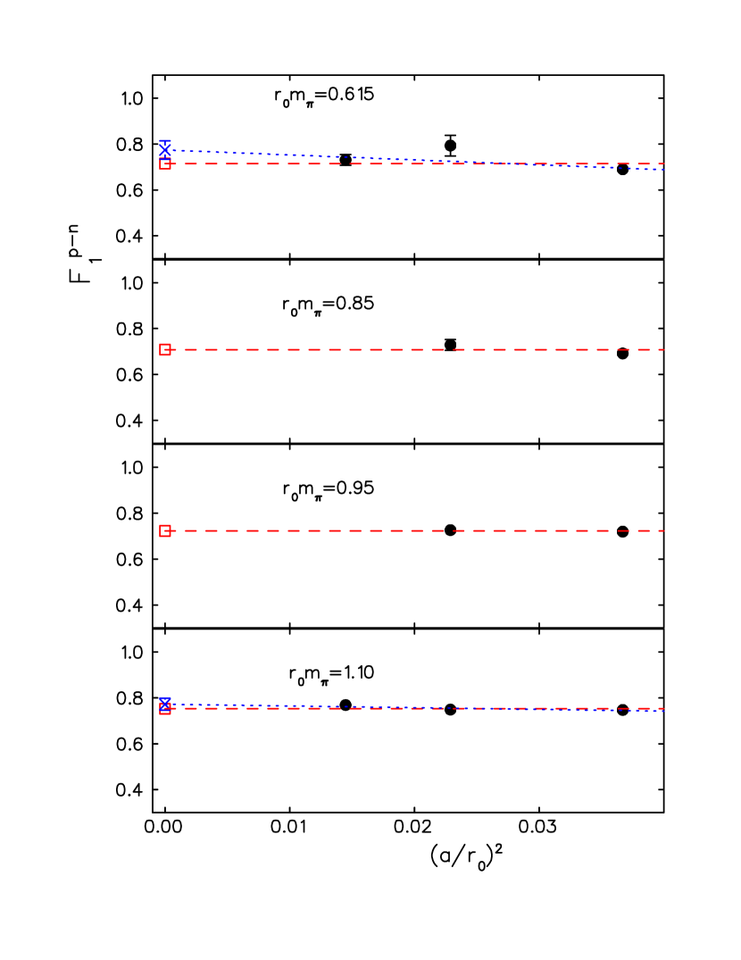
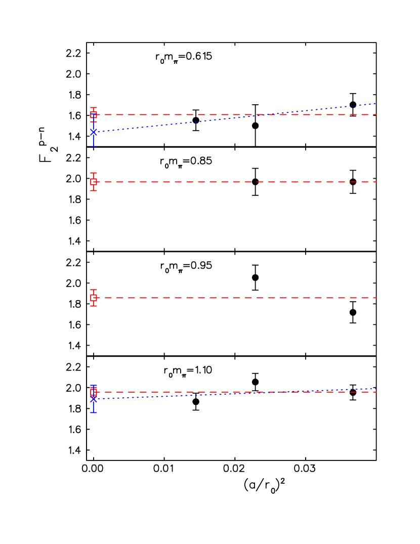
Figure 10: Continuum results for the isovector Dirac and Pauli form factors $F_{1}$ and $F_{2}$ at $Q^{2}=357$ GeV². The dashed line is a fit to a constant, whereas the dotted line is a fit to a line.

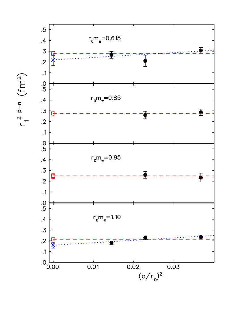
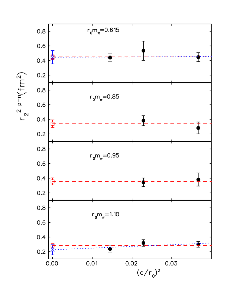
Figure 11: Continuum results for the isovector Dirac and Pauli mean squared radii $r_{1}^{2\,p-n}$ and $r_{2}^{2\,p-n}$. The notation is the same as in Fig. 10.

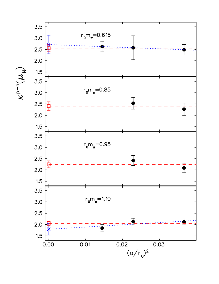
Figure 12: Continuum results for the nucleon anomalous magnetic moment $\kappa^{p-n}$. The notation is the same as in Fig. 10.

In Figs. 11 and . 12 a we show the continuum extrapolation of the r.m.s Dirac and Pauli radii and the anomalous magnetic moment, respectively. The corresponding values of $\kappa^{p-n}$ at the six reference pion masses used in the figures are given in Table 4 and those of the Dirac and Pauli mean square radii in Table 5.

Having results in the continuum limit we can now perform the chiral fits described in the previous section. We show these chiral fits to the continuum results for the anomalous magnetic moment and Dirac and Pauli mean square radii in Figs. 13, 14 and 15.

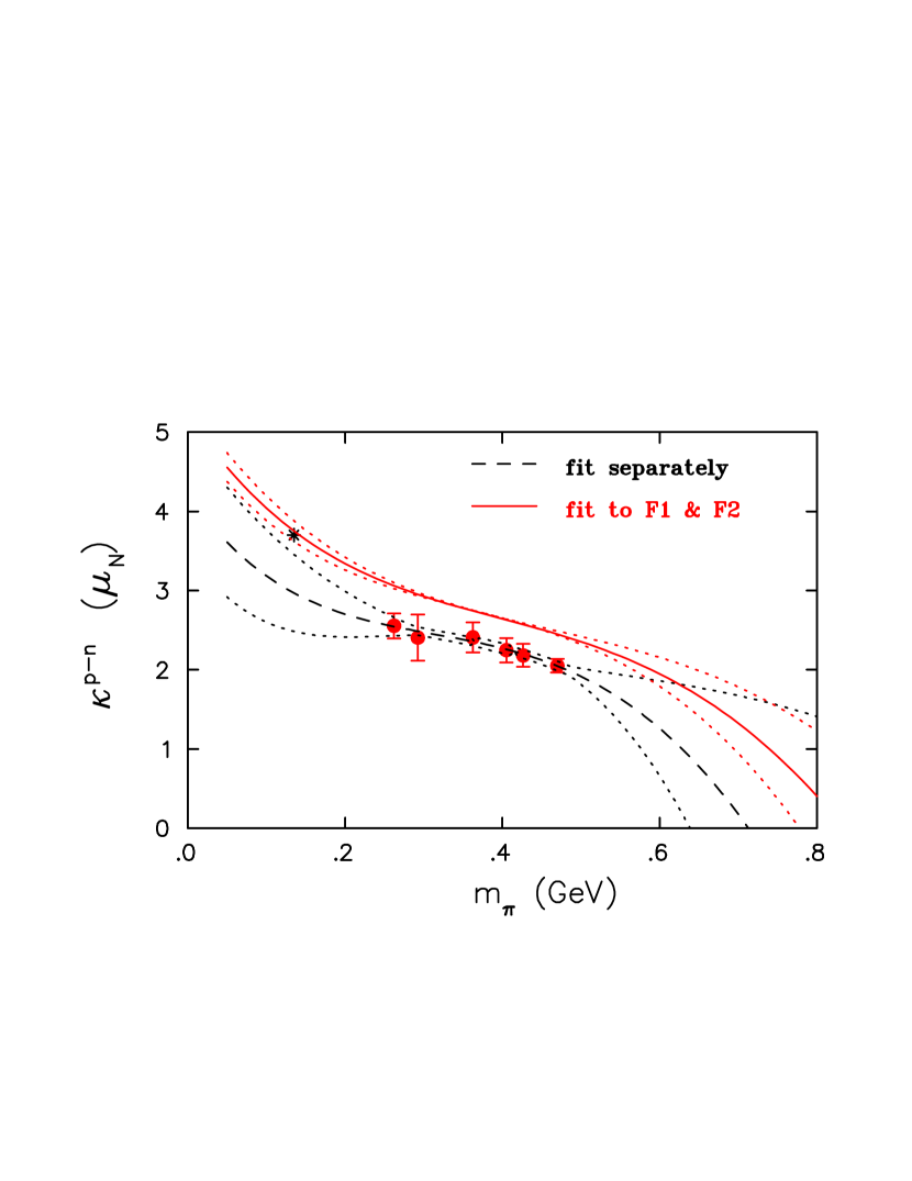
Figure 13: Chiral extrapolation of the results on the nucleon anomalous magnetic moment $\kappa^{p-n}$ after taking the continuum limit. The dashed line is obtained by fitting $\kappa^{p-n}$ independently, whereas the solid line is the result of fitting the Dirac and Pauli form factors.

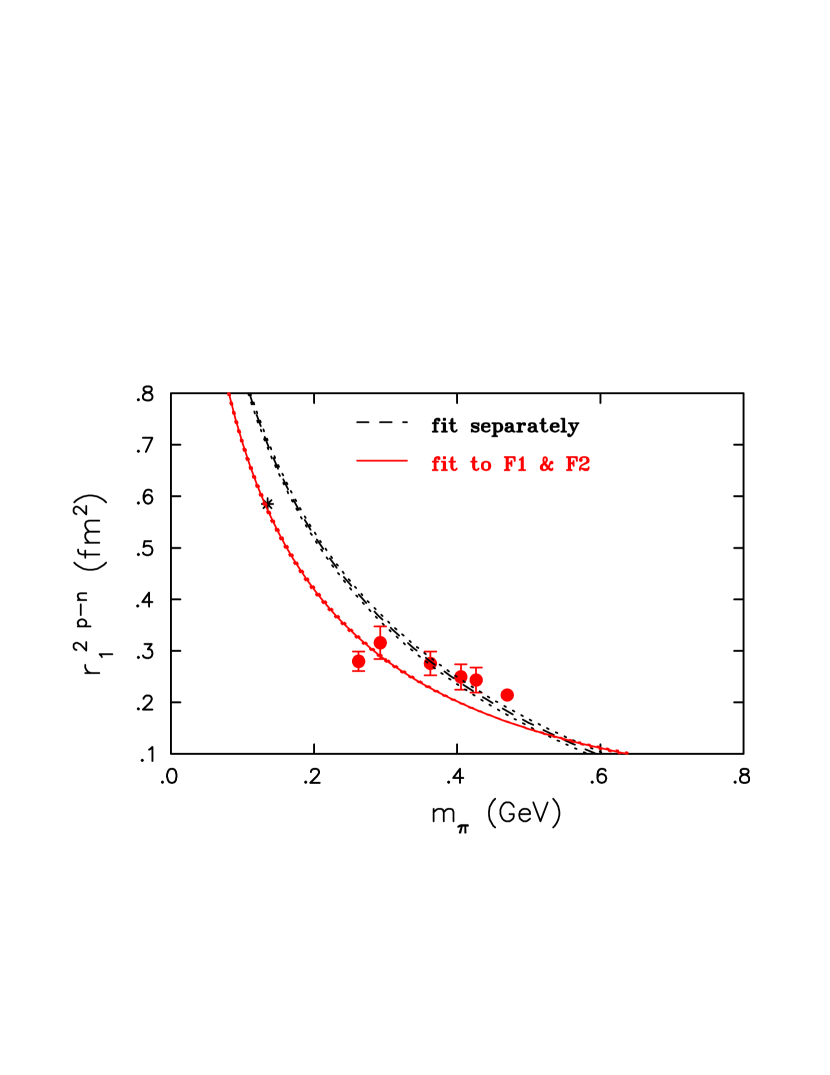
Figure 14: As in Fig. 13 but for $r_{1}^{2\,p-n}$.

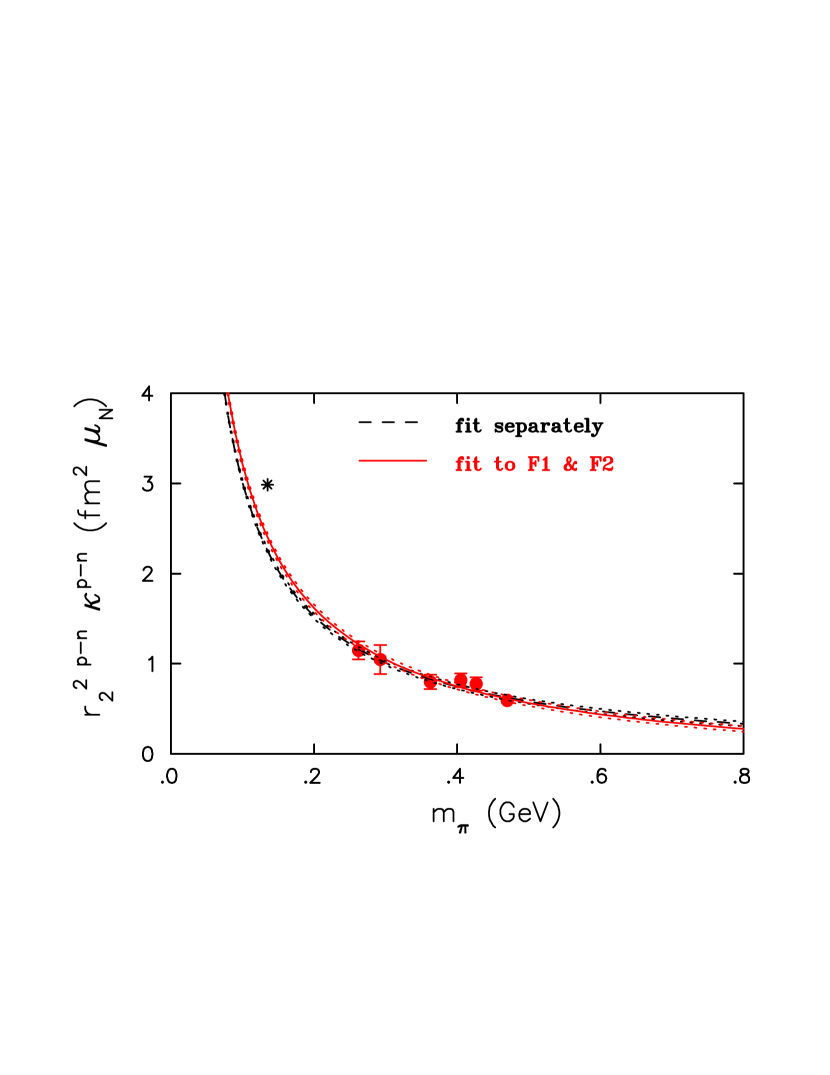
Figure 15: As in Fig. 13 but for $r_{2}^{2\,p-n}\kappa^{p-n}$.

The behavior observed is similar to that obtained when using the raw lattice data. Namely, chiral fits to the Dirac and Pauli form factors $F_{1}$ and $F_{2}$ bring agreement with experiment at low $Q^{2}$-values, and therefore the values for $\kappa^{p-n}$ and $r_{1}^{2\,p-n}$ derived using the parameters of the chiral fit to $F_{1}$ and $F_{2}$ agree with the the experimental values. The description of $r_{2}^{2\,p-n}$ is also reasonable bringing lattice results close to the value obtained at the physical point, although not fully reproducing the experimental value. In the figures we also include the curves obtained by fitting separately the anomalous magnetic moment and radii. For the former the mean value obtained at the physical point is lower as compared to the value obtained from fitting $F_{1}$ and $F_{2}$, with, however, almost overlapping errors. For the Pauli mean squared radius the fits are almost identical, whereas for the Dirac radius both fits do not provide a good description to our lattice results. The parameters extracted from the chiral fits to the continuum extrapolated results are in fact in agreement with those determined using lattice data at the different $\beta$-values, as can be seen from the values given in Table 3. This is an a posteriori justification of using the continuum HB perturbation expressions to fit the lattice data at finite lattice spacing.

$r_{0}m_{\pi}$	$r_{1}^{2\,p-n}$	$r_{2}^{2\,p-n}$	$r_{1}^{2\,p-n}$	$r_{2}^{2\,p-n}$	$r_{1}^{2\,p-n}$	$r_{2}^{2\,p-n}$	$r_{1}^{2\,p-n}$	$r_{2}^{2\,p-n}$
	$(\beta=3.9)$		$(\beta=4.05)$		$(\beta=4.2)$		$(a\rightarrow 0)$
1.1019	0.236(17)	0.300(39)	0.229(17)	0.319(45)	0.183(16)	0.238(43)	0.214(9)[0.160(39)]	0.285(24) [0.226(70)]
1.0	0.226(36)	0.379(79)	0.258(33)	0.326(62)			0.243(24)	0.347(49)
0.95	0.234(41)	0.382(89)	0.259(32)	0.345(59)			0.249(25)	0.356(49)
0.85	0.286(30)	0.282(81)	0.261(35)	0.382(68)			0.276(23)	0.340(52)
0.686	0.378(41)	0.409(99)	0.221(50)	0.494(126)			0.442(78)	0.442(78)
0.615	0.307(27)	0.446(61)	0.210(53)	0.534(132)	0.266(32)	0.441(50)	0.280(17) [0.220(54)]	0.450(37) [0.445(91)]

Table 5: In the second, third and fourth raws we give the interpolated values of $r_{1}^{2\,p-n}$ and $r_{2}^{2\,p-n}$in fm² at the value of $m_{\pi}r_{0}$ given in the first column. We used $r_{0}/a=5.22(2)$, $6.61(3)$ and $8.31(5)$ for $\beta=3.9$, $4.05$ and $4.2$, respectively. In the fifth raws we give the value of $r_{1}^{2\,p-n}$ and $r_{2}^{2\,p-n}$ after extrapolating to $a=0$ using a constant fit. In the parenthesis we give the corresponding values when using a linear fit.

V Conclusions

Computing the electromagnetic form factors of the nucleon directly from the fundamental theory of the strong interactions has been the goal of hadron physics since the discovery of QCD. Within the lattice formulation this goal is now being realized. Comparing lattice results with a number of different fermion discretization schemes we find an overall agreement. In this work we use dynamical simulations of two-degenerate flavors of light quarks in the twisted mass formulation of QCD, which at maximal twist is automatically ${\cal O}(a^{2})$ improved, thus requiring no improvement on the operator level. We use light quark masses yielding pion masses in the range of about 260 MeV up to 470 MeV. Even for our lightest pion mass of 260 MeV the form factors decrease slower with increasing momentum transfer squared than form factors obtained from experiments. In this work we examine both volume and cut-off effects to identify the source of this discrepancy. We also examine the pion mass dependence of the form factors as well as of the quantities derived by fitting the $Q^{2}$-dependence of these form factors.

By comparing results at two different volumes we find that for $Lm_{\pi}\stackrel{{\scriptstyle>}}{{\sim}}3.3$ any volume effects are within our statistical accuracy for the magnetic form factor. A small volume dependence is seen in the case of the electric form factor that indicates an increase in the slope as the volume increases. By considering the continuum limit using results at three lattice spacings we also show that, cut-off effects are small for lattice spacings less than about 0.1 fm. The pion mass dependence is examined using HB effective theory with explicit $\Delta$-degrees of freedom. Fitting the isovector Dirac and Pauli form factors at low $Q^{2}$ we show that the chiral extrapolated data agree with experiment. This is true when using the lattice results at the three $\beta$-values as well as when using the lattice results after taking the continuum limit.

References

- Jones et al. (2000) M. K. Jones et al. (Jefferson Lab Hall A), Phys. Rev. Lett. 84, 1398 (2000), eprint nucl-ex/9910005.
- Gayou et al. (2002) O. Gayou et al. (Jefferson Lab Hall A), Phys. Rev. Lett. 88, 092301 (2002), eprint nucl-ex/0111010.
- Perdrisat et al. (2007) C. F. Perdrisat, V. Punjabi, and M. Vanderhaeghen, Prog. Part. Nucl. Phys. 59, 694 (2007), eprint hep-ph/0612014.
- Guichon and Vanderhaeghen (2003) P. A. M. Guichon and M. Vanderhaeghen, Phys. Rev. Lett. 91, 142303 (2003), eprint hep-ph/0306007.
- de Jager (2008) K. de Jager, Nucl. Phys. A805, 494 (2008).
- Shindler (2008) A. Shindler, Phys. Rept. 461, 37 (2008), eprint 0707.4093.
- Frezzotti et al. (2001) R. Frezzotti, P. A. Grassi, S. Sint, and P. Weisz (Alpha), JHEP 0108, 058 (2001), eprint hep-lat/0101001.
- Frezzotti and Rossi (2004) R. Frezzotti and G. C. Rossi, JHEP 08, 007 (2004), eprint hep-lat/0306014.
- Weisz (1983) P. Weisz, Nucl. Phys. B212, 1 (1983).
- Alexandrou (2009) C. Alexandrou (2009), eprint 0906.4137.
- Alexandrou et al. (2009a) C. Alexandrou et al. (ETM), Phys. Rev. D80, 114503 (2009a), eprint 0910.2419.
- Drach et al. (2008) V. Drach et al., PoS LATTICE2008, 123 (2008), eprint 0905.2894.
- Alexandrou et al. (2008a) C. Alexandrou et al. (European Twisted Mass), Phys. Rev. D78, 014509 (2008a), eprint 0803.3190.
- Alexandrou et al. (2007) C. Alexandrou et al. (ETM Collaboration), PoS LAT2007, 087 (2007), eprint arXiv:0710.1173 [hep-lat].
- Drach et al. (2010) V. Drach et al., PoS Lattice 2010, 123 (2010).
- Alexandrou (2010) C. Alexandrou (ETM Collaboration), PoS Lattice 2010, 001 (2010).
- Alexandrou et al. (2009b) C. Alexandrou et al., PoS LAT2009, 145 (2009b), eprint 0910.3309.
- Alexandrou et al. (2008b) C. Alexandrou et al., PoS LAT2008 B414, 145 (2008b), eprint hep-lat/9211042.
- Alexandrou et al. (1994) C. Alexandrou, S. Gusken, F. Jegerlehner, K. Schilling, and R. Sommer, Nucl. Phys. B414, 815 (1994), eprint hep-lat/9211042.
- Gusken (1990) S. Gusken, Nucl. Phys. Proc. Suppl. 17, 361 (1990).
- Alexandrou et al. (2006) C. Alexandrou, G. Koutsou, J. W. Negele, and A. Tsapalis, Phys. Rev. D74, 034508 (2006), eprint hep-lat/0605017.
- Alexandrou et al. (2010) C. Alexandrou et al. (ETM) (2010), eprint 1012.0857.
- Urbach (2007) C. Urbach, PoS LAT2007, 022 (2007).
- Baron et al. (2010) R. Baron et al. (ETM), JHEP 08, 097 (2010), eprint 0911.5061.
- Kelly (2004) J. J. Kelly, Phys. Rev. C70, 068202 (2004).
- Syritsyn et al. (2010) S. N. Syritsyn et al., Phys. Rev. D81, 034507 (2010), eprint 0907.4194.
- Capitani et al. (2010) S. Capitani, M. Della Morte, B. Knippschild, and H. Wittig (2010), eprint 1011.1358.
- Bratt et al. (2010) J. D. Bratt et al. (LHPC), Phys. Rev. D82, 094502 (2010), eprint 1001.3620.
- Hemmert and Weise (2002) T. R. Hemmert and W. Weise, Eur. Phys. J. A15, 487 (2002), eprint hep-lat/0204005.
- Gockeler et al. (2005) M. Gockeler et al. (QCDSF), Phys. Rev. D71, 034508 (2005), eprint hep-lat/0303019.
- Yamazaki et al. (2009) T. Yamazaki et al., Phys. Rev. D79, 114505 (2009), eprint 0904.2039.
- Collins et al. (2011) S. Collins et al. (2011), eprint 1101.2326.