The pion-pion scattering amplitude. IV:
Improved analysis with once subtracted Roy-like equations up to 1100 MeV

Abstract

We improve our description of $\pi\pi$ scattering data by imposing additional requirements to our previous fits, in the form of once-subtracted Roy-like equations, while extending our analysis up to 1100 MeV. We provide simple and ready to use parametrizations of the amplitude. In addition, we present a detailed description and derivation of these once-subtracted dispersion relations that, in the 450 to 1100 MeV region, provide an additional constraint which is much stronger than our previous requirements of Forward Dispersion Relations and standard Roy equations. The ensuing constrained amplitudes describe the existing data with rather small uncertainties in the whole region from threshold up to 1100 MeV, while satisfying very stringent dispersive constraints. For the S0 wave, this requires an improved matching of the low and high energy parametrizations. Also for this wave we have considered the latest low energy $K_{\ell 4}$ decay results, including their isospin violation correction, and we have removed some controversial data points. These changes on the data translate into better determinations of threshold and subthreshold parameters which remove almost all disagreement with previous Chiral Perturbation Theory and Roy equation calculations below 800 MeV. Finally, our results favor the dip structure of the S0 inelasticity around the controversial 1000 MeV region.

I Introduction

In a series of papers Pelaez:2004vs ; Kaminski:2006yv ; Kaminski:2006qe that we will denote by PY05, KPY06 and KPY08, respectively, we have provided several sets of precise phenomenological fits to $\pi\pi$ scattering data. The interest in a precise and model independent description of the data available in this process is twofold: On the one hand, it could be used at low energies to extract information about the parameters of Chiral Perturbation Theory (ChPT) Gasser:1983yg , quark masses and the size of the chiral condensate, pionic atom decays or CP violation in the kaonic system. On the other hand, in the intermediate energy region, it could provide model independent information to identify the properties of hadronic resonances, particularly the scalar ones which are related to the spontaneous chiral symmetry breaking of QCD and the possible existence of glueball states.

Pion-pion scattering is very special due to the strong constraints from isospin, crossing and chiral symmetries, but mostly from analyticity. The latter allows for a very rigorous dispersive integral formalism that relates the amplitude at any energy with an integral over the whole energy range, increasing the precision and providing information on the amplitude even at energies where data are poor. Our aim is to provide reliable and model independent $\pi\pi$ scattering amplitudes that describe data and are consistent, within uncertainties, with dispersion relations. Note that, since we would like to test ChPT, we are not using it in our analysis, and that, in order to calculate dispersive integrals up to infinity, we have been using Regge parametrizations obtained from a fit to data on nucleon-nucleon, meson-nucleon and pion-pion total cross sections Pelaez:2003ky . In this work we will further improve our data analysis by imposing in the fits an additional set of once-subtracted dispersion relations, that we will also derive and describe in detail, showing that they are much more precise in the intermediate energy region than those we have used up to now.

In general, on each paper of this series (or also in Yndurain:2007qm ), we have first obtained a set of phenomenological “Unconstrained” Fits to Data (UFD), which was fairly consistent with the dispersive requirements. Next, starting from that UFD set, we obtained “Constrained” Fits to Data (CFD) by imposing simultaneous fulfillment of dispersion relations. These constrained fits not only describe data, but are remarkably consistent with the strong analyticity requirements. Furthermore, the output of the dispersive integrals is model independent and very precise.

The constraints we imposed in the first two papers of this series were just a complete set of Forward Dispersion Relations (FDR), plus some crossing sum rules. In the third paper, apart from including the most recent and reliable data up to that date on $K_{\ell 4}$ decays Rosselet:1976pu ; Batley:2007zz , we also imposed Roy Equations Roy:1971tc , because they constrain the $t\neq 0$ behavior of the amplitude, while ensuring $s-t$ crossing symmetry. These equations, which had already been used in the 70’s to analyze some of the existing data oldRoy , as derived by S. M. Roy, have two subtractions and provide a strong constraint in the low energy part of the partial waves. For this reason there has been recently a considerable effort to analyze them in relation with ChPT Bern . They have also been recently used to eliminate Kaminski:2002pe the longstanding ambiguity about “up” or “down” type solutions of the S0 wave data analyses. Since Roy equations are written in terms of partial waves, they lead, if supplemented with further theoretical input from ChPT Caprini:2005zr , to precise predictions for resonance poles like the much debated $f_{0}(600)$. Despite being listed with huge uncertainties in the Particle Data Book PDG , several analyses using analytic methods or dispersive techniques with chiral constraints dispersiveanalysis ; Yndurain:2007qm , as well as those using Roy Eqs. Caprini:2005zr , are in fair agreement about its pole position, around $450-i250$ MeV. However, its nature remains controversial, since it might not be an ordinary meson Jaffe:1976ig . A precise analysis of $\pi\pi$ scattering data may help clarifying the situation by studying the $f_{0}(600)$ parameters (like the coupling sigmacoupling ), and the connection of the pole to QCD parameters milargen , although one have to bear in mind Achasov:2007fz the difficulties to interpret the coupling in terms of simple intuitive models. Nevertheless, let us remark that here we only aim at a precise description of data, which could later be used for those purposes among many others, but the interpretation of this resonance and the extension to the complex plane are beyond the scope of this work.

Back to Roy equations, when used only with data, as it is our case, the S2 wave scattering length, which is very poorly known experimentally, dominates completely the Roy equations uncertainties, that become very large above roughly 450 MeV, for the S0 and S2 waves. For that reason Roy equations do not provide a significant additional constraint for the amplitudes beyond that energy, once they are already constrained with FDR. In this work we will overcome that caveat with additional once-subtracted Roy-like equations that have a much weaker dependence on scattering lengths. The fact that these additional equations have a much smaller uncertainty above roughly 450 MeV will force us to refine the matching of our S0 wave parametrizations.

Let us remark, though, that our parametrizations are consistent with those in KPY08 within one standard deviation, with the only exception of the S0 wave. However, the new central values satisfy Roy equations and the new once subtracted dispersion relations better. Moreover, we will now be able to extend the Roy equations analysis, both with one and two subtractions, up to 1115 MeV, instead of just the $K\bar{K}$ threshold.

Once again we remark that the functional form of the amplitude parametrizations becomes irrelevant once the imaginary part of the amplitude is used in the dispersive integrals, whose results are model independent. In the understanding that running the dispersive representation could be tedious for the reader, we provide results in terms of our simple and ready to use CFD parametrizations, which are very good approximations to the dispersive result.

The plan of this work goes as follows: In Section II we very briefly comment on the simple unconstrained data fits (detailed in Appendix A) of all partial waves obtained in previous works. Only the S0 wave is given in more detail in Section III to introduce the new improvements. These are of two kinds: On the one hand, the data has changed, since we are taking into account the final and more precise NA48/2 data ULTIMONA48 , including the threshold enhanced isospin violation correction to all $K_{\ell 4}$ data, and getting rid of the controversial $K\rightarrow 2\pi$ datum. On the other hand, we have improved our parametrization, by imposing a continuous derivative matching between the low and intermediate energy regions and allowing for more flexibility in the parametrization around the $f_{0}(980)$ region.

In Section IV, after introducing FDRs and Roy equations very briefly, we present the once-subtracted dispersion relations and compare their structure with the standard Roy equations. Next, in section V we impose these new relations together with the constraints already used in previous works (FDRs, sum rules, standard Roy equations…) to obtain the final representation for the amplitudes, i.e., the CFD set of amplitudes. In Sect.VI we study the threshold parameters and Adler zero determinations stemming from this constrained fit through the use of additional sum rules and dispersive integrals. Then, in the discussion section, we compare these CFD with our previous results and other works in the literature, and we comment on the effect of considering different choices of data or parametrizations as a starting point to obtain our final result. In particular, we show how our results favor a “dip” structure in the S0 wave inelasticity right above 1000 MeV, which has been the subject of a longstanding controversy Au:1986vs . Finally, we present our conclusions. In the Appendices we provide a list of all parametrizations and parameters of the UFD and CFD, as well as the detailed derivation of the once-subtracted relations together with all relevant integral kernels. In appendix D we provide a table with the phase shifts in the elastic region, as obtained from the dispersive representation.

II The Unconstrained Fits to Data

II.1 Our previous works

To explain the motivation for further improvements in our previous amplitudes, we briefly describe next the results of the previous articles. In particular,

- In PY05 Pelaez:2004vs we obtained simple and easy to use phenomenological parametrizations of $\pi\pi$ scattering data whose consistency was checked by means of FDR and several crossing sum rules. The P, S2, D0, D2, F, G0 and G2 partial waves were described by simple fits to $\pi\pi$ scattering data up to 1.42 GeV. In the elastic regime, the P wave was obtained from a fit to the pion form factor. For the S0 wave, given the fact that there are several conflicting sets of data, we fitted first each set separately and then performed another global fit only in the energy regions where different data sets are consistent. Surprisingly, some of the most commonly used data sets failed to pass these consistency tests, although the global fit was in fairly good agreement with FDR. Hence, it could be used as a starting point for a constrained fit to data. This CFD was obtained by imposing FDR and crossing sum rules to be satisfied within errors, in the elastic regime and up to 925 MeV. As a result, a precise description of the data up to 925 MeV was obtained by means of a constrained fit, satisfying the FDR and sum rule requirements remarkably well.

- In KPY06 Kaminski:2006yv we refined our parametrizations above $K\bar{K}$ threshold, including more $\pi\pi$ data but, most importantly, $\pi\pi\rightarrow K\bar{K}$ data in a coupled channel fit. These reduced uncertainties forced us to slightly refine the UFD parametrizations of our D0, D2 and P waves between 1 and 1.42 GeV as well as the Regge parameters. This led to a remarkable improvement in the consistency of the $\pi^{0}\pi^{0}$ FDR.

- In KPY08 Kaminski:2006qe we also considered Roy equations Roy:1971tc for our amplitudes below $K\bar{K}$ threshold. The UFD fits, where we had previously incorporated Yndurain:2007qm the most reliable low energy data from $K_{\ell 4}$ decays to that date Batley:2007zz , satisfied Roy equations fairly well and the agreement was remarkably good once they were imposed into a new set of CFD.

Since, in this work, we are going to consider a set of dispersion relations in addition to the dispersive constraints we have just described, our starting point will be the UFD set already obtained in KPY08, that we describe only very briefly in the next subsections, but explain in detail in Appendix A. The only exception will be the S0 wave, that we describe in Sect. III. The reasons are the appearance of new data ULTIMONA48 , the existence of modifications on the analysis of the old experimental results, and, in addition, that we have found that the new constraints are strong enough to require a better matching, with a continuous derivative, between the low and intermediate energy parametrizations.

II.2 Notation

For $\pi\pi\rightarrow\pi\pi$ scattering amplitudes of definite isospin $I$ in the $s$-channel, we write a partial wave decomposition as follows:

$$F^{(I)}(s,t)=\frac{8}{\pi}\sum_{\ell}(2\ell+1)P_{\ell}(\cos\theta)t^{(I)}_{\ell}(s),$$ (1)

$$t^{(I)}_{\ell}(s)=\frac{\sqrt{s}}{2k}\hat{f}^{(I)}_{\ell}(s),\quad\hat{f}^{(I)}_{\ell}(s)=\frac{\eta_{\ell}^{(I)}(s)e^{2i\delta_{\ell}^{(I)}(s)}-1}{2i},$$

where $\delta_{\ell}^{(I)}(s)$ and $\eta_{\ell}^{(I)}(s)$ are the phase shift and inelasticity of the $I$, $\ell$ partial wave, $\ell$ is the angular momentum, and $k$ is the center of mass momentum. In the elastic case, $\eta=1$ and

$$\hat{f}^{(I)}_{\ell}(s)=\sin\delta_{\ell}^{(I)}(s)\,e^{i\delta_{\ell}^{(I)}(s)}.$$ (2)

Note that $I=0,1,2$ and that whenever $I$ is even (odd) then $\ell$ is even (odd), and thus we will omit the isospin index for odd waves. We may refer to partial waves either by their $I$, $\ell$ quantum numbers or by the usual spectroscopic notation S0, S2, P, D0, D2, F, G0, G2, etc…

In addition, we recall the expressions for the so called threshold parameters, which are the coefficients of the amplitude expansion in powers of center of mass (CM) momenta around threshold:

$$\frac{s^{1/2}}{2M_{\pi}k^{2\ell+1}}{\mbox{Re}\,}\hat{f}_{\ell}^{(I)}(s)\simeq a_{\ell}^{(I)}+b_{\ell}^{(I)}k^{2}+O(k^{4}).$$ (3)

Note that $a_{\ell}^{(I)}$ and $b_{\ell}^{(I)}$ are the usual scattering lengths and slope parameters. Customarily these are given in $M_{\pi}$ units.

II.3 Parametrizations for S2, P, D, F and G waves

The S2, P, D0, D2, F and G waves are described by very simple expressions. For the S2, P and D0 waves we use separate parametrizations for the “low energy region”, i.e. energies $s^{1/2}<s_{M}^{1/2}\sim 1\,{\mbox{GeV}\,}$, and the “intermediate energy region”, which extends from the matching energy $s_{M}^{1/2}$ up to 1.42 GeV. For each wave, $s^{1/2}_{M}$ is typically the energy where inelastic processes cannot be neglected. Note that, above 1.42 GeV we will assume that $\pi\pi$ amplitudes are given by Regge formulas, which correspond to fits to experimental data (see Pelaez:2003ky and KPY06 for details).

In the “low energy region”, where the elastic approximation is valid, we use a model independent parametrization for each partial wave $t_{\ell}^{(I)}$, that ensures elastic unitarity:

$$t_{\ell}^{(I)}=\frac{\sqrt{s}}{2k}\frac{1}{\cot\delta_{\ell}^{(I)}(s)-i}.$$

To ensure maximal analyticity in the complex plane $\cot\delta_{\ell}^{(I)}(s)$ is then expanded in powers of the conformal variable

$$w(s)=\frac{\sqrt{s}-\sqrt{s_{i}-s}}{\sqrt{s}+\sqrt{s_{i}-s}}.$$

where $s_{i}$ is a convenient scale for each wave, to be precised later, always larger than the $s$ range where conformal mapping is used. The use of a conformal variable allows for a very rapid convergence—at most two or three terms are needed in the expansion—so that each wave is represented by only 3 to 5 parameters, corresponding to the coefficients of the expansion and the position of the zeros and poles when we have found convenient to factorize them explicitly Yndurain:2007qm . We remark again that the use of a conformal expansion does not imply any model dependence.

In the intermediate energy inelastic region, we have used purely polynomial expansions both for the phase shifts and inelasticities in terms of the typical energy or momenta involved in the process.

All these simple parametrizations have been fitted to a large number of experimental data on $\pi\pi$ phase shifts or, in the case of the P wave, to the vector form factor data, which gives much more precise results. In Appendix A, we provide the detailed parametrizations for each partial wave, together with the resulting parameters and their uncertainties, from now on denoted by $p_{i}^{exp}$ and $\delta p_{i}$, respectively.

Let us remark that, on a first step, each partial wave has been fitted independently of each other, without imposing any constraint from dispersion relations, and that is why we refer to such initial fits as “Unconstrained” Fits to Data or UFD. In KPY08 we showed that these UFD provided a good description of data, and a fairly reasonable consistency in terms of dispersion relations. Of course, the consistency is much better, remarkable indeed, once we impose the dispersion relations as constraints to the fit, but then all waves become correlated. The uncorrelated fits, apart from providing the starting point of our calculation, and although they are less reliable than our final constrained results, could be of relevance if new and more precise data becomes available for a given partial wave, since then only that particular partial wave should be modified, without affecting the others.

III S0 wave Parametrization

This is the only wave that changes in the new sets of unconstrained data fits. This is due to three reasons that we will explain in separate subsections.

III.1 On isospin violation in $K_{\ell 4}$ decays

There has been a recent calculation Colangelo:2008sm showing that, due to threshold enhancements, isospin corrections in $K_{\ell 4}$ decays Rosselet:1976pu ; Batley:2007zz ; ULTIMONA48 could be larger than naively expected. A leading order ChPT calculation has been provided to correct the phase shift determination in the isospin limit, that should be valid within the whole range of $K_{\ell 4}$ decays. Note that the uncertainties in the previous UFD set in Yndurain:2007qm were obtained taking into account systematic errors on the data, including possible isospin corrections, but only of natural size. Since the most recent data from $K_{\ell 4}$ decays play a relevant role in the S0 wave of our UFD set, and the suggested isospin breaking effect is unnaturally large, we will modify the S0 wave by correcting the $K_{\ell 4}$ data as suggested in Colangelo:2008sm , so that it can be used in our isospin limit formalism. Note that this isospin correction was already made available in Batley:2007zz and again in the final NA48/2 results ULTIMONA48 .

III.2 The $K\rightarrow 2\pi$ data

Let us emphasize again that this is a data analysis, and, as such, it depends on whether we include or not certain experimental results that are somewhat controversial. This is for instance the case of the phase shift difference obtained from $K\rightarrow 2\pi$ decay Aloisio:2002bs that we used in KPY08:

$$\delta_{0}^{(0)}(M_{K}^{2})-\delta_{0}^{(2)}(M_{K}^{2})=$$

$$\qquad(57.27\pm 0.82_{\rm exp.}\pm 3_{\rm rad.}\pm 1_{\rm ChPT\,appr.})^{\circ}\,.$$ (4)

The extraction of the $\pi\pi$ scattering phase from this decay is affected by large uncertainties that have to be estimated from ChPT. A similar value is obtained if using the Particle Data Group data and the prescription for radiative corrections in radiativeKl4 . In Yndurain:2007qm we took the simple linear sum of the errors quoted in Aloisio:2002bs , which is larger than the usual quadrature addition. However, the use of the datum above has been questioned in Colangelo:2007df , also suggesting that it could be partly responsible for the differences between our approaches in the intermediate energy region. It is true that this data point always lies somewhat above our parametrizations of KPY08, $51.7\pm 1.2^{\circ}$ for the UFD and $50.4\pm 1.1^{\circ}$ for the CFD, and even more so from those in Bern , $47.7\pm 1.5^{\circ}$. While preparing this work, a re-analysis has appeared Cirigliano:2009rr taking into account more precise experimental data and other improvements including an update of the low-energy constants, yielding:

$$\delta_{0}^{(0)}(M_{K}^{2})-\delta_{0}^{(2)}(M_{K}^{2})=(52.5\pm 0.8_{\rm exp.}\pm 2.8_{\rm theor.})^{\circ}.$$ (5)

This is still compatible with the value in Eq. (4), but seems in much better agreement with $\pi\pi$ scattering determinations. However, this new extraction uses as an input the S0 phase shift value from a $\pi\pi$ scattering analysis using Roy equations and ChPT, obtained by the Bern group Bern . Thus it would be somewhat circular to use it as input in our approach. Furthermore, we have studied the alternative scenarios with and without the $K\rightarrow 2\pi$ value in our fits, finding that the scenario without it is slightly preferred by dispersion relations. For these reasons, we will present results for fits removing the $K\rightarrow 2\pi$ controversial datum. As a consequence, our new unconstrained fits have somewhat smaller errors than those in KPY08, which makes dispersion relations harder to be satisfied.

III.3 Improved parametrization and matching condition between low and intermediate energies

In previous works, only continuity, but not a continuous derivative, was imposed for the S0 phase shift at the matching point, then chosen at $s_{M}^{1/2}=932\,{\mbox{MeV}\,}$. It has been suggested Leutwyler:2006qp that such a crude matching could explain the roughly $2\sigma$ level discrepancies in the S0 wave between the KPY08 analysis and that of the Bern group Bern in the $450-800$ MeV region. We have checked that the improved matching by itself only affects the S0 wave sizably in the $f_{0}(980)$ region, although the effect is rather small below. However, this improved matching adds together with the two effects in kaon decays discussed above, to become a relatively larger effect that certainly improves the agreement with the predicted S0 wave in Bern .

In this work we want to keep the same low energy conformal parametrization of KPY08 or Yndurain:2007qm . However, to improve the flexibility of the parametrization we will keep one more term in this expansion. Actually, it has been pointed out that the difference between the parametrization in KPY08 and that of Bern could be due to the fact that our conformal parametrization at low energies was not sufficiently flexible . The additional parameter does not improve significantly the fulfillment of dispersion relations nor the data fit, but the output of the dispersion relations with one parameter less would violate very slightly the elastic unitarity condition around 500 MeV. For that reason we keep this additional term, and use:

$$\cot\delta_{0}^{(0)}(s)=\frac{s^{1/2}}{2k}\frac{M_{\pi}^{2}}{s-\frac{1}{2}z_{0}^{2}}\times$$ (6)

$$\quad\left\{\frac{z_{0}^{2}}{M_{\pi}\sqrt{s}}+B_{0}+B_{1}w(s)+B_{2}w(s)^{2}+B_{3}w(s)^{3}\right\},$$

$$w(s)=\frac{\sqrt{s}-\sqrt{s_{0}-s}}{\sqrt{s}+\sqrt{s_{0}-s}},\qquad s_{0}=4M_{K}^{2}.$$ (7)

where the new values for the UFD parameters are:

$$B_{0}=7.26\pm 0.23,B_{1}=-25.3\pm 0.5,\qquad$$

$$B_{2}=-33.1\pm 1.2,B_{3}=-26.6\pm 2.3,z_{0}=M_{\pi}$$ (8)

which are obtained with the same procedure as in Yndurain:2007qm but now including the additional $B_{3}$, the isospin corrections and getting rid of the $K\rightarrow 2\pi$ data, as already commented in subsections III.1 and III.2 above. Namely, in this fit we have considered the data on $K_{\ell 4}$ decays Rosselet:1976pu , including the final $K_{\ell 4}$ decay data from NA48/2 ULTIMONA48 (which supersedes Batley:2007zz ), and a selection of all the existing and often conflicting $\pi\pi$ scattering data pipidata ; pipidata2 . This selection corresponds to an average of the different experimental solutions that passed a consistency test with Forward Dispersion Relations and other sum rules in the initial work PY05. To this average we assigned a large uncertainty to cover the difference between the initial data sets. For the sake of brevity we simply refer to that work, or the Appendix of Ref. Yndurain:2007qm , for a complete and detailed description of the data selection. Uncertainties in Eq.(III.3) come from data only. In order to use the UFD by itself, a systematic uncertainty due to parametrization dependence Caprini:2008fc should be taken into account. But as we have seen, possible parametrizations are strongly restricted by imposing dispersion relations and unitarity in their output, thus reducing dramatically this source of systematic uncertanty. Hence, we will only quote the data uncertainty for the CFD. Of course, since dispersion relations are imposed within uncertainties, the residual parametrization dependence is reflected in the error bars from the result of the dispersive representation, which we give in Table XII of Appendix D.

Despite this amplitude being used only in the physical region, we have explicitly factorized a zero at $s_{A}=z_{0}^{2}/2=M_{\pi}^{2}/2\simeq(98.7\,{\mbox{MeV}\,})^{2}$ for these unconstrained fits. This corresponds to the position of the so called Adler zero, required by chiral symmetry Adler:1964um , at leading order in ChPT. Note, however, that this zero lies very close to the border of the convergence region of the conformal expansion (see Fig. 16 in KPY08), which is therefore not very well described by the expression above. Hence, $z_{0}$ should not really be interpreted as the exact position of the Adler zero, but just as another parameter of our parametrization. Of course, the physical low energy region, which is the only one relevant for the dispersive representation, lies well inside the convergence region of the conformal expansion, and is very well described by Eq. (6). Actually, we will show in Sect. VI below that, when this parametrization is used inside the dispersive representation, one finds an Adler zero in the correct position.

Let us now turn to the intermediate energy region. In previous works, a two-channel K-matrix formalism, following the experimental reference in pipidata2 , was used to describe the region around $K\bar{K}$ threshold. This is a rather popular formalism to describe multichannel scattering of two-body states, but has several disadvantages for our purposes. One, of course, is the use of only two channels $\pi\pi$ and $K\bar{K}$, neglecting possible inelasticity contributions from 4$\pi$ or other channels. These are rather small, but since we aim at a precision determination, we should allow for more flexibility on the inelasticity, whereas the two channel K-matrix yields a strong relation between phase and inelasticity. The second caveat is the huge correlations between K-matrix parameters, which makes it very hard to improve by means of constrained fits, as we will do later on. Finally, a very strong disadvantage is that the phase dependence on the K-matrix parameters is so complicated that it is not possible to make an analytic matching with the low energy parametrization, and a numerical matching is much more ineffective and harder to implement. Let us note that some of these caveats were already removed when using some very naive polynomial parametrizations considered in the Appendix B of KPY06. We will use those same parametrizations here but with additional terms in the expansion to compensate the loss of flexibility due to the improved matching conditions. In particular, between the matching point and 1.42 GeV, we will use:

$$\delta_{0}^{(0)}(s)=\left\{\begin{array}[]{ll}\displaystyle{d_{0}+a\frac{|k_{2}|}{M_{K}}+b\frac{|k_{2}|^{2}}{M_{K}^{2}}+c\frac{|k_{2}|^{3}}{M_{K}^{3}}},&(0.85\,{\rm GeV})^{2}<s<4M_{K}^{2},\\ \\ \displaystyle{d_{0}+B\frac{k_{2}^{2}}{M_{K}^{2}}+C\frac{k_{2}^{4}}{M_{K}^{4}}+D\,\theta(s-4M_{\eta}^{2})\frac{k_{3}^{2}}{M_{\eta}^{2}}},&4M_{K}^{2}<s<(1.42{\mbox{GeV}\,})^{2}\end{array}\right.$$ (9)

where $k_{2}=\sqrt{s/4-M_{K}^{2}}$, $k_{3}=\sqrt{s/4-M_{\eta}^{2}}$ and $d_{0}$ is the phase shift at the two kaon threshold. Note, however, that we have lowered the matching point to $s_{M}^{1/2}=850\,{\mbox{MeV}\,}$, since we have found empirically that this helps improving dispersion relation fulfillment, as the slope is somewhat smaller there. As a final remark, we have added a term proportional to the $\eta$ momentum, to reflect the opening of the $\eta\eta$ channel, which has shown to have some relevance in the description of the data Achasov . In this respect we want to clarify a common source of confusion about Roy (or GKPY) equations: These relations include all possible coupled channels contributions, or at least are consistent with them, as long as they are in agreement with the experimental inelasticicity. This simple term is purely phenomenological, and given the size of the experimental errors this additional term is more than enough to just describe the cusp due to the presence of this channel. However, it yields very slightly, but favorable, difference in the fulfillment of dispersion relations.

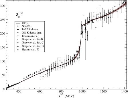
Figure 1: The new S0 wave unconstrained fit (UFD), where the dark band covers the uncertainties, versus the existing phase shift data from pipidata ; pipidata2 . Note that the $K\rightarrow 2\pi$ point has been excluded from the fit as explained in the text.

By defining $\delta_{M}=\delta(s_{M})$ and $\delta_{M}^{\prime}=d\delta(s_{M})/ds$, which are obtained from Eq. (6), and $k_{M}=|k_{2}(s_{M})|$, it is rather straightforward to impose continuity and a continuous derivative for the phase shift at $s_{M}$, to find:

$$\delta_{0}^{(0)}(s)=\left\{\begin{array}[]{ll}\displaystyle{d_{0}\left(1-\frac{|k_{2}|}{k_{M}}\right)^{2}+\delta_{M}\,\frac{|k_{2}|}{k_{M}}\left(2-\frac{|k_{2}|}{k_{M}}\right)+|k_{2}|(k_{M}-|k_{2}|)\left(8\delta_{M}^{\prime}+c\frac{(k_{M}-|k_{2}|)}{M_{K}^{3}}\right)},&(0.85\,{\rm GeV})^{2}<s<4M_{K}^{2},\\ \\ \displaystyle{d_{0}+B\frac{k_{2}^{2}}{M_{K}^{2}}+C\frac{k_{2}^{4}}{M_{K}^{4}}+D\,\theta(s-4M_{\eta}^{2})\frac{k_{3}^{2}}{M_{\eta}^{2}}},&4M_{K}^{2}<s<(1.42{\mbox{GeV}\,})^{2}.\end{array}\right.$$ (10)

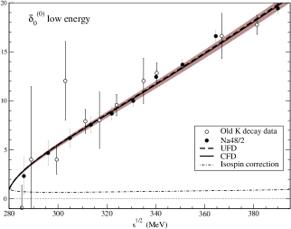
Figure 2: The new S0 wave unconstrained fit (UFD), where the dark band covers the uncertainties, versus the “old” phase shift data from $K_{\ell 4}$ decays Rosselet:1976pu together with the final NA48/2 results, which supersedes the data from the same experiment Batley:2007zz that we used in KPY08. We are also showing the isospin violation correction Colangelo:2008sm , which has been included in the data shown here. Finally, we show the results of the CFD parametrization to be explained in Sect. V, which is almost indistinguishable from the UFD curve.

As previously commented, with the exception of the $K\rightarrow 2\pi$ datum, the inclusion of isospin corrections to $K_{\ell 4}$ data explained above, and our use of the final NA48/2 results ULTIMONA48 , our treatment and selection of data for the phase is exactly the same one followed in the previous works Kaminski:2006yv and Yndurain:2007qm , so we will not repeat them here. In Table 4 of the Appendix, we provide the values for the $d_{0},c,B,C$ and $D$ parameters resulting from the unconstrained fit to those data. In Fig. 1 we show the resulting phase from the unconstrained data fit to the S0 wave phase shift up to 1420 MeV, and in Fig. 2 we show the low energy region in detail, including the isospin violation correction Colangelo:2008sm that we have subtracted from all the $K_{\ell 4}$ data. Note that this correction amounts to slightly less than 1 degree in the region from threshold to 400 MeV, which is not much at high energies, but very relevant close to threshold.

In Fig. 3 we show a comparison of the phase shift resulting from the new UFD with the improved matching versus the one obtained in KPY08. The changes at low energy are due to the update on the $K_{\ell 4}$ data and their isospin corrections, together with the fact that we now discard the $K\rightarrow 2\pi$ datum. The bump in the 500 to 800 MeV region observed in KPY08 has almost disappeared. Thus, the improvement on the data and its corrections reduces almost completely the disagreement of our UFD description with the phases in Bern —the line labeled CGL in the plot—although our central values are still larger in the 550-800 MeV region. Furthermore, as we will see later, for the constrained fits we are in an even better agreement with Bern . The changes above the matching point are sizable for the phase, mostly around the sharp phase increase usually associated with the $f_{0}(980)$ resonances, as can be seen in Fig. 3 where the central value for the new phase is compared with that in KPY08. Note the much smoother behavior in the matching region for the new UFD parametrization and the more dramatic $\bar{K}K$ threshold effect.

Concerning the S0 wave inelasticity, we approximate it to 1 up to the two-kaon threshold, and use the following parametrization above that energy:

$$\eta_{0}^{(0)}(s)=\exp\bigg{[}\frac{-k_{2}(s)}{s^{1/2}}\left(\tilde{\epsilon}_{1}+\tilde{\epsilon}_{2}\,\frac{k_{2}}{s^{1/2}}+\tilde{\epsilon}_{3}\,\frac{k_{2}^{2}}{s}\right)^{2}$$ (11)

$$-\tilde{\epsilon}_{4}\theta(s-4M_{\eta}^{2})\frac{k_{3}(s)}{s^{1/2}}\bigg{]},$$

for $4M_{K}^{2}<s<(1.42\,{\rm GeV})^{2}$. By neglecting the term proportional to the $\eta$ momentum, which is numerically very small as seen in the Appendix A.1, and by re-expanding the above equation in powers of $k_{2}/s^{1/2}$ up to third order, we recover the polynomial expression in KPY06, but the definition above ensures the $0\leq\eta_{0}^{(0)}\leq 1$ physical condition, whereas the simple polynomial in KPY06 did not.

For the inelasticity data, we follow again the same selection as in previous works of this series, but we do not include now the data from Kaminski et al. pipidata in the $\chi^{2}$ calculation; we only consider the 1973 data of Hyams et al. pipidata and Protopopescu et al. pipidata . The reason is that the main source of uncertainty is systematic, and if we include the large number of points of Kaminski et al. with their huge statistical errors, the outcome of the fit has much smaller errors than the original systematic uncertainties. By keeping only the other two sets, which are incompatible, we obtain a fit with a large $\chi^{2}/d.o.f.$, and by rescaling the uncertainties in the inelasticity parameters we mimic the dominant systematic uncertainties much better. Of course, our results are still in very good agreement with Kaminski et al. Was the systematic uncertainty not dominant, this would not be necessary. In Table 4 of the Appendix, we provide the values for the $\tilde{\epsilon}_{i}$ parameters, and in Fig. 4 we show the results of the unconstrained fit to the S0 wave inelasticity data up to 1420 MeV.

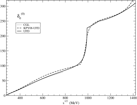
Figure 3: Fit to the S0 wave phase shift, with the improved continuous derivative matching (UFD, continuous line) versus the simpler one used in KPY08. We also show the phase predicted in Bern (CGL).

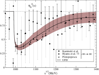
Figure 4: The new S0 inelasticity fit (UFD set) to the $\pi\pi\rightarrow\pi\pi$ scattering data of Hyams et al. (1973) and Protopopescu et al. As explained in the text, we do not fit the Kaminski et al. data pipidata although our fit is compatible with them. The dark band covers our uncertainties. For all data sets see Fig. 18.

Finally, let us remark that the inelasticity is the scattering parameter that suffers the biggest change with respect to the KPY08-KPY06 parametrization, as can be seen in Fig. 5. The new parametrization shows a big dip in the inelasticity between 1 and 1.1 GeV, whereas the KPY08 one does not. As already commented in PY05, this is a longstanding controversy (see, for instance Au:1986vs and references therein) between different sets of data coming from pure $\pi\pi\rightarrow\pi\pi$ scattering versus those coming from $\pi\pi\rightarrow\bar{K}K$ analysis. Actually, in PY05 (see Fig. 6 there) we considered both possibilities: we found that Forward Dispersion Relations favored the ”non-dip solution” very slightly, but we kept the ”dip-solution” in order to use the phase and inelasticity coming from the same experiment. In KPY06 we found a similar situation but since the K-matrix slightly preferred again the “non-dip solution”, this time we decided to use it. However, in terms of fulfillment, the difference is minute for FDRs, and even more so for standard Roy equations, since, as we have already commented and we will see in detail below, the uncertainties in the subtraction constants become so large above 500 MeV that we cannot use them to discard any of the two scenarios. The existing set of dispersion relations did not allow us to make a really conclusive statement about the inelasticity in the 1 GeV region.

One of the main results of this work is the derivation and use of once subtracted Roy-like dispersion relations, the GKPY equations presented in Sect. IV.4 below, which are more precise in the 1 GeV region and clearly favor the solution with a dip, thus helping to settle this dip versus non-dip controversy.

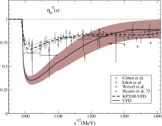
Figure 5: Fit to the S0 wave inelasticity (UFD) with the improved continuous derivative matching (continuous line) versus the simpler one used in KPY08 (dashed line). The dark band covers the uncertainties of the former, whereas the dotted curves enclose the uncertainties of the latter. Note that the drop in the inelasticity right above 1 GeV has become much deeper. In contrast to Fig. 4, we only show the data coming from $\pi\pi\rightarrow K\bar{K}$ and the $\pi\pi\rightarrow\pi\pi$ on which is based the KPY08 fit. For all data sets see Fig. 18.

IV Dispersion Relations and sum rules

From the theoretical side, $\pi\pi$ scattering is very special due to the strong constraints from isospin, crossing and chiral symmetries, but mostly from analyticity. The latter allows for a very rigorous dispersive integral formalism that relates the $\pi\pi$ amplitude at any energy with an integral over the whole energy range, increasing precision and providing information on the amplitude even at energies where data are poor, or in the complex plane.

Let us emphasize once more that the dispersive approach is model independent, since it makes the data parametrization irrelevant once it is included in the integral. The previous works Kaminski:2006qe ; Yndurain:2007qm of this series made use of two complementary dispersive approaches, Forward Dispersion Relations and Roy equations, that we briefly review next, before introducing the new set of once subtracted Roy-like equations.

IV.1 Forward Dispersion Relations (FDR)

They are calculated at $t=0$, so that the unknown large-$t$ behavior of the amplitude is not needed. There are two symmetric and one antisymmetric isospin combinations to cover the isospin basis. For further convenience we will write them as a difference $\Delta_{i}(s)$ that should vanish if the dispersion relation is satisfied exactly. In particular, the two symmetric ones, for $\pi^{0}\pi^{+}$ and $\pi^{0}\pi^{0}$, have one subtraction and imply the vanishing of

$$\Delta_{i}(s)\equiv{\mbox{Re}\,}F_{i}(s,0)-F_{i}(4M_{\pi}^{2},0)-\frac{s(s-4M^{2}_{\pi})}{\pi}\times$$

$$\hbox{P.P.}\int_{4M_{\pi}^{2}}^{\infty}\frac{(2s^{\prime}-4M^{2}_{\pi})\,{\mbox{Im}\,}F_{i}(s^{\prime},0)\,\hbox{d}\,s^{\prime}}{s^{\prime}(s^{\prime}-s)(s^{\prime}-4M_{\pi}^{2})(s^{\prime}+s-4M_{\pi}^{2})},\;$$ (12)

where $F_{i}$ stands for the $F_{0+}(s,t)$ or $F_{00}(s,t)$ amplitudes, and “P.P.” stands for the principal part of the integral. They are very precise, since all the integrand contributions are positive. The antisymmetric isospin combination $I_{t}=1$ does not require subtractions and implies the vanishing of the following difference:

$$\Delta_{(I_{t}=1)}(s)\equiv F^{(I_{t}=1)}(s,0)-\frac{2s-4M^{2}_{\pi}}{\pi}\times$$

$$\hbox{P.P.}\int_{4M^{2}_{\pi}}^{\infty}\hbox{d}\,s^{\prime}\,\frac{{\mbox{Im}\,}F^{(I_{t}=1)}(s^{\prime},0)}{(s^{\prime}-s)(s^{\prime}+s-4M^{2}_{\pi})}.$$

All FDRs are calculated up to $\sqrt{s}=1420$ MeV.

IV.2 Roy Equations

These are an infinite set of coupled equations Roy:1971tc , equivalent to non-forward dispersion relations plus $t-s$ crossing symmetry. They are well suited to study poles of resonances and scattering data, since they are written directly in terms of partial waves $t^{(I)}_{\ell}$ of definite isospin $I$ and angular momentum $\ell$. Remarkably, S. M. Roy managed to rewrite the complicated left cut contribution as a series of integrals over the physical region. In the original work of Roy and all applications until now, the convergence of the integrals was ensured by making two subtractions.

As we did with FDR, we will recast each one of the Roy Equations as the difference

$$\Delta_{\ell}^{(I)}(s)\equiv\mbox{Re }t_{\ell}^{(I)}(s)-ST_{\ell}^{I}(s)-DT_{\ell}^{I}(s)$$

$$-\sum_{I^{\prime}=0}^{2}\sum_{\ell^{\prime}=0}^{1}\mbox{P.P.}\int_{4M_{\pi}^{2}}^{s_{max}}ds^{\prime}K_{\ell\ell^{\prime}}^{II^{\prime}}(s,s^{\prime})\mbox{Im }t_{\ell^{\prime}}^{I^{\prime}}\!(s^{\prime}),$$ (14)

that should vanish when the equation is exactly satisfied. Roy equations provide as output the real part of partial waves below 1115 MeV. Although, in principle, one could consider output for waves up to higher $\ell$, in this work we are interest in results for $\ell=0,1$ only. Hence, we have separated those waves explicitly below $s_{max}$.

As it was done in KPY08, below $s^{1/2}_{max}=1420$ MeV, we consider the imaginary parts from all our $\ell\leq 4$ partial wave parametrizations as input. Above that energy, we take into account all waves together parametrized with Regge theory—see Appendix A.8. The $K_{\ell\ell^{\prime}}^{II^{\prime}}(s,s^{\prime})$ are known kernels, and thus we will refer to the integral terms as “kernel terms” or $KT(s)$. The “driving terms”, $DT_{\ell}^{I}(s)$, have the same structure as the kernel terms, but their input contains both the contribution from $\ell=2,3$ partial waves up to $s_{max}^{1/2}=1420$ MeV, and the Regge parametrizations above. We have explicitly checked that the $\ell=4$ contribution below $s_{max}$ is irrelevant, so that we will refer just to waves up to $\ell=3$. Finally, the so-called subtraction terms are given by:

$$ST_{\ell}^{I}(s)= a_{0}^{0}\delta_{I0}\delta_{\ell 0}+a_{0}^{2}\delta_{I2}\delta_{\ell 0}+\frac{s-4M_{\pi}^{2}}{12M_{\pi}^{2}}\times$$ (15)

$$(2a_{0}^{0}-5a_{0}^{2})(\delta_{I0}\delta_{\ell 0}+\frac{1}{6}\delta_{I1}\delta_{\ell 1}-\frac{1}{2}\delta_{I2}\delta_{\ell 0}).$$

It is very relevant to remark once more that these equations have two subtractions, as can be seen by the presence of the term proportional to $(s-4M_{\pi}^{2})(2a_{0}^{0}-5a_{0}^{2})$. This strong energy dependence of $ST(s)$ makes these twice subtracted Roy Equations very suitable for low energy studies, and even more so when complemented with theoretical predictions of the scattering lengths coming from ChPT Bern .

Roy Equations are valid up to $\sqrt{s}\leq 8M_{\pi}\simeq 1120$ MeV. However, we will see that the uncertainties in the scattering lengths, when propagated to high energies, become too large above roughly 450 MeV, due to the term proportional to $s$. For this reason, in KPY08 it did not make sense to deal with the complications of a precise description around $\bar{K}K$ threshold and thus we implemented them up to $2M_{K}$. One of the main novelties of the present work is that, since the once-subtracted Roy-like equations explained below will have much smaller uncertainties in the $\bar{K}K$ threshold region, we have now implemented these new equations, together with the standard Roy equations, up to 1115 MeV.

IV.3 Two Sum Rules

Apart from FDRs and Roy equations, two sum rules that relate high energy (Regge) parameters for $t\neq 0$ to low energy P and D waves, have been considered throughout previous works.

The first sum rule (PY05) is nothing but the vanishing of the following difference

$$I\equiv\int_{4M^{2}_{\pi}}^{\infty}\!\!\hbox{d}\,\!s\,\frac{{\mbox{Im}\,}F^{(I_{t}=1)}(s,4M^{2}_{\pi})-{\mbox{Im}\,}F^{(I_{t}=1)}(s,0)}{s^{2}}$$

$$\!\!\!\!\!-\int_{4M^{2}_{\pi}}^{\infty}\hbox{d}\,\!s\,\frac{8M^{2}_{\pi}[s-2M^{2}_{\pi}]\,{\mbox{Im}\,}F^{(I_{s}=1)}(s,0)}{s^{2}(s-4M^{2}_{\pi})^{2}},\quad$$ (16)

where the contributions of the S waves cancel and only the P and D waves contribute (we also include F and G waves, but they are negligible). At high energy, the integrals are dominated by the rho reggeon exchange.

The second sum rule we consider is given in Eqs. (B.6) and (B.7) of the second reference in Bern , which requires the vanishing of

$$J\equiv\int_{4M^{2}_{\pi}}^{\infty}\hbox{d}\,s\,\Bigg{\{}\frac{4{\mbox{Im}\,}F^{\prime(0)}(s,0)-10{\mbox{Im}\,}F^{\prime(2)}(s,0)}{s^{2}(s-4M^{2}_{\pi})^{2}}$$

$$-6(3s-4m^{2}_{\pi})\,\frac{{\mbox{Im}\,}F^{\prime(1)}(s,0)-{\mbox{Im}\,}F^{(1)}(s,0)}{s^{2}(s-4M^{2}_{\pi})^{3}}\Bigg{\}}.\quad$$ (17)

Here, $F^{\prime(I)}(s,t)\equiv\partial F^{(I)}(s,t)/\partial\cos\theta$. At high energy, the integral is dominated by isospin zero Regge trajectories.

IV.4 GKPY Equations

The main novelty of this work is that we present and use a new set of Roy-like dispersion relations for $\pi\pi$ scattering amplitudes. For brevity, we will call them GKPY equations, as we have already done when presenting some partial and preliminary results in several conferences MonteCarlo ; Kaminski:2008rh . In brief, their derivation follows the same steps as for Roy equations, starting from fixed $t$ dispersion relations for a complete isospin basis, that S. M. Roy subtracted twice to ensure that the integrals converged when extended to infinity. However, by using the complete set of isospin amplitudes $F_{00}$, $F_{0+}$ and $F^{(I_{t}=1)}$, it is easy to see that one subtraction is enough. Actually, the two first amplitudes are $s-u$ symmetric and the contributions from the $s$ and $u$ channels, that would be divergent by themselves alone, cancel when considered simultaneously. The $F^{(I_{t}=1)}$ amplitude is dominated by the rho Regge exchange and neither the left nor the right cut are divergent with one subtraction. We provide the detailed derivation in Appendix B, which leads to the vanishing of the following difference:

$$\Delta_{\ell}^{GKPY\,(I)}\equiv\mbox{Re }t_{\ell}^{(I)}(s)-\overline{ST}_{\ell}^{I}-\overline{DT}^{I}_{\ell}(s)$$

$$-\sum_{I^{\prime}=0}^{2}\sum_{\ell^{\prime}=0}^{1}\mbox{P.P.}\int_{4M_{\pi}^{2}}^{s_{max}}ds^{\prime}\overline{K}_{\ell\ell^{\prime}}^{II^{\prime}}(s^{\prime},s)\mbox{Im }t_{\ell^{\prime}}^{(I^{\prime})}(s^{\prime}).$$ (18)

The subtraction terms $\overline{ST}_{\ell}^{I}$ are linear combinations of scattering lengths $a_{0}^{I}$, and can be found in Appendix B. A very relevant observation for this work is that, in contrast to the standard Roy Equations, the subtraction terms in GKPY do not depend on $s$.

The integral and driving terms $\overline{DT}_{\ell}^{I}(s)$ in Eq. (18) are analogous to the kernel and driving terms in Roy equations, but the integrals contain the $\overline{K}_{\ell\ell^{\prime}}^{II^{\prime}}$ kernels, instead of the $K_{\ell\ell^{\prime}}^{II^{\prime}}$. The explicit expressions for $\overline{K}_{\ell\ell^{\prime}}^{II^{\prime}}$ are lengthy and we provide them in Appendix C. Note that, as the once subtracted GKPY equations have kernel terms that behave as $\sim 1/s^{2}$ at higher energies, instead of the $\sim 1/s^{3}$ behavior in Roy equations, the weight of the high energy region is larger. Nevertheless, the contribution to the driving terms coming from energies above 1.42 GeV is generically smaller than the contribution coming from the D and F waves below 1.42 GeV, which means that their influence is still under control.

IV.5 Roy versus GKPY Equations

Fig. 6 presents a decomposition of Roy equations for the S0, P and S2 waves into four parts: the “in” part, that represents what our parametrizations give for ${\mbox{Re}\,}t_{\ell}^{(I)}$, the subtracting terms $ST(s)$, the kernel terms $KT(s)$ and the driving terms $DT(s)$. Note that, for these equations to be satisfied exactly, the first contribution should equal the sum of the other three. The numerical calculations have been performed by taking the UFD amplitudes described in the previous Sections as input. For illustration, we have drawn as a gray area the region that violates the unitarity bound $|{\rm Re}\,t|\leq\eta s^{1/2}/4k$, (note that $\eta=1$ in the elastic region). For comparison, we present in Fig. 7 the same decompositions for the GKPY equations. Note the very different scales on both sets of Figures.

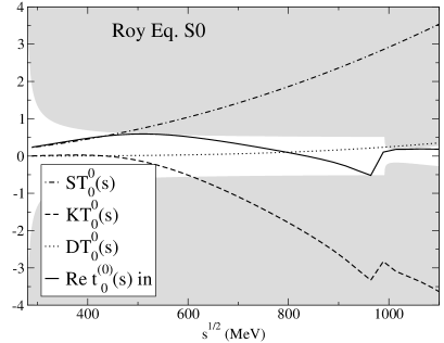
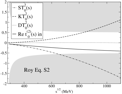
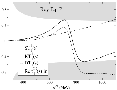
Figure 6: Using the UFD set as input, we show the decomposition of Roy equations into the subtracting term $ST$, kernel term $KT$, and driving term $DT$ for the S0, P and S2 waves. Note the different scales used on each plot.

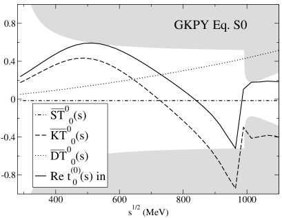
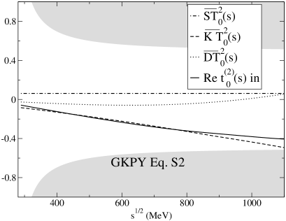
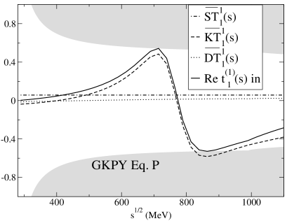
Figure 7: Using the UFD set as input, we show the decomposition of GKPY equations into the subtracting term $\overline{ST}$, kernel term $\overline{KT}$, and driving term $\overline{DT}$ for the S0, P and S2 waves. Note the different scales used here and in Fig. 6.

As can be seen in Fig. 6, the $ST(s)$ and $KT(s)$ terms in Roy equations become huge at higher energies and suffer a large cancellation against each other. This cancellation is particularly strong for the S0 wave, where, for a sufficiently large energy, both terms are much larger than the unitarity bound. For instance, they are larger by roughly a factor of four at 750 MeV, and of eight at 1100 MeV.

In contrast, as seen in Fig. 7 for the GKPY equations, Eq. (18), the $\overline{ST}$ terms are constant, and in fact much smaller than the $\overline{KT}(s)$ terms, which are clearly the dominant ones. Therefore, no big cancellations between any two terms are needed in order to reconstruct the total real part of the amplitude. Moreover, we have checked that the high energy part, which has been parametrized by means of Regge theory, corresponds to somewhat less than half of the total $\overline{DT}(s)$ contribution. Therefore, although the $\overline{DT}(s)$ terms in the GKPY equations are larger than in Roy equations due to the fact that there is one subtraction less, the contribution coming from the amplitudes above 1420 MeV is still small compared with the dominant term $KT(s)$. Thus, the high energy behavior is still well under control.

Note that, to keep the plots clear, we have only provided central values for the moment. In the next section we will provide the total uncertainties (the uncertainties of each separated contribution were presented in a conference Kaminski:2008rh using a very preliminary UFD set). For our purposes it is enough to remark that uncertainties follow a similar pattern to these central values. In particular, the $ST(s)$ term in Roy equations for scalar waves has a large uncertainty due to the poor experimental knowledge of the $a^{2}_{0}$ scattering length, that becomes larger and larger, proportionally to $s$, as the energy grows, becoming dominant above roughly 450 MeV. In contrast, since the GKPY $\overline{ST}$ term is constant and there are no large cancellations, the resulting GKPY equations have a much smaller uncertainty in that region. Actually, the errors for the GKPY equations in the three waves come almost completely from the $\overline{KT}(s)$ terms. At low energies, the effect is reversed and Roy equations provide a much more stringent constraint than GKPY. Therefore, and as we will show next, they become complementary ways of checking our data parametrizations at different energies.

IV.6 Consistency check of Unconstrained Fits

In order to provide a consistency measure for our parametrizations with respect to the dispersive relations and sum rules presented in the previous sections, we will make use (as we did in previous works) of a quantity similar to an averaged $\chi^{2}/(d.o.f.)$ distribution. In particular, we can consider that a dispersion relation $i$ is well satisfied at a point $s_{n}$ if the difference $\Delta_{i}$, defined in Eqs. (12), (IV.1), (14) and (18), is smaller than its uncertainty $\delta\Delta_{i}$. Thus, when the average discrepancy verifies

$$\bar{d}_{i}^{2}\equiv\frac{1}{\hbox{number of points}}\sum_{n}\left(\frac{\Delta_{i}(s_{n})}{\delta\Delta_{i}(s_{n})}\right)^{2}\leq 1,$$ (19)

we consider that the corresponding dispersion relation is well satisfied within uncertainties in the energy region spanned by the points $s_{n}$. In practice, the values of $s_{n}^{1/2}$ are taken at intervals of 25 MeV between threshold and the maximum energy where we study each dispersion relation (1420 MeV for FDR and 1115 MeV for Roy and GKPY equations). In addition, we have added a point below threshold at $s=2M_{\pi}^{2}$ for the $F_{00}$ and $F_{0+}$ FDRs.

Similarly, we define discrepancies for the sum rules in Eqs. (16) and (17), as follows:

$$\bar{d}^{2}_{I}=\left(\frac{I}{\delta I}\right)^{2},\quad\bar{d}^{2}_{J}=\left(\frac{J}{\delta J}\right)^{2}.$$ (20)

In order to calculate the uncertainties $\delta\Delta_{i}(s_{n})$, $\delta I$, $\delta J$, we have followed two approaches: On the one hand we have simply added in quadrature the effect of varying each parameter independently in our parametrizations from $p_{i}$ to $p_{i}\pm\delta p_{i}$. The errors are symmetric since, in order to be conservative, we have always taken the largest variation as the final error when changing the sign of $\delta p_{i}$. This is rather simple but does not take their correlations into account. On the other hand, we have also estimated the uncertainties using a Monte Carlo Gaussian sampling MonteCarlo of all CFD parameters (within 6 standard deviations). The uncertainties are then slightly asymmetric, corresponding to the independent left and right widths of the generated distribution for $10^{5}$ events. This is, of course, much more time consuming, although in this way we can keep part of the correlations in the results. However, we have checked that both methods yield very similar results, because the errors coming from each individual parameter are small and the number of parameters is large. The difference between using one method or another is almost negligible MonteCarlo and thus, for simplicity, we are providing numbers and figures with the first one, that would be much easier to reproduce should someone use our parametrizations.

In Table 1 we show the averaged squared discrepancies $\bar{d}_{i}^{2}$ that result when we use the UFD set described in Sects. II and III. We are showing these discrepancies up to two different energy regions, 932 MeV and 1420 MeV for FDRs, and up to 992 MeV and 11115 MeV for both Roy and GKPY equations (note that we have kept the same definition of energy regions as in KPY08, so that we can compare easily with the results obtained there). Let us remark that these discrepancies are “squared distances”, similar to a $\chi^{2}$, and so we will abuse the language and talk about average “standard deviations”, which correspond to the square root of $\bar{d}_{i}^{2}$. Still, one has to keep in mind that these dispersion relations have not been fitted yet.

Let us first concentrate in the low energy part below 932 MeV or 992 MeV. We can observe that FDRs are reasonably well satisfied: discrepancies are never beyond 1.3 standard deviations. Roy equations are also well satisfied, with a discrepancy below 1.2 standard deviations. However, the GKPY equations are much more demanding: The UFD set satisfies the S2 wave equation fairly well, but it does not satisfy the S0 and P wave relations so well. Still, no dispersion relation lies beyond 1.6 standard deviations. This is not too bad, given the fact that we have not fitted the dispersion relations, but there is clear room for improvement. Let us recall that this is just how experimental data satisfy these constraints, there is no theory on the UFD set.

$\qquad\bar{d}_{i}^{2}$	new UFD	old UFD	new UFD	old UFD
FDRs	$s^{1/2}\leq 932\,$MeV		$s^{1/2}\leq 1420\,$MeV
$\pi^{0}\pi^{0}$	0.31	0.12	2.13	0.29
$\pi^{+}\pi^{0}$	1.03	0.84	1.11	0.86
$I_{t=1}$	1.62	0.66	2.69	1.87
Roy Eqs.	$s^{1/2}\leq 992\,$MeV		$s^{1/2}\leq 1100\,$MeV
S0	0.64	0.54	0.56	0.47
S2	1.35	1.63	1.37	1.68
P	0.79	0.74	0.69	0.65
GKPY Eqs.	$s^{1/2}\leq 992\,$MeV		$s^{1/2}\leq 1100\,$MeV
S0	1.78	5.0	2.42	8.6
S2	1.19	0.49	1.14	0.58
P	2.44	3.1	2.13	2.7
Average	1.24	1.46	1.58	1.97

Table 1: Average discrepancies $\bar{d}_{i}^{2}$ of the unconstrained data fits (UFD set) for each dispersion relation. We compare the results of the parametrization obtained in this work (new UFD) with those in KPY08 (old UFD set). The huge discrepancies seen in KPY08 for GKPY equations all come from energies above $\sim 500\,{\mbox{MeV}\,}$. This is the main reason to improve our unconstrained S0 fit as explained in Sect. III.3.

If we now also include the region above 932 MeV for FDRs or above 992 MeV for Roy and GKPY equations, we find that the agreement deteriorates considerably: four relations lie between 1.4 and 1.65 average standard deviations, but not beyond that. Fortunately we will get much better fulfillment of dispersion relations in all regions by allowing for a small variation of the parameters in the constrained fits to be discussed below.

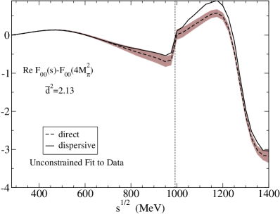
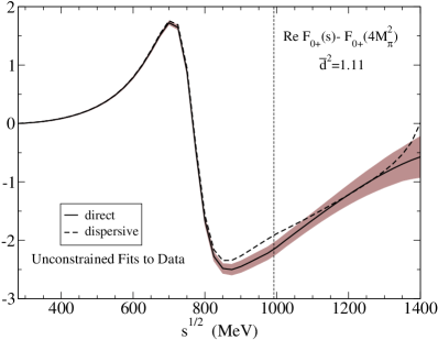
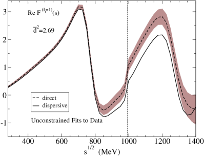
Figure 8: Results for Forward Dispersion Relations. Dashed lines: real part, evaluated directly with the UFD parametrizations. Continuous lines: the result of the dispersive integrals. The dark bands cover the uncertainties in the difference between both. From top to bottom: (a) the $\pi^{0}\pi^{0}$ FDR, (b) the $\pi^{0}\pi^{+}$ FDR, (c) the FDR for $I_{t}=1$ scattering. The dotted vertial line stands at the $\bar{K}K$ threshold.

Let us also remark that the two sum rules, Eqs. (16) and (17), are satisfied within 1.9 and 0.3 standard deviations. Even for the first one, this is still a fair agreement, because, in practice, both of them correspond to a one-order of magnitude cancellation between the low and high energy contributions to the sum rules, which, in these UFD set are determined from uncorrelated data fits.

Also in Table 1 we show the average discrepancies for the old UFD set in KPY08. With regard to FDRs and Roy equations, it is evident that the new UFD fit is doing worse than the one in KPY08. Nevertheless, one should keep in mind that the new S0 wave has reduced its uncertainty at low energies by somewhat more than 10%, because the published NA48/2 data are more precise and also because we are discarding the controversial $K\rightarrow 2\pi$ datum. For that reason, one would have expected the averaged squared discrepancies to look now bigger by as much as 20 or 30% whenever the S0 wave contributes significantly to the dispersion relation. With this correction in mind, the deterioration is not so significant. Nevertheless, we want to insist that this is basically due to the new results of NA48/2 and our getting rid of the $K\rightarrow 2\pi$ datum. The data have changed.

Why do we then claim to have improved the S0 wave in this work? The answer comes from GKPY equations, which, as we already explained, are much more precise than Roy equations above roughly 450 MeV for the S0 wave, given the present experimental input. It is clear that the KPY08 UFD parametrization satisfies the S0 GKPY equation very poorly at any energy and is not satisfying the low energy P GKPY equation very well. For that reason, we have improved the matching and the data selection, so that our new UFD parametrization, that will be our starting point for the constrained fits, satisfies GKPY equations much better without spoiling FDR and Roy equations. The improvement due to the new unconstrained S0 wave fit is obvious from Table 1, particularly in the S0 GKPY equation. Up to 1100 MeV, the old UFD set from KPY08 had an averaged squared discrepancy of 8.6, whereas the new UFD set has 2.42. This huge improvement on the S0 wave has been compensated by some deterioration in other relations at high energy, so that the averaged discrepancy up to high energies is reduced only from 1.97 to 1.58. Note that the change in the inelasticity parameter, that now shows a much bigger dip in the 1000 to 1100 MeV region, as shown in Fig. 5, plays a relevant role in this dramatic improvement. This dip structure is thus favored by the GKPY equations, something that could not be seen with standard Roy equations since their uncertainties in that region are huge. We will discuss this in detail in Sect. VII.2. At low energies, the average squared discrepancy has been reduced very little, from 1.46 down to 1.24. Of course, let us remark once again that our uncertainties are now 10-15% smaller in the S0 wave at low energies, so that the improvement is actually bigger than it seems just from the numbers in the table.

Let us mention here that the inclusion of the new terms parametrizing a crude dependence on the $\eta$ momentum above $\eta\eta$ threshold, help reducing the average squared distances by 6%, namely, from 1.68 to 1.58. In particular, the averaged squared discrepancies $\bar{d}_{i}^{2}$ for the S0 GKPY equation decrease from 3.02 to 2.42 and for the $F_{00}$ FDR equation from 2.35 to 2.13.

Up to now, we have studied the overall uncertainties, but in Fig. 8 we show to what extent FDRs are satisfied by the UFD set, as a function of energy. Of course, the best fulfillment is found at lower energies. In Fig. 9 we show how the usual, twice subtracted Roy equations are satisfied by the UFD set. Here, as we did in Sect. IV.5, we denote by “in” what our parametrizations give for ${\mbox{Re}\,}t_{\ell}^{(I)}$, whereas we denote by “out” the result of the dispersive representation from Roy equations, namely, the subtraction constant terms, plus the kernel terms, plus the driving terms in Eq. (14). Finally, in Fig. 10 we show how the new, once subtracted, GKPY equations are satisfied by the UFD set. We follow the same “in” and “out” notation as for Roy equations.

Comparing Fig. 9 with Fig. 10, it is clear that, given the present experimental input, the uncertainty band for GKPY equations is much smaller than that for Roy equations above 450 MeV, whereas the opposite occurs at lower energies. Therefore, as we have emphasized repeatedly, the new GKPY equations represent a much stronger constraint in the intermediate energy region than standard Roy equations.

In summary, with the new S0 unconstrained fit, all dispersion relations are satisfied in the different energy regions within less than 1.6 standard deviations in the low energy regime, and 1.7 including the intermediate energies. This is a fairly reasonable fulfillment, given the fact that the information about analyticity has not been included as a constraint in the UFD description. Nevertheless, it is obvious that there is room for improvement, which is what we will do by obtaining constrained data fits in the next section.

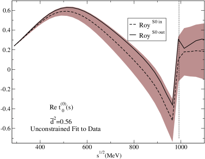
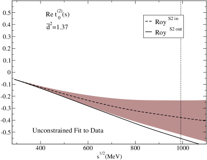
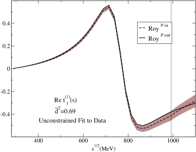
Figure 9: Results for Roy Equations. Dashed lines (“in”): real part, evaluated directly with the UFD parametrizations. Continuous lines (“out”): the result of the dispersive representation. The gray bands cover the uncertainties in the difference between both. From top to bottom: (a) S0 wave, (b) S2 wave, (c) P wave. The dotted vertial line stands at the $\bar{K}K$ threshold.

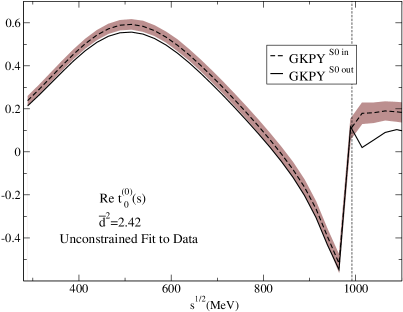
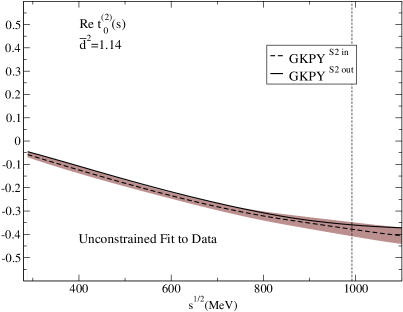
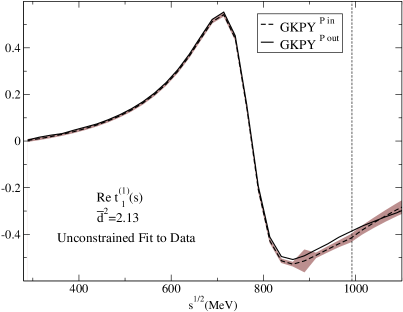
Figure 10: Results for GKPY equations. Dashed lines (“in”): real part, evaluated directly with the UFD parametrizations. Continuous lines (“out”): the result of the dispersive representation. The gray bands cover the uncertainties in the difference between both. From top to bottom: (a) S0 wave, (b) S2 wave, (c) P wave. Note how these uncertainties are much smaller above 450 MeV than those from standard Roy equations shown in Fig. 9. The dotted vertial line stands at the $\bar{K}K$ threshold.

V Fits to Data Constrained by Dispersion Relations

In previous works (PY05, KPY08) we had improved the consistency of our description of $\pi\pi$ scattering amplitudes by imposing FDR and Roy equations fulfillment within uncertainties. As we have just seen in the previous section, the GKPY equations provide a much more stringent constraint in the intermediate energy region than standard Roy equations and thus it now makes sense to impose the new GKPY equations as an additional constraint in a new set of Constrained Fits to Data (CFD set).

V.1 Minimization procedure

Our goal is then to obtain a fit to data, by changing the UFD parametrizations slightly, that fulfills each dispersion relation within errors. As we did in Kaminski:2006qe , we will now use the average discrepancies $\bar{d}_{i}^{2}$, defined in Eqs. (19) and (20), to obtain these constrained fits, by minimizing:

$$\sum_{i}W^{2}_{i}\bar{d}_{i}^{2}+\bar{d}^{2}_{I}+\bar{d}^{2}_{J}+\sum_{k}\left(\frac{p_{k}-p_{k}^{\rm exp}}{\delta p_{k}}\right)^{2},$$ (21)

where $i$ runs over the three FDRs, the three Roy and the three GKPY equations. Here, we denote by $p_{k}^{exp}$ all the parameters of the UFD parametrizations for each wave or Regge trajectory. In this way we force the previous data parametrizations to satisfy dispersion relations and sum rules within uncertainties. In KPY06 and KPY08 a common weight of $W_{i}^{2}\sim 9$ was estimated from the typical number of degrees of freedom needed to describe the shapes of the output. This value ensured that every single dispersion relation was fairly well described by the KPY08 constrained data fits up to the matching energy used in that work, namely, 932 MeV.

However we are now considering partial waves up to 1115 MeV. For most waves, this extension does not alter significantly their shape and $W_{i}=3$ is still a good weight. Nevertheless, we have less points in the region above 932 MeV and if we want the fit to give not just a good average $\bar{d}_{i}^{2}$, but also a good description for each wave, some of these waves need further weight on the high energy region, in particular if their UFD $\bar{d}_{i}^{2}$ was larger than 2. For this purpose, we have increased $W_{i}$ up to 3.5 for the high energy parts of the $F_{00}$, $F^{(I_{t}=1)}$, as well as 4.2 for the GKPY P wave in the whole energy region. Finally, we have increased $W_{i}$ up to 7 for the high energy part of the S0 GKPY equation. The latter was to be expected, since in this region there is a lot more of structure, both in the phase and inelasticity, due to the presence of the $f_{0}(980)$. These values are not arbitrary, since they have been obtained by increasing each $W_{i}$ gradually, starting from 3, until the $\bar{d}_{i}^{2}$ are below or very close to one uniformly throughout the whole energy range, for all dispersion relations obtained from the constrained fit. This uniformity is very relevant to avoid dispersive constraints being badly satisfied in some small energy region despite the averaged $\bar{d}^{2}_{i}$ still remaining below 1.

Before proceeding further, let us recall that, strictly speaking, the quantity that we minimize in Eq. (21) is not a $\chi^{2}$, but that each individual $\bar{d}_{i}^{2}$ is a measure of how well each dispersion relation is satisfied.

V.2 Variation of the S2 Adler zero

As we have seen in Section III.3, in the parametrization of each scalar wave we explicitly factorized a zero in the subthreshold region. These are the Adler zeros required by chiral symmetry constraints Adler:1964um . Actually, we fixed them to $\sqrt{s_{A}^{S0}}\equiv\sqrt{M_{\pi}^{2}/2}\simeq 99\,$MeV and $\sqrt{s_{A}^{S2}}\equiv\sqrt{2M_{\pi}^{2}}\simeq 197\,$MeV, which are their current algebra values (leading order ChPT). Of course, once these UFD parametrizations are used inside the S0 and S2 Roy or GKPY equations we can also obtain the dispersive result for the S0 and S2 Adler zeros, that we provide in Table 2.

In order to determine the positions of Adler zeros better when making constrained fits in KPY08, we allowed them to change within the dispersive uncertainties obtained from the UFD set. However, in this work we will not insist on $z_{0}/\sqrt{2}$ reproducing the S0 wave Adler zero very precisely. The reason is that, as we see in Table 2, the uncertainties in $\sqrt{s_{A}^{S0}}$ obtained either from Roy or GKPY equations are huge, and setting $z_{0}$ free introduces a spurious and extremely correlated source of error. In addition, in KPY08, the $z_{0}$ central value moved in the wrong direction . In addition, as already explained in Sect. III.3, the S0 wave Adler zero lies close to the border of the conformal circle, i.e., $w(s_{A}^{S0})\simeq-1$, where the conformal expansion coverges very slowly. We simply have to accept that our S0 wave conformal expansion is not very accurate around the Adler zero. Of course, this is irrelevant for the integrals in the physical region and has a negligible influence in the set of constrained fits we will obtain next.

	Roy Eqs.	GKPY Eqs.	Roy Eqs.	GKPY Eqs.
	with UFD	with UFD	with CFD	with CFD
$\sqrt{s_{A}^{S0}}$	$112\pm 24$	$120\pm 30$	$83\pm 32$	$85\pm 34$
$\sqrt{s_{A}^{S2}}$	$189\pm 11$	$200\pm 6$	$200\pm 10$	$201\pm 5$

Table 2: Adler zero positions $\sqrt{s_{A}}$, in MeV, for the S0 and S2 waves, obtained from Roy or GKPY equations using either the parametrizations form the UFD or CFD sets.

In contrast, the S2 Adler zero obtained from the dispersive representation moves very little from its current algebra value and its uncertainty is rather small. The reason for this difference in uncertainties is, for a good part, that the S0 wave Adler zero lies very close to the left cut, whereas the S2 Adler zero is not so far from threshold and is quite well determined when data is used as input of either Roy or, even better, GKPY equations. For that reason, we still allow the S2 Adler zero to vary when making the constrained fits, using as a starting point the weighted average of the values obtained from the UFD set inside Roy and GKPY equations, namely, $\sqrt{s_{A}^{S2}}=197.7\pm 5.1\,{\mbox{MeV}\,}$.

V.3 The Constrained Fits to Data (CFD)

The resulting parameters for the CFD are gathered in the tables of the Appendix A. It is reassuring to observe that, except for the S0 wave at intermediate energies, the values of the parameters do not change much from the UFD to the CFD sets, as could be expected, since, as we saw in Table 1, the UFD fulfillment of dispersive constraints only needed some improvement, but not a radical change. In particular, the GKPY equation for the S0 wave is very well satisfied in the CFD at the expense of an average change of 0.82 standard deviations in the high energy parameters and almost no change in the low energy ones. Certainly, most of this change is concentrated in the parameters $c$ and $\tilde{\epsilon}_{1}$ in Eqs. (10) and (III.3). We will discuss below that the resulting phase after this change still describes the phase shift and inelasticity data fairly well, but tends to make the $f_{0}(980)$ somewhat wider. The D2 wave is the one that deviates most from its unconstrained parametrization, but its parameters are, on average, within 1.4 standard deviations of their UFD value. This could be expected, as was already commented in our previous works Pelaez:2004vs ; Kaminski:2006qe , since, together with the S0 at high energy, it is probably the one where data has the worst quality. The parameters of the other waves, or those of the Regge parametrizations, do not deviate—on the average—beyond 0.6 standard deviations from their UFD values. In Table 11 in Appendix D we provide the S0, P and S2 phase-shifts that result from using the CFD set inside the dispersive representation.

FDRs	$s^{1/2}\leq 932\,$MeV	$s^{1/2}\leq 1420\,$MeV
$\pi^{0}\pi^{0}$	0.32	0.51
$\pi^{+}\pi^{0}$	0.33	0.43
$I_{t=1}$	0.06	0.25
Roy Eqs.	$s^{1/2}\leq 992\,$MeV	$s^{1/2}\leq 1100\,$MeV
S0	0.02	0.04
S2	0.21	0.26
P	0.04	0.12
GKPY Eqs.	$s^{1/2}\leq 992\,$MeV	$s^{1/2}\leq 1100\,$MeV
S0	0.23	0.24
S2	0.12	0.11
P	0.68	0.60
Average	0.22	0.28

Table 3: Average discrepancies $\bar{d}_{i}^{2}$ of the Constrained Fits to Data (CFD) for each dispersion relation.

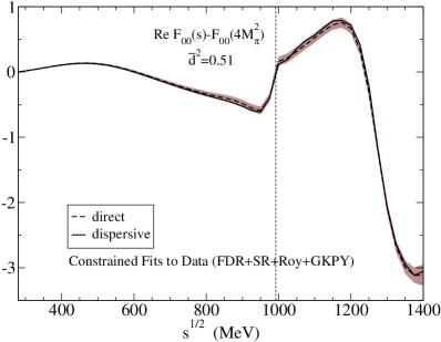
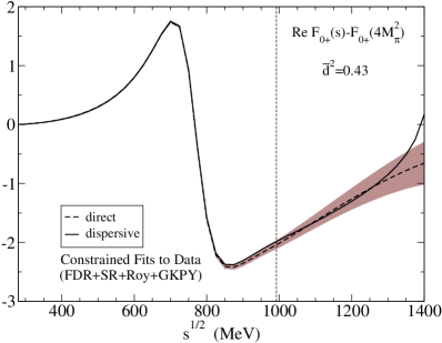
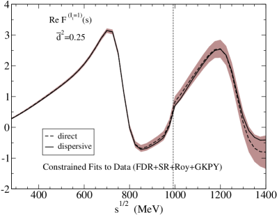
Figure 11: Results for forward dispersion relations. Dashed lines: real part, evaluated directly with the CFD parametrizations. Continuous lines: the result of the dispersive integrals. The dark bands cover the uncertainties in the difference between both. From top to bottom: (a) the $\pi^{0}\pi^{0}$ FDR, (b) the $\pi^{0}\pi^{+}$ FDR, (c) the FDR for $I_{t}=1$ scattering.

In Table 3 we list the averaged discrepancies that result when we use the constrained fits (CFD) inside the dispersion relations. Let us remark that all discrepancies are now below one, and very similar both for the low energy region and also when including the high energy region. This shows a remarkable average consistency and homogeneity for this new set of data parametrizations. Let us recall that we only constrain our fits to satisfy dispersion relations up to 1420 MeV for FDR and 1115 MeV for Roy and GKPY equations. Consequently, we expect the dispersive representation to be somewhat worse satisfied in the region near the maximum energy under consideration. This is indeed observed since the average squared discrepancies are somewhat smaller below 1 GeV than up to the maximum energy, where we usually find the point satisfying the dispersion relations worse.

Furthermore, as already commented, the updated selection and treatment of the S0 wave data has decreased the S0 wave uncertainties by roughly 10 to 15%. This means that the consistency shown by the average discrepancies in Table 3 is even better than it looks when comparing with similar results given in KPY08 for FDR and Roy equations, since we are getting a very good consistency with slightly smaller uncertainties.

As we did for the UFD set, we now show in Figs. 11, 12 and 13, how well the CFD set satisfies FDR, Roy and GKPY equations respectively. The improvement in the consistency of the CFD set over the UFD is evident by comparing these plots with their UFD counterparts in Figs. 8, 9 and 10.

Finally, the two sum rules in Eqs. (16) and (17) are also remarkably well satisfied, within 0.93 and 0.1 standard deviations, respectively. In particular, the 1.9 standard deviations for the sum rule in Eq. (17) using the UFD set are reduced dramatically, and this implies now a two orders of magnitude cancellation between the low and high energy contributions.

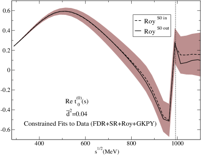
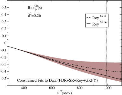
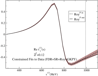
Figure 12: Results for Roy equations. Dashed lines (“in”): real part, evaluated directly with the CFD parametrizations. Continuous lines (“out”): the result of the dispersive representation. The gray bands cover the uncertainties in the difference between both. From top to bottom: (a) S0 wave, (b) S2 wave, (c) P wave.

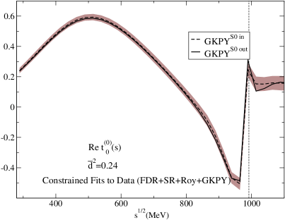
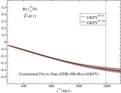
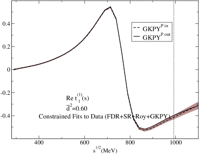
Figure 13: Results for GKPY equations. Dashed lines (“in”): real part, evaluated directly with the CFD parametrizations. Continuous lines (“out”): the result of the dispersive representation. The gray bands cover the uncertainties in the difference between both. From top to bottom: (a) S0 wave, (b) S2 wave, (c) P wave. Note how these uncertainties are much smaller above 450 MeV than those from standard Roy Eqs. shown in Fig. 12

VI Threshold parameters and Adler zeros

Apart from the additional GKPY equations, the main novelty of this work is the S0 wave improvement, both in its parametrization and data analysis. Thus, naively, one may not expect a big variation in the low energy part of the other waves with respect to previous works.

However, let us recall that, as we did in KPY08, we calculate most threshold parameters from sum rules. Thus, the changes in the S0 wave can also affect the calculation of these low energy parameters for other waves. In particular, when using sum rules with one subtraction, the intermediate energy part of our parametrizations, now constrained by GKPY equations, also plays a relevant role in our final results. In this section we will thus recalculate all these threshold parameters with the new CFD set. Actually, we will find that not only the S0 wave, but the D wave threshold parameters suffer sizable modifications.

Finally, in previous works we did not use the dispersive or sum rule techniques to determine with precision the position of Adler zeros, which are required by chiral symmetry in the subthreshold region of the S0 and S2 waves, and are therefore of interest for Chiral Perturbation Theory. Also in this section we will determine them using the Roy and GKPY equations with the CFD set as input for the integrals.

VI.1 Sum rules for threshold parameters

We list in Table LABEL:tab:thresholdparameters the values of threshold parameters for all the partial waves we considered in this analysis, namely: S0, S2, P, D0, D2 and F. In addition, we provide values for $a_{0}^{(0)}-a_{0}^{(2)}$, $2a_{0}^{(0)}-5a_{0}^{(2)}$ and $\delta_{0}^{(0)}(M_{K}^{2})-\delta_{0}^{(2)}(M_{K}^{2})$, since these parameters are of relevance for pion atoms, scalar threshold parameters, and kaonic decays. In the second and third columns, we provide the results from the UFD and CFD sets. We already commented that the CFD parametrizations change only very slightly compared to the UFD, and this is well corroborated by the fact that all the UFD and CFD results on Table LABEL:tab:thresholdparameters are compatible with one another within roughly one standard deviation.

In the fourth column, we use the very reliable CFD set inside several sum rules, that we detail next only very briefly, since they had already been given in detail in KPY08. First, we use the well known Olsson sum rule:

$$2a_{0}^{(0)}-5a_{0}^{(2)}=3M_{\pi}\int_{4M_{\pi}^{2}}^{\infty}\hbox{d}\,\!s\,\dfrac{{\mbox{Im}\,}F^{(I_{t}=1)}(s,0)}{s(s-4M_{\pi}^{2})},$$ (22)

which is dominated at high energies by the $\rho$-Regge exchange, and can thus have only one subtraction. Apart from the normalization, this is just the FDR in Eq. (IV.1), but evaluated at threshold.

Next, for $\ell\geq 1$, we use the Froissart-Gribov representation:

$$a_{\ell}= \,\dfrac{\sqrt{\pi}\,\Gamma(\ell+1)}{4M_{\pi}\Gamma(\ell+3/2)}\!\int_{4M_{\pi}^{2}}^{\infty}\hbox{d}\,\!s\,\dfrac{{\mbox{Im}\,}F(s,4M_{\pi}^{2})}{s^{l+1}},$$ (23)

$$b_{\ell}= \,\dfrac{\sqrt{\pi}\,\Gamma(\ell+1)}{2M_{\pi}\Gamma(\ell+3/2)}\!\int_{4M_{\pi}^{2}}^{\infty}\hbox{d}\,\!s\,\Big{\{}\dfrac{4{\mbox{Im}\,}F^{\prime}_{\cos\theta}(s,4M_{\pi}^{2})}{(s-4M_{\pi}^{2})s^{\ell+1}}$$

$$-\dfrac{(\ell+1){\mbox{Im}\,}F(s,4M_{\pi}^{2})}{s^{\ell+2}}\Big{\}},$$ (24)

with ${\mbox{Im}\,}F^{\prime}_{\cos\theta}\equiv(\partial/\partial\cos\theta_{s}){\mbox{Im}\,}F$, where $\cos\theta_{s}$ is the angle between the initial and final pions. For amplitudes with fixed isospin in the $t$ channel, an extra factor of 2 (due to identity of particles) has to be added to the left hand side of the equation above.

In addition, we use the following sum rule that we derived in Pelaez:2004vs :

$$b_{1}\!\! = \!\!\!\dfrac{2}{3M_{\pi}}\int_{4M^{2}_{\pi}}^{\infty}\!\!\!\!\hbox{d}\,\!s\Bigg{\{}\tfrac{1}{3}\left[\dfrac{1}{(s-4M^{2}_{\pi})^{3}}-\dfrac{1}{s^{3}}\right]{\mbox{Im}\,}F^{(I_{t}=0)}(s,0)$$ (25)

$$+\tfrac{1}{2}\left[\dfrac{1}{(s-4M^{2}_{\pi})^{3}}+\dfrac{1}{s^{3}}\right]{\mbox{Im}\,}F^{(I_{t}=1)}(s,0)$$

$$-\,\tfrac{5}{6}\left[\dfrac{1}{(s-4M^{2}_{\pi})^{3}}-\dfrac{1}{s^{3}}\right]{\mbox{Im}\,}F^{(I_{t}=2)}(s,0)\Bigg{\}},$$

together with another two sum rules, derived in Kaminski:2006qe , involving either the S0 and S2 slopes:

$$b_{0}^{(0)}+2b_{0}^{(2)}=$$ (26)

$$\lim_{s\to{4M^{2}_{\pi}}^{+}}\!\!\hbox{P.P.}\!\!\int_{4M^{2}_{\pi}}^{\infty}\!\!\!\!\!\hbox{d}\,s^{\prime}\,\dfrac{6M_{\pi}\,(2s^{\prime}-4M^{2}_{\pi}){\mbox{Im}\,}F_{00}(s^{\prime})}{s^{\prime}(s^{\prime}+s-4M^{2}_{\pi})(s^{\prime}-4M^{2}_{\pi})(s^{\prime}-s)},$$

or the S2 slope parameter and the P wave scattering length:

$$3a_{1}^{(1)}+b_{0}^{(2)}=$$ (27)

$$\lim_{s\to{4M^{2}_{\pi}}^{+}}\!\!\hbox{P.P.}\!\!\int_{4M^{2}_{\pi}}^{\infty}\!\!\!\!\!\hbox{d}\,s^{\prime}\,\dfrac{4M_{\pi}\,(2s^{\prime}-4M^{2}_{\pi}){\mbox{Im}\,}F_{0+}(s^{\prime})}{s^{\prime}(s^{\prime}+s-4M^{2}_{\pi})(s^{\prime}-4M^{2}_{\pi})(s^{\prime}-s)}.$$

Note that, as explained in Kaminski:2006qe , the limits above are to be taken for $s>4M_{\pi}^{2}$. In practice, for the value of $a_{1}$ we simply use its Froissart-Gribov representation and we are left with a sum rule representation for both $b_{0}^{(0)}$ and $b_{0}^{(2)}$.

The results for all these sum rules are listed in the fourth column of Table LABEL:tab:thresholdparameters.

The fifth column, that contains what we consider our best values, is obtained as follows: For $2a_{0}^{(0)}-5a_{0}^{(2)}$, $b_{0}^{(0)}$, $b_{0}^{(2)}$, $a_{1}$ and $b_{1}$, we take the average between the sum rules above and the direct value of the CFD set, since they are basically independent. However, for the D0, D2 and F waves, in order to stabilize the fits, we had already constrained the value of the threshold parameters by means of the Froissart-Gribov representation in the UFD set (see Pelaez:2004vs ). Hence, in those cases, it makes no sense to average either the UFD or CFD direct result with the Froissart-Gribov for $a_{2}^{(0)}$, $a_{2}^{(2)}$, $b_{2}^{(0)}$ and $a_{3}$, which is therefore considered our best result. The only exception are $b_{2}^{(2)}$ and $b_{3}$, since those values were not constrained in the initial UFD, but their uncertainty from the CFD is an order of magnitude larger than from the sum rule, which value is the one we quote as the best one.

Let us remark that the S0 and S2 scattering lengths, which are of special interest for ChPT, are refined by re-fitting them again to the CFD direct results and the Olsson sum rule simultaneously. Obviously, the resulting errors are strongly correlated and the corresponding correlation ellipse is shown in Fig. 14. The uncertainties can be uncorrelated by using two new variables, $x$, $y$ defined as:

$$a_{0}^{(0)}=0.220+0.130\,x+0.337\,y,$$ (28)

$$a_{0}^{(2)}=-0.042-0.337\,x+0.130\,y,$$ (29)

$$a_{0}^{(0)}-a_{0}^{(2)}=0.262+0.467\,x+0.206\,y,$$ (30)

$$x=\,0\pm 0.076,\quad y=0\pm 0.023,$$ (31)

which give the numbers listed in the tables as our “Best values”:

$$a_{0}^{(0)}=0.220\pm 0.008,$$ (32)

$$a_{0}^{(2)}=-0.042\pm 0.004,$$

$$a_{0}^{(0)}-a_{0}^{(2)}=0.262\pm 0.006,$$

in units of $M_{\pi}$.

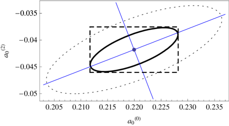
Figure 14: The one and two standard deviation ellipses (thick and dashed lines, respectively) in the $(a_{0}^{(0)},a_{0}^{(2)})$ plane. The square covers the uncertainties of our best results in Eq.(32), obtained from the uncorrelated expressions in Eq.(31).

For the sake of comparison, we list in the sixth column our results from KPY08, where we did not impose the GKPY equations nor did we add the several improvements to the amplitudes and the data implemented in this work. Note that the low energy parameters are quite consistent with our previous results, i.e. many central values lie within one standard deviation of our KPY08 results, and most of them overlap within one standard deviation. There are, of course, the expected exceptions: first, the $\delta_{0}^{(0)}(M_{K}^{2})-\delta_{0}^{(2)}(M_{K}^{2})$ central value changes by 3 standard deviations, mostly due to the fact that we have discarded here the controversial $K\rightarrow\pi\pi$ datum. Next, the S0 slope $b_{0}^{(0)}$ changes by two standard deviations, and this is mostly due to the inclusion of the isospin violation correction in the low energy $K_{\ell 4}$ data. One could have expected that the scattering length $a_{0}^{(0)}$ may have suffered a large shift for the same reason, but it has only decreased about a third of a standard deviation. Hence, most of the change due to the $K_{\ell 4}$ isospin correction is concentrated on the slope parameter. In addition, as we already anticipated, both D wave scattering lengths have decreased by roughly 2 standard deviations.

Although it will be commented in detail in the discussion section, let us note that these new results are in much better agreement with the results in Bern , than were those in KPY08.

As commented in Sec. V, we can also check here that the new uncertainties are slightly smaller, but only by 10-15%, than in KPY08, due to: discarding the $K\rightarrow\pi\pi$ conflicting input, keeping the S0 Adler zero fixed, and the more precise NA48/2 published data. The $a_{0}^{(0)}-a_{0}^{(2)}$ uncertainty in (32) has decreased by almost 50%, although this is not only due to our improvement of the S0 wave, but mainly to the fact that we are now calculating it differently, using Eqs. (31).

VI.2 Determination of Adler zeros

As already explained, chiral symmetry requires the existence of zeros in the amplitude close to $s=0$ for the scalar waves S0 and S2 Adler:1964um . We have explicitly factorized them in our amplitudes at $s_{A}^{S0}=z_{0}^{2}/2$ and $s_{A}^{S2}=2z_{2}^{2}$, see Eqs. (6) or (33) and (37). As a starting point, we have first fixed them to the ChPT leading order estimate by setting $z_{0}=z_{2}=M_{\pi}$ for the UFD parametrizations. We then used these parametrizations inside Roy or GKPY equations to recalculate the position of these Adler zeros, which were listed in the first two columns of Table 2.

In previous works, we allowed the $z_{0}$ and $z_{2}$ parameters to change in the CFD set, expecting them to be accurately fixed by imposing the dispersion relations. Unfortunately, as discussed in Sect. V.2, this does not work for the S0 wave. The reason is that its Adler zero is very close to the left cut, in a region where, on the one hand, neither Roy nor GKPY equations provide a precise determination of the zero position (see Table 2) and, on the other hand, the conformal expansion converges badly. For that reason, we have simply kept the S0 parameter $z_{0}$ fixed to $M_{\pi}$ both on the UFD and CFD sets. Being so far from the threshold region, this effect is irrelevant inside the dispersive integrals. Thus, only the S2 Adler zero is allowed to change when obtaining the CFD set, but only within the UFD uncertainties obtained from Roy and GKPY equations.

In this section we go one step further and we finally provide, in the last two columns of Table 2, the value of the S0 and S2 wave Adler zeros obtained when the CFD set is used inside Roy and GKPY equations. The CFD S0 zero is closer to its expected position (around 80 MeV) than the UFD result, but note that the uncertainty gets worse because of this displacement towards the left cut. In summary, we do not have enough precision to pin down the location of this S0 Adler zero accurately.

In contrast, the S2 Adler zero is determined quite precisely by GKPY equations (and to a lesser extent by Roy equations), and the resulting $z_{2}$ parameter, if allowed to vary, is almost identical to its UFD determination. Thus, as explained in Section V.2, we have allowed $z_{2}\sqrt{2}$ to vary within the weighted average between the GKPY and Roy equation results of the UFD set. The resulting Adler zero, when read directly from the CFD parametrization is $\sqrt{s_{A}^{S2}}=z_{2}\sqrt{2}=201\pm 5\,{\mbox{MeV}\,}$, which is almost identical to the values obtained by using the CFD set inside Roy or GKPY equations—listed in Table 2. This confirms that it is correct to identify the Adler zero with the $z_{2}\sqrt{2}$ term in our S2 wave conformal parametrization.

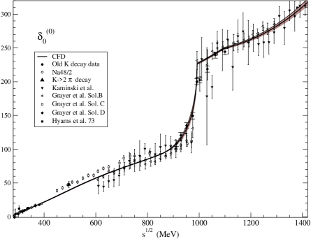
Figure 15: The new constrained fit (CFD) for the S0 wave versus the existing phase shift data from pipidata ; pipidata2 . The dark band covers the uncertainties,

VII Discussion

First of all, we want to remark that ours is just a data analysis, and we are not predicting the value of any observable, just determining them from experiment. In contrast to other approaches Bern , we are not solving FDR, Roy or GKPY equations, but just imposing them as constraints on the data analysis. Actually, all these equations have been obtained with several approximations, for instance, they are obtained in the isospin limit, and we only expect them to describe the real world up to some uncertainty of the order of 3%. In addition, all Roy equations studies we are aware of—including this one—neglect any inelasticity to four or more pion states below the two kaon threshold. This is certainly a very small effect, but is nevertheless an approximation.

Being a data analysis, our parametrizations change when the data changes. In particular, in this work we have updated the NA48/2 data Batley:2007zz with their final results ULTIMONA48 , which have smaller uncertainties. In addition, we have incorporated the threshold-enhanced isospin correction in Colangelo:2008sm to all $K_{\ell 4}$ data. Moreover, we have discarded the controversial $K\rightarrow\pi\pi$ datum Aloisio:2002bs . Furthermore, the increased precision provided by the once-subtracted dispersion relations that we have introduced in this work, requires an improved parametrization with a continuous derivative matching. This additional constraint and the requirement that the output of the dispersion relations should satisfy the elastic unitarity bound—which is automatic in the input parametrizations—, has made us also add an additional parameter to the S0 wave parametrization at low energies. As we will see below, the S0 wave parametrization at intermediate energies favors the “dip-scenario” for the S0 inelasticity between 1000 and 1100 MeV. In this discussion section we will show in detail the new CFD set, particularly the S0 wave, comparing it to other works, and we will discuss the consequences of these modifications.

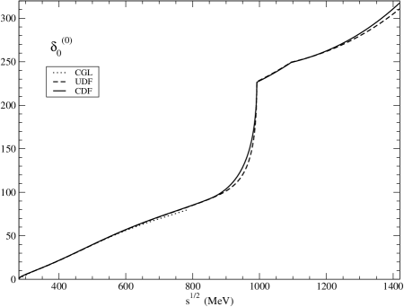
Figure 16: Comparison between the phase of the constrained (CFD) and unconstrained (UFD) Fit to Data for the S0 wave. We also plot the phase from the Roy equations analysis in Bern .

VII.1 The new CFD S0 wave

In Fig. 15 we show the resulting CFD S0 wave from threshold up to 1420 MeV, versus the data from different sets in the literature pipidata ; pipidata2 . Note the smooth matching at 850 MeV and the kink at $K\bar{K}$ threshold. This is in contrast with our old KPY08 results, already shown in Fig. 3, which have a spurious kink at the matching point (932 MeV in that work), and a much less pronounced kink at $K\bar{K}$ threshold. The difference between the UFD and CFD S0 wave phase shift at low energies, which we showed in Fig. 2, is almost imperceptible.

To ease the comparison of this CFD results with the UFD set for all energies, we have plotted their central values together in Fig. 16. It can be noted that the change above $K\bar{K}$ threshold is again almost imperceptible up to 1200 MeV. The only sizable differences between the phase of the UFD and CFD parametrizations are above 1200 MeV, where our parametrizations are less reliable since Roy and GKPY Eqs. only extend up to 1115  MeV, and on the sharp phase rise in the 900 MeV to $2m_{K}=992\,$MeV region due to the $f_{0}(980)$ resonance, which is clearly less steep in the CFD case than in the UFD. The latter is one of the reasons why the CFD solution satisfies GKPY equations well within uncertainties, but the UFD lies somewhere around 2 standard deviations away (see Tables 1 and 3, respectively).

In addition, we are also showing in Fig. 16 the results from Bern , which are in good agreement with ours, but lie slightly lower only above 550 MeV (see discussion below). Actually, our CFD solution does not show the “hunchback“ between 500 and 900 MeV seen in KPY08, as already shown in Fig. 3.

Concerning the S0 inelasticity, we show in Fig. 17 the difference between the UFD and CFD sets. It can be noticed that the difference lies essentially within the uncertainties (gray area), although the “dip” structure above 1000 MeV becomes even deeper in the CFD set. Finally, in Fig. 18 we show the CFD inelasticity versus all the existing experimental data.

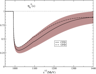
Figure 17: Comparison between the UFD and CFD S0 wave inelasticity. The gray area corresponds to the CFD uncertainty. A similar size area should be associated to the UFD result, but for clarity we only show its central value. Note the dip structure between 1 and 1.1 GeV.

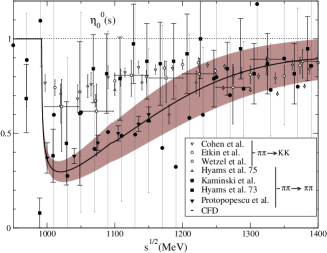
Figure 18: CFD S0 wave inelasticity versus experimental data.

Since the UFD set was already providing a good description of the inelasticity data obtained from $\pi\pi\rightarrow\pi\pi$ experiments, as shown in Fig. 4, so it does the CFD. For the same reason, it also fails to reproduce the inelasticity data from $\pi\pi\rightarrow K\bar{K}$, as we had already shown for the UFD case in Fig. 5. Note that this is due to the fact that both our UFD and CFD solutions show a “dip” structure between 1 and 1.1 GeV, which is seen in the data coming from $\pi\pi\rightarrow\pi\pi$, but not in those coming from $\pi\pi\rightarrow K\bar{K}$. This is a longstanding problem (see Au:1986vs and references therein) that we will address in the next subsection, showing that the “non-dip” scenario is not able to satisfy the dispersive representation well even when allowing for a large deviation from the phase shift data.

VII.2 S0 inelasticity: the “non-dip” scenario is disfavored

In order to show how much the “non-dip” scenario is disfavored, we will first repeat the same procedure of this whole paper, but starting from the S0 inelasticity fitted to the “non-dip” data, as shown in Fig. 19, while keeping the same UFD parametrization for all other waves and for the S0 phase. We will refer to this set as “ndUFD”. The resulting averaged discrepancies $\bar{d}^{2}_{i}$ are relatively similar to those in Table 1 for our UFD, except for the S0 wave GKPY equations up to $\sqrt{s}\leq 1100\,$MeV, whose averaged $\bar{d}^{2}_{i}$ rises from 2.42 to 4.77. This already disfavors the “non-dip” scenario.

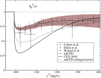
Figure 19: S0 wave inelasticity versus the “non-dip” $\pi\pi\rightarrow K\bar{K}$ data. We first show the “ndUFD” set obtained from a fit to these “non-dip” data. Next, we show the “ndCFD” set obtained with enlarged errors to try to fulfill dispersion relations. This constrained fit satisfies the dispersive constraints better but does not describe these “non-dip” data, coming closer to the best CFD set, which actually describes the alternative “dip” data from $\pi\pi\rightarrow\pi\pi$.

Of course, the “dip scenario” UFD set was not doing very well either, but we were able to improve it by constraining the fit to data with dispersion relations, i.e., the CFD set. One could wonder if a similar quality fit can also be obtained by imposing the dispersive constraints, but starting from the “ndUFD”. Thus, we followed again the procedure described in previous sections, but to arrive now to a “ndCFD” set. Surprisingly, the S0 inelasticity barely changes, but the improvement comes from a bigger variation of the phase in the two-kaon subthreshold region. The resulting average discrepancies $\bar{d}^{2}_{i}$ come in general larger than for our CFD set, sometimes by a factor of two, but still below 1. This may look like an agreement, but one should not be misguided now by these relatively low averaged $\bar{d}^{2}_{i}$ because, contrary to the CFD set where discrepancies are below 1 uniformly over the whole energy region, for the ndCFD set they are larger in the $f_{0}(980)$ resonance region.

In particular, in the interval between 950 and 1050 MeV, for the CFD set, the GKPY S0 equation have $\bar{d}^{2}=1.02$, whereas the ndCFD set has $\bar{d}^{2}=3.49$. This averaged discrepancy is unacceptable now, since this time we are using the dispersion relations as constraints of our fits. In addition, the crossing sum rule in Eq. (16) grows to $\bar{d}_{I}^{2}=2.0$.

Furthermore, as we show in Fig. 20, in the region from 900 MeV up to $K\bar{K}$ threshold, the resulting phase of this ndCFD scenario lies above all data points with a $\chi^{2}/{\rm\#points}=3.4$, which is a very bad fit. In contrast, the CFD set has $\chi^{2}/{\rm\#points}=0.98$ in this region and is just a small modification from the UFD phase, which has $\chi^{2}/{\rm\#points}=0.63$. Moreover, the ndCFD parameters lie far from the original ndUFD ones, with the $c$ parameter more than 6 standard deviations away from its ndUFD value. These numbers clearly show the incompatibility of the ndCFD set with the S0 wave $\pi\pi\rightarrow\pi\pi$ phase-shift scattering data. This disagreement cannot be mended by adding systematic uncertainties, since in this region we had already included large systematic uncertainties (see KPY08 and PY05 for details) and all points have total uncertainties of more than 10 degrees.

Figure 20: Comparison of the UFD, CFD and ndCFD solutions for the S0 phase in the 850 to 1050 MeV region. Note that the ndCFD parametrization is largely inconsistent with data, despite the fact we are plotting the PY05 averaged data, that includes our estimations of the large dominant systematic uncertainties.

One could wonder if our minimization procedure, that was good enough to reach $\bar{d}_{i}^{2}<1$ for the dip scenario, is badly tuned for the “non-dip” one. This, of course is the role of the $W_{i}$ weights in Eq. (21). For this reason we have repeated the above procedure adding additional weight to the GKPY S0 wave equation above 900 MeV. The resulting “ndCFD2” yields $\bar{d}^{2}=2.06$ for the GKPY S0 equation. Besides, the crossing sum rule in Eq.  (16) is also $\bar{d}_{i}^{2}=1.43$. Although they still disfavor this solution, these numbers by themselves are not too bad. However, the phase shift data between 950 and 1050 MeV has $\chi^{2}/{\rm\#points}=5.9$, so that it is described even worse than with the previous ndCFD.

Since we cannot fix the dispersive constraints without spoiling the data phase description, we have allowed, as a final check, for larger errors in the inelasticity parameters of the “non-dip” scenario, and applied the dispersive constraints. In so doing, we can obtain $\bar{d}_{i}^{2}<1$ uniformly over all energy regions for all GKPY equations except for the S0 wave between 950 to 1050 MeV, for which we obtain $1.42$. However, the central value of the inelasticity for the resulting constrained “non-dip” fit starts developing a dip as seen in Fig. 19. Therefore, we describe neither the “non-dip” nor the “dip” scenario.

In conclusion, the non-dip scenario, even when constrained with dispersion relations, is not able to describe the data and simultaneously satisfy Forward Dispersion Relations, Roy and GKPY equations, plus certain crossing sum rules.

VII.3 Comparison with other works.

The results listed in Table LABEL:tab:thresholdparameters for threshold parameters are remarkably compatible with the predictions of Bern using Chiral Perturbation Theory and Roy equations:

$$a_{0}^{(0)}=0.220\pm 0.005,\qquad a_{0}^{(2)}=-0.0444\pm 0.0010.$$

The agreement with that reference has also improved a great deal since the $\delta_{0}^{(0)}(M_{K}^{2})-\delta_{0}^{(2)}(M_{K}^{2})=(47.3\pm 0.9)^{\circ}$ value, obtained directly from our CFD set, is now completely consistent with their value of $(47.7\pm 1.5)^{\circ}$. Essential for that agreement is, of course, not to consider the $K\rightarrow\pi\pi$ datum. Also, all the D wave threshold parameters are now in good agreement with those used in Bern . The remaining differences with respect to that work are rather small: the largest one is a 2.1 standard deviation disagreement, with respect to their predicted value $b_{1}=(5.67\pm 0.13)\times 10^{-3}$. In general, and up to 500 MeV, the results of Bern fall within roughly one standard deviation of our analysis. For instance, at the kaon mass, our CFD S0 wave phase shift is $\delta_{0}^{(0)}(M_{K})=39.1\pm 0.6^{\circ}$, identical to theirs to the last digit, but our S2 wave is $\delta_{0}^{(2)}(M_{K})=-8.2\pm 0.6^{\circ}$, $0.3$ degrees more than theirs, which is half an standard deviation. This good agreement does not deteriorate much above that energy. For instance, at 800 MeV, which is their matching point between the calculated phase shifts and their input, they use an input value of $\delta_{0}^{(0)}=82.3\pm 3.4^{\circ}$. In contrast, we obtain $\delta_{0}^{(0)}=85.2\pm 0.5^{\circ}$ directly from the CFD set, whereas we find $\delta_{0}^{(0)}=85.7\pm 1.6^{\circ}$ when using the same CFD set inside GKPY equations, that is, one of their standard deviations. Above 800 MeV their amplitudes are part of the input and not solutions of Roy equations.

Finally, we would like to remark that our best values for the scalar scattering lengths in Eq. (32), are in very good agreement with the experimental results from pionic atoms Adeva:2007zz ; Adeva:2005pg , that yield:

$$a_{0}^{(0)}-a_{0}^{(2)}=0.280\pm 0.013{\rm(St.)}\pm 0.008{\rm(Syst.)}\,M_{\pi}^{-1},$$

$$a_{0}^{(0)}-a_{0}^{(2)}=0.264^{+0.033}_{-0.020}\,M_{\pi}^{-1},$$

or $K_{3\pi}$ decays Cabibbo:2005ez :

$$a_{0}^{(0)}-a_{0}^{(2)} = 0.2571\pm 0.0048{\rm(St.)}\qquad$$

$$\qquad\pm 0.0025{\rm(Syst.)}\pm 0.0014{\rm(Ext.)}\,M_{\pi}^{-1}.$$

Had we used them as additional constraints with the statistical and systematic errors added linearly as we did with other decays, the difference with our best results would have been barely modified.

As we commented in Sect. III.2, the phase difference $\delta_{0}^{(0)}(M_{K}^{2})-\delta_{0}^{(2)}(M_{K}^{2})=(52.5\pm 0.8_{\rm exp}\pm 2.8_{\rm exp})^{\circ}$ has been recently re-analyzed Cirigliano:2009rr . This is a considerable shift from the previous value of $(57.27\pm 0.82_{\rm exp.}\pm 3_{\rm rad.}\pm 1_{\rm ChPT\,appr.})^{\circ}$, in much better agreement with ours and other previous dispersive analyses. Note that the new number is also in good agreement with our results in Table LABEL:tab:thresholdparameters.

VIII Summary

In this work, we have presented the derivation of a once-subtracted set of Roy-like dispersion relations—the GKPY equations. We have shown and explained that above 450 MeV, and up to 1115 MeV, they provide stronger constraints on $\pi\pi$ scattering amplitudes than other existing sets of dispersion relations.

We have then applied these new equations as constraints in our fits to data—together with the standard Roy equations and Forward Dispersion relations—in order to obtain a precise description of $\pi\pi$ scattering amplitudes. In contrast to previous works, we have extended the Roy and GKPY equations analysis from 932 MeV up to their applicability limit of 1100 MeV. Forward Dispersion Relations are considered up to 1420 MeV.

We have also made use of the final and very precise data on $K_{\ell 4}$ decays from NA48/2, including the isospin violation corrections proposed in Colangelo:2008sm , and we have removed a conflicting data point from $K\rightarrow 2\pi$ decay. With these changes in the data selection, most of the disagreement with previous Roy equation calculations Bern has disappeared below 800 MeV. The largest discrepancy that remains is on the P wave slope parameter, but just at the two standard deviation level.

In addition, we have improved our S0 wave parametrization to ensure a continuous matching between the low and intermediate energy parametrizations. Both parametrizations have been made more flexible, which allows the phase and inelasticity to include contributions from states different from $\pi\pi$ and $K\bar{K}$, above the $K\bar{K}$ threshold.

There are two sets of fits to data: unconstrained (UFD), or constrained with dispersion relations (CFD). In the UFD set each wave is independent of all others, but dispersion relations are satisfied only up to the two sigma level (in the sense explained in the text). In contrast, the CFD waves are all correlated, but they fulfill all dispersion relations under consideration within less than one standard deviation in the whole energy region. The CFD set can be considered as a very precise parametrization of experimental data consistent with the requirements of analyticity, unitarity and crossing symmetry. Using this CFD set as an input in different sum rules and the dispersion relations themselves, we have also provided a precise determination of phases in the elastic regime, threshold parameters and Adler zeros.

In addition, and concerning the conflicting data for the S0 wave inelasticity between the two-kaon threshold and 1100 MeV, the use of the new GKPY equations has allowed us to show that the sudden drop around 1050 MeV in the S0 wave inelasticity, or “dip solution”, is clearly favored with respect to the “non-dip” solution. Actually, for the “non-dip” inelasticity scenario to fulfill dispersion relations, it would require a very poor description of the phase shift data, even when allowing for large systematic uncertainties.

In conclusion, we provide fits to data in terms of simple and ready to use parametrizations for the S0, S2, P, D0, D2 and F partial waves, between threshold and 1420 MeV. Additional simple Regge parametrizations are given above that energy. In particular, the CFD set satisfies remarkably well all the analyticity and crossing symmetry constraints in the form of once and twice subtracted Roy equations and Forward Dispersion Relations.

Appendix A Partial wave parametrizations

In the following, we provide the parametrizations we use for each partial wave, and then, the parameters for the UFD and CFD sets. For brevity, we do not explain again why a specific parametrization for each wave has been chosen, since such details can be found in KPY08 Kaminski:2006qe . In what follows we use $M_{\pi}=139.57$ MeV, $M_{K}=496$ MeV and $M_{\eta}=547.51$ MeV.

A.1 S0 wave

This wave has been thoroughly discussed in the main text. However, for the sake of completeness, we repeat here the form of the parametrizations and provide the values of the parameters for the UFD and CFD sets in Table 4.

For this wave we have set the matching point between the intermediate and low energy parametrizations at $s_{M}^{1/2}=0.85\,{\mbox{GeV}\,}$. Thus, at low energies $s\leq s_{M}$, we use:

$$\cot\delta_{0}^{(0)}(s)=\frac{s^{1/2}}{2k}\frac{M_{\pi}^{2}}{s-\frac{1}{2}z_{0}^{2}}\times$$ (33)

$$\left\{\frac{z_{0}^{2}}{M_{\pi}\sqrt{s}}+B_{0}+B_{1}w(s)+B_{2}w(s)^{2}+B_{3}w(s)^{3}\right\},$$

$$w(s)=\frac{\sqrt{s}-\sqrt{s_{0}-s}}{\sqrt{s}+\sqrt{s_{0}-s}},\qquad s_{0}=4M_{K}^{2}.$$ (34)

Above that energy, and up to 1.42 GeV, we use the KPY06 polynomial parametrization for the phase shift, but with one more term in the expansion. For definiteness, we provide here the polynomial parametrization once it has been matched to Eq. (33) above, by imposing continuity and a continuous derivative at $s=s_{M}$, namely

$$\delta_{0}^{(0)}(s)=\left\{\begin{array}[]{ll}\displaystyle{d_{0}\left(1-\frac{|k_{2}|}{k_{M}}\right)^{2}+\delta_{M}\,\frac{|k_{2}|}{k_{M}}\left(2-\frac{|k_{2}|}{k_{M}}\right)+|k_{2}|(k_{M}-|k_{2}|)\left(8\delta_{M}^{\prime}+c\frac{(k_{M}-|k_{2}|)}{M_{K}^{3}}\right)},&(0.85\,{\rm GeV})^{2}<s<4M_{K}^{2},\\ \\ \displaystyle{d_{0}+B\frac{k_{2}^{2}}{M_{K}^{2}}+C\frac{k_{2}^{4}}{M_{K}^{4}}}+D\,\theta(s-4M_{\eta}^{2})\frac{k_{3}^{2}}{M_{\eta}^{2}},&4M_{K}^{2}<s<(1.42{\mbox{GeV}\,})^{2},\end{array}\right.$$ (35)

where $k_{2}=\sqrt{s/4-M_{K}^{2}}$. Note that we have defined $\delta_{M}=\delta(s_{M})$ and $\delta_{M}^{\prime}=d\delta(s_{M})/ds$, which are obtained from Eq. (33), and $k_{M}=|k_{2}(s_{M})|$.

Finally, we assume an elastic S0 wave, $\eta_{0}^{(0)}=1$, up to the two-kaon threshold, whereas above that energy, we use:

$$\eta_{0}^{(0)}(s)=\exp\bigg{[}\frac{-k_{2}(s)}{s^{1/2}}\left(\tilde{\epsilon}_{1}+\tilde{\epsilon}_{2}\,\frac{k_{2}}{s^{1/2}}+\tilde{\epsilon}_{3}\,\frac{k_{2}^{2}}{s}\right)^{2}$$ (36)

$$-\tilde{\epsilon}_{4}\theta(s-4M_{\eta}^{2})\frac{k_{3}(s)}{s^{1/2}}\bigg{]}.$$

We have collected the values of the parameters for the UFD and CFD set in Table 4.

S0 wave	UFD	CFD
$B_{0}$	$7.26\pm 0.23$	$7.14\pm 0.23$
$B_{1}$	$-25.3\pm 0.5$	$-25.3\pm 0.5$
$B_{2}$	$-33.1\pm 1.2$	$-33.2\pm 1.2$
$B_{3}$	$-26.6\pm 2.3$	$-26.2\pm 2.3$
$z_{0}$	$M_{\pi}$	$M_{\pi}$
$d_{0}$	$(227.1\pm 1.3)^{\circ}$	$(226.5\pm 1.3)^{\circ}$
$c$	$(-660\pm 290)^{\circ}$	$(-81\pm 294)^{\circ}$
$B$	$(94.0\pm 2.3)^{\circ}$	$(93.3\pm 2.3)^{\circ}$
$C$	$(40.4\pm 2.9)^{\circ}$	$(48.7\pm 2.9)^{\circ}$
$D$	$(-86.9\pm 4.0)^{\circ}$	$(-88.3\pm 4.0)^{\circ}$
$\tilde{\epsilon}_{1}$	$4.7\pm 0.2$	$4.9\pm 0.2$
$\tilde{\epsilon}_{2}$	$-15.0\pm 0.8$	$-15.1\pm 0.8$
$\tilde{\epsilon}_{3}$	$4.7\pm 2.6$	$4.7\pm 2.6$
$\tilde{\epsilon}_{4}$	$0.38\pm 0.34$	$0.32\pm 0.34$

Table 4: S0 wave parameters for the UFD and CFD sets. The first four lines correspond to the low energy parametrization, $\sqrt{s}\leq 0.85\,{\mbox{GeV}\,}$, and the last nine to the parametrization up to $\sqrt{s}=1.42\,{\mbox{GeV}\,}$.

A.2 S2 wave

As we have already done with the S0 wave, we have also set the matching point between intermediate and low energy parametrizations for this wave at $s_{M}^{1/2}=850\,{\mbox{MeV}\,}$. Thus, at energies $s^{1/2}\leq s_{M}^{1/2}$ we use:

$$\cot\delta^{(2)}_{0}(s)=\frac{s^{1/2}}{2k}\frac{M_{\pi}^{2}}{s-2z_{2}^{2}}\left\{B_{0}+B_{1}w_{l}(s)\right\},$$

$$w_{l}(s)=\frac{\sqrt{s}-\sqrt{s_{l}-s}}{\sqrt{s}+\sqrt{s_{l}-s}},\quad s_{l}^{1/2}=1.05\,{\mbox{GeV}\,},$$ (37)

whereas at intermediate energies, $850\,{\mbox{MeV}\,}\leq s^{1/2}\leq 1420\,{\mbox{MeV}\,}$, we use:

$$\cot\delta^{(2)}_{0}(s)=\frac{s^{1/2}}{2k}\frac{M_{\pi}^{2}}{s-2z_{2}^{2}}\times$$

$$\left\{B_{h0}+B_{h1}[w_{h}(s)-w_{h}(s_{M})]+B_{h2}[w_{h}(s)-w_{h}(s_{M})]^{2}\right\},$$

where

$$w_{h}(s)=\frac{\sqrt{s}-\sqrt{s_{h}-s}}{\sqrt{s}+\sqrt{s_{h}-s}},\quad s_{h}^{1/2}=1.42\,{\mbox{GeV}\,},$$

$$B_{h0}=B_{0}+B_{1}w_{l}(s_{M}),\quad B_{h1}=B_{1}\left.\frac{\partial w_{l}(s)}{\partial w_{h}(s)}\right|_{s=s_{M}}$$

$$B_{h1}=B_{1}\frac{s_{l}}{s_{h}}\frac{\sqrt{s_{h}-s_{M}}}{\sqrt{s_{l}-s_{M}}}\left(\frac{\sqrt{s_{M}}+\sqrt{s_{h}-s_{M}}}{\sqrt{s_{M}}+\sqrt{s_{l}-s_{M}}}\right)^{2}$$ (38)

Note that, with these definitions, both the parametrization and its derivative are continuous at the matching point.

Note that we have explicitly factorized the Adler zero at $s_{A}=2z_{2}^{2}$. For the unconstrained fit, $z_{2}$ is fixed to the pion mass. As explained in the main text in Sect. V.2, we then calculate the Adler zero position using Roy and GKPY equations, and feed the weighted average into the constrained fit. This change is very small in terms of the total values and uncertainties of other quantities, but it is relevant in the differences when calculating the fulfillment of GKPY equations.

For the inelasticity, we set $\eta_{0}^{(2)}(s)=1$ for $s$ below $\hat{s}=(1.05\,{\mbox{GeV}\,})^{2}$ and above that energy we use the empirical fit:

$$\eta_{0}^{(2)}(s)=1-\epsilon(1-\hat{s}/s)^{3/2}.$$

The S2 wave parameters for UFD and CFD sets are given in Table 5.

S2 wave	UFD	CFD
$B_{0}$	$-80.4\pm 2.8$	$-79.4\pm 2.8$
$B_{1}$	$-73.6\pm 10.5$	$-63.0\pm 10.5$
$z_{2}$	$M_{\pi}$	$143.5\pm 3.2\,{\mbox{MeV}\,}$
$B_{h2}$	$112\pm 38$	$32\pm 38$
$\epsilon$	$0.28\pm 0.12$	$0.28\pm 0.12$

Table 5: S2 wave parameters for the UFD and CFD sets.

A.3 P wave

For this wave we have set the matching point between low and intermediate energy parametrizations at $s_{M}^{1/2}=2M_{K}$. Thus, at low energies $s^{1/2}\leq 2M_{K}$, we use:

$$\cot\delta_{1}(s)=\frac{s^{1/2}}{2k^{3}}(M_{\rho}^{2}-s)\left\{\frac{2M_{\pi}^{3}}{M_{\rho}^{2}\sqrt{s}}+B_{0}+B_{1}w(s)\right\},$$

$$w(s)=\frac{\sqrt{s}-\sqrt{s_{0}-s}}{\sqrt{s}+\sqrt{s_{0}-s}},\quad s_{0}^{1/2}=1.05\,{\mbox{GeV}\,},$$ (39)

where the $\rho$ mass is fixed to $M_{\rho}=773.6\pm 0.9\,{\mbox{MeV}\,}$. At intermediate energies, $2M_{K}\leq s^{1/2}\leq 1420\,{\mbox{MeV}\,}$, we use a purely phenomenological parametrization:

$$\delta_{1}(s)=\lambda_{0}+\lambda_{1}\left(\sqrt{s}/2M_{K}-1\right)+\lambda_{2}\left(\sqrt{s}/2M_{K}-1\right)^{2},$$

$$\eta_{1}(s)=1-\epsilon_{1}\sqrt{1-4M_{K}^{2}/s}-\epsilon_{2}(1-4M_{K}^{2}/s),$$ (40)

where $\lambda_{0}$ is fixed from the value of $\delta_{1}(4M_{K}^{2})$ obtained from the low energy parametrization, so that the phase shift is continuous. Note the possible presence of a discontinuity in the derivative, allowed by the presence of the $K\bar{K}$ threshold. The values of the UFD and CFD parameters are given in Table 6.

P wave	UFD	CFD
$B_{0}$	$1.055\pm 0.011$	$1.043\pm 0.011$
$B_{1}$	$0.15\pm 0.05$	$0.19\pm 0.05$
$\lambda_{1}$	$1.57\pm 0.18$	$1.39\pm 0.18$
$\lambda_{2}$	$-1.96\pm 0.49$	$-1.70\pm 0.49$
$\epsilon_{1}$	$0.10\pm 0.06$	$0.00\pm 0.06$
$\epsilon_{2}$	$0.11\pm 0.11$	$0.07\pm 0.11$

Table 6: P wave parameters for the UFD and CFD sets.

A.4 The D0 wave

As it was the case for the P wave, the matching energy between low and intermediate energies is now taken at $s_{M}^{1/2}=2M_{K}$. At low energies, $s^{1/2}\leq 2M_{K}$, we parametrize this wave by:

$$\cot\delta_{2}^{(0)}(s)=\frac{s^{1/2}}{2k^{5}}(M_{f_{2}}^{2}-s)M_{\pi}^{2}\left\{B_{0}+B_{1}w(s)\right\},$$

$$w(s)=\frac{\sqrt{s}-\sqrt{s_{0}-s}}{\sqrt{s}+\sqrt{s_{0}-s}},\quad s_{0}^{1/2}=1.05\,{\mbox{GeV}\,},$$ (41)

where the mass of the $f_{2}(1270)$ resonance is fixed at $M_{f_{2}}=1275.4\,{\mbox{MeV}\,}$. In the intermediate region, $2M_{K}\leq s^{1/2}\leq 1420\,{\mbox{MeV}\,}$, we use a rather similar parametrization:

$$\cot\delta_{2}^{(0)}(s)=\frac{s^{1/2}}{2k^{5}}(M_{f_{2}}^{2}-s)M_{\pi}^{2}\left\{B_{0h}+B_{1h}w_{h}(s)\right\},$$

$$w_{h}(s)=\frac{\sqrt{s}-\sqrt{s_{h}-s}}{\sqrt{s}+\sqrt{s_{h}-s}},\quad s_{h}^{1/2}=1.45\,{\mbox{GeV}\,}.$$ (42)

Imposing continuity at the matching point fixes $B_{h0}$ from the value of $\delta_{2}^{(0)}(4M_{K}^{2})$ obtained from the low energy parametrization. We take the inelasticity to be different from 1 only for $s>4M_{K}^{2}$, in which case we write:

$$\eta_{2}^{(0)}=1-\epsilon\left(\frac{1-4M_{K}^{2}/s}{1-4M_{K}^{2}/M_{f_{2}}^{2}}\right)^{5/2}\left[1+r\left(1-\frac{k_{2}(s)}{k_{2}(M_{f_{2}}^{2})}\right)\right].$$ (43)

The parameters of the D0 wave are given in Table 7.

D0 wave	UFD	CFD
$B_{0}$	$12.47\pm 0.12$	$12.40\pm 0.12$
$B_{1}$	$10.12\pm 0.16$	$10.06\pm 0.16$
$B_{h1}$	$43.7\pm 1.8$	$43.2\pm 1.8$
$\epsilon$	$0.284\pm 0.030$	$0.254\pm 0.030$
$r$	$2.54\pm 0.31$	$2.29\pm 0.31$

Table 7: D0 wave parameters for the UFD and CFD sets.

A.5 The D2 wave

We use the following parametrization from threshold up to $1420\,{\mbox{MeV}\,}$:

$$\cot\delta_{2}^{(2)}(s)=\frac{s^{1/2}}{2k^{5}}\times\hskip 113.81102pt$$

$$\qquad\times\frac{M_{\pi}^{4}\,s}{4(M_{\pi}^{2}+\Delta^{2})-s}\left\{B_{0}+B_{1}w(s)+B_{2}w(s)^{2}\right\},$$

$$w(s)=\frac{\sqrt{s}-\sqrt{s_{0}-s}}{\sqrt{s}+\sqrt{s_{0}-s}},\quad s_{0}^{1/2}=1.45\,{\mbox{GeV}\,},$$ (44)

and we consider that the inelasticity differs from 1 for $s^{1/2}>1.05\,{\mbox{GeV}\,}$, as follows:

$$\eta_{2}^{(2)}(s)=1-\epsilon(1-\hat{s}/s)^{3},\quad\hat{s}^{1/2}=1.05\,{\mbox{GeV}\,},$$ (45)

which is almost negligible up to 1.25 GeV . The values of the parameters for the UFD and CFD sets are given in Table 8.

D2 wave	UFD	CFD
$B_{0}$	$(2.4\pm 0.5)\,10^{3}$	$(4.1\pm 0.5)\,10^{3}$
$B_{1}$	$(7.8\pm 1.0)\,10^{3}$	$(8.6\pm 1.0)\,10^{3}$
$B_{2}$	$(23.7\pm 4.2)\,10^{3}$	$(25.5\pm 4.2)\,10^{3}$
$\Delta$	$196\pm 25\,{\mbox{MeV}\,}$	$233\pm 25\,{\mbox{MeV}\,}$
$\epsilon$	$0.2\pm 0.2$	$0.0\pm 0.2$

Table 8: D2 wave parameters for the UFD and CFD sets.

A.6 The F wave

We neglect the inelasticity up to $1420\,{\mbox{MeV}\,}$ and simply use the following parametrization from threshold:

$$\cot\delta_{3}(s)=\frac{s^{1/2}}{2k^{7}}M_{\pi}^{6}\left\{\frac{2\lambda M_{\pi}}{\sqrt{s}}+B_{0}+B_{1}w(s)\right\},$$

$$w(s)=\frac{\sqrt{s}-\sqrt{s_{0}-s}}{\sqrt{s}+\sqrt{s_{0}-s}},\quad s_{0}^{1/2}=1.45\,{\mbox{GeV}\,}.$$ (46)

The parameters for the UFD and CFD sets are given in Table 9. Note that they do not change at all from one set to another.

F wave	UFD	CFD
$B_{0}$	$(1.09\pm 0.03)\,10^{5}$	$(1.09\pm 0.03)\,10^{5}$
$B_{1}$	$(1.41\pm 0.04)\,10^{5}$	$(1.41\pm 0.04)\,10^{5}$
$\lambda$	$0.051\times 10^{5}$	$0.051\times 10^{5}$

Table 9: F wave parameters for the UFD and CFD sets.

A.7 The G waves

The contribution of the G0 and G2 waves was shown to be completely negligible for the calculations. The details can be found in the Appendix of KPY08 Kaminski:2006qe .

A.8 Regge Parametrizations

Next we show the Regge parametrizations that we use in the high energy region, i.e. above $1420\,{\mbox{MeV}\,}$. The forward $(t=0)$ Regge parametrizations were obtained from fits to high energy data Pelaez:2003ky . For the $t\neq 0$ behavior we Kaminski:2006qe simply covered the uncertainties between the different fits in Rarita:1968zz . These Regge fits are expected to represent experimental data when $1.42\,{\mbox{GeV}\,}\leq s^{1/2}\leq\,20\,{\mbox{GeV}\,}$ and $4M_{\pi}^{2}\geq t\geq-0.4\,{\mbox{GeV}\,}^{2}$, somewhat less reliably for the most negative $t$ values. This is enough to describe the region of interest, that reaches $t=-0.42\,{\mbox{GeV}\,}^{2}$. In particular, for the $\rho$ Regge trajectory, we use the following expression for the imaginary part, which is all we need in the dispersive integrals:

$${\rm Im}\,F^{(I_{t}=1)}(s,t)=\beta_{\rho}\frac{1+\alpha_{\rho}(t)}{1+\alpha_{\rho}(0)}\varphi(t){\rm e}^{bt}\left(\frac{s}{\hat{s}}\right)^{\alpha_{\rho}(t)},$$

$$\alpha_{\rho}(t)=\alpha_{\rho}(0)+t\,\alpha_{\rho}^{\prime}+\frac{1}{2}t^{2}\,\alpha_{\rho}^{\prime\prime},$$

$$\varphi(t)=1+d_{\rho}t+e_{\rho}t^{2},$$ (47)

where we fix:

$$\hat{s}=1\,{\mbox{GeV}\,}^{2},\quad b=2.4\pm 0.2\,{\mbox{GeV}\,}^{-2},$$ (48)

$$\alpha^{\prime}_{\rho}=0.90\,{\mbox{GeV}\,}^{-2},\alpha^{\prime\prime}_{\rho}=-0.3\,{\mbox{GeV}\,}^{-4},$$

$$d_{\rho}=2.4\pm 0.5\,{\mbox{GeV}\,}^{-2},$$

whereas the rest of the parameters are allowed to vary in the fits.

Regge param.	UFD	CFD
$\beta_{\rho}$	$1.22\pm 0.14$	$1.48\pm 0.14$
$\alpha_{\rho}(0)$	$0.46\pm 0.02$	$0.53\pm 0.02$
$\beta_{P}$	$2.54\pm 0.04$	$2.50\pm 0.04$
$c_{P}$	$0.0\pm 1.0\,{\mbox{GeV}\,}^{-2}$	$0.6\pm 1.0\,{\mbox{GeV}\,}^{-2}$
$c_{P^{\prime}}$	$-0.4\pm 0.4\,{\mbox{GeV}\,}^{-2}$	$-0.38\pm 0.4\,{\mbox{GeV}\,}^{-2}$
$\beta_{P^{\prime}}$	$0.83\pm 0.05$	$0.80\pm 0.05$
$\alpha_{P^{\prime}}(0)$	$0.54\pm 0.02$	$0.53\pm 0.02$
$\beta_{2}$	$0.2\pm 0.2$	$0.08\pm 0.2$
$e_{\rho}$	$0\pm 2.5\,{\mbox{GeV}\,}^{-4}$	$2.7\pm 2.5\,{\mbox{GeV}\,}^{-4}$

Table 10: UFD and CFD parameters for the $\rho$, Pomeron and $I=2$ Regge contributions to $\pi\pi$ scattering amplitudes.

For both the Pomeron $P$ and the $P^{\prime}$ pole, we have used for $s^{1/2}=1420\,{\mbox{MeV}\,}$:

$${\rm Im}\,F^{(I_{t}=0)}(s,t)=P(s,t)+P^{\prime}(s,t),$$

$$P(s,t)=\beta_{P}\Psi_{P}(t)\alpha_{P}(t)\frac{1+\alpha_{P}(t)}{2}{\rm e}^{bt}\left(\frac{s}{\hat{s}}\right)^{\alpha_{P}(t)},$$

$$\alpha_{P}(t)=1+t\alpha^{\prime}_{P},\qquad\qquad\Psi_{P}(t)=1+c_{P}t,$$

$$P^{\prime}(s,t)=\beta_{P^{\prime}}\Psi_{P^{\prime}}(t)\frac{\alpha_{P^{\prime}}(t)[1+\alpha_{P^{\prime}}(t)]}{\alpha_{P^{\prime}}(0)[1+\alpha_{P^{\prime}}(0)]}{\rm e}^{bt}\left(\frac{s}{\hat{s}}\right)^{\alpha_{P^{\prime}}(t)},$$

$$\alpha_{P^{\prime}}(t)=\alpha_{P^{\prime}}(0)+t\alpha^{\prime}_{P^{\prime}},\quad\Psi_{P^{\prime}}(t)=1+c_{P^{\prime}}t,$$

where, once again, we fix:

$$\hat{s}=1\,{\mbox{GeV}\,}^{2},\quad b=2.4\pm 0.2\,{\mbox{GeV}\,}^{-2},$$ (50)

$$\alpha^{\prime}_{P}=0.20\pm 0.10\,{\mbox{GeV}\,}^{-2},\alpha^{\prime}_{P^{\prime}}=0.90\,{\mbox{GeV}\,}^{-2},$$

$$c_{P}=0.0\pm 1.0\,{\mbox{GeV}\,}^{-2},c_{P^{\prime}}=-0.4\pm 0.4\,{\mbox{GeV}\,}^{-2},$$

and allow the rest of the parameters to vary in the fits.

Finally, the Regge exchange of isospin two is parametrized as:

$${\rm Im}\,F^{(I_{t}=2)}=\beta_{2}\,{\rm e}^{bt}\left(\frac{s}{\hat{s}}\right)^{\alpha_{\rho}(t)+\alpha_{\rho}(0)-1}.$$ (51)

In Table 10 we show the values of the Regge parameters obtained from the direct fit to high energy data (UFD) and how they are modified when imposing the dispersive constraints in the fits (CFD).

Appendix B Derivation of the once subtracted dispersion relations

A once subtracted dispersion relation for a scattering amplitude of definite isospin $I$ has the following expression:

$$F^{(I)}(s,t)=F^{(I)}(s_{0},t)+\frac{s-s_{0}}{\pi}\int_{4M_{\pi}^{2}}^{\infty}ds^{\prime}\frac{\mbox{Im }F^{(I)}(s^{\prime},t)}{(s^{\prime}-s_{0})(s^{\prime}-s)}\\ +\frac{s-s_{0}}{\pi}\int_{-t}^{-\infty}ds^{\prime}\frac{\mbox{Im }F^{(I)}(s^{\prime},t)}{(s^{\prime}-s_{0})(s^{\prime}-s)},$$ (52)

with $s_{0}$ the subtraction point. This expression assumes that the point $s$ is regular. However, we are especially interested in what happens for $s$ in the physical region, that is, on the cuts of the function $F(s,t)$. The usual prescription is to define the amplitude for physical values of $s$ as:

$$F_{phys}(s,t)=\lim_{\epsilon\rightarrow 0^{+}}F(s+i\epsilon,t).$$

With this prescription, we have:

$$F_{phys}^{(I)}(s,t)=\lim_{\epsilon\rightarrow 0^{+}}F^{(I)}(s+i\epsilon,t)=\\ F^{(I)}(s_{0},t)+\frac{s-s_{0}+i\epsilon}{\pi}\int_{4M_{\pi}^{2}}^{\infty}ds^{\prime}\frac{\mbox{Im }F^{(I)}(s^{\prime},t)}{(s^{\prime}-s_{0})(s^{\prime}-s-i\epsilon)}\\ +\frac{s-s_{0}+i\epsilon}{\pi}\int_{-t}^{-\infty}ds^{\prime}\frac{\mbox{Im }F^{(I)}(s^{\prime},t)}{(s^{\prime}-s_{0})(s^{\prime}-s-i\epsilon)}.$$ (53)

To obtain the physical amplitude, we must take the limit $\epsilon\rightarrow 0^{+}$ in this expression. Suppose $s$ is on the right hand cut (RHC), $4M_{\pi}^{2}<s<\infty$. Since

$$\frac{1}{x\pm i\epsilon}=\hbox{P.P.}\left[\frac{1}{x}\right]\mp i\pi\delta(x),\qquad\epsilon\rightarrow 0^{+},$$

we can write the RHC integral as:

$$\frac{s-s_{0}}{\pi}\,\hbox{P.P.}\int_{4M_{\pi}^{2}}^{\infty}ds^{\prime}\frac{\mbox{Im }F^{(I)}(s^{\prime},t)}{(s^{\prime}-s_{0})(s^{\prime}-s)}+i\,\mbox{Im }F^{(I)}(s,t),$$

whereas the left hand cut (LHC) integral presents no problems when $\epsilon$ vanishes. Then we have

$$F^{(I)}_{phys}(s,t)=F^{(I)}(s_{0},t)+i\,\mbox{Im }F^{(I)}(s,t)\\ +\frac{s-s_{0}}{\pi}\,\hbox{P.P.}\int_{4M_{\pi}^{2}}^{\infty}ds^{\prime}\frac{\mbox{Im }F^{(I)}(s^{\prime},t)}{(s^{\prime}-s_{0})(s^{\prime}-s)}\\ +\frac{s-s_{0}}{\pi}\int_{-t}^{-\infty}ds^{\prime}\frac{\mbox{Im }F^{(I)}(s^{\prime},t)}{(s^{\prime}-s_{0})(s^{\prime}-s)},$$ (54)

thus the dispersive integrals only reconstruct the real part of the amplitude, instead of the total amplitude. Had we chosen $s$ to be on the LHC, the reasoning would be analogous, but the principal value should be taken on the LHC integral, instead of on the RHC one. We finally obtain:

$$\mbox{Re }F_{phys}^{(I)}(s,t)=\mbox{Re }F^{(I)}(s_{0},t)\\ +\frac{s-s_{0}}{\pi}\,\hbox{P.P.}\int_{4M_{\pi}^{2}}^{\infty}ds^{\prime}\frac{\mbox{Im }F^{(I)}(s^{\prime},t)}{(s^{\prime}-s_{0})(s^{\prime}-s)}\\ +\frac{s-s_{0}}{\pi}\,\hbox{P.P.}\int_{-t}^{-\infty}ds^{\prime}\frac{\mbox{Im }F^{(I)}(s^{\prime},t)}{(s^{\prime}-s_{0})(s^{\prime}-s)},$$ (55)

with the principal value taken on the cut on which $s$ lies. This is valid for any $s$ on the cuts of $F^{(I)}(s,t)$, i. e., for physical $s$. We can now recast the LHC integral on the $s$-channel in Eq. (52) in terms of the $u$-channel RHC by renaming the dummy variable $s^{\prime}$ as $u^{\prime}$ in the LHC integral and performing the substitution

$$u^{\prime}\rightarrow 4M_{\pi}^{2}-s^{\prime}-t.$$

Taking both integrands under the same integral sign, and choosing $s_{0}=0$—in analogy with Roy’s derivation—we obtain:

$$\mbox{Re }F^{(I)}(s,t)=\mbox{Re }F^{(I)}(0,t)\\ +\frac{s}{\pi}\int_{4M_{\pi}^{2}}^{\infty}ds^{\prime}\left[\frac{\mbox{Im }F^{(I)}(s^{\prime},t)}{s^{\prime}(s^{\prime}-s)}-\frac{\mbox{Im }F^{(I)}(u^{\prime},t)}{u^{\prime}(u^{\prime}-s)}\right].$$ (56)

Each of these integrals is potentially divergent if taken by themselves due to the Pomeron contribution coming from the $I_{t}=0$ channel, which grows like $\mbox{Im }F^{(I_{t}=0)}(s,t)\sim s$ for large $s$. We now show that this is not the case when taken together.

Bose statistics require that the $I_{t}=0$ amplitude be symmetric under $s-u$ exchange,

$$F^{(I_{t}=0)}(s,t)=F^{(I_{t}=0)}(u,t).$$

Since the amplitudes with well-defined isospin in the $s$- and $t$-channels are related via the usual crossing matrices,

$$C_{st}=\begin{pmatrix}1/3&1&{5}/{3}\\ 1/3&1/2&-{5}/{6}\\ 1/3&-1/2&1/{6}\end{pmatrix},\quad C_{su}=\begin{pmatrix}1/{3}&-1&{5}/{3}\\ -1/{3}&1/{2}&{5}/{6}\\ 1/{3}&1/{2}&1/{6}\end{pmatrix},$$

we know that each amplitude with well-defined isospin in the $s$-channel has a contribution from each of the amplitudes with well-defined isospin in the $t$-channel. In particular, the contribution from the $I_{t}=0$ channel to the integrand can be written as:

$$\left[\frac{1}{s^{\prime}(s^{\prime}-s)}-\frac{1}{u^{\prime}(u^{\prime}-s)}\right]\mbox{Im }F^{(I_{t}=0)}(s^{\prime},t)=\\ \frac{(s+t-4M_{\pi}^{2})(2s^{\prime}+t-4M_{\pi}^{2})\mbox{Im }F^{(I_{t}=0)}(s^{\prime},t)}{s^{\prime}(s^{\prime}-s)(s^{\prime}+t-4M_{\pi}^{2})(s^{\prime}+s+t-4M_{\pi}^{2})}.$$ (57)

The $s^{\prime 2}$ terms in the numerator cancel out, and the integrand decays as $1/s^{\prime 2}$ when $s^{\prime}\rightarrow\infty$, so that the integral converges. This is in contrast with the expected $1/s^{\prime}$ asymptotic behavior, which would spoil convergence. The contributions from the other $t$-channel isospin contributions $I_{t}=1,2$ are not problematic, since they grow as $(s^{\prime})^{\alpha}$ with $\alpha<1$, and are convergent even if taking the integrals separately. Note that this cancellation does not depend on the explicit parametrizations we use for the Pomeron, but rather, on very general asymptotic properties of the amplitudes.

In order to rewrite the RHC contribution from the $u$ channel in terms of amplitudes on the RHC $s$-channel, we take into account the crossing symmetry relation:

$$F^{(I)}(4M_{\pi}^{2}-s^{\prime}-t,t)=\sum_{I^{\prime}}C_{su}^{II^{\prime}}F^{(I^{\prime})}(s^{\prime},t),$$ (58)

with $C_{su}$ the crossing matrix defined above. Also,

$$F^{(I)}(0,t)=\sum_{I^{\prime\prime}}C_{st}^{II^{\prime\prime}}F^{(I^{\prime\prime})}(t,0),$$ (59)

and we now write a dispersion relation for $F^{(I^{\prime\prime})}(t,0)$:

$$F^{(I^{\prime\prime})}(t,0)=F^{(I^{\prime\prime})}(t_{0},0)\\ +\frac{t-t_{0}}{\pi}\int_{4M_{\pi}^{2}}^{\infty}ds^{\prime}\left[\frac{\mbox{Im }F^{(I^{\prime\prime})}(s^{\prime},0)}{(s^{\prime}-t)(s^{\prime}-t_{0})}\qquad\right.\\ \left.-\frac{\sum_{I^{\prime\prime\prime}}C_{su}^{I^{\prime\prime}I^{\prime\prime\prime}}\mbox{Im }F^{(I^{\prime\prime\prime})}(s^{\prime},0)}{(4M_{\pi}^{2}-t-s^{\prime})(4M_{\pi}^{2}-s^{\prime}-t_{0})}\right].$$ (60)

Again, in analogy with Roy, we take $t_{0}=4M_{\pi}^{2}$. Thus:

$$\mbox{Re }F^{(I)}(s,t)=\sum_{I^{\prime}}C_{st}^{II^{\prime}}F^{(I^{\prime})}(4M_{\pi}^{2},0)+\frac{s}{\pi}\,\hbox{P.P.}\int_{4M_{\pi}^{2}}^{\infty}ds^{\prime}\left[\frac{\mbox{Im }F^{(I)}(s^{\prime},t)}{s^{\prime}(s^{\prime}-s)}-\frac{\sum_{I^{\prime}}C_{su}^{II^{\prime}}\mbox{Im }F^{(I^{\prime})}(s^{\prime},t)}{(s^{\prime}+t-4M_{\pi}^{2})(s^{\prime}+s+t-4M_{\pi}^{2})}\right]\\ +\frac{t-4M_{\pi}^{2}}{\pi}\,\hbox{P.P.}\int_{4M_{\pi}^{2}}^{\infty}ds^{\prime}\sum_{I^{\prime\prime}}C_{st}^{II^{\prime\prime}}\left[\frac{\mbox{Im }F^{(I^{\prime\prime})}(s^{\prime},0)}{(s^{\prime}-t)(s^{\prime}-4M_{\pi}^{2})}-\frac{\sum_{I^{\prime\prime\prime}}C_{su}^{I^{\prime\prime}I^{\prime\prime\prime}}\mbox{Im }F^{(I^{\prime\prime\prime})}(s^{\prime},0)}{s^{\prime}(s^{\prime}+t-4M_{\pi}^{2})}\right].$$ (61)

Now, to project into partial waves, we define first the following kernels:

$$K_{\ell\ell^{\prime}}(s,s^{\prime}) = \frac{s}{\pi s^{\prime}(s-s^{\prime})}\int_{0}^{1}dxP_{\ell}(x)P_{\ell^{\prime}}\left(y\right),$$ (62)

$$L_{\ell\ell^{\prime}}(s,s^{\prime}) = \frac{s}{\pi}\int_{0}^{1}dxP_{\ell}(x)\frac{P_{\ell^{\prime}}\left(y\right)}{u^{\prime}\left(u^{\prime}-s\right)},$$

$$M_{\ell}(s,s^{\prime}) = \frac{1}{\pi(s^{\prime}-4M_{\pi}^{2})}\int_{0}^{1}dxP_{\ell}(x)\frac{t-4M_{\pi}^{2}}{s^{\prime}-t},$$

$$N_{\ell}(s,s^{\prime}) = \frac{1}{\pi s^{\prime}}\int_{0}^{1}dxP_{\ell}(x)\frac{4M_{\pi}^{2}-t}{u^{\prime}},$$

where $P_{\ell}(x)$ and $P_{\ell^{\prime}}(y)$ are Legendre polynomials, and

$$t=\frac{(s-4M_{\pi}^{2})(x-1)}{2},$$

$$u^{\prime}=4M_{\pi}^{2}-s^{\prime}-t,\,\,\,\,\,\,y=\frac{u^{\prime}-t}{u^{\prime}+t}.$$

Note we have taken advantage of the symmetry of the integrands to change the integration limits from $(-1,1)$ to $(0,1)$.

With the normalization chosen in Section II.2, and recalling that $a_{0}^{(1)}=0$, we find:

$$\mbox{Re }t_{\ell}^{(I)}(s) = \xi_{\ell}\,\sum_{I^{\prime\prime}}C_{st}^{II^{\prime\prime}}a_{0}^{(I^{\prime\prime})}+\sum_{\ell^{\prime}}(2\ell^{\prime}+1)\int_{4M_{\pi}^{2}}^{\infty}ds^{\prime}\Bigg{\{}K_{\ell\ell^{\prime}}(s,s^{\prime})\mbox{Im }t^{(I)}_{\ell^{\prime}}(s^{\prime})-L_{\ell\ell^{\prime}}(s,s^{\prime})\sum_{I^{\prime}}C^{su}_{II^{\prime}}\mbox{Im }t^{(I^{\prime})}_{\ell^{\prime}}(s^{\prime})$$

$$+\sum_{I^{\prime\prime}}C^{st}_{II^{\prime\prime}}\left[M_{\ell}(s,s^{\prime})\mbox{Im }t^{(I^{\prime\prime})}_{\ell^{\prime}}(s^{\prime})-N_{\ell}(s,s^{\prime})\sum_{I^{\prime\prime\prime}}C^{su}_{I^{\prime\prime}I^{\prime\prime\prime}}\mbox{Im }t^{(I^{\prime\prime\prime})}_{\ell^{\prime}}(s^{\prime})\right]\Bigg{\}}.$$

In order to simplify the previous expression, we define

$$\overline{K}_{\ell\ell^{\prime}}^{II^{\prime}}(s,s^{\prime}) = (2\ell^{\prime}+1)$$

$$\times [K_{\ell\ell^{\prime}}(s,s^{\prime})\delta^{II^{\prime}}-L_{\ell\ell^{\prime}}(s,s^{\prime})(C_{su})^{II^{\prime}}$$

$$+ M_{\ell}(s,s^{\prime})(C_{st}^{II^{\prime}})-N_{\ell}(s,s^{\prime})(C_{st}C_{su})^{II^{\prime}}].$$

We thus arrive at the final result used in Eq. (18):

$$\mbox{Re }t_{\ell}^{(I)}(s) = \overline{ST}_{\ell}^{I}+\overline{DT}^{I}_{\ell}(s)$$

$$+ \sum_{I^{\prime}=0}^{2}\sum_{\ell^{\prime}=0}^{1}\mbox{P.P.}\int_{4M_{\pi}^{2}}^{s_{max}}ds^{\prime}\overline{K}_{\ell\ell^{\prime}}^{II^{\prime}}(s,s^{\prime})\mbox{Im }t_{\ell^{\prime}}^{I^{\prime}}(s^{\prime}),$$

where, for simplicity, the high energy part of the integrals ($s^{\prime}>s_{max}$) and the higher partial waves ($\ell^{\prime}>1$) are grouped in the so-called driving terms, $\overline{DT}_{\ell}^{I}(s)$. The subtraction terms $\overline{ST}_{\ell}^{I}$, which are now constant, are:

$$\overline{ST}_{\ell}^{I}=\xi_{\ell}\,\sum_{I^{\prime\prime}}C_{st}^{II^{\prime\prime}}a_{0}^{I^{\prime\prime}},$$

with the $\xi_{\ell}$ coefficients defined in Eq. (64). For our purposes we will only need $\xi_{0}=1$ and $\xi_{1}=1/2$. Note that the subtraction term $\overline{ST}_{\ell}^{I}$ is a constant, and does not depend on $s$. This is a relevant feature of GKPY equations versus Roy Equations, as explained in Section IV.5.

$$\xi_{\ell}=\int_{0}^{1}dxP_{\ell}(x)=\frac{\sqrt{\pi}}{2\Gamma(1-\frac{\ell}{2})\Gamma(\frac{3+\ell}{2})}=\left\{\begin{array}[]{ll}1,&\ell=0\\ 0,&\ell=2m,\,m>0\\ \frac{(-1)^{m}}{2^{m+1}(m+1)!}\prod_{k=0}^{m-1}\left[2m-(2k+1)\right],&\ell=2m+1\end{array}\right..$$ (64)

Appendix C Integral kernels in GKPY equations

All kernels in Eqs. (62)-(B) can be calculated analytically. One has to note, however, that the $L_{\ell\ell^{\prime}}(s,s^{\prime})$ and $N_{\ell}(s,s^{\prime})$ kernels are singular at $u^{\prime}=0$, namely $x=-(2s^{\prime}-s-4M_{\pi}^{2})/(s-4M_{\pi}^{2})$, where a principal value over the integral is understood.

In this work we need 18 $\overline{K}^{II^{\prime}}_{\ell\ell^{\prime}}(s,s^{\prime})$ kernels, since we are considering the dispersion relation for the S0, P and S2 waves, but using S0, P, S2, D0, D2 and F waves as input. However, following Wanders:2000mn , we know that, since the $K$, $L$, $M$ and $N$ kernels in Eqs. (62)-(B) do not depend on isospin, the $\overline{K}^{II^{\prime}}_{\ell\ell^{\prime}}(s,s^{\prime})$ are not all independent and can be expressed in terms of four of the $K_{\ell\ell^{\prime}}$ above, and eight combinations of the other kernels, which we call $I_{\ell\ell^{\prime}}(s,s^{\prime})$. Namely:

$$\overline{K}^{00}_{00}=K_{00}-I_{00}/3,\quad \overline{K}^{02}_{00}=-\frac{5}{3}I_{00},$$

$$\overline{K}^{01}_{01}=3I_{01},\quad \overline{K}^{00}_{02}=5(K_{02}-\frac{1}{3}I_{02}),$$

$$\overline{K}^{02}_{02}=-\frac{25}{3}I_{02},\quad \overline{K}^{01}_{03}=7I_{03},$$

$$\overline{K}^{10}_{10}=I_{10}/3,\quad \overline{K}^{12}_{10}=-\frac{5}{6}I_{10},$$

$$\overline{K}^{11}_{11}=3(K_{11}-\frac{1}{2}I_{11}),\quad \overline{K}^{10}_{12}=\frac{5}{3}I_{12},$$

$$\overline{K}^{12}_{12}=-\frac{25}{6}I_{12},\quad \overline{K}^{11}_{13}=7(K_{13}-\frac{1}{2}I_{13}),$$

$$\overline{K}^{20}_{00}=-I_{00}/3,\quad \overline{K}^{22}_{00}=K_{00}-I_{00}/6,$$

$$\overline{K}^{21}_{01}=-\frac{3}{2}I_{01},\quad \overline{K}^{20}_{02}=-\frac{5}{3}I_{02},$$

$$\overline{K}^{22}_{02}=5(K_{02}-\frac{1}{6}I_{02}),\quad \overline{K}^{21}_{03}=-\frac{7}{2}I_{03},$$

where

$$I_{00}=L_{00}-M_{0}+N_{0},\quad I_{01}=L_{01}+M_{0}-N_{0},$$ (65)

$$I_{10}=L_{10}+M_{1}+N_{1},\quad I_{11}=L_{11}-M_{1}-N_{1},$$

$$I_{02}=L_{02}-M_{0}+N_{0},\quad I_{03}=L_{03}+M_{0}-N_{0},$$

$$I_{12}=L_{12}+M_{1}+N_{1},\quad I_{13}=L_{13}-M_{1}-N_{1}.$$

The analytic expressions for the $K_{ll^{\prime}}$ kernels are:

$$K_{00} = -\frac{s}{\pi s^{\prime}(s-s^{\prime})},$$

$$K_{02} = -\frac{s(4M_{\pi}^{2}+s-2s^{\prime})}{2\pi s^{\prime}(s^{\prime}-4M_{\pi}^{2})^{2}},$$

$$K_{11} = \frac{s(8M_{\pi}^{2}+s-3s^{\prime})}{6\pi s^{\prime}(s-s^{\prime})(s^{\prime}-4M_{\pi}^{2})},$$

$$K_{13} = \frac{s(4M_{\pi}^{2}+s-2s^{\prime})^{2}}{8\pi s^{\prime}(s^{\prime}-4M_{\pi}^{2})^{3}},$$

The diagonal kernels $K_{00}(s,s^{\prime})$ and $K_{11}(s,s^{\prime})$ contain a singularity at $s=s^{\prime}$, which is the only type of singularity in the GKPY equations.

By defining the following $a_{i}$ functions:

$$a_{1} = \frac{s^{\prime}}{s+s^{\prime}-4M_{\pi}^{2}},$$ (67)

$$a_{2} = \frac{(s+2s^{\prime}-4M_{\pi}^{2})^{2}}{4(s+s^{\prime}-4M_{\pi}^{2})^{2}},$$

$$a_{3} = -\frac{s^{2}-4(s^{\prime}-2M_{\pi}^{2})^{2}}{4(s^{\prime}-4M_{\pi}^{2})(s+s^{\prime}-4M_{\pi}^{2})},$$

$$a_{4} = -\frac{(s-2s^{\prime}+4M_{\pi}^{2})(s+s^{\prime}-4M_{\pi}^{2})}{(s^{\prime}-4M_{\pi}^{2})(s+2s^{\prime}-4M_{\pi}^{2})},$$

$$a_{5} = \frac{s^{\prime}(-s+2s^{\prime}-4M_{\pi}^{2})}{(s^{\prime}-4M_{\pi}^{2})(s+2s^{\prime}-4M_{\pi}^{2})},$$

$$a_{6} = -\frac{(s-2s^{\prime}+4M_{\pi}^{2})(s+2s^{\prime}-4M_{\pi}^{2})}{4(s^{\prime}-4M_{\pi}^{2})s^{\prime}},$$

the analytical expressions for the $I_{\ell\ell^{\prime}}(s,s^{\prime})$ can be recast as:

$$I_{00}(s,s^{\prime}) = 2\frac{(s-4M_{\pi}^{2})(s^{\prime}-2M_{\pi}^{2})/(s^{\prime}-4M_{\pi}^{2})+s^{\prime}\log\left(a_{1}\right)}{\pi s^{\prime}(s-4M_{\pi}^{2})},$$ (68)

$$I_{01}(s,s^{\prime}) = -\frac{2(s^{\prime}-2M_{\pi}^{2})}{\pi(s^{\prime}-4M_{\pi}^{2})s^{\prime}}\;\;\;\;\;\;\;\;\;\;\;\;\;\;\;\;\;\;\;\;\;\;\;\;\;\;\;\;\;\;\;\;\;\;\;\;\;\;\;\;\;\;\;\;\;\;\;\;\;\;\;\;\;\;\;\;\;\;\;\;$$

$$-2\frac{(s^{\prime}-4M_{\pi}^{2})s^{\prime}\log\left(a_{1}\right)+ss^{\prime}\log\left(a_{2}\right)}{\pi(s-4M_{\pi}^{2})(s^{\prime}-4M_{\pi}^{2})s^{\prime}},$$

$$I_{02}(s,s^{\prime}) = \frac{1}{\pi}\left(\frac{6s}{(s^{\prime}-4M_{\pi}^{2})^{2}}+\frac{1}{s^{\prime}-4M_{\pi}^{2}}+\frac{1}{s^{\prime}}\right)+\frac{1}{\pi(s-4M_{\pi}^{2})}\left(2\log\left(a_{1}\right)+\frac{6s(s+s^{\prime}-4M_{\pi}^{2})\log\left(a_{2}\right)}{(s^{\prime}-4M_{\pi}^{2})^{2}}\right),$$ (70)

$$I_{03}(s,s^{\prime}) = -\frac{1}{\pi(s-4M_{\pi}^{2})}\Bigg{\{}\frac{(s-4M_{\pi}^{2})\left(2s^{\prime 3}+10(s-2M_{\pi}^{2})s^{\prime 2}+\left(25s^{2}-60M_{\pi}^{2}\ s+64M_{\pi}^{4}\right)s^{\prime}-64M_{\pi}^{6}\right)}{(s^{\prime}-4M_{\pi}^{2})^{3}s^{\prime}}$$ (71)

$$+ 2\log\left(a_{1}\right)+\frac{2s\left(10s^{2}+15\ (s^{\prime}-4M_{\pi}^{2})s+6(s^{\prime}-4M_{\pi}^{2})^{2}\right)\log\left(a_{2}\right)}{(s^{\prime}-4M_{\pi}^{2})^{3}}\Bigg{\}},$$

$$I_{10}(s,s^{\prime}) = -\frac{2}{\pi(s-4M_{\pi}^{2})^{2}(s^{\prime}-4M_{\pi}^{2})s^{\prime}}\Bigg{\{}s^{2}M_{\pi}^{2}+2s^{\prime 2}s-8s^{\prime}sM_{\pi}^{2}-8sM_{\pi}^{4}-8s^{\prime 2}M_{\pi}^{2}+32s^{\prime}M_{\pi}^{4}+16M_{\pi}^{6}$$ (72)

$$+ (s^{\prime}-4M_{\pi}^{2})s^{\prime}\log\left(a_{1}\right)s+2s^{\prime}\left(s^{\prime 2}-6s^{\prime}M_{\pi}^{2}+8M_{\pi}^{4}\right)\log\left(a_{1}\right)\Bigg{\}},$$

$$I_{11}(s,s^{\prime}) = \frac{2}{\pi(s-4M_{\pi}^{2})^{2}}\Bigg{\{}\frac{(2s^{\prime}+M_{\pi}^{2})s^{2}+2\left(s^{\prime 2}-8\ s^{\prime}M_{\pi}^{2}-4M_{\pi}^{4}\right)s-8\left(s^{\prime 2}-4M_{\pi}^{2}s^{\prime}-2M_{\pi}^{4}\right)M_{\pi}^{2}}{(s^{\prime}-4M_{\pi}^{2})s^{\prime}}$$ (73)

$$+ \frac{1}{s^{\prime}-4M_{\pi}^{2}}\Big{[}s(s+3s^{\prime}-8M_{\pi}^{2})\log\left(a_{3}\right)-\left(s^{2}+2\ (s^{\prime}-2M_{\pi}^{2})s+2\left(s^{\prime 2}-6s^{\prime}M_{\pi}^{2}+8M_{\pi}^{4}\right)\right)\log\left(a_{4}\right)\Big{]}$$

$$+ 2(s^{\prime}-2M_{\pi}^{2})\log\left(a_{5}\right)-s\log\left(a_{6}\right)\Bigg{\}},$$

$$I_{12}(s,s^{\prime}) = \frac{1}{2\pi(s-4M_{\pi}^{2})^{2}}\Bigg{\{}-\frac{2(s-4M_{\pi}^{2})\left(9s^{\prime}s^{2}+2\left(6s^{\prime 2}-17\ s^{\prime}M_{\pi}^{2}-4M_{\pi}^{4}\right)s+4\left(s^{\prime 3}-8s^{\prime 2}M_{\pi}^{2}+14M_{\pi}^{4}\ s^{\prime}+8M_{\pi}^{6}\right)\right)}{(s^{\prime}-4M_{\pi}^{2})^{2}s^{\prime}}$$ (74)

$$+ \frac{4}{(s^{\prime}-4M_{\pi}^{2})^{2}}\Big{[}s\ \left(3s^{2}+3(3s^{\prime}-8M_{\pi}^{2})s+7s^{\prime 2}-44M_{\pi}^{2}s^{\prime}+64M_{\pi}^{4}\right)\log\left(a_{3}^{-1}\right)$$

$$+ \left(3s^{3}+3(3s^{\prime}-8M_{\pi}^{2})s^{2}+6\ \left(s^{\prime 2}-6s^{\prime}M_{\pi}^{2}+8M_{\pi}^{4}\right)s+2(s^{\prime}-4M_{\pi}^{2})^{2}\ (s^{\prime}-2M_{\pi}^{2})\right)\log\left(a_{4}\right)\Big{]}$$

$$- 8(s^{\prime}-2M_{\pi}^{2})\log\left(a_{5}\right)+4s\log\left(a_{6}\right)\Bigg{\}},$$

$$I_{13}(s,s^{\prime}) = \frac{1}{2\pi(s-4M_{\pi}^{2})^{2}}\Bigg{\{}\frac{2(s-4M_{\pi}^{2})\left(85s^{\prime}s^{3}+5s^{\prime}(33s^{\prime}-100M_{\pi}^{2})\ s^{2}+\left(72s^{\prime 3}-510s^{\prime 2}M_{\pi}^{2}+784M_{\pi}^{4}s^{\prime}+96M_{\pi}^{6}\right)s\right)}{3(s^{\prime}-4M_{\pi}^{2})^{3}s^{\prime}}$$ (75)

$$- \frac{4}{(s^{\prime}-4M_{\pi}^{2})^{3}}\Bigg{[}s\bigg{(}10s^{3}+5(7s^{\prime}-20M_{\pi}^{2})\ s^{2}+12\left(3s^{\prime 2}-19s^{\prime}M_{\pi}^{2}+28M_{\pi}^{4}\right)s$$

$$+ (s^{\prime}-4M_{\pi}^{2})^{2}(13s^{\prime}-28M_{\pi}^{2})\bigg{)}\log\left(a_{3}^{-1}\right)$$

$$+ \bigg{(}10s^{4}+5(7\ s^{\prime}-20M_{\pi}^{2})s^{3}+12\left(3s^{\prime 2}-19s^{\prime}M_{\pi}^{2}+28M_{\pi}^{4}\right)s^{2}+12(s^{\prime}-4M_{\pi}^{2})^{2}(s^{\prime}-2M_{\pi}^{2})s$$

$$+ 2(s^{\prime}-4M_{\pi}^{2})^{3}(s^{\prime}-2M_{\pi}^{2})\bigg{)}\log\left(a_{4}\right)\Bigg{]}$$

$$+ \frac{8(s-4M_{\pi}^{2})\left(s^{\prime 2}-4M_{\pi}^{2}s^{\prime}-2M_{\pi}^{4}\right)}{(s^{\prime}-4M_{\pi}^{2})s^{\prime}}+8(s^{\prime}-2M_{\pi}^{2})\log\left(a_{5}\right)-4s\log\left(a_{6}\right)\Bigg{\}}.$$

The behavior around threshold is also interesting when considering the expansions of the kernels around $s-4M_{\pi}^{2}$. In particular, the threshold expansions of $\overline{K}^{II^{\prime}}_{\ell\ell^{\prime}}(s,s^{\prime})$ around $s=4M_{\pi}^{2}$ behave like $a+b(s-4M_{\pi}^{2})+\ldots$

Appendix D ROY-GKPY weighted phases

$\sqrt{s}$ (MeV)	$\delta^{0}_{0}(^{\circ})$	$\delta^{1}_{1}(^{\circ})$	$\delta^{2}_{0}(^{\circ})$
310	7.1$\pm$0.3	0.2$\pm$0.1	-1.5$\pm$0.1
340	11.7$\pm$0.5	0.6$\pm$0.1	-2.5$\pm$0.1
370	16.5$\pm$0.7	1.2$\pm$0.1	-3.5$\pm$0.1
400	21.5$\pm$1.0	1.9$\pm$0.2	-4.6$\pm$0.2
430	26.6$\pm$1.3	2.8$\pm$0.2	-5.7$\pm$0.2
460	31.9$\pm$1.8	3.9$\pm$0.2	-6.7$\pm$0.3
490	36.9$\pm$3.0	5.3$\pm$0.2	-7.8$\pm$0.3
520	40.7$\pm$7.5	7.0$\pm$0.2	-8.9$\pm$0.3
550	50.5$\pm$5.4	9.1$\pm$0.2	-9.9$\pm$0.4
580	54.7$\pm$3.2	12.0$\pm$0.2	-11.0$\pm$0.4
610	59.3$\pm$2.5	15.9$\pm$0.3	-12.0$\pm$0.5
640	63.8$\pm$2.1	20.7$\pm$0.5	-13.1$\pm$0.6
670	68.1$\pm$1.8	28.7$\pm$0.5	-14.1$\pm$0.6
700	72.2$\pm$1.7	40.6$\pm$2.6	-15.1$\pm$0.7
730	76.2$\pm$1.6	56.1$\pm$1.1	-16.2$\pm$0.8
760	80.3$\pm$1.6	79.0$\pm$0.8	-17.2$\pm$0.9
790	84.3$\pm$1.6	101.8$\pm$0.8	-18.2$\pm$1.0
820	88.6$\pm$1.7	118.8$\pm$0.9	-19.2$\pm$1.1
850	93.5$\pm$1.8	128.3$\pm$1.9	-20.2$\pm$1.2
880	99.7$\pm$2.2	142.0$\pm$2.0	-21.2$\pm$1.3
910	108.8$\pm$3.4	147.0$\pm$1.3	-22.1$\pm$1.4
940	122.7$\pm$7.0	150.5$\pm$1.2	-22.9$\pm$1.5
970	152.0$\pm$6.3	153.3$\pm$1.2	-23.9$\pm$1.7

Table 11: Phases from the dispersive data analysis. Central values are obtained as a weighted average between the output of Roy and GKPY equations, using the CFD fit as input. We do not weight the uncertainty but take the smallest of the two, since both results come from the same data.

In Table 11 we give the central values of the phase in the elastic regions, as the weighted averaged obtained from the output of Roy and GKPY equations, when using the CFD set as input. These results could be understood as a traditional “energy dependent data analysis”. We do not weight the uncertanty but take the smallest of the two outputs, since both results come from the same data.

References

- (1) J. R. Pelaez and F. J. Yndurain, Phys. Rev. D 71, 074016 (2005) [arXiv:hep-ph/0411334].
- (2) R. Kaminski, J. R. Pelaez and F. J. Yndurain, Phys. Rev. D 74, 014001 (2006) [Erratum-ibid. D 74, 079903 (2006)] [arXiv:hep-ph/0603170].
- (3) R. Kaminski, J. R. Pelaez and F. J. Yndurain, Phys. Rev. D 77, 054015 (2008) [arXiv:0710.1150 [hep-ph]].
- (4) J. Gasser and H. Leutwyler, Annals Phys. 158, 142 (1984).
- (5) J. R. Pelaez and F. J. Yndurain, Phys. Rev. D 69, 114001 (2004) [arXiv:hep-ph/0312187].
- (6) R. Garcia-Martin and J. R. Pelaez,F. J. Yndurain, Phys. Rev. D 76, 074034 (2007) [arXiv:hep-ph/0701025].
- (7) L. Rosselet, P. Extermann, J. Fischer et al., Phys. Rev. D15, 574 (1977). S. Pislak et al. [BNL-E865 Collaboration], Phys. Rev. Lett. 87 (2001) 221801 [arXiv:hep-ex/0106071].
- (8) J. R. Batley et al. (NA48/2 Collaboration), Eur. Phys. J. C 54 (2008) 411.
- (9) S. M. Roy, Phys. Lett. B 36, 353 (1971).
- (10) J. L. Basdevant, C. D. Froggatt and J. L. Petersen, Phys. Lett. B 41, 178 (1972); Nucl. Phys. B 72, 413 (1974); M. R. Pennington, Annals Phys. 92, 164 (1975).
- (11) G. Colangelo, J. Gasser and H. Leutwyler, Nucl. Phys. B 603 (2001) 125. B. Ananthanarayan, G. Colangelo, J. Gasser and H. Leutwyler, Phys. Rept. 353 (2001) 207
- (12) R. Kaminski, L. Lesniak and B. Loiseau, Phys. Lett. B 551, 241 (2003)
- (13) I. Caprini, G. Colangelo and H. Leutwyler, Phys. Rev. Lett. 96, 132001 (2006) [arXiv:hep-ph/0512364].
- (14) K. Nakamura et al. (Particle Data Group), J. Phys. G 37, 075021 (2010)
- (15) A. Dobado, J. R. Pelaez, Phys. Rev. D56, 3057-3073 (1997). J. A. Oller, E. Oset, Nucl. Phys. A620, 438-456 (1997). Z. Y. Zhou, G. Y. Qin, P. Zhang et al., JHEP 0502, 043 (2005). G. Mennessier, S. Narison, W. Ochs, Nucl. Phys. Proc. Suppl. 181-182, 238-242 (2008).
- (16) R. L. Jaffe, Phys. Rev. D 15, 267 (1977); AIP Conf. Proc. 964, 1 (2007) [Prog. Theor. Phys. Suppl. 168, 127 (2007)]
- (17) M. R. Pennington, Phys. Rev. Lett. 97, 011601 (2006). J. A. Oller, L. Roca, Eur. Phys. J. A37, 15-32 (2008). J. Bernabeu, J. Prades, Phys. Rev. Lett. 100, 241804 (2008). R. Kaminski, G. Mennessier, S. Narison, Phys. Lett. B680, 148-153 (2009).
- (18) J. R. Pelaez, Phys. Rev. Lett. 92, 102001 (2004). J. R. Pelaez, G. Rios, Phys. Rev. Lett. 97, 242002 (2006).
- (19) N. N. Achasov and G. N. Shestakov, Phys. Rev. Lett. 99, 072001 (2007)
- (20) J. R. Batley et al. [ NA48/2 Collaboration ], Eur. Phys. J. C70, 635-657 (2010).
- (21) K. L. Au, D. Morgan and M. R. Pennington, Phys. Rev. D 35, 1633 (1987). D. Morgan and M. R. Pennington, Phys. Rev. D 48, 1185 (1993). B. S. Zou and D. V. Bugg, Phys. Rev. D 48, R3948 (1993). D. V. Bugg, Eur. Phys. J. C 47, 45 (2006)
- (22) G. Colangelo, J. Gasser and A. Rusetsky, Eur. Phys. J. C 59, 777 (2008)
- (23) A. Aloisio et al. [KLOE Collaboration], Phys. Lett. B 537, 21 (2002). V. Cirigliano, G. Ecker, H. Neufeld and A. Pich, Eur. Phys. J. C 33, 369 (2004). V. Cirigliano, C. Gatti, M. Moulson and M. Palutan [FlaviaNet Kaon Working Group], arXiv:0807.5128 [hep-ph].
- (24) Nachtmann, O, and de Rafael, E. (1969). CERN preprint TH-1031 (unpublished); Pascual, P., and Ynduráin, F. J. Nucl. Phys. B83, 362 (1974).
- (25) G. Colangelo, PoS KAON, 038 (2008) [arXiv:0710.3050 [hep-ph]].
- (26) V. Cirigliano, G. Ecker and A. Pich, Phys. Lett. B 679, 445 (2009)
- (27) Hyams, B., et al., Nucl. Phys. B64, 134, (1973); Estabrooks, P., and Martin, A. D., Nucl. Physics, B79, 301, (1974); Protopopescu, S. D., et al., Phys Rev. D7, 1279, (1973); Kamiński, R., Lesniak, L, and Rybicki, K., Z. Phys. C74, 79 (1997) and Eur. Phys. J. direct C4, 1 (2002); Hyams, B., et al., Nucl. Phys. B100, 205, (1975); Losty, M. J., et al. Nucl. Phys., B69, 185 (1974); Hoogland, W., et al. Nucl. Phys., B126, 109 (1977); Durusoy, N. B., et al., Phys. Lett. B45, 517 (1973).
- (28) Grayer, G., et al., Nucl. Phys. B75, 189, (1974).
- (29) I. Caprini, Phys. Rev. D 77, 114019 (2008) [arXiv:0804.3504 [hep-ph]].
- (30) S. L. Adler, Phys. Rev. 137, B1022 (1965).
- (31) N. N. Achasov, S. A. Devyanin and G. N. Shestakov, Z. Phys. C 22, 53 (1984), N. N. Achasov and A. V. Kiselev, Phys. Rev. D 73, 054029 (2006) [Erratum-ibid. D 74, 059902 (2006)],
- (32) R. Kaminski, R. Garcia-Martin, P. Grynkiewicz, J. R. Pelaez and F. J. Yndurain, Int. J. Mod. Phys. A 24, 402 (2009) [arXiv:0809.4766 [hep-ph]].
- (33) R. Kaminski, R. Garcia-Martin, P. Grynkiewicz and J. R. Pelaez, Nucl. Phys. Proc. Suppl. 186, 318 (2009) [arXiv:0811.4510 [hep-ph]].
- (34) W. Rarita, R. J. Riddell, C. B. Chiu and R. J. N. Phillips, Phys. Rev. 165, 1615 (1968). C. D. Froggatt and J. L. Petersen, Nucl. Phys. B 129, 89 (1977).
- (35) H. Leutwyler, AIP Conf. Proc. 892 (2007) 58 [arXiv:hep-ph/0612111].
- (36) B. Adeva, A. Romero and O. Vazquez Doce, Eur. Phys. J. A 31 (2007) 522.
- (37) B. Adeva et al. [DIRAC Collaboration], Phys. Lett. B 619, 50 (2005)
- (38) J. R. Batley et al., Eur. Phys. J. C 64 (2009) 589. N. Cabibbo and G. Isidori, JHEP 0503, 021 (2005). G. Colangelo, et al.Phys. Lett. B 638 (2006) 187. M. Bissegger, et al.Nucl. Phys. B 806 (2009) 178.
- (39) G. Wanders, Eur. Phys. J. C 17, 323 (2000)