Finding Attractors of Continuous-Time Systems by Parameter Switching

Abstract

The review presents a parameter switching algorithm and his applications which allows numerical approximation of any attractor of a class of continuous-time dynamical systems depending linearly on a real parameter. The considered classes of systems are modeled by a general initial value problem embedding dynamical systems which are continuous and discontinuous with respect to the state variable, and of integer and fractional order. The numerous results, presented in several papers, are systematized here on four representative known examples representing the four classes. The analytical proof of the algorithm convergence for the systems belonging to the continuous class is briefly presented, while for the other categories of systems the convergence is numerically verified via computational tools. The utilized numerical tools necessary to apply the algorithm are contained in five appendices.

Keywords Parameter switching; Global attractors; Local attractors; Fractional systems; Discontinuous systems; Filippov regularization

1 Introduction

In Nature there are many different interactions and the real systems could evolve according to more that one dynamics for short periods of time. Therefore, it is reasonable to think that the evolution of some natural processes could be imagined as the result of the alternation of different dynamics for relatively short periods of time. In particular, a topic of research regarding parameter switching which has arisen in the last years, consists in studying the dynamics of continuous-time systems [1, 2, 3, 4, 5, 6, 7] and discrete systems [8, 9, 10].

In this paper we review aspects of some previous results, obtained by us with parameter switching techniques. We considered general classes of systems, continuous and discontinuous with respect to the state variable, and of integer and fractional order.

The truthfulness of the previous results are sustained here by another numerical tool, the cross-correlation.

Via numerical simulations we found for a large class of systems (and analytically proved for a particular class [11]), that any attractor of some considered system can be synthesized (numerically approximated) by using some parameter switching rule. The analytical and numerical proofs are based on the fact that the invariant sets obtained with the control parameter periodically switched are numerical approximations of those corresponding to the control parameter replaced with the average of the switched values. This useful result was intensively verified on several examples with a numerical algorithm called the Parameter Switching algorithm which represents an elegant and easy way to numerically approximate any attractor of a dynamical system, belonging to a general class of systems, starting from a set of accessible parameter values which are switched in relative short period of times. The switching rule can be modeled by some piecewise continuous function. The algorithm is useful for example in practice, when a desired parameter value cannot be directly accessed. Also, it can help to understand what happens in some real systems when the control parameter is switched by natural or imposed causes.

The Parameter Switching algorithm differs from the known control/anticontrol algorithms, where the parameter is generally slightly modified following some very precise rules in order to modify the behavior of some trajectory. Our algorithm allows the choice of any deterministic or even random switching rule within a set of parameter values, the result being an attractor which belongs to the set of all existing attractors of the underlying system.

The paper is organized on two main parts concerning theoretical aspects and applications respectively, as follows: Section 2 presents the attractors synthesis, where the Parameter Switching is detailed, Section 3 presents the numerically evidence of the Parameter Switching algorithm convergence, and finally, in Section 4, four representative examples are analyzed. Additional information are presented in five Appendices.

2 Attractors synthesis

In this section, the used notions, results, assumptions and the underlying Initial Value Problem (IVP) modeling a general class of systems, continuous or discontinuous with respect to the state variable and of integer or fractional order, are presented.

2.1 Preliminaries notions and notations

All the considered systems can be modeled by the following IVP

$$\frac{d^{q}x(t)}{dt^{q}}=f(x(t))+pBx(t)+Cs(x(t))$$, 

(1)

where $p$ is a real parameter, $q$ stands for the derivative order (for $q=1$, we have the known standard derivative, while for $q\neq 1$ we have the so called fractional derivative: ${{{d^{q}}}\mathord{\left/{\vphantom{{{d^{q}}}{d{t^{q}}}}}\right.\kern-1.2pt}{d{t^{q}}}}$), $f:\mathbb{R}^{n}\rightarrow\mathbb{R}^{n}$ is a nonlinear vector valued function, at least continuous with respect to the state variable, $I=\left[{0,T}\right],\,\,T>0$ , B, C real $n\times n$ squared matrices, and $s:\mathbb{R}^{n}\rightarrow\mathbb{R}^{n},\;s(x)=(s_{1}(x_{1}),\ldots,s_{n}(x_{N}))^{t}$ is a piece-wise continuous function, being composed in most general cases by signum functions: $s_{i}(x_{i})=sgn({x_{i}}),\;i=1,2,\ldots,n$, or e.g. step (Heaviside) functions.

It is classically assumed that $q\in\left({0,1}\right]$. Function of q and C, we can have the situations presented in Table 1.

Throughout this paper the following assumption will be considered

(H1) The IVP (1) admits a unique solution (e.g. Lipschitz continuous).

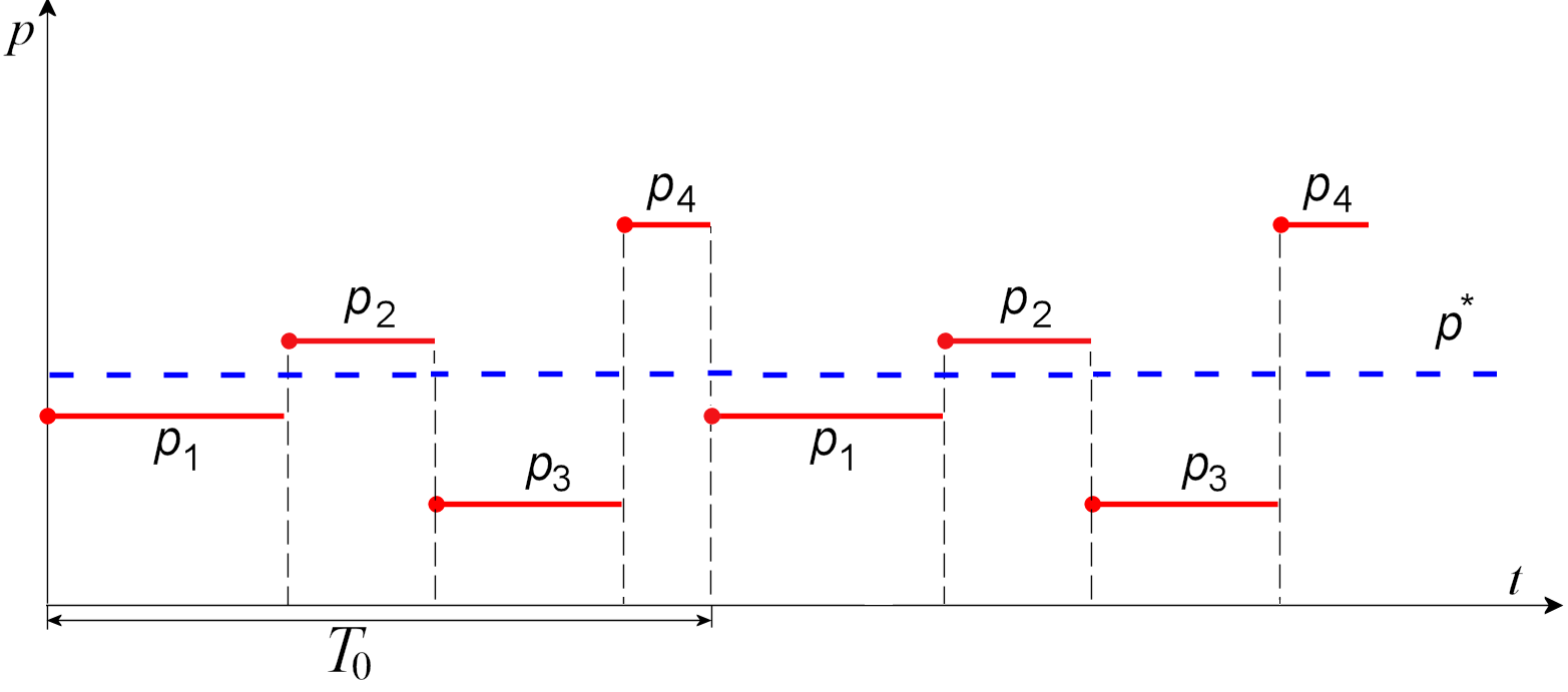
Figure 1: Piecewise constant periodic function $p:I\rightarrow\mathbb{R}$ (sketch).

The control parameter $p$ is considered to be a (periodic) piecewise constant function $p:I\rightarrow\mathbb{R}$ (an example for a periodic function $p$ is presented in Fig.1). As we shall see next, $p$ can be a periodic or non-periodic function. Other form of functions for $p$ can be found in [11].

Due to the piece-wise continuity of $p$, the IVP (1) becomes non-autonomous. However, for the sake of simplicity, next the time variable t will be omitted unless necessary. Therefore, the IVP (1) can be written as follows

$$\frac{{{d^{q}}x}}{{d{t^{q}}}}=f(x)+pBx+Cs(x),\,\,x(0)={x_{0}},\,\,t\in I.$$ (2)

Remark 1.

The existence and uniqueness conditions for IVPs modeling DI and DF systems differ from those for CI systems, and are not presented here (for our class of DI systems they can be found in e.g. [12], while for differential equations of fractional order in [13] or [14].)

The systems chosen to represent in this work the four classes in Table 1 are three-dimensional, but the algorithm and the underlying results are applicable for any finite lower or higher dimension $n$.

The examples treated here are presented in Table 2: Lorenz system, Sprott system [15], Lü system [16] and a fractional variant of the Chua’s system [17]. Other examples can be found in [1, 3, 5, 6, 7].

A global attractor, roughly speaking, is viewed in this paper as a state space region of a dynamical system where the system can enter but not leave, and containing no smaller regions (see e.g. [18]). The global attractor contains all the dynamics evolving from all initial conditions. In other words, it contains all the solutions, including stationary solutions, periodic solutions, as well as chaotic ones. The term of local attractor is used sometimes for attractors which are not global attractors [19].

The global attractors may contain several local attractors. Therefore, a global attractor can be considered as being “composed” of the set of all local attractors for a given parameter $p$ value and initial conditions. Each local attractor attracts trajectories from a subset (basin of attraction) of initial conditions (for details on the notions of local and global attractors we refer e.g. to [20, 21, 22, 23]).

Remark 2.

(i) For the sake of simplicity, when a global attractor is composed by several local attractors, only a single local attractor will be considered (the choice can be made by appropriate selections of the initial conditions). Therefore, hereafter, by attractor one understands, simply, either one of the local attractors or the single local attractor which composes the global attractor;

(ii) Due to the predominant numerical characteristics of the present work, without a significant loss of generality, the attractors will be considered as approximations, after neglecting a sufficiently long period of transients [24], of the $\omega-limit$ sets (the set of points that can be limit of subtrajectories). Despite the fact that usually these sets are uncomputable, they can be numerically approximated. Therefore, in this paper the attractors are considered as being the plots of the $\omega-limit$ sets.

Let us use throughout the review the following notations

Notation 1 - $\mathcal{A}$ the set containing the attractors depending on $p$, including attractive stable fixed points, limit cycles and chaotic attractors;

- $\mathcal{P}$ the set of all p admissible values;

- $\mathcal{P_{N}}=\{p_{1},p_{2},\ldots,p_{N}\}\subset\mathcal{P}$ a finite ordered subset of $\mathcal{P}$;

- $\mathcal{A}_{N}=\{A_{1},A_{2},\ldots,A_{N}\}\subset\mathcal{A}$ the set of the attractors corresponding to $\mathcal{P_{N}};$

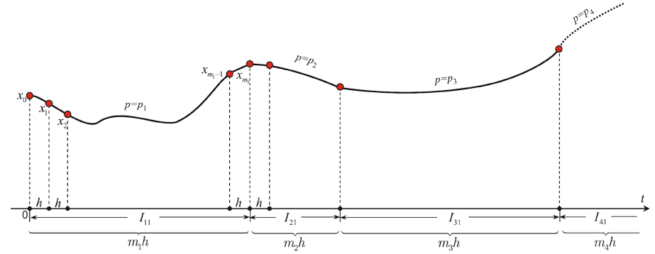
Figure 2: Time subintervals $I_{i1},i=1,2,3$ and $4$ (sketch)

- $I=\bigcup\limits_{j=1,2,\ldots}({\bigcup\limits_{i=1}^{N}{I_{ij}}})$, where the adjoint subintervals $I_{ij}$ are of time length $m_{i}h$, where the ”weights” $m_{i}$ are some positive integers, $h>0$, for $i=1,2,\ldots,N$ and all j (see Fig.2 for the particular case of the first set of time-intervals $I_{i1}$ for $i=1,2,3,4$ );

- $p^{*}$ the average parameter

$${p^{*}}=\frac{{\sum\limits_{i=1}^{N}{{m_{i}}{p_{i}}}}}{{\sum\limits_{i=1}^{N}{{m_{i}}}}};$$ (3)

- $A^{*}$ the average attractor, obtained for $p=p^{*}$.

Remark 3.

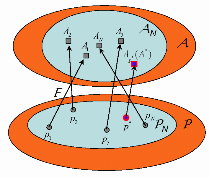
Figure 3: Bijection $F:\mathcal{P}_{N}\rightarrow\mathcal{A}_{N}$ (sketch).

Taking account to the Assumption H1 it follows naturally to define a monotone bijection $F:\mathcal{P}_{N}\rightarrow\mathcal{A}_{N}$ for some fixed N. Therefore, to each $p\in\mathcal{P_{N}}$ corresponds a unique element $A\in\mathcal{A_{N}}$ and reversely, for each $A\in\mathcal{A_{N}}$ there exists $p\in\mathcal{P_{N}}$ such that $A=F(p)$ (Fig.3).

2.2 Parameter Switching algorithm

To prove that any attractor can be approximated by switching the parameter while the underlying IVP is integrated, we need a numerical algorithm to implement the switches that we name Parameter Switching (PS) algorithm.

Let fix for some N, the set $\mathcal{P}_{N}$. Then, ${p^{*}}$ given by (3), can be rewritten in the following form

$${p^{*}}=\sum\limits_{i=1}^{N}{{\alpha_{i}}{p_{i}}}\emph{ with }{\alpha_{i}}={{{m_{i}}}\mathord{\left/{\vphantom{{{m_{i}}}{\sum\limits_{i=1}^{N}{{m_{i}}}}}}\right.\kern-1.2pt}{\sum\limits_{i=1}^{N}{{m_{i}}}}},\,\,{p_{i}}\in{P_{N}}.$$ (4)

Because ${\alpha_{i}}<1$ and $\sum\limits_{i=1}^{N}{{\alpha_{i}}=1}$ , ${p^{*}}$ enjoys the following property

P1. For every set $\mathcal{P}_{N}$, $p^{*}$ given by (3) is a convex combination of $p_{i}$, $i=1,2,\ldots,N$.

To implement the PS algorithm, we have to integrate the IVP (2) with a numerical scheme for ODEs with single step-size h (e.g. the standard Runge-Kutta method).

Let first consider that $p$ is a periodic function of period $T_{0}$, i.e. $p(t+T_{0})=p(t)$ for all $t$ in $I$. While the solution to the IVP (2) is numerically approximated, the parameter p is periodically switched within $\mathcal{P}_{N}$ in every consecutive time interval $I_{ij}$, following some designed scheme, denoted hereafter by $S_{h}$

$$S_{h}\circeq\left[{{p_{1}}\left|{{}_{{I_{1j}}},}\right.{p_{2}}\left|{{}_{{I_{2j}}},\ldots,{p_{N}}\left|{{}_{{I_{Nj}}}}\right.}\right.}\right],\,\,j=1,2,\ldots,$$ (5)

which means that while the IVP (2) is integrated, in each interval ${I_{ij}}$, p will be replaced by $p_{i}$ for every $j=1,2,\ldots$. Thus, for $t\in I_{11}$ , $p(t)=p_{1}$, for $t\in I_{21}$, $p(t)=p_{2}$ and so on until $I_{N1}$, when $p(t)=p_{N}$. On the next interval $I_{12}$, again $p(t)=p_{1}$ and so on until the interval $I_{N2}$, when $p(t)=p_{N}$. The algorithm repeats on the next set of intervals $I_{i3},i=1,2,\ldots,N$ and so on periodically, until $t\geq T$. In other words, $p$ is a piecewise constant and periodic function of period $T_{0}=h\sum\limits_{i=1}^{N}m_{i}$ having the following expression (See Fig.1,2)

$$p(t)={p_{i}},\,\,for\,\,t\in{I_{ij}},\,\,\,i=1,\ldots,N,\,\,\,j=1,2,\ldots$$ (6)

The length of the time intervals $I_{ij}$ will be taken as multiple of h: $length(I_{ij})=m_{i}h$ for each j. Therefore, for a fixed h, $S_{h}$ can be noted in a simplified form

$$S_{h}\circeq\left[{{m_{1}}{p_{1}},{m_{2}}{p_{2}},\ldots,{m_{N}}{p_{N}}}\right],$$ (7)

which means the following p infinite sequence

${m_{1}}{p_{1}},{m_{2}}{p_{2}},\ldots,{m_{N}}{p_{N}},{m_{1}}{p_{1}},{m_{2}}{p_{2}},\ldots,{m_{N}}{p_{N}},\ldots$

For example, $S_{h}=\left[{2{p_{1}},{p_{2}}}\right]$ for a given $h$, means that for the time-interval of length $2h$, $p=p_{1}$ then for the next time-interval of length $h$, $p=p_{2}$ . Next, for two integration steps, $p=p_{1}$, then for one integration step, $p=p_{2}$ and so on

(i.e. periodically with period $T_{0}=(m_{1}+m_{2})h=3h$). Schematically, $\emph{S}_{h}$ can be written as the infinite sequence $\left[{2{p_{1}},{p_{2}}}\right]={p_{1}},{p_{1}},{p_{2}},{p_{1}},{p_{1}},{p_{2}},\ldots$

The pseudocode of the PS algorithm is given in Table 3.

It is easy to verify that

$$p^{\ast}=\frac{1}{T_{0}}\int\limits_{t}^{t+T_{0}}p(\tau)d\tau,~{}~{}t\in I.$$

Notation 2 Let denote by $A^{\circ}$ the attractor, obtained with the PS algorithm, called hereafter the synthesized attractor.

Remark 4.

It is easy to see that, for some given $p$, the relation (3) considered as equation, may have several solutions. For example, if we set $N=2$, and want to obtain $p^{*}=4$ using the scheme $S_{h}=[m_{1}p_{1},m_{2}p_{2}]$, for $p_{1}=2$ and $p_{2}=6$, we can choose $m_{1}=m_{2}=1$ but also $m_{1}=m_{2}=3$ to verify (3). If we fix $m_{1}=3$ and $m_{2}=1$, in order to obtain $p^{*}=4$, we can use $p_{1}=2$ and $p_{2}=10$, but also $p_{1}=p_{2}=4$.

3 Numerical proof of PS algorithm convergence

In this section we prove numerically that for a chosen set of attractors $\mathcal{A}_{N}$, the synthesized attractor $A^{\circ}$ obtained with the PS algorithm belongs to $\mathcal{A}_{N}$ and, moreover, $A^{\circ}$ is approximatively identical to $A^{*}$.

In order to compare two attractors, we have to provide the following criterion

Criterion We shall say that two attractors are approximatively identical (AI) if their trajectories in the phase space approximatively coincide, and the Hausdorff distance (Appendix B) is small enough.

In our numerical experiments Hausdorff distance was of order of $10^{-4}-10^{-3}$.

Due to the bijectivity of F, considering the total order over the set $\mathcal{P}_{N}$, it is reasonable to consider that the following property holds

P2. $\mathcal{A}_{N}$ is an ordered set endowed with the $\mathcal{P}_{N}$ order induced by the function F.

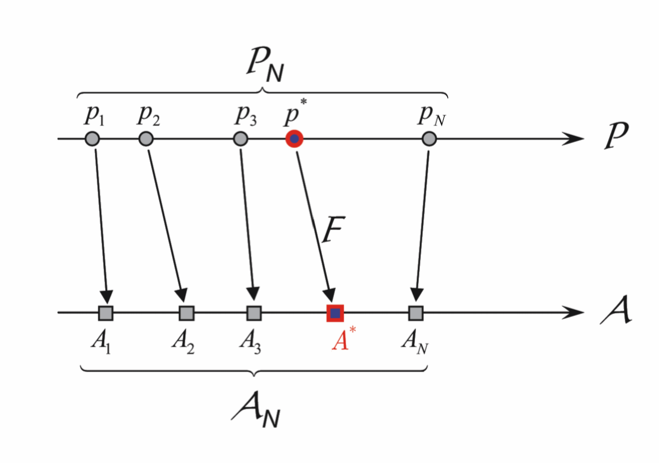
Figure 4: Order induced by $F$ in $\mathcal{A}_{N}$.

Moreover, the same order can be found over the sets $\mathcal{P}_{N}$ and $\mathcal{A}_{N}$ considered as intervals: $\left[{{p_{1}},{p_{N}}}\right]$ and $\left[{{A_{1}},{A_{N}}}\right]$ respectively and, without losing generality, we can consider that ${A_{i}}=F({p_{i}}),\,\,i=1,2,\ldots,N$ (Fig.4). This property is outlined in all bifurcation diagrams.

Notation 3 Let denote AI by $"\cong"$.

Next, in order to prepare the proof of the main result regarding the parameter switching, we introduce the following lemma

Lemma 1.

Given N and $\mathcal{P_{N}}$, $A^{\circ}\cong A^{*}$.

Proof.

The lemma has been checked numerically with tools such as: histograms, Poincaré sections, time series, cross-correlation (Appendix A) and Hausdorff distance (Appendix B). The numerous examples, show that the attractor $A^{\circ}$, obtained with PS algorithm and $A^{*}$ obtained for $p=p^{*}$, are AI, the degree of the identity depending less or more on the system characteristics and, unavoidably, on the numerical errors. Hausdorff distance, for all considered systems, was of order of $10^{-4}-10^{-3}$. ∎

The sketch of the analytical proof of this lemma, presented in [11] for the case of $CI$ systems, can be found in Appendix C.

Remark 5.

Applying the symbolic computation for several examples of CI systems, with the scheme $S_{h}$ for $N\leq 3$, the IVP (2) was integrated with the forward Euler method. The result shown that the (Euclidean) difference between the two solutions corresponding to $p=p^{*}$ and to $p$ switched with the PS algorithm, is of order of $O(h^{2})$, the same as the error of the considered Euler method.

Yet, the main result which can be numerically proved, can be introduced.

Theorem 1.

Given N and $\mathcal{P_{N}}$, $A^{\circ}$ belongs to $(A_{1},A_{N})$.

Proof.

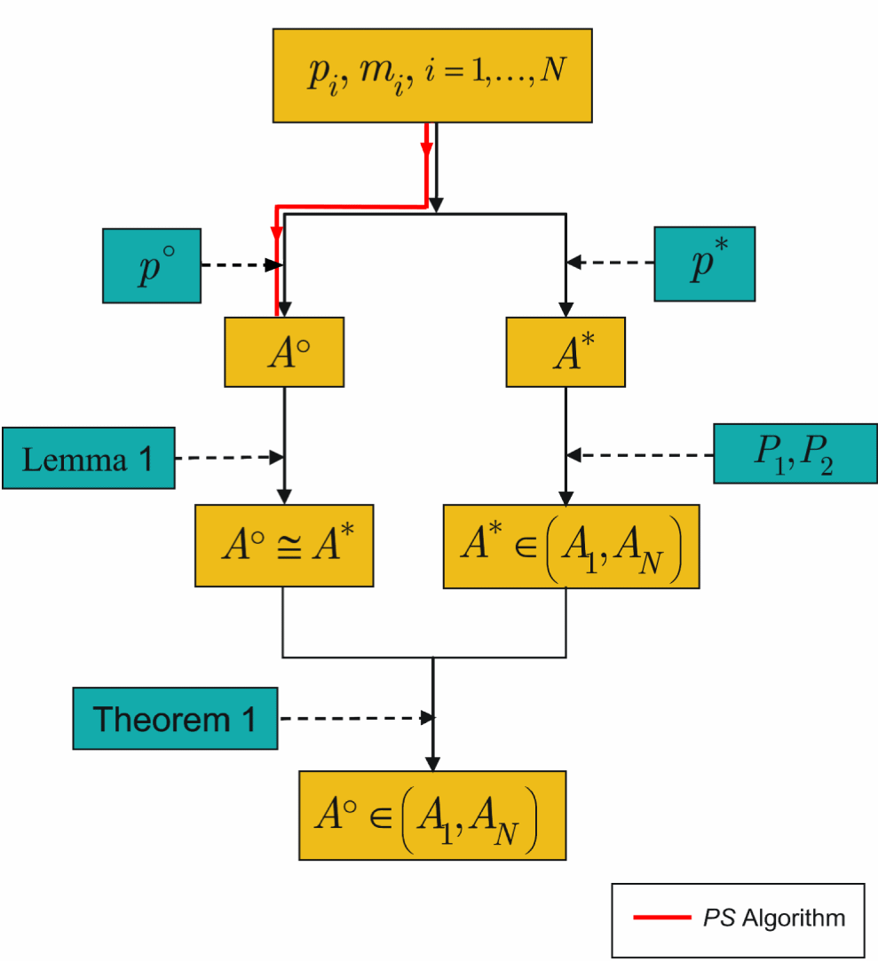
Figure 5: Attractor synthesis: sketch of the proof of Theorem 1.

By the properties P1 and P2, it follows that $A^{*}\in(A_{1},A_{N})$. Next, by the Lemma 1, the attractor $A^{\circ}$ synthesized with some scheme $S_{h}$, is AI to $A^{*}$. Thus, $A^{\circ}\cong A^{*}$ and therefore $A^{\circ}$ belongs to $(A_{1},A_{N})$, which completes the proof (see Fig.5). ∎

Summarizing, for every finite set $\mathcal{P_{N}}$ and numbers $m_{i}$, the synthesized attractor $A^{\circ}$ will belong to $(A_{1},A_{N})$, and differs from every attractor $A_{i}\in\mathcal{A_{N}},\ \ {\it i}=1,2,\ldots N$ (due to the convexity property). Reversely, any attractor of $\mathcal{A_{N}}$ can be considered as being synthesized with the PS algorithm, by means of a finite set of attractors of $\mathcal{A_{N}}$.

For the continuous case, the analytical proof in [11], shows that the solutions of the equation (2) with $p$ switched within $\mathcal{P_{N}}$ with PS algorithm and that with $p$ replaced with $p^{*}$ can be arbitrarily close. Therefore, the underlying invariant sets (attractors in our case) are also arbitrarily (AI) close ([19], Ch. 6).

Due to the mentioned convexity property, whatever kind of combinations of $p_{i}$ and $m_{i}$ values are considered for a fixed $N$, $p^{*}$ will still belong to the interval $(p_{1},p_{N})$. Therefore, for $p$ we can chose any kind of piecewise continuous functions, with the only condition that their values and $p^{*}$ belongs within $\mathcal{P_{N}}$ (see examples in [11]).

The proof of the convergence (analytically or numerically verified) does not depends on the periodicity of $p$ but only on the convexity of $p^{*}$. Therefore, it is obvious that not only periodic schemes (7) can be used, but even random ones [1]. One of the simplest way to implement randomly the PS algorithm, once $N$ is fixed, is to chose first $p_{i}$ and $m_{i}$ in some random manner, after which the PS algorithm is started (see the example of Sprott system, Subsection 4.3). Obviously, there are several other random ways such as: choosing randomly $m_{i}$ and $p_{i}$ while the PS is running, or switching the order of $p_{i}$ and so on. Now, the averaged $p^{*}$ has to be determined with the following relation

$${p^{*}}=\frac{{\sum\limits_{i=1}^{N}{m_{i}^{,}{p_{i}}}}}{{\sum\limits_{i=1}^{N}{m_{i}^{,}}}},\$$ (8)

where $m^{{}^{\prime}}_{i}$ denote the number of times when $p_{i}$ is chosen by the algorithm for $t\in I$.

Remark 6.

(i) The “structural stability” of the $PS$ algorithm presents some obvious limitations due firstly to his numerical approach (some details and other related aspects can be found in [1]). For example, for relative large values of $m_{i}$, the trajectory of $A^{\circ}$ could present some “corners” (a maximum difference between $m_{i}$ should generally be about $(20\div 25)h$). The values for $p_{i}$ could be taken over the entire set $\mathcal{P_{N}}$ without distinguishable differences between $A^{\circ}$ and $A^{*}$. Excessive number of decimals for $p^{*}$ could lead too to some differences between the two attractors $A^{\circ}$ and $A^{*}$. Even for large values for N, $A^{\circ}$ and $A^{*}$ still remain close each other;

(ii) The cross-correlation and time series show an interesting characteristic: the trajectories corresponding to $A^{\circ}$ and $A^{*}$, even in the phase space and time representations are AI, they are dephased in time (see cross-correlation in the figures); (iii) For chaotic attractors, the AI is obtained only “asymptotically” since the necessary time to fully approximate the attractor is, theoretically, infinite.

The PS algorithm can be used to “control” or “anticontrol” dynamical systems modeled by the IVP (2) when some targeted parameter value cannot be accessed directly (see [4]). For this purpose, we have to choose $p_{i}$, $m_{i}$ and some scheme $S_{h}$ to obtain the targeted value $p^{*}$. However, while almost all known control/anticontrol algorithms “force” some trajectory to change its characteristics and behavior, the $PS$ algorithm allows to obtain any desired already existing attractor of $\mathcal{A_{N}}$.

4 Applications

This section is devoted to the applications of the PS algorithm to the four classes of dynamical systems (see Tables 1 and 2) to synthesize attractors. In this purpose we have to choose $N,\mathcal{P_{N}}$ and $S_{h}$ for each system, such that a desired value $p^{*}$ (which can be taken e.g. from the bifurcation diagram) is obtained.

To apply the PS algorithm for CI systems, we used the standard Runge-Kutta method (with the step size $h$ of order between $10^{-4}$ and $10^{-2}$, depending on the characteristics of the considered system), while for the discontinuous and fractional systems, we have chosen special numerical methods. The bifurcation diagrams, time series, histograms and cross-correlations were determined and plotted superimposed for the first state variable $x_{1}$. The Poincaré sections have been determined for the plane $x_{3}=const$. Some bifurcation diagrams, like the one for the Sprott system and especially for the fractional Lü and Chua systems, require an extremely long computer time (see Appendix D ). For discontinuous systems (of integer and fractional order), some ’corners’ can be remarked, typical for these kind of systems (the solution for the underlying IVP are generally not smooth [12, 25]). As stated before, the AI was verified for all the considered systems via superimposed phase portraits, Poincaré sections, histograms, time series and also with cross-correlation and Hausdorff distance. For all the considered cases, the results lead to the same conclusion: Lemma 1 applies to all considered classes of systems.

4.1 Continuous dynamical systems of integer order

The PS algorithm was tested on several examples of CI systems such as: Lorenz, Chen, Rössler, Rabinovitch-Fabrikant [1], Hindmarsh-Rose neuronal system [5], networks [6] and Lotka-Volterra [7]. Here, we consider the representative case of the Lorenz system.

For this class of systems, the IVP (2) has to be considered for the particular case $q=1$ and $C=O_{n\times n}$, namely (Table 2)

$$\dot{x}=f(x)+pBx,\,\,x(0)={x_{0}},\,\,t\in I.$$ (9)

The used numerical method is the standard Runge-Kutta with integration step-size $h=0.01$.

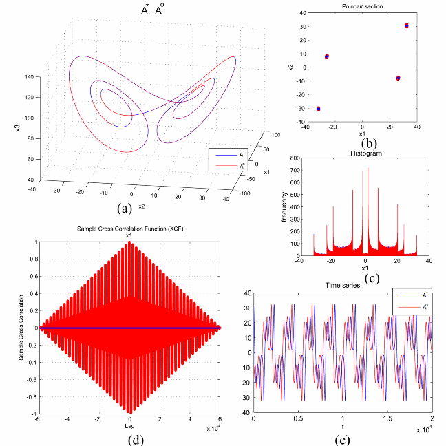
Figure 6: Scheme $[{m_{1}}{p_{1}},{m_{2}}{p_{2}}]$ with $m_{1}=90$, $m_{2}=96$, and $p_{1}=p_{2}=1$ applied to the Lorenz system. $p^{*}=93$. (a) $A^{\circ}$ and $A^{*}$; (b) Poincaré sections; (c) Histograms; (d) Cross-correlations; (e) Time series.

• Let first consider the scheme (7) for $N=2$: $[{m_{1}}{p_{1}},$ ${m_{2}}{p_{2}}]$ with $p_{1}=90$, $p_{2}=96$, and $m_{1}=m_{2}=1$. Then $p^{*}$, given by the relation (3), is $p^{*}=(m_{1}\times p_{1}+m_{2}\times p_{2})/(m_{1}+m_{2})=93$. Applying the PS algorithm, the synthesized attractor $A^{\circ}$ (red plot, Fig.6 a) is a stable limit cycle that is AI with the average attractor $A^{*}$ (superimposed blue plot over $A^{\circ}$) for $p^{*}=93$. The AI is emphasized in addition to the over-plot in the phase space, by the superimposed Poincaré sections with the plane $x_{3}=130$ (Fig.6b) and superimposed histograms for the first state variable $x_{1}$ too (Fig.6c ). The cross-correlation (Fig.6 d) shows that the time series corresponding to $A^{\circ}$ and $A^{*}$ are AI, but dephased. This time-difference between the corresponding trajectories is better remarked from the time series corresponding to the first component $x_{1}$ (see Fig.6 e).

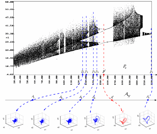
Figure 7: Bifurcation diagram for the Lorenz system.

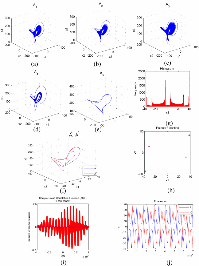
Figure 8: Scheme $\left[{2{p_{1}},3{p_{2}},2{p_{3}},4{p_{4}},3{p_{5}}}\right]$ for $p_{1}=125$, $p_{2}=130$, $p_{3}=140$, $p_{4}=144$ and $p_{5}=220$ applied to the Lorenz system. $p^{*}=154$. (a)-(e) The attractors $A_{i}$ corresponding to $p_{i},i=1,\ldots,5$; (f) $A^{\circ}$ and $A^{*}$; (g) Histograms; (h) Poincaré sections; (i) Cross-correlations; (j) Time Series.

• Let next consider the case $N=5$ with the scheme $\left[{2{p_{1}},3{p_{2}},2{p_{3}},4{p_{4}},3{p_{5}}}\right]$ for $p_{1}=125$, $p_{2}=130$, $p_{3}=140$, $p_{4}=144$ and $p_{5}=220$. In order to facilitate the use of the PS algorithm, the bifurcation diagram will be used (Fig.7). Now, $p^{*}=154$, and the synthesized attractor $A^{\circ}$ is again a stable limit cycle which is AI with $A^{*}$ (Fig.8 f) even $A_{1-4}$ are chaotic and only $A_{5}$ is a stable limit cycle (Fig.8 a-e). Both attractors $A^{\circ}$ and $A^{*}$ are AI (see Fig.8 g-h wherefrom the AI property can be remarked). The time series being dephased (Fig.8 i,j), the trajectories of the attractors $A^{\circ}$ and $A^{*}$ are AI, but time dephased.

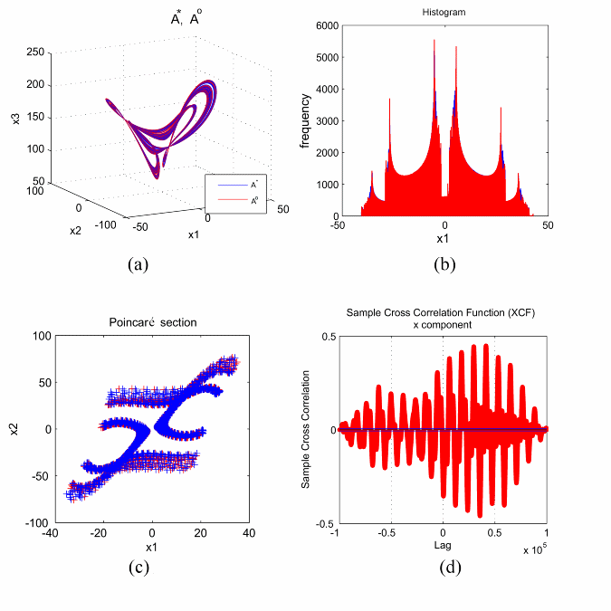
Figure 9: Same scheme as in Fig.8: $\left[{2{p_{1}},3{p_{2}},2{p_{3}},4{p_{4}},3{p_{5}}}\right]$ but with $p_{5}=166$ instead $p_{5}=220$. $p^{*}=142.428$. (a) $A^{\circ}$ and $A^{*}$; (b) Histograms; (c) Poincaré sections; (d) Cross-correlations.

• If for the same scheme $\left[{2{p_{1}},3{p_{2}},2{p_{3}},4{p_{4}},3{p_{5}}}\right]$ we choose $p_{5}=166$ instead $p_{5}=220$, the synthesized attractor $A^{\circ}$ is chaotic and AI with $A^{*}$ for $p^{*}=142.428$ (Fig.9). However, now the AI is only an almost identity (see Remark 6 (iii)). The Poincaré section (Fig.9 c) was obtained with the plane $x_{3}=145$. The cross-correlation shows that the underlying trajectories of $A^{\circ}$ and $A^{*}$ are dephased. Because the trajectories are chaotic, the time series to underline this time-difference is irrelevant in this case.

For all analyzed examples, the Hausdorff distance was of order $10^{-3}$.

Other examples of CI systems can be found in [11].

4.2 Continuous dynamical systems of fractional order

Fractional mathematical concepts allow to describe certain real objects more accurately than the classical “integer” methods. Examples of such real objects that can be elegantly described with the help of fractional derivatives displaying fractional-order dynamics, may be found in many fields of science and exhibit a wide range of rich dynamics. Therefore, the fractional calculus starts to attract increasing attention of mathematicians but also of physicists and engineers (see e.g. [26, 27, 28, 29]).

Many CF systems, can be modeled by the IVP (2) with $q\in(0,1)$ and $C=O_{n\times n}$. The fractional derivative $\frac{{{d^{q}}}}{{d{t^{q}}}}$ is generally denoted using the Caputo differential operator of order q, $D^{q}_{*}$ (see e.g. [30]). Thus, the IVP (2) becomes

$$D^{q}_{*}x=f(x)+pBx,\quad x^{(k)}(0)=x_{0}^{(k)},~{}(k=0,1,\ldots,\lceil q\rceil-1).$$ (10)

$\lceil.\rceil$ denotes the ceiling function that rounds up to the next integer, and $D^{m}_{*}=\frac{d^{m}}{d{t^{m}}}\$, with $m=\lceil q\rceil$, is the standard differential operator of the integer order $\lceil q\rceil\in\mathbb{N}$. The Caputo operator, with starting point 0, has the following expression

$$D^{q}_{*}x(t)=\frac{1}{\Gamma(m-q)}\int_{0}^{t}(t-\tau)^{m-q-1}D^{m}_{*}x(\tau){\mathrm{d}}\tau.$$

where $\Gamma$ is the Gamma function (Appendix D). Because $D^{q}_{*}$ has an m-dimensional kernel, m initial conditions need to be specified. Therefore, for the common case chosen in this paper $0<q<1$, we have to specify just one condition, in the classical form [31]: $x^{\left(0\right)}(0)=x_{0}$.

To implement the PS algorithm in this case, it is necessary to choose a numerical method for the solution to the IVP (10). In this purpose we use the fractional Adams- Bashforth- Moulton method (see Appendix D) introduced in [31].

Let choose for our purpose the fractional variant of the Lü system (see Table 2) which unifies the Lorenz and Chen systems, presented by Lü et al. in [32]. As many of the real fractional systems have the order of the fractional differential operators less than 1, we fix in this paper $q=0.9$ (see [33]) which is a typical value exhibiting all the relevant phenomena (the dynamics of this system, as q varies, can be found in [16], while some aspects of the attractors synthesis of the fractional Lü system is presented in [34]).

Now, the IVP (10) was integrated with the fractional Adams-Bashforth-Moulton method with step size $h=0.005$ and $15000\div 20000$ steps, in function of the dynamics of the synthesized attractor $A^{\circ}$.

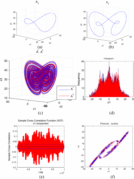
Figure 10: Scheme $[1p_{1},1p_{2}]$ with $p_{1}=32$ and $p_{2}=34.5$ applied to the fractional Lü system. $p^{*}=33.25$. (a),(b) The attractors, $A_{1}$ and $A_{2}$; (c) The attractors $A^{\circ}$ and $A^{*}$; (d) Histograms; (e) Cross-correlations; (f) Poincaré sections.

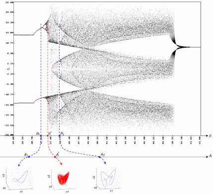
Figure 11: Bifurcation diagram for the Lü system.

• A chaotic attractor $A^{\circ}$ can be obtained with the scheme $[1p_{1},1p_{2}]$ (see Fig.10 c) with $p_{1}=32$ and $p_{2}=34.5$. The attractors corresponding to $p_{1}$ and $p_{2}$ are plotted in Fig.10 a, b which, as can be seen in the bifurcation diagram in Fig.11, are stable limit cycles. $p^{*}=33.25$, and due to the chaotic behavior, the AI between $A^{\circ}$ and $A^{*}$ is only asymptotic (see the histograms in Fig.10 d and the Poincaré sections in Fig.10 f). Even $A^{\circ}$ and $A^{*}$ are chaotic, from the cross-correlation (Fig.10 e), one can see that they are dephased, but still AI.

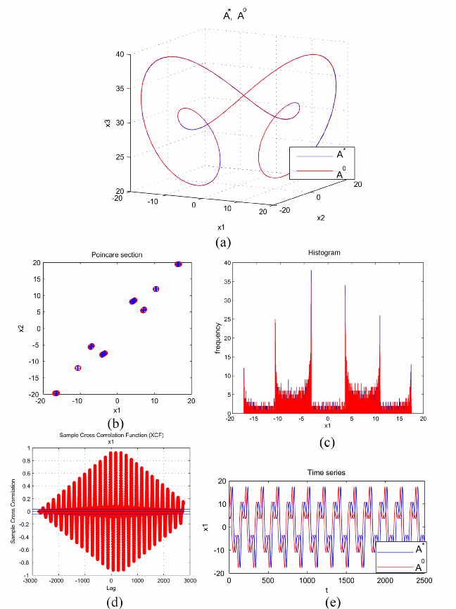
Figure 12: Scheme $[1p_{1},1p_{2}]$, with $p_{1}=33.5$ and $p_{2}=35.5$ for the Lü system. $p^{*}=34.5$. (a) $A^{\circ}$ and $A^{*}$; (b) Poincaré sections; (c) Histograms; (d) Cross-correlations; (e) Time series.

• If we choose the scheme $[1p_{1},1p_{2}]$, with $p_{1}=33.5$ and $p_{2}=35.5$, a stable limit cycle $A^{\circ}$, for which $p^{*}=34.5$, is obtained (Fig.12). The AI can be remarked from the Poincaré section and histograms (Fig.12 b,c). Again, the time difference between the underlying time series can be seen from the cross-correlations (Fig.12 d) and time series (Fig.12 e)

For all tested CF systems, the Hausdorff distance was only of order of $10^{-2}$, compared e.g. with $CI$ systems, where it was of order of $10^{-3}$. This is explainable due to the well known $O(h^{2})$ error bound for the used one-step Adams-Bashforth-Moulton method for fractional systems (detailed discussions on errors can be found in [13]).

4.3 Discontinuous dynamical systems of integer order

Differential equations with discontinuous right-hand side, model a whole variety of realistic applications: dry friction, electrical circuits, oscillations in visco-elasticity, brake processes with locking phase, oscillating systems with viscous dumping, electro-plasticity, convex optimization, control synthesis of uncertain systems and so on (see e.g. [35, 36, 37] and the references therein).

For our class of DI systems, $q=1$ and $C\neq O_{n\times n}$ and the IVP (2) becomes

$$\dot{x}=f(x)+pBx+Cs(x),\,\,\,\,x(0)={x_{0}},\,\,\,t\in I.\$$ (11)

In this case, the right-hand side is discontinuous for a null set of points $M$ where $s$ vanishes, and continuous in $D=\mathbb{R}^{n}\setminus M$. Obviously, the IVP (11) cannot be solved with classical methods. For example, for the equation

$$\dot{x}=2-3{\mathop{\rm sgn}}(x),$$ (12)

where $M=R\backslash({D_{1}}\bigcup{{D_{2}})=\{0\}}$ with $D_{1}=(-\infty,0)$, $D_{2}=(0,\infty)$, the classical solutions, for $x\neq 0$, are

$$x(t)=\left\{\begin{array}[]{l}5t+{C_{1}},\,\,\,x<0,\\ -t+{C_{2}},\,\,x>0,\\ \end{array}\right.$$ (13)

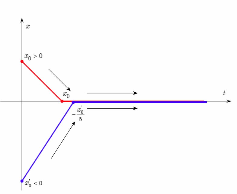
Figure 13: Generalized solutions of the equation (12) (Sketch).

with the integration constants $C_{1},C_{2}$ but, as $t$ increases, these solutions tend to the line $x=0$, where they cannot continue to evolve along this line since the function $x(t)=0$ does not satisfy the equation (Fig.13). Thus, there is no classical solution starting from $0$.

Therefore, the problem has to be restarted as a differential inclusion by using, for example, the Filippov regularization (Appendix E). Thus, the IVP (11) transforms into a differential inclusion (set-valued IVP)

$$\overset{.}{x}\in f(x)+pBx+CS(x),~{}~{}~{}x(0)=x_{0},~{}\text{\emph{for~{}~{}almost~{}all}}~{}~{}t\in I,$$

where $S$ is the setvalued variant of $s$. On mild assumptions, a differential inclusion has a solution that happens to be even unique, but it could have multiple solutions too. To find them numerically, in our particular case of the IVP (11), we can use the standard Runge-Kutta method within $D$ and a special numerical method for differential inclusions in $M$ (the simplest forward Euler method here, see Appendix E).

Once we set the numerical method for the IVP (11), we can apply the PS algorithm. For this class of DI systems, we choose the Sprott system [15] (Table 2).

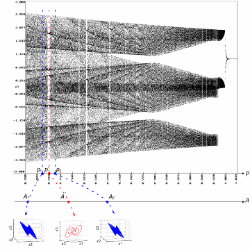
Figure 14: Bifurcation diagram for the Sprott system.

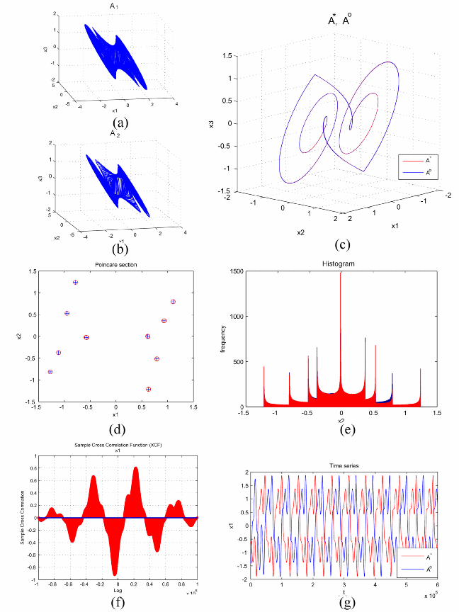
Figure 15: Scheme $[1p_{1},1p_{2}]$ for $p_{1}=0.5$ and $p_{2}=0.528$ applied to the Sprott system. $p^{*}=0.514$. (a),(b) $A_{1}$ and $A_{2}$; (c) $A^{\circ}$ and $A^{*}$; (d) Poincaré sections; (e) Histograms; (f) Cross-correlations; (g) Time series.

• First, let us choose $N=2$ and the scheme $[1p_{1},1p_{2}]$ for $p_{1}=0.5$ and $p_{2}=0.528$, for which the corresponding attractors $A_{1}$ and $A_{2}$ are chaotic (Fig.14). We have chosen this scheme such that the obtained average value $p^{*}=0.514$ belongs to a stable periodic window in the bifurcation diagram. Therefore, the synthesized attractor is a stable limit cycle (Fig.15 c). The AI is underlined by the superimposed Poincaré sections (with the plane $x_{3}=0$, Fig.15 d) and histograms (Fig.15 e). The time-difference between the trajectories is remarked from the cross-correlation (Fig.15 f) and time series (Fig.15 g).

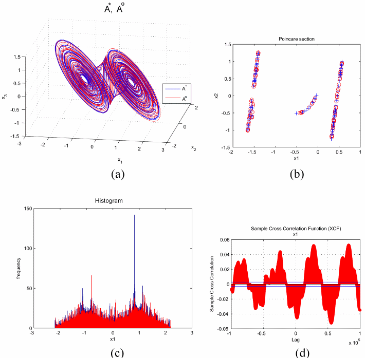
Figure 16: Chaotic PS algorithm applied to Sprott system for $N=100$ and random with uniform distribution choice for $m_{i}$: $m_{i}\in{{1,2,3}}$ and $p_{i}\in[0.45,0.65]$. (a) $A^{\circ}$ and $A^{*}$; (b) Poincaré sections; (c) Histograms; (d) Cross-correlation.

• As seen in Section 3, PS algorithm can be implement in random manners too. For example, for $N=100$ if one choose randomly $m_{i}\in\{1,2,3\}$ and $p_{i}\in[0.45,0.65]$ for $i=1,2,\ldots,100$ with uniform distribution, and with the obtained values we launch PS, the synthesized attractor $A^{\circ}$ is still AI to the average attractor $A^{*}$ (Fig.16). However, taking into account the asymptotic generation of chaotic attractors, and the relative large value for $N$, the small differences between the two attractors, $A^{\circ}$ and $A^{*}$ are explainable.

4.4 Discontinuous dynamical systems of fractional order

There are real discontinuous dynamical systems which display fractional-order dynamics. We consider here the following class of DF systems, modeled by the IVP (2) for $C\neq O_{n\times n}$ and $p<1$

$$\frac{{{d^{q}}x}}{{d{t^{q}}}}=f(x)+pBx+Cs(x),~{}x(0)={x_{0}},~{}t\in I.$$ (14)

In [39] it is proven that the IVP admits solutions which can be numerically determined.

Shortly, the IVP is transformed first into a differential inclusion via the Filippov regularization (as in Subsection 4.3). Next, using the Cellina’s theorem (see e.g. [40, p. 84]) the set-valued IVP of fractional-order is transformed into a continuous single-valued of fractional-order IVP (see for continuous approximation of DI systems the way chosen in [41]). The approximation is made in a sufficiently small $\varepsilon$-neighborhood of the discontinuity points. To be precise, let us consider the simplest example of the scalar function, widely used in examples: $s(x)=c\,sgn(x)$. To approximate $s(x)$ in an $\varepsilon$-neighborhood of $x=0$, we can choose one of the simplest function, the sigmoid $h_{\varepsilon}$

$$h_{\varepsilon}\left(x\right)=c\bigg{(}\frac{2}{1+e^{-x/\varepsilon}}-1\bigg{)}.$$ (15)

For our general case of the IVP (14), the continuous approximation leads to the following continuous IVP of fractional-order

$$\frac{{{d^{q}}x}}{{d{t^{q}}}}-f(x)-pBx=\left\{{\begin{array}[]{*{20}{c}}{Cs(x),\,\,\,for\,\,\,x\notin M,}\\ {{h_{\varepsilon}}(x),\,\,\,\,\,for\,\,\,x\in M,}\\ \end{array}}\right.$$ (16)

where $h_{\varepsilon}(x)$ is the $\varepsilon$-approximation of $Cs(x)$ in the $\varepsilon$-neighborhood of the points $x\in M$, verifying the continuity condition $h_{\varepsilon}(x)=Cs(x)$ on the boundary of the $\varepsilon$-neighborhood [41]. In this way, the discontinuous IVP became a continuous one of fractional order and a numerical scheme for fractional-order differential equations, such as the Adams-Bashforth-Moulton method presented in Subsection 4.2, can be used.

We consider for this case the fractional variant of a discontinuous Chua system presented by [17] (Table 2) for $q=0.98$ (smaller values gives not rich dynamics).

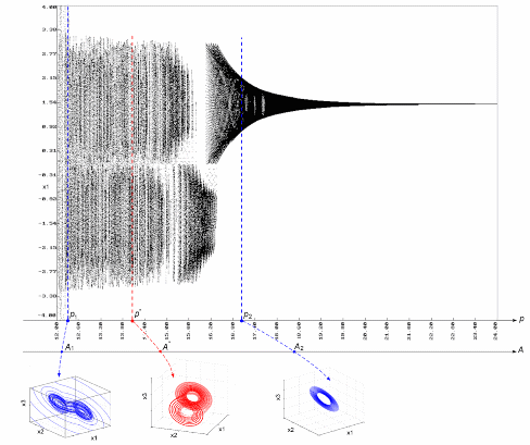
Figure 17: Bifurcation diagram for the fractional Chua system.

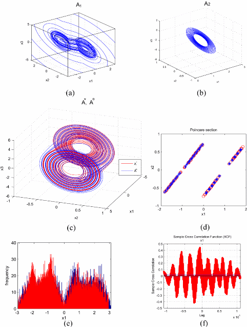
Figure 18: Scheme $[2p_{1},p_{2}]$ with $p_{1}=12.5$ and $p_{2}=17$, applied to the fractional Chua system. $p^{*}=14$. (a),(b) $A_{1}$ and $A_{2}$; (c) $A^{\circ}$ and $A^{*}$; (d) Poincaré sections; (e) Histograms; (f) Cross-correlations.

As it can be seen from the bifurcation diagram (Fig.17), for $p\in(12,12.55)$, there exists a narrow band of a kind of “chaotic saddle”. Within this window, the underlying chaotic attractors look as being “embedded” within this transient chaos (see for example the attractor $A_{1}$ in Fig.18)).

• Using the scheme $[2p_{1},p_{2}]$ with $p_{1}=12.5$ and $p_{2}=17$, the obtained synthesized attractor $A^{\circ}$ is AI with $A^{*}$ for $p^{*}=14$ (Fig.18).

As shown in [33], we found numerically that in these systems of lower than third-order (i.e. $3*q$ which, for $q<1$, is less than 3) chaos still may appear (as it is known, in the case of integer order, according to the well-known Poincaré-Bendixon theorem, chaos appears only at systems of minimum order three).

Conclusions

In this review we have presented the parameter switching algorithm according to which any attractor of a dynamical system belonging to a large class of systems, may be numerically approximated (synthesized). The attractors synthesis is achieved by using the PS algorithm, which switches periodically or randomly the parameter. This facility is enabled by the convexity of $p$. The average and synthesized attractors are AI and their underlying trajectories, time dephased. The review is legitimated by the more than ten published papers each of them containing several applications.

As expected, the performance of the PS algorithm is limited due to the errors of the used numerical method, the length of the time-subintervals $I_{k}$, $k=1,2,...,N$, the number of digits for $p$, the step size $h$ and the distance in the parameter space between $p_{k}$. Thus, we found that $N$ is not a critical parameter (it could be even about $100$). The length of $I_{k}$ (i.e. the value for $m_{k}$) is a critical parameter indicating for how long time the control parameter of the considered system can take the values $p=p_{k}$. We found that a maximum value for $m_{k}$ can be taken about $25h$. For $p$, $3-4$ digits are enough to be compatible with the smallest distance between the $p_{k}$ in the bifurcation diagrams. Moreover, some real physical chaotic systems may have an infinite number of different states or limit cycles with infinite period. But a computer simulated system has a finite number of states; if the precision of the computer is $n$ bits and the system to be modeled has $k$ variables, the total number of system states is limited to $2^{k*n}$; hence, given a determined state, it will be repeated sooner or later and the system will become periodic, with a period equal to the separation of the two occurrences of the state. The PS method can alleviate this inaccuracy and make possible the approximation of a computer simulated system to a real one, although it may be necessary to use a sequence of parameter values lasting as the whole segment of the system to be modeled (se e.g. [42]).

Some open problems are: the analytical proofs for the Lemma 1 for CF, DI and DF systems, not only for CI as done in [11]; an analytical proof for the continuity of the bijection $F$; a detailed study of the time delay between the trajectories of $A^{\circ}$ and $A^{*}$; the effect of noise on the results; a comparison with the complex systems (fractals), where the parameter switching may lead also to some interesting results [8].

APPENDIX

Appendix A Cross Correlation

As known, the cross-correlation of two signals is a measure of the similarity of two waveforms. The cross-correlation has ranges from -1.0 to +1.0. The closer it is to $+1$ or $-1$, the more closely the two compared variables are related. The correlation of two signals (the attractors underlying trajectories in our case) may indicate that one of them is delayed in time with respect to the other. The maximum value (close to unity) of this cross-correlation is obtained when the two signals are in closest alignment with each other. The value $-1$ means the signals are identically matched but opposite in phase, while a value approaching zero indicates a low degree of similarity (see the blue band around the horizontal axe in our images). In this paper, the results were obtained with the crosscorr Matlab function with approximate $95$ percent confidence interval.

Appendix B Hausdorff distance

The Hausdorff distance in a metric space, measures how far two compact nonempty subsets are from each other. The classical Hausdorff distance between two (finite) sets of points, A and B, is defined as [43, p.114]

$${D_{H}}(A,B)=\max\left\{{\mathop{\sup}\limits_{x\in A}\mathop{\inf}\limits_{y\in B}d(x,y),\mathop{\sup}\limits_{y\in B}\mathop{\inf}\limits_{x\in A}d(x,y)}\right\},\$$

where $d(x,y)$ is the classical distance between two points in the considered space.

If the two sets are curves, $D_{H}$ is defined as the maximum distance to the closest point between the curves. Thus, if the curves are defined as the sets of ordered pair of coordinates $A=\{a_{1},a_{2},\ldots,a_{n}\}$ and $B=\{b_{1},b_{2},\ldots,b_{m}\}$ the distance to the closest point between a point $a_{i}$ to the set B is

$$d({a_{i}},B)=\mathop{\min}\limits_{j}\left\|{{b_{j}}-{a_{i}}}\right\|.$$

Thus, the Hausdorff distance is

$${d_{H}}(A,B)=\max\left\{{\mathop{\max}\limits_{i}\left\{{d({a_{i}},B)}\right\},\mathop{\max}\limits_{j}\left\{{d({b_{j}},A)}\right\}}\right\}.\$$

Appendix C Sketch of the analytical proof of Lemma 1

Next, the main steps of the proof presented in [11] for the lemma, ensuring the AI between $A^{\circ}$ and $A^{*}$ in the case of CI systems, are pointed out.

Consider the IVP (1) with $C=O_{n\times n}$ and $q=1$ satisfying the assumptions stated in Section 2 and expressed for the general case of $\mathbb{R}^{n}$, in the following form

$$\dot{x}(t)=f(x(t))+p\left(t/\lambda\right)Bx(t),~{}x(0)=x_{0},t\in I=[0,\infty),$$ (17)

where $\lambda\in\mathbb{R}_{+}^{*}$ is a positive real number which will be stated later, and $p:I\rightarrow\mathbb{R}^{n}$ is considered as a piecewise continuous periodic function with period $T_{0}$, and mean value $q$, i.e.

$$\frac{1}{T_{0}}\int_{t}^{t+T_{0}}p(u)du=q,~{}t\in I.$$

Let us define the average model of (17) obtained with the PS algorithm, expressed as follows

$$\dot{y}=f(y)+qBy,~{}y(0)=y_{0}.$$ (18)

The IVP (17) models the PS algorithm and generates the synthesized attractor $A^{\circ}$, while the IVP (18) represents the system whose solution approximates the average attractor $A^{*}$.

We have to prove that the solutions of the equations (17) and (18) differ by less than $\lambda^{2}$ for $\lambda$ sufficiently small, via the so called order function defined in terms of approximations.

Let next suppose that (18) satisfies the assumption H1 and admits $s:I\rightarrow\mathbb{R}$ as the unique solution.

Linearizing (18) on a neighborhood of $s$, one obtains the following IVP

$$\dot{\varepsilon}(t)=[E(t)+qB]\varepsilon(t),\qquad\varepsilon(0)=\varepsilon_{0},$$ (19)

where $\varepsilon(t)=y(t)-s(t)$ and $E(t)$ denotes the Jacobian of $f$ evaluated at $s(t)$.

Because $s(t)$ is the solution in (18), $\varepsilon(t)=0$ for $t\in I$, should be a solution of (19).

If we linearize the IVP (17) for $x\in\Gamma_{s}$ (the domain of attraction of $\varepsilon=0$) one obtains

$$\dot{e}(t)=[E(t)+p(t/\lambda)B]e(t),\qquad e(0)=e_{0},$$

where $e(t)=x(t)-s(t)$.

Then, the theorem ensuring the AI between the attractors of the dynamical system modeled by the IVP (17) and IVP (18) can be enounced.

Theorem Let assume that Eq. (19) is uniformly exponentially stable, i.e. there exist the constants $K>0,\mu>0$ such that

$$\varepsilon(t)\leq K||\varepsilon_{0}||\exp(-\mu t).$$

Then, for $e_{0}=\varepsilon_{0}$, there exists a positive scalar $\lambda>0$, such that $\lim_{t\rightarrow\infty}||e(t)-\varepsilon(t)||=\delta(\lambda^{2})$, where $\delta(\lambda^{2})$ is an order function.

Proof.

The complete proof can be found in [11] and it mainly follows the idea given in Chapter 4 of [44]. The existence interval $I$ is partitioned as follows: $I=\left[0,\lambda T\right]\bigcup\left[\lambda T_{0},2\lambda T_{0}\right]\cdots$. In each subinterval $I_{n}=\left[n\lambda T_{0},(n+1)\lambda T_{0}\right],n=1,2,\ldots$, Eq. (19) has the solution $\varepsilon_{n}(t)$. If on these subintervals, the initial condition is chosen $\varepsilon_{n}(n\lambda T_{0})=e(n\lambda T_{0})$, using a generalized Peano-Baker series [45], the Gronwall’s inequality, through straightforward algebraic operations, the following inequality is inductive proved

$$||e((n+1)\lambda T_{0})-\varepsilon_{n}((n+1)\lambda T_{0})||\leq\delta(\lambda^{2}),$$

for any $n$. Taking the limit $n\rightarrow\infty$, the proof is complete. ∎

Appendix D Adams-Bashforth-Moulton scheme for fractional ODEs

Next, a brief presentation of the Adams-Bashforth-Moulton scheme [31] is presented. Let consider the IVP (10). Specifically, the method implies a discretization of $I$ with grid points $t_{i}=hi,\ \ i=0,1,\ldots$ with a preassigned step size h. First, a preliminary approximation $x_{i+1}^{\mathrm{P}}$ for $x(t_{i})$ (the predictor phase) is computed via the formula

$$x_{i+1}^{\mathrm{P}}=\sum_{j=0}^{\lceil q\rceil-1}\frac{t_{i+1}^{j}}{j!}x_{0}^{(j)}+\frac{1}{\Gamma(q)}\sum_{j=0}^{i}b_{j,i+1}g(x_{j}),$$

where $b_{j,i+1}$ have the form

$$b_{j,i+1}=\frac{h^{q}}{q}\left((i+1-j)^{q}-(i-j)^{q}\right).$$

Then, the final approximation $x_{i+1}$ for $x(t_{i+1})$ (the corrector phase) is

$$x_{i+1}= \sum_{j=0}^{\lceil q\rceil-1}\frac{t_{i+1}^{j}}{j!}x_{0}^{(j)}+\frac{h^{q}}{\Gamma(q+2)}\left(\sum_{j=0}^{i}a_{j,i+1}g(x_{j})+g(x_{i+1}^{\mathrm{P}})\right),$$

with

$$a_{0,i+1}=i^{q+1}-(i-q)(i+1)^{q},$$

and

$$a_{j,i+1}=(i-j+2)^{q+1}+(i-j)^{q+1}-2(i-j+1)^{q+1},$$

for $j=1,2,\ldots,i$.

The Gamma function, $\Gamma$, is approximated in this work with the so-called Lanczos approximation [46]

$$\Gamma(z)=\frac{\sum_{i=0}^{6}p_{i}z^{i}}{\prod_{i=0}^{6}(z+i)}(z+5.5)^{z+0.5}{\mathrm{e}}^{-(z+5.5)}.$$

for $z\in\mathbb{C}$ with $\mathop{\mathrm{Re}}(z)>0$. The coefficients $p_{i}$ are shown in Table 4.

While in the standard methods for ODEs of integer order, the current approximation $x_{k}$ depends only on the results of a few backward steps, like all reasonable numerical methods for fractional differential equations, the fractional scheme Adams-Bashforth-Moulton requires the entire backward integration history at each point in time. Thus, each calculated value $x_{k}$ depends on all previous values $x_{0},x_{1},\ldots,x_{k-1}$. This characteristic implies a serious drawback with respect to the required computing time. For example, to obtain $4000$ points within some attractor, about $8\times 10^{6}$ iterations are necessary. However, this is necessary to appropriately reflect the memory effects possessed by fractional differential operators.

A detailed analysis of this method can be found in [13] and a background on fractional differential equations is presented in [14].

Appendix E Filippov regularization

Let consider the following general IVP with discontinuous right-hand side

$$\dot{x}=f(x),\,\,\,\,x(0)={x_{0}},\,\,\,t\in I,$$ (20)

with $f$ locally bounded on $\mathbb{R}^{n}$. In particular, the discontinuity is due to the discontinuity of the state variable, of the associated vector field, of Jacobian (partial derivatives) or higher order discontinuity. The continuity domain consists in a finite $m$ number of open regions ${D_{i}}\subset{\mathbb{R}^{n}},\,\,\,i=1,2,\ldots,m$, the discontinuity set $M$ being $M$ = ${\mathbb{R}^{n}}\backslash\bigcup\nolimits_{i=1}^{m}{{D_{i}}}$.

The IVP (20) may have not any solutions in the classical sense. Therefore, in this paper we have chosen the way given by [47], which transforms the IVP (20), via the differential inclusion approach, into a multi-valued Cauchy IVP

$$\dot{x}\in F(x),\,\,\,\,x(0)={x_{0}},\,\,\,\,for~{}almost~{}all~{}t\in I,$$ (21)

where, $F:\mathbb{R}^{n}\rightrightarrows\mathbb{R}^{n}$ is a set-valued function into the set of all subsets of $\mathbb{R}^{n}$. For our class of systems, F can be defined using the so called Filippov regularization

$$F(x)=con\mathop{\lim}\limits_{x^{\prime}\to x}f(x^{\prime}),$$

where $con$ means the convex hull and $\lim_{x^{\prime}\to x}f(x^{\prime})$ represents the set of all limits for all convergent sequences $f(x_{k})$ with $x_{k}\rightarrow x$. For $x\in M$, $F(x)$ is a set, while for $x\notin M$, $F(x)$ consists in a single point $f(x)$. As example, for the sign function the Filippov regularization gives the following set-valued function

$$\ Sgn(x)=\left\{{\begin{array}[]{*{20}{c}}{\{-1\},\,\,x<0,}\\ {[-1,1]\,\,\,\,x=0,}\\ {\{+1\}\,\,\,\,\,\,x>0.}\\ \end{array}}\right.\$$

For example, the Filippov regularization applied to the Example (12) leads to the following differential inclusion

$$\dot{x}\in 2-3{\mathop{\rm Sgn}}(x).$$ (22)

Definition [47] A generalized solution (or Filippov solutions) of the IVP (20) is an absolutely continuous vector-valued function $x:I\to{R^{n}}$ verifying the IVP (21) for a.a. $t\in I$.

Even the IVP (20) may have no classical solutions, the setvalued IVP (21) may have a unique or several generalized solutions. For example, the equation (12), after regularization becomes the set-valued problem (22) and has the following generalized solutions: if $x_{0}>0$, then $x(t)=-t+x_{0}$ for $t<x_{0}$ and $x(t)=0$ for $t\geq x_{0}$. In other words, the solution can be prolonged continuous along the axis $x=0$. If $x^{\prime}_{0}<0$, the solution is $x(t)=5t+x^{\prime}_{0}$ for $t<x^{\prime}_{0}$ and $x(t)=0$ for $t\geq x^{\prime}_{0}$ (Fig.13)

The background of differential inclusions and their solutions can be found e.g. in [40] and [48]. The existence and uniqueness of solutions for our class of DI systems are presented in [49] and will be not considered here.

To solve numerically the IVP (20) special numerical methods for differential inclusions are necessary. However, for our class of IVPs, due to the presence of $s$ functions, the discontinuity appears only in a finite null set M, where actually the IVP is a set-valued problem. For the points $x\in{D_{i}}$, the IVP is a continuous problem. Therefore, we can integrate in $D_{i}$ the IVP (20) using e.g. the standard Runge-Kutta method, while for $x\in M$, a numerical method for the corresponding differential inclusion $\dot{x}\in F(x)$ has to be used. Precisely, when the trajectory enters the discontinuity surface, we have to choose for derivative of solution, generally for some finite time, a value within the set $F(x)$ while a numerical method for differential inclusions is used (the simplest one is the adapted forward Euler method see e.g. [12, 25]). For example, when $x=0$ in the Example (12), we have to solve the differential inclusion $\dot{x}\in[-1,5]$. There are several possibilities to manage this problem using e.g. so called selection strategies (see [50]). In this paper we used the simplest way, namely the random strategy which implies a randomly choice of a value within $F(x)$ (the interval $[-1,5]$ in our example). There are several possibilities to find the moments when the trajectory enters and leaves the discontinuity surfaces (see e.g. [37]) during which the chosen method solves the differential inclusion.

Table 1: Classification of the considered dynamical systems modeled by the IVP (1).

	$C={0_{n\times n}}$	$C\neq{0_{n\times n}}$
$q=1$	Continuous of Integer order (CI) systems	Discontinuous of Integer order (DI) systems
$q\in(0,1)$	Continuous of Fractional order (CF) systems	Discontinuous of Fractional order (DF) systems

Table 2: Systems utilized in this paper.

Type	Order	System	$q$	$f(x)$	$B$	$C$
Continuous	Integer	Lorenz $\dot{x}_{1}=10(x_{2}-x_{1})$ $\dot{x}_{2}=-x_{1}x_{3}-x_{2}+px_{1}$ $\dot{x}_{3}=x_{1}x_{2}-\frac{8}{3}x_{3}$	$1$	$\left(\begin{array}[c]{c}{10(x}_{2}{-x}_{1}{)}\\ {-x}_{1}{x}_{3}{-x}_{2}\\ {x}_{1}{x}_{2}{-}\frac{8}{3}{x}_{3}\end{array}\right)$	$\left(\begin{tabular}[c]{lll}$0$&$0$&$0$\\ $1$&$0$&$0$\\ $0$&$0$&$0$\end{tabular}\right)$	$O_{3\times 3}$
Continuous	Fractional	Lü $\frac{d^{q}x_{1}}{dt^{q}}=-x_{1}+px_{2}$ $\frac{d^{q}x_{2}}{dt^{q}}=-x_{1}x_{3}+28x_{2}$ $\frac{d^{q}x_{3}}{dt^{q}}=x_{1}x_{2}-3x_{3}$	$q<1$	$\left(\begin{array}[c]{c}{\-x}_{1}\\ {-x}_{1}{x}_{3}{+28x}_{2}\\ {x}_{1}{x}_{2}{-3x}_{3}\end{array}\right)$	$\left(\begin{tabular}[c]{lll}$0$&$1$&$0$\\ $0$&$0$&$0$\\ $0$&$0$&$0$\end{tabular}\right)$	$O_{3\times 3}$
Discontinuous	Integer	Sprott $\dot{x}_{1}=x_{2}$ $\dot{x}_{2}=x_{3}$ $\dot{x}_{3}=-x_{1}-x_{2}-px_{3}+sgn(x_{1})$	$1$	$\left(\begin{array}[c]{c}{x}_{2}\\ {x}_{3}\\ {-x}_{1}{-x}_{2}\end{array}\right)$	$\left(\begin{tabular}[c]{lll}$0$&$0$&$0$\\ $0$&$0$&$0$\\ $0$&$0$&$-1$\end{tabular}\right)$	$\left(\begin{tabular}[c]{lll}$0$&$0$&$0$\\ $0$&$0$&$0$\\ $1$&$0$&$0$\end{tabular}\right)$
Discontinuous	Fractional	Chua $\frac{d^{q}x_{1}}{dt^{q}}=-2.57x_{1}+9x_{2}+3.86sgn(x_{1})$ $\frac{d^{q}x_{2}}{dt^{q}}=x_{1}-x_{2}+x_{3}$ $\frac{d^{q}x_{3}}{dt^{q}}=-px_{2}$	$q<1$	$\left(\begin{array}[c]{c}{-2.57x}_{1}{+9x}_{2}\\ {-x}_{1}{-x}_{2}{+x}_{3}\\ {0}\end{array}\right)$	$\left(\begin{tabular}[c]{lll}$0$&$0$&$0$\\ $0$&$0$&$0$\\ $0$&$-1$&$0$\end{tabular}\right)$	$\left(\begin{tabular}[c]{lll}$3.86$&$0$&$0$\\ $0$&$0$&$0$\\ $0$&$0$&$0$\end{tabular}\right)$

Table 3: Pseudo-code of the PS algorithm

CHOOSE $S_{h}$, T, h

REPEAT

FOR $i=1$ to $N$

FOR $k=1$ to $m_{i}$

one step integration of the IVP (2) for $p=p_{i}$

$\ \ \ \ \ \ \ \ \ \ \ \ \ \ \ \ \ \ \ \ \ t=t+h$

ENDFOR

ENDFOR

UNTIL $t\geq T$

Table 4: Coefficients of the Lanczos approximation.

$i$	$p_{i}$
$0$	${75122.6331530}$
$1$	${80916.6278952}$
$2$	${36308.2951477}$
$3$	${8687.2452971}$
$4$	${1168.9264948}$
$5$	${83.8676043}$
$6$	${2.5066283}$

References

- [1] Danca, M.-F., Tang W.K.S., Chen, G.: A switching scheme for synthesizing attractors of dissipative chaotic systems. Applied Mathematics and Computation 201, 1–2 (2008)
- [2] Danca, M.-F.: Random parameter-switching synthesis of a class of hyperbolic attractors. Chaos 18, 033111 (2008)
- [3] Danca, M.-F.: Synthesizing the Lü attractor by parameter-switching. Int. J. Bifurcation and Chaos 21(1), (2011)
- [4] Danca, M.-F.: Finding stable attractors of a class of dissipative dynamical systems by numerical parameter switching. Dynamical Systems 25(2), 189–201 (2010)
- [5] Danca, M.-F., Wang, Q.: Synthesizing attractors of Hindmarsh-Rose neuronal systems. Nonlinear Dynamics 62(1), 437–446 (2010)
- [6] Danca, M.-F., Morel, C.: Attractors synthesis of a class of networks. Dynamics of Continuous, Discrete & Impulsive Systems B, accepted (2010)
- [7] Danca, M.-F.: Attractors synthesis for a Lotka-Volterra-like system. Applied Mathematics and Computation 216, 2107–2117 (2010)
- [8] Almeida, J., Peralta-Salas, D., Romera, M.: Can two chaotic systems give rise to order?. Physica D 200, 124–132 (2005)
- [9] Romera, M., Small, M., Danca, M.-F.: Deterministic and random synthesis of discrete chaos. Applied Mathematics and Computation 192(1), 283–297 (2007)
- [10] Danca, M.-F., Romera, M., Pastor, G.: Alternated Julia sets and connectivity properties. Int. J. Bifurcat. Chaos 19, 2123–2129 (2009)
- [11] Mao, Y., Tang, W.K.S., Danca, M.-F.: An Averaging Model for the Chaotic System with Periodic Time-Varying Parameter. Applied Mathematics and Computation 217(1), 355 362 (2010)
- [12] Lempio, F.: Difference methods for differential inclusions. Lect Notes Econ. Math. Syst. 378, 236–273 (1992)
- [13] Diethelm, K., Ford, N.J., Freed, A.D.: Detailed error analysis for a fractional Adams method. Numer. Algorithms 36, 31–52 (2004)
- [14] Diethelm, K.:The Analysis of fractional differential equations An application-oriented exposition using differential operators of Caputo type. Springer, Berlin Heidelberg (2010)
- [15] Sprott, J.C.: A new class of chaotic circuit. Phys. Lett. A 266, 19–23 (2000)
- [16] Lü, J.G.: Chaotic dynamics of the fractional-order L system and its synchronization. Physics Letters A 354, 305–311 (2006)
- [17] Brown, R.: Generalizations of the Chua equations. IEEE Trans. Circuits Syst.-I: Fund. Th. Appl. 40(11), 878–883 (1993)
- [18] Kapitanski, L., Rodnianski, I.: Shape and Morse theory of attractors. Communications on Pure and Applied Mathematics 53, 218–242 (2000)
- [19] Stuart, A., Humphries, A. R.: Dynamical systems and numerical analysis. Cambridge Monographs on Applied and Computational Mathematics (No. 2). Cambridge University Press, Cambridge (1998)
- [20] Milnor, J.: On the concept of attractor. Communications in Mathematical Physics 99, 177–195 (1985)
- [21] Temam, R.: Infinite dimensional dynamical systems in mechanics and physics. Applied Mathematical Sciences 68, Springer-Verlag, New York (1988)
- [22] Hirsch, W.M., Pugh, C.: Stable manifolds and hyperbolic sets. in: Proc. Symp. Pure Math., 14, American Mathematical Society, 133–164 (1970)
- [23] Hirsch, W.M., Smale, S., Devaney, L. R.: Differential Equations, Dynamical Systems and An Introduction to Chaos, second ed. Elsevier Academic Press, London (2004)
- [24] Foias, C., Jolly, M. S.: On the numerical algebraic approximation of global attractors. Nonlinearity 8, 295–319 (1995)
- [25] Lempio, F.: Euler’s method revisited. Proc. Steklov Institute of Mathematics Moscow 211, 473–494 (1995)
- [26] Podlubny, I.: Fractional Differential Equations. Academic Press, New York (1999)
- [27] Hilfer, R. (Ed.): Applications of Fractional Calculus in Physics. World Scientific, New Jersey (2000)
- [28] Ahmed, E., Elgazzar, A.S.: On fractional order differential equations model for nonlocal epidemics. Physica A 379, 607–614 (2007)
- [29] El-Sayed, A.M.A. El-Mesiry, A.E.M., El-Saka, H.A.A.: On the fractional-order logistic equation. Applied Mathematics Letters 20, 817–823 (2007)
- [30] Podlubny, I., Petrás, I., Vinagre, B.M., O’Leary, P., Dorcák, L.: Analogue realization of fractional-order controllers. Nonlinear Dynamics 29, 281–296 (2002)
- [31] Diethelm, K., Ford, N. J., Freed, A.D.: A predictor-corrector approach for the numerical solution of fractional differential equations. Nonlinear Dynamics 29, 3–22 (2002)
- [32] Lü, J., Chen, G., Cheng, D., Celikovsky, S.: Bridge the gap between the Lorenz system and the Chen system. Int. J. Bifurcation Chaos 12, 2917–2926 (2002)
- [33] Danca, M.-F.: Chaotic behavior of a class of discontinuous dynamical systems of fractional-order. Nonlinear Dynamics 60(4), 525–534 (2010)
- [34] Danca, M.-F., Diethlem K.: Fractional-order attractors synthesis via parameter switchings. Communications in Nonlinear Science and Numerical Simulations 15(12), 3745–3753 (2010)
- [35] Popp, K., Stelter, P.: Stick-slip vibrations and chaos. Philos. Trans. R. Soc. London A 332, 89–105 (1990)
- [36] Deimling, K.: Multivalued differential equations and dry friction problems. Proc. Conf. Differential & Delay Equations, Ames, Iowa, eds. Fink, A. M., Miller, R. K. & Kliemann, W. World Scientific, 99–106 (1992)
- [37] Wiercigroch, M., de Kraker, B.: Applied Nonlinear Dynamics and Chaos of Mechanical Systems with Discontinuities. World Scientific, Singapoore (2000)
- [38] Danca, M.-F.: On a class of non-smooth dynamical systems: a sufficient condition for smooth vs nonsmooth solutions. Regular & Chaotic Dynamics 12(1), 1–11 (2007)
- [39] Danca, M.-F.: Numerical Approximation of a Class of Discontinuous Systems of Fractional Order. Nonlinear Dynamics, accepted, 2010, DOI: 10.1007/s11071-010-9915-z
- [40] Aubin, J.-P., Cellina, A.: Differential inclusions set-valued maps and viability theory. Springer Verlag, Berlin (1984)
- [41] Danca, M.-F., Codreanu, S.: On a possible approximation of discontinuous dynamical systems. Chaos, Solitons & Fractals 13(4), 681–691 (2002)
- [42] Li, S., Chen, G., Mou, X.: On the dynamical degradation of digital piecewise linear chaotic maps. International journal of Bifurcation and Chaos 15, 3119–3151 (2005)
- [43] Falconer, K.: Fractal Geometry: Mathematical Foundations and Applications. John Wiley & Sons, Chichester (1990)
- [44] Sanders, J.A., Verhulst, F.: Averaging Methods in Nonlinear Dynamical Systems. Springer-Verlag, New York (1985)
- [45] Dacunha, J.J.: Transition matrix and generalized matrix exponential via the Peano-Baker Series. Journal of Difference Equations and Applications 11(15), 1245–1264 (2005)
- [46] Press, W. H., Teukolsky, S.A., Vetterling, W. T., Flannery, B.P.: Numerical Recipes in C: The Art of Scientific Computing, 2nd ed. Cambridge University Press, Cambridge (1992)
- [47] Filippov, A.F.: Differential equations with discontinuous righthand sides. Kluwer Academic Publishers, Dordrecht (1988)
- [48] Aubin, J.-P., Frankowska, H.: Set-valued analysis. Birkhäuser, Boston (1990)
- [49] Danca, M.-F.: On a class of discontinuous dynamical system. Miskolc Mathematical Notes, 2(2), 103–116 (2001)
- [50] Kastner-Maresch, A., Lempio, F.: Difference methods with selection strategies for differential inclusions. Numer. Funct. Anal. Optim. 14(5–6), 555–572 (1993)