The merging cluster Abell 1758 revisited: multi-wavelength observations and numerical simulations

Abstract

Context. We discuss here the properties of the double cluster Abell 1758, at a redshift z$\sim$0.279, which shows strong evidence for merging.

Aims. We analyse the optical properties of the North and South clusters of Abell 1758 based on deep imaging obtained with the CFHT archive Megaprime/Megacam camera in the $g^{\prime}$ and $r^{\prime}$ bands, covering a total region of about 1.05$\times$1.16 deg², or $16.1\times 17.6$ Mpc². Our X-ray analysis is based on archive XMM-Newton images. Numerical simulations were performed using an N-body algorithm to treat the dark matter component, a semi-analytical galaxy formation model for the evolution of the galaxies and a grid-based hydrodynamic code with a PPM scheme for the dynamics of the intra-cluster medium. We have computed galaxy luminosity functions (GLFs) and 2D temperature and metallicity maps of the X-ray gas, which we then compared to the results of our numerical simulations.

Methods. The GLFs of Abell 1758 North are well fit by Schechter functions in the $g^{\prime}$ and $r^{\prime}$ bands, but with a small excess of bright galaxies, particularly in the $r^{\prime}$ band; their faint end slopes are similar in both bands. On the contrary, the GLFs of Abell 1758 South are not well fit by Schechter functions: excesses of bright galaxies are seen in both bands; the faint end of the GLF is not very well defined in $g^{\prime}$. The GLF computed from our numerical simulations assuming a halo mass–luminosity relation agrees with those derived from the observations. From the X-ray analysis, the most striking features are structures in the metal distribution. We found two elongated regions of high metallicity in Abell 1758 North with two peaks towards the center. On the other hand, Abell 1758 South shows a deficit of metals in its central regions. Comparing observational results to those derived from numerical simulations, we could mimic the most prominent features present in the metallicity map and propose an explanation for the dynamical history of the cluster. We found in particular that in the metal rich elongated regions of the North cluster, winds had been more efficient in transporting metal enriched gas to the outskirts than ram pressure stripping.

Results. We confirm the merging structure of each of the North and South clusters, both at optical and X-ray wavelengths.

Conclusions.

1 Introduction

Environmental effects are known to have an influence on galaxy evolution, and can therefore modify Galaxy Luminosity Functions (hereafter GLFs). This is particularly obvious in merging clusters, where GLFs may differ from those in non-merging (relaxed) clusters, and where GLFs may also be observed to differ between one photometric band and another (e.g. Boué et al. 2008) and references therein). GLFs also allow to trace the cluster formation history, as shown for example in the case of Coma (Adami et al. 2007).

This dynamical history can also be derived by analyzing the temperature and metallicity distributions of the X-ray gas in clusters. Such maps have revealed that in many cases, clusters with emissivity maps showing a rather relaxed appearance could have very disturbed temperature and metallicity distributions (see e.g. Durret & Lima Neto 2008,  and references therein), meaning that they have undergone one or several mergers in the last few Gyrs. The study of the thermal structure of the intra-cluster medium (ICM) indeed provides a very interesting record of the dynamical processes that clusters of galaxies have experienced during their formation and evolution. The temperature distribution of the ICM gives us insight into the process of galaxy cluster merging and on the dissipation of the merger energy in form of turbulent motion. Metallicity maps can indeed be regarded as a record of the integral yield of all the different stars that have released their metals through supernova explosions or winds during cluster evolution.

The comparison of temperature and metallicity maps to the results of hydrodynamical numerical simulations allow to characterize the last merging events which have taken or are taking place. For example, the comparison of the complex temperature and metallicity maps of Abell 85 Durret, Lima Neto & Forman (2005) with the numerical simulations by Bourdin et al. (2004) show that two or three mergers have taken place at various epochs in this cluster in the last few Gyrs, besides the ongoing merger seen as a filament made of groups falling on to the cluster (Durret et al. 2003).

We have become interested in pairs of clusters, where the effects of merging are expected to be even stronger. In some cases, one of the clusters shows itself a double structure (Abell 223, Abell 1758 North). By coupling deep optical multi-band imaging with X-ray maps, we have recently analyzed the Abell 222/223 cluster pair (Durret et al. 2010). We found that Abell 222 (the less perturbed and less massive cluster) had GLFs well fit by a Schechter function, with a steeper faint end in the $r^{\prime}$ band than in the $g^{\prime}$ band, implying little star formation; its X-ray gas showed quite homogeneous temperature and metallicity maps, but with no cool core, suggesting that some kind of merger must have taken place to suppress the cool core. This was confirmed by the distribution of bright galaxies in this cluster, which also suggests that this cluster is not fully relaxed. Abell 223 (the most perturbed and massive cluster), was found to have comparable GLFs in both bands, with an excess of galaxies over a Schechter function at bright magnitudes. Its temperature and metallicity distributions were found to be very inhomogeneous, implying that it has most probably just been crossed by a smaller cluster, which now appears at the north east tip of the maps. Note that a bridge of galaxies seems to exist between the two clusters (Dietrich, Clowe & Soucail 2002), as well as a possible dark matter filament joining the two clusters Dietrich et al. (2005).

The Abell 1758 cluster, at a redshift of 0.279, was analysed in X-rays by David & Kempner (2004) based on Chandra and XMM-Newton data. These authors showed that this cluster is in fact double, with a North and a South component separated by approximately 8 arcmin (2 Mpc in projection), both undergoing major mergers, with evidence for X-ray emission between the two clusters. However, very little has been published on this system at optical wavelengths, and few galaxy redshifts are available. As a second study of cluster pairs, we chose to analyse this system by coupling archive optical CFHT Megacam data with archive XMM-Newton data. This allowed us to compute GLFs in two bands as well as temperature and metallicy maps for the ICM, which were compared to the results of numerical simulations.

For a redshift of 0.279, Ned Wright’s cosmology calculator (Wright 2006) gives a luminosity distance of 1428 Mpc and a spatial scale of 4.233 kpc/arcsec, giving a distance modulus of 40.77 (assuming a flat $\Lambda$CDM cosmology with H${}_{0}=70$ km s^-1 Mpc^-1, $\Omega_{M}=0.3$ and $\Omega_{\Lambda}=0.7$).

The paper is organised as follows. We describe our optical analysis in Section 2, and results concerning the observed and simulated galaxy luminosity functions in Section 3. The X-ray data analysis and results, including temperature and metallicity maps, are presented in Section 4. The results of numerical simulations that were run to help us to account for the X-ray temperature and metallicity maps are described in Section 5. An overall picture of this cluster pair is drawn in Section 6.

2 Optical data and analysis

2.1 The optical data

We have retrieved from the CADC Megapipe archive (Gwyn 2009) the reduced and stacked images in the $g^{\prime}$ and $r^{\prime}$ bands (namely G008.203.140+50.518.G.fits and G008.203.140+50.518.R.fits) and give a few details on the observations in Table 1. Observations were made at the CFHT with the Megaprime/Megacam camera, which has a pixel size of $0.186\times 0.186$ arcsec².

Table 1: Summary of the observations.

Filter	$g^{\prime}$	$r^{\prime}$
Number of coadded images	4	9
Total exposure time (s)	1800	4860
Seeing (arcsec)	0.75	0.65
Limiting magnitude (5$\sigma$)	27.1	26.8

We did not use the catalogues available for these images, because they were made without masking the surroundings of bright stars, so we preferred to build masks first, then to extract sources with SExtractor (Bertin & Arnouts 1996). The total area covered by the images was 20403$\times$22406 pixels², or 1.05$\times$1.16 deg² ($16.1\times 17.6$ Mpc² at the cluster redshift).

Objects were detected and measured in the full $r^{\prime}$ image, then measured in the $g^{\prime}$ image in double image mode (i.e. the objects detected in $r^{\prime}$ were then measured in $g^{\prime}$ exactly in the same way as in $r^{\prime}$). Magnitudes are in the AB system. The objects located in the masked regions were then taken out of the catalogue, leading to a final catalogue of 298,170 objects. We created masks around bright stars and image defects in the portion of the image covered by Abell 1758 and by the ring around the cluster that was used to estimate the background galaxy contamination to the GLF (due to its relatively high redshift the cluster does not cover the entire image). After taking out masked objects we were left with a catalogue of 286,505 objects with measured $r^{\prime}$ magnitudes, out of which 277,646 also have measured $g^{\prime}$ magnitudes.

Since the seeing was better in the $r^{\prime}$ band (see Table 1), we performed our star-galaxy separation in this band.

2.2 Star-galaxy separation

In order to separate stars from galaxies, we plotted the maximum surface brightness $\mu_{max}$ in the $r^{\prime}$ band as a function of $r^{\prime}$. The result is shown in Fig. 1.

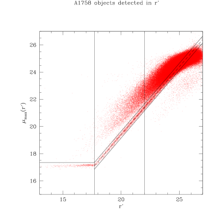
Figure 1: Central surface brightness in the $r^{\prime}$ band as a function of $r^{\prime}$ magnitude. The horizontal and oblique full lines isolate the star sequence (below the horizontal line and between the oblique lines). The two vertical lines correspond to $r^{\prime}=17.75$ where the stars stop being saturated, and $r^{\prime}=22$, where the fit to calculate the star sequence was limited (see text).

The best fit to the star sequence visible on Fig. 1 calculated for $17.75<r^{\prime}<22$ is $\mu_{max}=0.996r^{\prime}-0.524$, with standard deviations on the slope and constant of 0.002 and 0.035 respectively. The point-source (hereafter called “star”) sequence is clearly visible for $r^{\prime}<22$, with the star saturation showing well for $r^{\prime}<17.75$. We will define galaxies as the objects with $\mu_{max}(r^{\prime})>17.4$ for $r^{\prime}<17.75$, and as the objects above the line of equation $\mu_{max}=0.996r^{\prime}-0.274$ for $r^{\prime}\geq 17.75$. Stars will be defined as all the other objects (see Fig. 1). The small cloud of points observed in Fig. 1 under the star sequence is in fact defects, but represents less than 2% of the number of stars. We thus obtained a star and a galaxy catalogue.

As a check to see up to what magnitude we could trust our star-galaxy separation, we retrieved the star catalogue from the Besançon model for our Galaxy (Robin et al. 2003) in a 1 deg² region centered on the position of the image analysed here. Such a catalogue is in AB magnitudes (as ours) and is corrected for extinction. In order for it to be directly comparable to our star catalogue, we corrected our star catalogue (and our galaxy catalogue as well, for later purposes) for extinction: 0.0531 mag in $g^{\prime}$ and 0.0385 mag in $r^{\prime}$ (as derived from the Schlegel et al. 1998 maps).

The $r^{\prime}$ magnitude histogram of the objects classified as stars in our $r^{\prime}$ image roughly agrees with the Besançon star catalogue for $r^{\prime}\leq$22. However, for $r^{\prime}>$21, we start to detect more stars than predicted by the Besançon model (the difference is only about 15% at $r^{\prime}=21.5$ but becomes 25% in the $r^{\prime}=22$ bin, and the difference continues to increase at fainter magnitudes).

We will therefore consider that our star-galaxy separation is correct for $r^{\prime}\leq 22$. For fainter magnitudes, we will compute galaxy counts by counting the total number of objects (galaxies plus stars) per bin of 0.5 mag, and considering that the number of galaxies is equal to the total number of objects minus the number of stars predicted in each bin by the Besançon model.

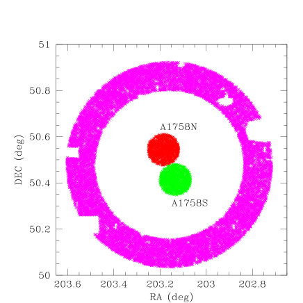
Figure 2: Positions of the objects (stars and galaxies) in the Abell 1758 North (red) and South (green) catalogues. The objects used to estimate background counts (see text) are shown in magenta. Note that the figure covers $1\times 1$ deg², and is slightly smaller than the images.

We extracted from the star and galaxy catalogues two catalogues as large as possible corresponding to the North and South clusters. Their respective positions were taken to be the X-ray centers of the two clusters, as derived from XMM-Newton data: 203.1851,+50.5445 (J2000.0, in degrees) for the North cluster, and 203.1335,+50.4138 for the South one. The maximum possible radius to obtain independent catalogues for each of the two clusters was 0.0675 deg, or 1.03 Mpc at a redshift of 0.279.

We obtained for each of the two clusters three complementary catalogues (with $g^{\prime}$ and $r^{\prime}$ magnitudes): objects classified as galaxies (classification valid at least for $r^{\prime}\leq 22$), objects classified as stars, and a complete catalogue of galaxies+stars which will be used for $r^{\prime}>22$. The positions of the galaxies in the regions of the two clusters are shown in Fig. 2.

2.3 Catalogue completeness

Figure 3: Point source completeness as a function of magnitude in percentages for Abell 1758 North (top) and South (bottom) in $g^{\prime}$ (left) and $r^{\prime}$ (right) for point–like objects (see text).

The completeness of the catalogue is estimated by simulations. For this, we add “artificial stars” (i.e. 2-dimensional Gaussian profiles with the same Full-Width at Half Maximum as the average image Point Spread Function) of different magnitudes to the CCD images and then attempt to recover them by running SExtractor again with the same parameters used for object detection and classification on the original images. In this way, the completeness is measured on the original images.

In practice, we extract from the full field of view two subimages, each $1300\times 1300$ pixels², corresponding to the positions of the two clusters on the image.

In each subfield, and for each 0.5 magnitude bin between $r^{\prime}=20$ and 27, we generate and add to the image one star that we then try to detect with SExtractor, assuming the same parameters as previously. This process is repeated 100 times for each of the two fields and bands.

Such simulations give a completeness percentage for stars. This is obviously an upper limit for the completeness level for galaxies, since stars are easier to detect than galaxies. However, we have shown in a previous paper that this method gives a good estimate of the completeness for normal galaxies if we apply a shift of $\sim 0.5$ mag (see Adami et al. 2006). Results are shown in Fig. 3.

From these simulations, and taking into account the fact that results are worse by $\sim 0.5$ mag for mean galaxy populations than for stars, we can consider that our galaxy catalogues are complete to better than 80% for $g^{\prime}\leq 25.8$ and $r^{\prime}\leq 25.6$ in both clusters.

2.4 Galaxy counts

The surfaces covered by the Abell 1758 North and South catalogues (after excluding masked regions) are 0.01412 deg² and 0.01418 deg² respectively. Galaxy counts were computed in bins of 0.5 mag normalized to a surface of 1 deg².

For $r^{\prime}\leq 22$, galaxy counts were derived directly by computing histograms of the numbers of galaxies in the Abell 1758 North and South catalogues. For $r^{\prime}>22$, we built for each cluster histograms of the total numbers of objects (galaxies+stars) and obtained galaxy counts by subtracting the numbers of stars predicted by the Besançon model. The resulting galaxy counts will be used in the next section to derive the GLFs for both clusters in both bands.

As a test, we considered the galaxy counts in the 21.5–22.0 magnitude bin computed for both clusters with the two methods (i.e. first method: considering that the star-galaxy separation is valid, and second method: considering the total number of objects (galaxies+stars) and subtracting the number of stars predicted by the Besançon model to obtain the number of galaxies). In all cases, the differences are smaller than 4%.

Note that no k-correction was applied to the galaxy magnitudes.

3 Results: colour-magnitude diagrams and galaxy luminosity functions

In order to compute the galaxy luminosity functions of the two clusters, we need to subtract to the total galaxy counts the number counts corresponding to the contamination by the foreground and background galaxies.

For galaxies brighter than $r^{\prime}=22$ we will select galaxies with a high probability to belong to the clusters by drawing colour-magnitude diagrams and selecting galaxies located close to this relation. A few spirals may be missed in this way, but their number in any case is expected to be small, as explained in Sect. 3.1 (also see e.g. Adami et al. 1998). For galaxies fainter than $r\prime=22$ we will subtract galaxy counts statistically.

3.1 Colour–magnitude diagram

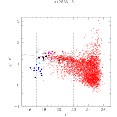
Figure 4: $(g\prime-r\prime)$ vs. $r^{\prime}$ colour–magnitude diagram for Abell 1758 (North and South) for objects classified as galaxies from the $\mu_{max}-r\prime$ magnitude relation. The vertical dashed lines indicate the magnitude interval where the colour-magnitude relation was computed. The long oblique dashed line shows the mean colour-magnitude relation; the short oblique dotted lines indicate intervals of $\pm 1\sigma,2\sigma$ and $3\sigma$ around the colour-magnitude relation. The interval finally adopted of $1.5\sigma$ is shown with full lines. The filled circles show the galaxies with measured redshifts, colour–coded as follows: black: galaxies belonging to the cluster according to their spectroscopic redshifts, cyan and magenta for galaxies with smaller and larger redshifts than the cluster, but inside the two circles where the two clusters were extracted, blue and red: galaxies with smaller and larger redshifts than the cluster, but outside these two circles.

The $g^{\prime}-r^{\prime}$ vs. $r^{\prime}$ colour–magnitude diagram is shown in Fig. 4 for the two clusters together (the diagrams are the same for both clusters). A sequence is well defined for galaxies in the magnitude range $17<r^{\prime}<22$ in both clusters. We computed the best fit to the $g^{\prime}-r^{\prime}$ vs. $r^{\prime}$ relations in this magnitude range by applying a linear regression. We then eliminated the galaxies located more than 3$\sigma$ away from this relation and computed the $g^{\prime}-r^{\prime}$ vs. $r^{\prime}$ relation again.

The equation of the colour–magnitude relation is found to be: $g^{\prime}-r^{\prime}=-0.0436r^{\prime}+2.108$ with an r.m.s. on the constant $\sigma=0.11$.

We also plot in Fig. 4 galaxies with measured spectroscopic redshifts. We can see that the positions of the galaxies belonging to the cluster according to their spectroscopic redshifts, i.e. with redshifts in the [0.264, 0.294] interval fall very close to the best fit to the colour–magnitude relation.

In view of this, for $r^{\prime}\leq 22$, we will consider hereafter that all the galaxies located within $\pm 1.5\sigma$ of the colour–magnitude relation (i.e. between the two black lines of Fig. 4) belong to the cluster.

We can note that the scatter $\sigma=0.11$ is somewhat larger than found in the Abell 222/223 clusters at z=0.21 (Durret et al. 2010), but the interval chosen for cluster membership ($\pm 1.5\sigma$) remains smaller than that used for example by Laganá et al. (2010) in the redshift interval [0.11,0.23].

The initial sample of galaxies comprises 1599 and 1438 galaxies in the North and South clusters respectively (with no magnitude limit). Within the $\pm 1.5\sigma$ interval along the red sequence, we are left with respective numbers of galaxies of 477 and 340. These numbers become 192 and 116 galaxies for $r^{\prime}\leq 22$. The North cluster is obviously richer than the South one.

With this rather strict criterium, we obviously select galaxies with a high probability to belong to the cluster, but we may lose some galaxies, in particular blue cluster galaxies falling under the sequence.

We have therefore estimated the number of blue cluster galaxies lost by selecting galaxies within $\pm 1.5\sigma$ of the red sequence in the following way. First, we computed histograms of numbers of galaxies within $\pm 1.5\sigma$ of the red sequence and below this sequence in bins of 1 absolute magnitude in the $r^{\prime}$ band. These counts were made in absolute magnitude bins to be comparable to the counts estimated from luminosity functions of field galaxies. The bins of interest here are between ${\rm M_{r^{\prime}}=-22}$ and $-19$, roughly corresponding to $r^{\prime}=18.5$ and 21.5. We then computed the number of foreground galaxies expected. Since the comoving volume at z=0.279 is 5.834 Gpc³ (Wright 2006), and each of our clusters covers an area of 0.01431 deg² on the sky, the volume in the direction of each cluster is 2024 Mpc³. By using the R band luminosity function by Ilbert et al. (2005) in the 0.05-0.20 redshift bin (see their Fig. 6 and Table 1), we find that the percentages of “lost” galaxies are of the order of 30% for ${\rm M}_{r^{\prime}}=-19$, of 10%–15% for ${\rm M}_{r^{\prime}}=-20$ and $-21$, and less than 10% for brighter galaxies.

3.2 Comparison field

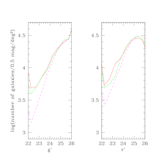
Figure 5: Galaxy counts in the $g^{\prime}$ (left) and $r^{\prime}$ (right) bands for magnitudes $r^{\prime}>22$ where the background must be subtracted statistically, in logarithmic scale. The counts in Abell 1758 North and South are drawn in red and green respectively. The magenta dashed lines show the galaxy counts from the “local” background extracted in the annulus shown in Fig. 2. Error bars are Poissonian and are not plotted for clarity.

In order to perform a statistical subtraction of the background contribution for $r^{\prime}>22$, and since the cluster is quite distant and does not cover the whole field, we extracted background counts in an annulus surrounding the clusters (see Fig. 2). The annulus was centered on the middle position between the two clusters (203.1593,+50.4792 J2000.0 in degrees), with an inner radius of 0.3232 deg (4.9 Mpc), and an outer radius of 0.4444 deg (6.8 Mpc). The unmasked surface of the annulus is 0.278 deg².

We checked if there could be any contamination of background counts in this annulus by a group or cluster, and found a structure west-southwest of Abell 1758. This appears as a cluster in Simbad with coordinates 13^h34^mn45.41^s, +50^∘26’01.4” (J2000.0) and redshift 0.085. The mean redshift for the 20 galaxies extracted from NED (http://nedwww.ipac.caltech.edu/) in this region is 0.0869, with a dispersion in redshift $\sigma_{z}=0.0015$. This cluster falls just outside the annulus which was used to estimate the background counts subtracted to the galaxy counts to compute the GLF, so its presence should not modify galaxy counts inside the annulus.

We can note from Fig. 5 that galaxy counts are comparable in Abell 1758 North and South in the $g^{\prime}$ band, but differ in the $r^{\prime}$ band, where Abell 1758 North has more galaxies in the $22\leq r^{\prime}\leq 24$ magnitude range.

3.3 Galaxy luminosity functions

The Galaxy Luminosity Functions (GLFs) of Abell 1758 North and South were calculated in bins of 0.5 mag and normalized to 1 deg². We subtracted the background contribution using as background galaxy counts the “local” counts in the annulus shown in magenta in Fig. 2.

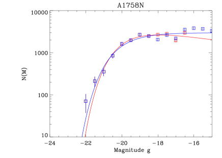
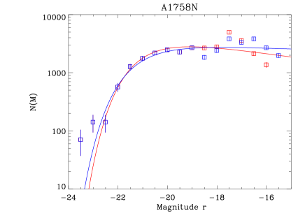
Figure 6: Galaxy luminosity functions for Abell 1758 North in the $g^{\prime}$ (top) and $r^{\prime}$ (bottom) bands, in logarithmic scale. The blue and red points correspond to the two galaxy selections (see text), and the best Schechter function fits are drawn with the same colours as the corresponding points. Note that at bright magnitudes, the points exactly coincide, and since the blue points were plotted after the red ones, they appear blue. Error bars are 4 times the Poissonian errors on galaxy counts (see text).

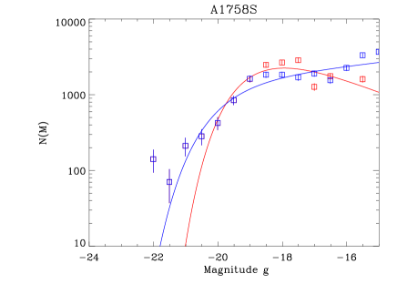
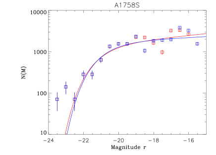
Figure 7: Same as Fig. 6 for the South cluster.

The GLFs are displayed for Abell 1758 North and South in Figs. 6 and 7 respectively (red points). The error bars drawn in these figures were taken to be 4 times the Poissonian errors on galaxy counts, as derived from detailed simulations previously performed by our team for similar data (see Boué et al. 2008,  Fig. 5).

The GLFs (as a function of absolute magnitude) were fit by a Schechter function:

$$S(M)=0.4\,\ln 10\,\phi^{\ast}\,y^{\alpha+1}\,e^{-y}$$

with $y=10^{0.4\,(M^{\ast}-M)}$.

The parameters of the Schechter function fits of the GLFs are given in Table 2. The absolute magnitude ranges considered are indicated for each fit, and GLFs and their fits are drawn in Figs. 6 and 7.

Table 2: Schechter parameters for galaxy luminosity functions. The first set of fits corresponds to galaxies selected from the colour-magnitude relation for $r^{\prime}<22$ and to a statistical background subtraction with galaxy counts taken from the CFHTLS Deep field counts for $r^{\prime}>22$. The second set of fits corresponds to galaxies selected from the colour-magnitude relation at all magnitudes. The last line corresponds to the fit to the simulated GLF (see text).

Cluster	Filter	Range	$\Phi^{*}$	M∗	$\alpha$
North	$g^{\prime}$	$-22.0,-16.5$	$4384\pm 462$	$-20.06\pm 0.12$	$-0.86\pm 0.05$
	$r^{\prime}$	$-23.5,-16.0$	$4650\pm 286$	$-21.18\pm 0.08$	$-0.85\pm 0.02$
South	$g^{\prime}$	$-22.0,-15.5$	$5319\pm 574$	$-18.90\pm 0.14$	$-0.59\pm 0.08$
	$r^{\prime}$	$-23.5,-16.0$	$1582\pm 229$	$-21.34\pm 0.16$	$-1.11\pm 0.04$
North	$g^{\prime}$	$[-22.0,-16.5]$	$3244\pm 236$	$-20.33\pm 0.09$	$-1.00\pm 0.02$
	$r^{\prime}$	$[-23.5,-16.0]$	$3451\pm 229$	$-21.44\pm 0.08$	$-0.96\pm 0.02$
South	$g^{\prime}$	$[-22.0,-15.5]$	$1652\pm 205$	$-20.09\pm 0.16$	$-1.12\pm 0.03$
	$r^{\prime}$	$[-23.5,-16.0]$	$1849\pm 195$	$-21.18\pm 0.14$	$-1.06\pm 0.03$
Simulated		$[-25.0,-15.0]$	$755\pm 21$	$-22.09\pm 0.04$	$-1.01\pm 0.01$

If we look at Abell 1758 North (Fig. 6) we see that a Schechter function fits rather well most of the GLF points for both bands. However, there is an excess of galaxies over a Schechter function in the very brightest magnitude bins, specially in the $r^{\prime}$ band. There is also a “bump” around $r^{\prime}$ absolute magnitudes $-17$ and $-17.5$ which has no obvious explanation. Except for this feature, the GLFs are quite similar in both bands, and the faint end slopes are quite flat: $\alpha=-0.85$.

On the other hand, for Abell 1758 South (Fig. 7), the GLFs are not well fit by Schechter functions. In the $g^{\prime}$ band, there is a strong excess of galaxies at bright magnitudes, and the faint end slope is quite flat ($\alpha=-0.59$), implying that star formation is weak in faint galaxies of the South cluster. In the $r^{\prime}$ band, the GLF also shows an excess at very bright magnitudes, and a strong dip for ${\rm M_{r^{\prime}}\sim-17.5}$. This dip is also seen in the $g^{\prime}$ band around $-17$, though it is not as pronounced as in the $r^{\prime}$ band. Note that in the South cluster the GLFs in the $g^{\prime}$ and $r^{\prime}$ bands have quite different faint end slopes: $\alpha=-0.59$ in $g^{\prime}$ and $\alpha=-1.11$ in $r^{\prime}$. This lack of blue faint galaxies could suggest that star formation has been quenched by a process linked to the merger, but could also be an artefact due to the method used here to derive the GLF (see end of Sect. 3.4).

The fact that both clusters have GLFs differing from simple Schechter functions is most probably due to the fact that both are undergoing merging processes, as already pointed out by David & Kempner (2004) from their X-ray study. We will discuss these results in the next Section when considering the temperature and metallicity distributions of the X-ray gas. These maps confirm that both clusters are indeed structures which are strongly pertubed by several mergers, so it is not surprising to see effects on the GLFs.

Altogether, the GLFs in Abell 1758 do not strongly differ from those derived in other clusters. The bright parts of the GLF Schechter fits (${\rm M_{r^{\prime}}<-19}$) for both clusters are quite similar in shape to the GLFs recently obtained by other authors (see for example Andreon et al. 2008). And the faint end slopes are within the broad range of values estimated by previous authors for different clusters, cluster regions and photometric bands (see e.g. the compilation in Table A1 of Boué et al. 2008), except for the South cluster in the $g^{\prime}$ band, where the GLF seems unusually flat.

Note that Abell 1758 is at redshift 0.279, and few GLFs are available for clusters at such redshifts. Andreon et al. (2005) found more or less comparable faint end slopes of $-1.03$ and $-1.30$ for two clusters at redshifts $\sim 0.3$, but in the K band, so the comparison with our results is not straightforward.

3.4 Galaxy luminosity functions only based on a colour-magnitude selection

As a test to our method, we also derived the GLFs by considering that all the galaxies located within $\pm 1.5\sigma$ of the colour-magnitude relation shown in Fig. 4 were cluster members, for all magnitudes.

The corresponding points and GLF Schechter fits are shown in blue in Figs. 6 and 7 and the corresponding Schechter parameters are given in the second half of Table 2. We can see that for absolute magnitudes fainter than about $-19$ to $-18$ the data points of the GLFs start to differ. The agreement between the Schechter fits based on the two methods is fair for the North cluster in both bands and for the South cluster in the $r^{\prime}$ band, though the Schechter parameters found in corresponding cases are not always within error bars. This strongly suggests that the errors on these parameters are underestimated, and this is probably also the case for the errors on the GLF points themselves. On the other hand, the agreement is poor for the South cluster in the $g^{\prime}$ band. Therefore we cannot consider that the $g^{\prime}$ band GLF is well constrained in the South cluster.

These results clearly illustrate the difficulty to estimate GLFs, particularly at faint magnitudes, as already mentioned by a number of authors (see discussion in Durret et al. 2010). They also justify our choice not to attempt GLF fits with a higher number of free parameters, as would be obtained by fitting a gaussian at bright magnitudes plus a Schechter function at faint magnitudes, or two Schechter functions.

3.5 Simulated galaxy luminosity function

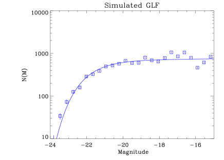
Figure 8: Simulated luminosity function with best Schechter fit superimposed.

In connection with the numerical simulations presented in Section 5, we simulated a galaxy luminosity function using the halo mass–luminosity relation from Vale & Ostriker (2006). The halo mass for the simulated galaxies is taken from the galaxy formation model, which calculates the halo mass from the N-body simulation. All the simulated galaxies were put into 25 magnitude bins between absolute magnitudes $-25$ and $-15$.

The resulting GLF is shown in Fig. 8. We can see that it appears quite similar in shape to those shown in Figs. 6 and 7. A Schechter fit to this function is superimposed in Fig. 8 and its parameters are given in Table 2. We can see that although the value of $M^{*}$ is between half a magnitude and a magnitude brighter, the faint-end slope agrees well with the values derived from the observations.

3.6 Do the North and South clusters have a cD galaxy?

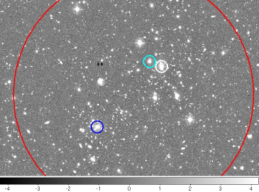
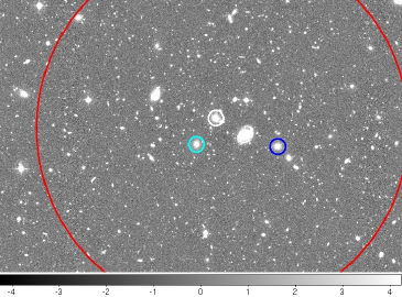
Figure 9: Optical images of Abell 1758 North (top) and South (bottom). For each cluster, the brightest galaxy is circled in black, the second brightest in blue and the third brightest in cyan. The red circles show the cluster limits. The uncircled galaxy near the center of the South cluster is a foreground object.

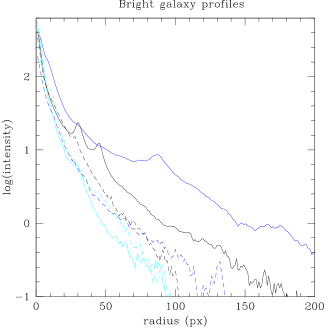
Figure 10: Surface brightness profiles of the three brightest galaxies in both clusters (intensities are normalized to the central value and in arbitrary units, and radii are in pixels). Full and dashed lines correspond to galaxies in the North and South clusters respectively. For each cluster, the brightest galaxy is in black, the second brightest in blue and the third brightest in cyan.

The images of the three brightest galaxies of each cluster are shown in Fig. 9. We can see that in the North cluster none of these galaxies is at the cluster centre, and there are obviously two subclusters. In the South cluster, none of the three brightest galaxies is perfectly in the centre either (the galaxy which is not circled is a foreground object).

The similarity with the Abell 222/223 cluster pair (see Durret et al. 2010,  figure 20) has led us to analyze the brightness profiles of the brightest galaxies in the Abell 1758 North and South clusters. We had found that Abell 223 (which resembles Abell 1758 North) had two Brightest Cluster Galaxies (BCGs), one of them showing a brightness profile decreasing slowlier than the other, and therefore resembling that of a cD, while the other one could be the central galaxy of an accreted group.

The surface brightness profiles of the three brightest galaxies in the two Abell 1758 clusters are displayed in Fig. 10. We can see that the profiles of the two brightest galaxies of the North cluster decrease notably slowlier with radius that those of the other bright galaxies, and surprisingly, the profile of the second brightest galaxy is much flatter than that of the brightest one. This suggests that there are two dominant galaxies in the North cluster, quite similarly to what was seen in Abell 223, and this is another indication of a merger. The fact of having two dominant galaxies is probably another indication of a merger of two smaller systems, in agreement with David & Kempner (2004) who suggested that at least two smaller clusters have crossed this North system. On the other hand, there is no dominant galaxy in the South cluster, where the profiles of the three brightest galaxies are comparable.

4 X-ray analysis

We present in Fig. 11 the X-ray surface brightness isocontours oveplotted on the optical $r^{\prime}$ band image of Abell 1758 and indicate the positions of the three brightest galaxies of each cluster. The three galaxies of each cluster are the remaining central galaxies from the ancient sub-clusters. Another important thing to notice is their position: the two brightest galaxies one near the other and the third one is radially opposite. This is an indication of a recent merger where we clearly see that while the gas has already settled down, the brightest galaxies are not in the center of Abell 1758 North and A1758 South. We will revisit this merging scenario in the following sections.

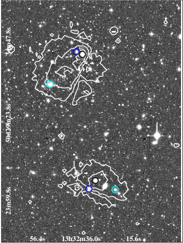
Figure 11: Optical image with X-ray isocontours superimposed. The circles correspond to the three brightest galaxies in Abell 1758 North. The colors are the same as in Fig. 10: the brightest galaxy is in black, the second brightest in blue and the third brightest in cyan.

4.1 Data reduction

Abell 1758 was observed for $\sim$57 ks with XMM-Newton with the Medium filter inserted. The XMM-Newton ODF files were processed using SAS version v8.0. The MOS and pn files were filtered excluding all events with FLAG $>$ 0 and PATTERN $>$ 12, and FLAG $>$ 0 and PATTERN $>$ 4, respectively. Light curves were made in the 1–10 keV energy band and periods where the background value exceeded the mean value by more than 3$\sigma$ were excluded. We considered events inside the field of view (FOV) and excluded all bad pixels. Flare filtering left live times of 16928 s, 12734 s and 16929 s in the MOS1, MOS2 and pn cameras respectively.

The background was taken into account by extracting MOS1, MOS2 and pn spectra from the publicly available EPIC blank sky templates of Andy Read (Read & Ponman 2003). The background was normalized using a spectrum obtained in an annulus (between 12.5–14 arcmin) where the cluster emission is no longer detected.

4.2 Spectrally measured 2D X-ray maps

We performed quantitative studies using X-ray spectrally measured 2D maps to derive global properties of these two clusters. These maps were made in a grid; for each spatial bin we set a minimum count number of 900 (after background subtraction). For the spectral fits, we used XSPEC version 11.0.1 (Arnaud 1996) and modeled the obtained spectra with a MEKAL single temperature plasma emission model (bremsstrahlung + line emission Kaastra & Mewe 1993; Liedahl et al. 1995). The free parameters are the X-ray temperature (kT) and the metal abundance (metallicity). Spectral fits were made in the energy interval of 0.7$-$8.0 keV with the hydrogen column density fixed at the Galactic value ($1.06\times 10^{20}\leavevmode\nobreak\ \rm cm^{-2}$), estimated with the nH task of FTOOLS (based on Dickey & Lockman 1990).

We compute the effective area files (ARFs) and the response matrices (RMFs) for each region in the grid. This procedure (already described in Durret et al. 2010) allows us to perform a reliable spectral analysis in each spatial bin, in order to derive high precision temperature and metallicity maps, since we simultaneously fit all three instruments. The best fit value is then attributed to the central pixel.

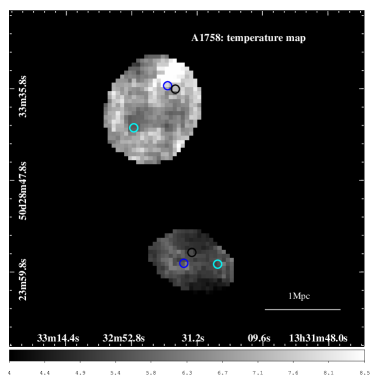
Figure 12: X-ray temperature map for Abell 1758 North (top) and South (bottom). The color-bar indicates the temperature in keV. The circles correspond to the three brightest galaxies in each cluster. The colors are the same as in Fig. 10: the brightest galaxy is in black, the second brightest in blue and the third brightest in cyan. The corresponding error map is shown in Fig. 15 (top).

ht!

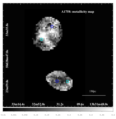
Figure 13: X-ray metallicity map for Abell 1758 North (top) and South (bottom). The color-bar indicates the metallicity in solar units. The circles correspond to the three brightest galaxies in each cluster. The colors are the same as in Fig. 10: the brightest galaxy is in black, the second brightest in blue and the third brightest in cyan. The corresponding error map is shown in Fig. 15 (bottom).

The resulting X-ray temperature and metallicity maps are displayed in Figs. 12 and 13. Maps of the errors on these two maps are given in the Appendix (Fig. 15).

The temperature maps in Fig. 12 show that both clusters appear almost isothermal, the North one being hotter ($\sim 6-7$ keV) and the South one being cooler ($\sim 4-5$ keV). The presence of inhomogeneities is not obvious in the temperature maps, except for a hotter blob in the northwest region of Abell 1758 North. Although signs of recent interactions are not clearly present in the temperature map, the positions of the three brightest galaxies argue in favour of a merging scenario where two clusters merged to form Abell 1758 North, as mentioned in Sect. 4.

On the other hand, two striking aspects call the attention when considering the metallicity map shown in Fig. 13. First, we can note two elongated regions of high metallicity in the North cluster, suggesting that at least two smaller clusters have crossed the North cluster (as pointed out by David & Kempner 2004). Based on the positions of the three brightest galaxies we can assume a scenario in which these elongated regions are due to metals were ton by ram-pressure stripping during the merger.

Second, the metallicity map of the South cluster is even more unusual, since it shows a deficit of metals in the central region. This deficit is probably the signature of an interaction with the central object. Since this cluster is less massive, the effects of galactic winds or supernova explosions will be stronger to expell metals towards the outskirts (Evrard et al. 2008).

However, none of the metal structures identified in the 2D maps correlates with any temperature structure for either cluster. We do not see the high-metallicity regions of the North cluster in the temperature map.

To have an overview of the merging scenario and better understand the dynamical history of these clusters, we considered the results of numerical simulations to give support to our findings, and compared them with our observational results. This will be presented in the next section.

David & Kempner (2004) have already analyzed this system using XMM-Newton and Chandra data. They conclude that these two clusters most likely form a gravitationally bound system, though their imaging and spectroscopic analyses do not reveal any sign of interaction between the North and South clusters, and show that A1758N and A1758S are both undergoing major mergers. It is clear from our analysis that Abell 1758 North is still undergoing at least one merger, the bright and hot zone seen in the temperature map probably being the signature of one of the cores. For Abell 1758 South, the merger is not evident in X-rays, though some kind of interaction is suggested by the absence of a cool core, and confirmed by the optical data analysis.

5 Numerical simulation results

As described in detail in Kapferer et al. (2006) Kapferer et al. (2007) or Schindler et al. (2005) we combine several codes to model the metal distribution in a galaxy cluster. To calculate the dark matter structure of the galaxy cluster we use the N-body code GADGET2 (Springel 2005) with constrained random fields as initial conditions (Hoffman & Ribak 1991).A semi-analytical galaxy-formation model then assigns galaxy properties to the halos found in the dark matter structure. For this galaxy-formation model we use an improved version of the code described by van Kampen et al. (1999). The chemical evolution of the galaxies is modeled as in Matteucci & François (1989). To study the evolution of the ICM we use a hydrodynamic grid code with comoving coordinates and a PPM-scheme for a better treatment of shocks (Colella 1984). To optimize the computational time, we use 4 nested grids (Ruffert 1992), each with 128x128x128 cells. The total computational hydro-volume has a side length of 20 Mpc. We included special routines to transport enriched material out from the modelled galaxies into the ICM: we model ram-pressure stripping as well as galactic winds as described in Gunn & Gott (1972); Domainko & Kapferer (2006); Kapferer et al. (2007). More specifically, the ram-pressure and galactic wind algorithms calculate a mass loss for each model galaxy (depending on its velocity relative to the ICM and its star formation rate). As the galaxy formation model provides us with the metallicity within the ISM, we know the quantity of metals transported from the ISM into the ICM. These metals are then advected with the ICM, and by knowing the ICM density we can then calculate the ICM metallicity. Combining these codes, we can simulate the 3D evolution of the ICM and its metallicity. From these 3D data, we then extract temperature and metal maps, by making emission weighted projections. These maps can be compared directly to observations.

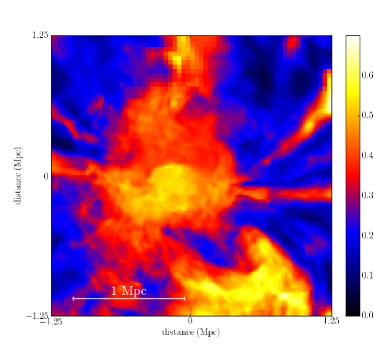
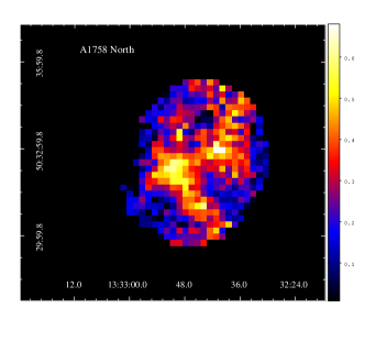
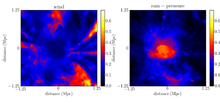
Figure 14: Top left panel: metal distribution predicted by numerical simulations at the cluster redshift (i.e. sum of the two panels below). Top right panel: observed metal distribution map in Abell 1758 North. Both panels have a side-length of 2.5 Mpc. Bottom left panel: metals which were ejected by galactic winds. Bottom right panel: metals which were transported out of the galaxies by ram-pressure stripping.

We performed 5 simulations with different initial conditions and selected the simulation which best matched our observational results. It should be noted that we did not set up the simulations to specifically reproduce Abell 1758. Among all the tests perfomed here, we found one metal distribution that reproduces quite reasonably the elongated region of high abundance found observationally for the North cluster. We see that the simulated 2D map in Fig. 14 can also reproduce the exact values for the metallicity of the North cluster. For the bright regions (in yellow color) we have metallicity values of about $0.5-0.6$ solar units. The metallicity decreases towards the outskirts where it reaches values around 0.2 solar units.

It is of great importance to mention the spatial scales of the features presented in the 2D metal distribution maps predicted by numerical simulations and derived from observations. The physical sizes of the two top panels in Fig. 14 are exactly the same (a side-length of 2.5 Mpc), but the features, although similar in shape, do not have the same physical sizes. In the observational metal distribution (top right panel in Fig. 14) we see that Abell 1758 North is completely comprised within 2.5 Mpc, while in the metal distribution computed from numerical simulations (top left panel in Fig. 14) the cluster extends over a larger region. The point here is that we did not make the simulations to exactly match this cluster.

In order to analyze the importance of galactic winds and ram-pressure stripping in transporting metals, we display in Fig. 14 the results of numerical simulations, showing separately the metals ejected by galactic winds (bottom left), those transported out of the galaxies by ram-pressure stripping (bottom right), and the sum of the metals accounted for by these two processes (top left). These maps can be compared to the metallicity map derived from observations for the North cluster (top right). From these figures, we can say that both processes are important for metal enrichment, playing different roles in the cluster, with winds definitely playing a higher part in the south-west corner. Galactic winds are more important in the outskirts of the cluster, while ram-pressure stripping seems to be dominant in the inner parts.

It is worth noting the time scales of these different enrichment processes. By analyzing the results of our numerical simulation, we can say that a large part of the metals for the high metallicity region in the south of Abell 1758 North and the thin elongated stripe from the center to the north-west have been transported into the ICM at redshifts z$>3$. Then, between redshifts 3 and 2 there was a substantial contribution to the metallicity in the elongated structure but no contribution to the center of the cluster. Between redshifts 2 and 1, there was a substantial contribution to the central region (around 1/3 of the final metallicity), mainly due to ram-pressure. Then, between redshifts 1 and 0.8 there was hardly any contribution to the metallicity at all. From z=0.8 to z=0.5 there was a contribution (around 0.2 solar metallicities) to the metals in the central region, coming only from ram-pressure stripping. And finally, from z=0.5 to z=0.279 (the cluster redshift) there was hardly any significant contribution to the metallicity. In summary, many of the metals which are responsible for the features in the outskirts have been transported into the ICM at very early times, even before z=3. If we look at the metals which have been transported into the ICM before z=2, we see that they explain the main morphological features in the outskirts (like the elongated structure). On the other hand, the enrichment of the central region takes place mainly between z=2 and z=0.5, predominantly via ram-pressure stripping.

The results presented above show that the comparison of observations with the results of numerical simulations is a powerful tool to understand better the physical processes involved in the transport of metals. However, there is still work to be done on this topic, based on a larger sample of clusters in different dynamical states.

6 Discussion and Conclusions

It is becoming clear that clusters are in a continual state of evolution and with high precision telescopes, such as XMM-Newton and Chandra, we see that they are hardly ever relaxed and virialized as it was previously assumed. We have thus become interested in multiple mergers, where merging effects are expected to be even stronger.

As a second study of cluster pairs, we chose to analyse Abell 1758 (at a redshift of 0.279) by coupling archive optical CFHT Megacam and XMM-Newton data, and by comparing the temperature and metallicy maps obtained for the ICM with the results of numerical simulations. We made a step further by also considering the results of numerical simulations to try to understand better the dynamics and building-up history of this system.

From our results, signs of merger(s) are detected in the optical as well as X-ray wavelength ranges, meaning that both galaxies and gas are still out of equilibrium. From optical results we see that for Abell 1758 North, a Schechter function fits rather well most of the points of the GLFs in the $g^{\prime}$ band, but there is an excess of galaxies over a Schechter function in the brightest magnitude bins, specially in the $r^{\prime}$ band, as well as a possible and unexplained excess of galaxies around M${}_{r^{\prime}}\sim-17.5$. On the other hand, for Abell 1758 South, which is poorer than the North cluster, the GLF is not as well defined and fit by a Schechter function. Note in particular that the GLFs derived by the two methods (statistical background subtraction for $r^{\prime}>22$ or colour-magnitude selection at all magnitudes)) look quite different, particularly in the $g^{\prime}$ band. If the dip detected in the $r^{\prime}$ band GLF for M${{}_{r^{\prime}}\sim-18}$ is real, as already found in other clusters but at somewhat brighter absolute magnitudes, it could be interpreted as showing the transition zone between (brighter) ellipticals and (fainter) dwarfs (Durret et al. 1999). An excess of galaxies over a Schechter function in the brightest magnitude bins is observed in both bands. We can also note that in the South cluster the GLFs in the $g^{\prime}$ and $r^{\prime}$ bands look quite different, with a faint end slope somewhat steeper in $r^{\prime}$ than in $g^{\prime}$. The shallower faint end slope in $g^{\prime}$, if real, could be explained either by quenching of star formation due to the merger (which strips galaxies from their gas and reduces star formation), or by the fact that star formation has not yet had time to be triggered by the merger (see e.g. Bekki 1999). The somewhat perturbed shapes of the GLFs of both clusters therefore agree with the fact that they are both undergoing merging processes.

From the X-ray analysis we have noticed that the gas temperature maps do not present prominent inhomogeneities, except for a hotter blob in the northwest of Abell 1758 North. The North cluster is hotter (with temperatures in the range of $\sim 6-7$ keV) and the South one cooler (with kT $\sim 4-5$ keV). The hotter blob in the northwest of Abell 1758 North could be explained by heating of the gas in that region by the movement of the northwest system towards the north proposed by David & Kempner (2004). The most striking features are seen in the metallicity maps. The metallicity map of the South cluster is even more unusual, since it shows a deficit of metals in the central region. This deficit is probably the signature of an interaction with the central object that could have expelled metals towards the outskirts (see Evrard et al. 2008, and top left panel of Fig. 14). We also detect two elongated regions of high metallicity in the North cluster, suggesting that at least two smaller clusters have crossed the North cluster. Note that our temperature and metallicity maps are in agreement with the scenarios proposed by David & Kempner (2004), who derived that the North cluster is in the later stages of a large impact parameter merger between two 7 keV clusters, while the south cluster is in the earlier stages of a nearly head–on merger between two 5 keV clusters.

In order to understand better the nature of the most prominent features exhibited in the metallicity map of the North cluster, we performed 5 simulations with different initial conditions. It should be stressed that we did not set up the simulations to specifically reproduce Abell 1758. Among these 5 simulations, we found one metal distribution that reproduces quite reasonably the elongated region of high abundance found observationally for the North cluster, although without a perfect spatial correlation. The results of our numerical simulations allowed us to distinguish the role of metal transportation processes such as galactic winds and ram-pressure stripping. We have shown that these phenomena act in different regions of the cluster, and that in the metal-rich elongated regions of the North cluster, winds were more efficient in transporting enhanced gas to the outskirts than ram pressure stripping. These simulations also allowed us to compute the GLF, and the result is consistent with the observed GLFs.

In the hope of finding some kind of large scale structure and/or filaments linking Abell 1758 with its surroundings, we searched the NED database for galaxies with redshifts available in a region of 36 arcmin around Abell 1758 (corresponding to 9.1 Mpc at the cluster distance). We found 137 galaxies, out of which only 15 have redshifts in the approximate cluster redshift range: 0.264, 0.294 . No structure is found in the blueshifted and redshifted galaxies, except for what appears to be a cluster west of Abell 1758 (see Section 3.2). Therefore we cannot derive any argument from the large scale distribution of galaxies around Abell 1758.

To conclude, the Abell 1758 North and South clusters most likely form a gravitationally bound system, but our imaging analyses of the X-ray and optical data do not reveal any sign of interaction between the two clusters. All signs of dynamical disturbance are associated with recent merger(s) which each of the two clusters is still undergoing.

Appendix A Error maps

In Fig. 15 we present the errors associated to each bin in the temperature and metallicity maps displayed in Figs. 12 and 13. The errors on these parameters were directly obtained from the spectral fits.

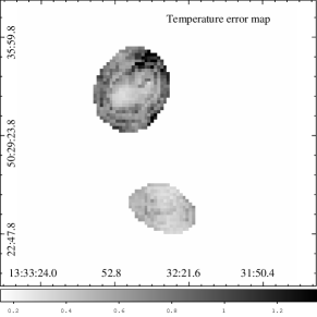
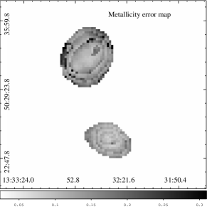
Figure 15: Upper panel: error map on the X-ray temperature. Lower panel: error map on the X-ray metallicity.

Looking at Figs. 12, 13 and 15 (error maps) we see that, for the temperature estimates, we have errors around 5% for A1758 South, while for A1758 North they vary from 5% (in the inner parts) up to 12% (at the outskirts). The errors on the temperature maps are therefore very reasonable. For the metallicity maps we do not have the same accuracy. Looking at the same figures, we see that for A1758 South, the metallicity errors can reach 25% and for A1758 North they vary from 30% (in the inner region) up to 46% (at the outskirts). It is important to notice that although the XMM-Newton exposure time on Abell 1758 was about 57 ks, due to flare filtering only $\approx$ 17 ks of good data were useable to construct the 2D spectral maps.