Finding the Rikitake’s attractors by parameter switching

Abstract

In this paper the attractors synthesis algorithm for a class of dissipative dynamical systems with hyperbolic equilibria, presented in [1], is applied to generate any attractor of the Rikitake system. By switching periodically, or even randomly, the control parameter inside a given set of values, during any finite time interval while the attractor is numerically approximated, any attractor can be generated. Beside the extension of the synthesis algorithm to systems with non-hyperbolic equilibria, we have found for the Rikitake system, a new intriguing transient which, occurring for a long time interval, is difficult to be numerically found due to the known system instability along the $x_{3}$-axis.

Keywords: Rikitake dynamo, parameter switching, attractor, attractor synthesis

1 Introduction

The paleomagnetic records of the Earth’s magnetic field show that the field has changed its polarity many times along geological history (hundreds of times during the last 160 million years). But intervals among such geomagnetic polarity reversals are highly irregular. Thus while their average is about $7.10^{5}$ years, there are intervals as long as $3.10^{7}$ years without polarity change, but with large deviations of the poles from actual positions.

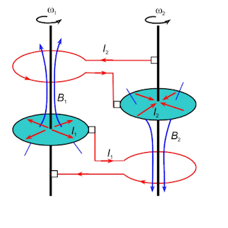
There are many factors which can affect the Earth’s magnetic field. For example the Reynolds number of the Earth’s liquid core is believed to be of the order of $10^{8}$, i.e. sufficiently large that the flow of electrical currents in the liquid core be turbulent. Hence the pattern of the Earth’s magnetic field is very complex (see for ex.[2, 3]). Because of such great complexity, to study the reversals of the Earth’s magnetic field, relatively simple mechanical dynamos had been proposed as analog models [4, 5, 6]. One of them is the Rikitake dynamo of two frictionless coupled disks, which is a paradigm of the geomagnetic field behavior, proposed by the Japanese geophysicist Rikitake [4]. This model can be considered only as a special case for the real geodynamo, which is obviously a high order physical system with very large degrees of freedom [7, 8]. The Rikitake dynamo is composed of two conducting rotating disks which are connected to two coils so that the current in each coil feeds the magnetic field of the other (see Fig.1). Each circuit has the same self-inductance $L$ and electrical resistance $R$, and for each disk dynamo a constant mechanical torque $G$ is applied from outside on the axis, so that it can rotate with the angular velocity $\omega.$

The currents $I_{1}$ and $I_{2}$ in the circuits and the related voltages $V_{1}$ and $V_{2}$ are connected by the well known relations for the $R,~{}L$ circuits

$$\begin{array}[c]{c}RI_{1}+L\frac{dI_{1}}{dt}=MI_{1}\omega_{1},\\ RI_{2}+L\frac{dI_{2}}{dt}=MI_{2}\omega_{2},\end{array}$$

where $MI_{1}\omega_{1}$ and $MI_{2}\omega_{2}~{}$are the voltages $V_{1}$ and $V_{2}$ , and $M$ is the mutual inductance. If $C$ is considered the moment of inertia of each disk, these relations can be rescaled and lead finally (see for ex [9]) to the model equations

$$\begin{array}[c]{cl}\overset{.}{x}_{1}=&x_{2}\ast x_{3}-ax_{1},\\ \overset{.}{x}_{2}=&(x_{3}-p)x_{1}-ax_{2},\\ \overset{.}{x}_{3}=&1-x_{1}x_{2},\end{array}$$ (1)

with $a=R\sqrt{\frac{LC}{GM}}$, and $\ p=\left(\omega_{1}-\omega_{2}\right)\sqrt{\frac{CM}{GL}}$. The control parameter $p$ is considered to be positive.

The system is invariant under the change $\left(x_{1},x_{2},x_{3}\right)\longmapsto\left(-x_{1},-x_{2},x_{3}\right)$. Therefore if $\left(x_{1}(t),x_{2}(t),x_{3}(t)\right)$ is a solution to (1), then $\left(-x_{1}(t),-x_{2}(t),x_{3}(t)\right)$ is also a solution.

The system is dissipative the divergence being negative $divf(x)=-2p,~{}$where the vector function $f:\mathbb{R}^{3}\rightarrow\mathbb{R}^{3}$ is the right hand side of (1).

The equilibrium points are

$$X_{1,2}\left(\pm k,\pm\frac{1}{k},ak^{2}\right),\text{ with~{}~{}}k^{2}=\frac{1}{2a}\left(p+\sqrt{p^{2}+4a^{2}}\right),$$

and they are not hyperbolic.

The Rikitake model is still intensely investigated, not only for its physical interest, but especially for the richness of its dynamical behavior (see for example [10, 11]). In our numerical research of the dynamics of this system, we have found an interesting ’transient attractor’ (TA) persisting for a long time interval before the trajectory reaches one attractor.  The trajectory generating this transient passes through the ’real’ attractor several times. TA size is disproportionately high compared to the size of real attractor. Moreover, it is interesting to see that TA is very unstable being related to the $x_{3}$-axis.

For that reason our paper is focused on two directions: primarily, to present TA with its proper behavior and secondarily to synthesize any Rikitake attractor by using the attractor synthesis algorithm (introduced in [1]), that switches the control parameter of the system for finite time intervals, while the model is numerically integrated. Therefore, this algorithm firstly applied to systems with hyperbolic equilibria, is extended here to another class of systems. One of the main algorithm benefits is the fact that it allows the generation of any attractors, because of the convexity property presented in Section 2, even if for some objective reasons, some parameter values are not accessible.

The organization of the paper is as follows: Section 2 describes the synthesis algorithm while in Section 3 the TA is presented beside the application of the synthesis algorithm. The Conclusion summarizes the results of this work.

2 Synthesis algorithm

Let us consider the following Initial Value Problem (IVP)

$$\dot{x}(t)=f(x(t))+p\left(t\right)Ax(t),\qquad x(0)=x_{0},\qquad t\in I=[0,\infty),$$ (2)

where $f:\mathbb{R}^{n}\rightarrow\mathbb{R}^{n}$ is a nonlinear vector function, $x_{0}\in\mathbb{R}^{n}~{}$and $p:I\rightarrow\mathbb{R}^{n}$ is a piece-wise continuous periodic function with period $T~{}$and mean value $p^{\ast}$, i.e.

$$\frac{1}{T}\int_{t}^{t+T}p(u)du=p^{\ast},~{}~{}~{}~{}t\in I,$$ (3)

and $A$ is a real $n\times n$ squared matrix.

Next, we make the following assumption

H1 The IVP (2) admits unique solutions.

In [12] it is proved that the solutions of the IVP (2) for the case of continuous systems with respect to the state variable, and of the corresponding averaged model, expressed as follows

$$\dot{x}(t)=f(x(t))+p^{\ast}Ax(t),\qquad x(0)=x_{0},~{}~{}~{}~{}~{}t\in I,$$ (4)

may have arbitrarily close solutions. This means that switching $p$ in the IVP (2) following some periodic scheme within a selected set of values, while the IVP is numerically integrated, the solutions remain close enough to the solutions of the IVP (4). The analysis is carried out based on the averaging theory [13].

The class of systems modeled by (2) includes known dynamical systems such as: Lorenz, Rössler, Chen, Lotka-Volterra, Lü, minimal networks, neuronal networks, a class of lasers, etc. Moreover, by using several computational tests, we verified that the switching algorithm applies not only to continuous dynamical systems, but also to fractional-order systems.

While in the mentioned examples we have studied systems with hyperbolic equilibrium points, in this paper we prove numerically and computationally, that the algorithm can be applied to the Rikitake’s system which has non-hyperbolic equilibria.

Despite the fact that could be some differences between computation and theory, the numerical integration of (2) can generally give excellent approximations to the trajectories within the invariant sets. The trajectories that start near an attractor will stay near and they will be shadowed by orbits within the attractor because attractors arise as the limiting behavior of trajectories. Therefore, the shadowing property [16] enables us to recover long time approximation properties of numerical trajectories necessary in our numerical computations.

Roughly speaking, a global attractor can be viewed as a region of a dynamical system’s state space where some of the system trajectories can enter and not leave, and which contains no smaller such region [17]. A global attractor contains all the dynamics evolving from all possible initial conditions. In other words, it contains all the solutions, including the stationary and periodic ones, as well as chaotic attractors, relevant to the asymptotic behaviors of the system.

The term local attractor is sometimes used to denominate non-global attractors (see e.g. [18]). The global attractors may contain several local attractors. Therefore, a global attractor may be considered to be composed of a set of all local attractors. Each of them only attract trajectories from a subset of initial conditions, specified by its basin of attraction.

Remark 1

For the sake of simplicity, but without loss of generality, in this paper when a global attractor is composed by several local attractors, only one of the single local attractors will be considered.

The attractors are numerically approximated using some scheme for ODEs with fixed step size $h,$ after the transients are neglected (see e.g. [19]).

We have shown via numerical approach and computer simulations, that while the model (2) is numerically integrated, if one switch the control parameter at finite time intervals, the obtained approximated attractor (synthesized attractor) is approximately identical to the one corresponding to $p=p^{\ast}$ (averaged attractor) for whatever considered set of values for $p.$ The algorithm, we call hereafter synthesis algorithm (SA), consists in using a time-periodically parameter switching, according to some designed rule. It will be demonstrated empirically, that any desired attractor can be duly obtained by the proposed switching scheme. Moreover, we found out numerically and computationally that SA can be applied not only via some periodic parameter switching rule (as analytically proved in [12]), but using any kind of random switching way.

Notation 2

Let $\mathcal{A}$ be the set of all attractors depending on the parameter $p$, including attractive stable fixed points, stable limit cycles and chaotic attractors; let $\mathcal{P\subset}\mathbb{R}$ be the set of the admissible values of $p$ and $\mathcal{P}_{N}=\{p_{1},p_{2},\ldots,p_{N}\}\subset$ $\mathcal{P}\,$ a finite ordered subset of $\mathcal{P}$ which determines the set of attractors $\mathcal{A}_{N}=\{A_{p_{1}},A_{p_{2}},\ldots,A_{p_{N}}\}\subset\,\mathcal{A}$.

Remark 3

It is natural to introduce a bijection between the set of all admissible values of $p$ and the set of all attractors. Therefore, giving any $p$, a unique attractor is specified, and vice versa. Also, via this bijection, the order over $\mathcal{P}$ induces an order over $\mathcal{A}.$

For the sake of simplicity, unless necessary, we denote the attractors $A_{p_{i}}$ simply by $A_{i}.$

We assume that we can access all the values of $\mathcal{P}_{N}=\{p_{1},p_{2},\ldots,p_{N}\}~{}$for which the system behaves stably or chaotically.

With a chosen finite subset $\mathcal{P}_{N}$, the SA relies on the following deterministic time switching rule applied indefinitely on $I,$ while a numerical method with fixed step size $h$ integrates the IVP (2)

$$[p_{1}|_{I_{1}},p_{2}|_{I_{2},}\ldots,p_{N}|_{I_{N}}],\text{ }p_{i}\in\mathcal{P}_{N},\text{ }i=1,2,\ldots,N,$$ (5)

where $I_{i}$,$~{}i\in\{1,\ldots,N\}$ are finite consecutive (adjoint) time subintervals of length $\Delta t_{i}$, for $i=1,2,\ldots,N.$ (5) means that in each interval $I_{i},$ $p=p_{i},~{}i=1,2,\ldots,N.$ In other words, $p$ is a piece-wise continuous (constant) function $p:I_{i}\mathbb{\longrightarrow\mathcal{P}}_{N},~{}~{}p(t)=p_{i},~{}~{}$for $t\in I_{i},~{}~{}i=1,2,\ldots,N.$

The simplest way to implement numerically (5) can be described by the scheme

$$[p_{1}|_{m_{1}h},~{}p_{2}|_{m_{2}h},\ldots,p_{N}|_{m_{N}h}],$$ (6)

where $\Delta t_{i}$ is chosen to have the length $\Delta t_{i}=m_{i}h$ with $m_{i}~{}$positive integers (see Section 3). SA acts as follows: in the first time subinterval $I_{1}~{}$of length $m_{1}h$, $p(t)=p_{1}$, then for $t\in I_{2},~{}p(t)=p_{2}$ and so on until the $N$-th time subinterval of length $m_{N}h$ where $p(t)=p_{N}.$ Next, the algorithm repeats. Relation (6) is periodic with $T=(m_{1}+m_{2}+...+m_{N})h$. In order to simplify the notation, for a fixed step size $h$, scheme (6) will be denoted hereafter

$$[m_{1}p_{1},~{}m_{2}p_{2},\ldots,m_{N}~{}p_{N}].$$ (7)

For example, for $N=3,$ by the scheme $\left[1p_{1},3p_{2},2p_{3}\right]$ one should understand the infinite sequence of $p:$ $p_{1},p_{2},p_{2},p_{2},p_{3},p_{3},p_{1},\ldots~{}$which means that while (2) is integrated, $~{}p$ switches in each $I$ subinterval between the values of $\mathcal{P}_{3}=\{p_{1},p_{2},p_{3}\}.$

Remark 4

In practical examples, switching techniques can be applied not only to parameters but, for example, to the state variables [20].

In order to compare two attractors, we introduce the following criteria

Definition 5

Two attractors will be considered approximately identical (AI) if after neglected transients, their trajectories in the phase state are close enough to each other.

The AI property is understood as a perfect as possible overlap between orbits, histograms and Poincaré sections (or, ideally, the same - perfect match).

It can be easy to verify the following property

Proposition 6

For every $N$, and $\mathcal{P}_{N},~{}$the relation (3) can be written in the following form

$$p^{\ast}=\frac{\sum\limits_{k=1}^{N}p_{k}m_{k}}{\sum\limits_{k=1}^{N}m_{k}}.$$ (8)

Moreover, $p^{\ast}$ is a convex combination of the elements of $\mathcal{P}_{N}$.

The last statement can be easy verified if we denote $\alpha_{k}=m_{k}/\sum\limits_{k=1}^{N}m_{k}.$ Next,  because $\ \sum\limits_{k=1}^{N}\alpha_{k}=1,~{}p^{\ast}$ can be written: $p^{\ast}=\sum\limits_{k=1}^{N}\alpha_{k}p_{k}.$

Notation 7

Let denote by $A^{\ast}$ the synthesized attractor, obtained with the SA implemented by (7) and by $A_{p^{\ast}}$ the averaged attractor obtained for $p=p^{\ast}$.

Now, the property mentioned at the beginning of this section can be formulated as follows:

For any $N$ and $P_{N}$, the synthesized attractor $A^{\ast}$ belongs within the set $A_{N}.$

The proof is presented in [12], but the result can be verified by means of computational approach too. First, it can be verified computationally that $A^{\ast}$ and $A_{p^{\ast}},~{}$with $p^{\ast}$given by (8), are AI. Next, using Property 6, $~{}p^{\ast}\in\left(p_{1},p_{N}\right),~{}$and taking into account the bijection between $\mathcal{P}$ and $\mathcal{A}$, we are entitled to consider that the same convex structure is preserved from $\mathcal{P}_{N}$ in $\mathcal{A}_{N}.$ Then $A_{p^{\ast}}\in\mathcal{A}_{N}~{}$ and therefore $A^{\ast},$ which is AI to $A_{p^{\ast}},$ belongs to $\left(A_{1},A_{N}\right)$ $.~{}$

Remark 8

i) The time subintervals $\Delta t_{i}$ and the size of the integration step $h$ are parameters which may influence the results due to the convergence properties of the considered method for ODEs. Therefore, after extensive simulations, we have chosen the best possible values of $h$ so that the best overlap is obtained. However, $h$ is not a critical parameter. Therefore,   in almost all AS applications, we chose usually values for $h$ (in this paper $h=$ $0.005\div 0.01).$
ii) To relatively large values for $m$ or $N$ may correspond less or more significant differences between the two attractors $A^{\ast}$ and $A_{p^{\ast}}~{}$(see [1]), but $A^{\ast}$ remains within of a relatively thin neighborhood of $A_{p^{\ast}}.$

The pseudocode of periodic SA, applied on  $I=[0,T_{\max}]$, for chosen $N,~{}T_{\max},~{}h,~{}m_{1},\ldots,m_{N},~{}p_{{}_{1}},\ldots p_{N},~{}$is presented in Table 1.

Due to the mentioned convex property, the scheme (7) may be applied in any random way [21]. Therefore the random SA generates again an attractor $A^{\ast}$ which, based on the mentioned above convexity property, will obviously belong inside the set of considered attractors $\mathcal{A}_{N}$ endowed with the order of $\mathcal{P}_{N}$. The pseudo-code of one of the possible variants is presented in Table 2 where $rand$ means some random generator (in this paper with uniform distribution) of positive integers less than or equal to $N$.

$m_{i}^{\prime}$ count $p_{i}.$ $p^{\ast}$ is determined with the following formula

$$p^{\ast}=\frac{\sum\limits_{k=1}^{N}p_{k}m_{k}^{\prime}}{\sum\limits_{k=1}^{N}m_{k}^{\prime}}.$$ (9)

In this case, in order to obtain a better AI, the integration steps number should be taken as large as possible.

Remark 9

SA cannot be considered as a ”true” control algorithm (see Section 3) even it may generate any stable trajectory for a considered system, since before the algorithm starts, the system may evolve stable and then the algorithm just changes the behavior from a stable attractor to another one. The algorithm can be use as chaotification algorithm too, but again it should not be considered as a real anticontrol algorithm (further informations on chaos control can be obtained e.g. from [22],[23] and for anticontrol of discrete and continuous dynamical systems [24] and [25] respectively). The only condition for both control and anticontrol is that $\mathcal{P}_{N}$ contain values corresponding to chaotic and stable attractors too. It should be notified that the SA can be useful when a desired value for $p$ cannot be set directly.

To see how the SA must be implement in practice, let us consider the sets $\mathcal{P}_{N}$ and $\mathcal{A}_{N}$ and suppose that certain targeted value of $\widehat{p}\notin$ $\mathcal{P}_{N}~{}$cannot be accessible, but we want to generate the underlying attractor. By using the bifurcation diagram for the considered dynamical system, the only sufficient condition on $\widehat{p}$ is to belong to the real interval $(p_{1},p_{N})~{}$($\widehat{p}$ cannot be chosen outside this interval because of the mentioned convexity property). In order to synthesize the attractor $A_{\widehat{p}}$, we must choose $m_{i}$ so that the desired value $\widehat{p}$ is given by (8). This implies to solve (8) considered as an equation for fixed $p_{1},\ldots,p_{N},$ with $p^{\ast}=\widehat{p},~{}$and unknowns $m_{i}$. With the obtained $m_{i}~{}$values, scheme (7) can next be applied. The synthesized attractor $A^{\ast}$ will be identical, as shown above, to $A_{\widehat{p}}$. Thus, by using the SA, one can ”force” the system to evolve on the desired trajectory corresponding to $\widehat{p}.$

Another practical situation is also possible: $\mathcal{P}_{N}$ and $m$ are not known a priori. Thus, $m$ and the set $\mathcal{P}_{N},$ have to be determined so that relation (8) be verified with known $\widehat{p}$.

In both cases, the solutions are not unique because the elements of $\mathcal{P}_{N}$ belong in a compulsory way to one of the infinite number of $p$-intervals which may compose $\mathcal{P}$.

For example, let us consider the Lorenz system with the control parameter $p$, and suppose we want to synthesize, with the scheme $[m_{1}p_{2},m_{2}p_{1}]~{}$for fixed $h,$ a stable trajectory corresponding to $\widehat{p}=150$ starting from $\mathcal{P}_{N}=\{130,190\}.~{}$Then, one of the possible solutions to (8) is $m_{1}=2$ and $m_{2}=1$ for which (8) is verified: $p^{\ast}=150=(2\ast 130+1\ast 190)/(2+1).$

3 Finding the Rikitake’s attractors

For the Rikitake system modeled by the equations (1), we have

$$f(x)=\left(\begin{array}[c]{c}-ax_{1}+x_{2}x_{3}\\ -ax_{2}+x_{1}x_{3}\\ 1-x_{1}x_{2}\end{array}\right),\text{ }A=\left(\begin{array}[c]{ccc}0&0&0\\ -1&0&0\\ 0&0&0\end{array}\right).$$

Throughout this paper the parameter $a$ is set to the value $a=1.$

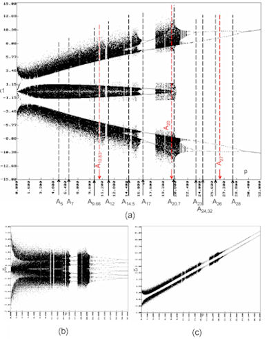
In order to apply SA, the bifurcation diagram (Fig.2) is a useful tool to study the character of the attractors.

In the same figure, the attractors used in achieving the synthesis are plotted together with the synthesized attractors.

3.1 ’Transient attractor’

Numerical simulations of the Rikitake system suggest that the system has attractors which are obviously bounded. In other words, the solutions enter a ball around the origin from which they never escape. However, this seems not to be true, since if we take as an initial condition $(0,0,k)~{}$the exact solution of (1) is $x_{1}(t)=x_{2}(t)=0,$ $x_{3}(t)=t+k$.   But this solution is unstable, the $x_{3}$-axis being an invariant manifold. There are orbits which escape to, or come from, infinity, instead of going towards the attractor. If the flow is on the $x_{3}$-axis it never escapes; if the flow is not on the $x_{3}$-axis, then it can never enter. Because of the mentioned symmetry of solutions, for points arbitrary close to the $x_{3}$-axis, the flow takes the trajectory back to a bounded attractor (results on boundedness of solutions to third-order nonlinear differential equations can be found in [26]).

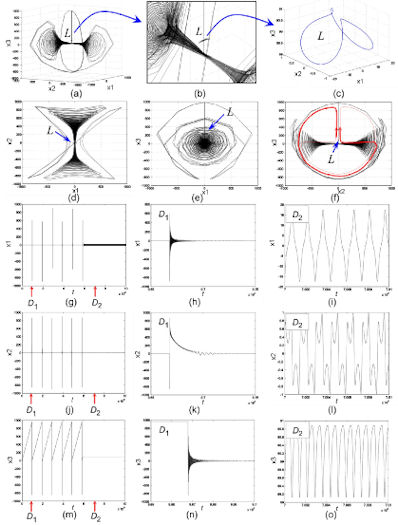
Even though for the above mentioned reasons in some papers the $x_{3}$-axis is regarded as unimportant to the dynamics of the system, we found interesting dynamics due to $x_{3}$-axis instability. Thus, for $p=90,~{}\$we have found a new and intriguing case which can be considered a kind of ”transient attractor” TA (see Fig.3 (a) where the three-dimensional plot is shown and Fig.3 (d-f) where the phase projections have been drawn). TA is actually only a kind of extremely long time transient (its existence being for $t\leq t^{\prime}~{}$with $t^{\prime}$ close to $6\times 10^{6}$) before the trajectory reaches the ’real’ attractor, a stable limit cycle denoted $L~{}~{}$(see Fig.3 (b) where one can see the limit cycle $L$ whose magnified three-dimensional phase plot is shown in Fig. 5 (c)). The dashed lines in Fig.3 (f) indicate the well-defined movement sense of TA. The periodic characteristics of $L$ can be observed in the three time series, corresponding to $x_{1},$ $x_{2}$ and $x_{3}~{}$depicted in Fig.3 (g), (j) and (m) for $t\in\left[0,10^{6}\right]$. The dashed line indicates the moment $t=t^{\prime},~{}$when $L~{}$is born. The details, $D_{1},~{}$for $t\leq t^{\prime}:$ $~{}t\in\left[9.65\times 10^{5},9.75\times 10^{5}\right]$ are presented in Fig.3 (h), (k) and (n). For $t>t^{\prime},$ the TA transforms into $L~{}.~{}$Magnified details, $D_{2},~{}$for $t\in\left[7\times 10^{6},7.1\times 10^{6}\right]~{}$are presented in Fig.3 (i),(l),(o))$.~{}$Before TA ends in $L$, it crosses it several times. It can be seen that the size of TA is of the order of $10^{3}$ as compared to the small size of the $L$ which is nearly $1000$ times smaller. Because a part of the trajectory lies on the $x_{3}$-axis (or is very close to it (see e.g. Fig.3 (d),(e),(f)), the distance being in this case not highlighted by the numerical method), we suspect that the TA appears because of $x_{3}$-axis instability. On this path along the $x_{3}$-axis, the speed of the TA is very slow as compared to the loop speed (see the vertical peeks in the time series in Fig.3 (g),(j),(m) and the details $D_{1}~{}$in Fig.3 (h),(k),(n)). Being a stiff system, not all numerical methods have proved to be adequate to obtain the TA. However, the many simulations and the TA geometric symmetry, encouraged us to consider TA as being not just some ”false” trajectory due to numerical integration, but a real representative component of the insight dynamics of the Rikitake system.

3.2 Attractors synthesis

By applying the deterministic or random SA, any attractor of Rikitake’s system may be synthesized. The standard Runge-Kutta method has been utilized and the most representative cases has been considered. Thus, $\mathcal{P}_{N}$ has been chosen so that all kind of behaviors (regular and chaotic) may be considered.

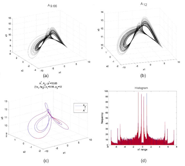
Using the deterministic scheme $[1p_{1},1p_{2}]$ with $p_{1}=9.66$ and $p_{2}=12$, one obtains the synthesized attractor $A^{\ast}$(Fig.4 (c)). Fig.4 (a) and (b) present $A_{p_{1}}$ and $A_{p_{2}}$. $A^{\ast}$ is identical with $A_{p^{\ast}}$ for $p^{\ast}$ given by (8) $p^{\ast}=\left(p_{1}+p_{2}\right)/2=10.83$ (see Fig.4 (c) where both $A^{\ast}$ and$~{}A_{p^{\ast}}$ are plotted superimposed and Fig.4 (d) where histograms of both attractors are presented). It should be noticed that, in this case, SA can be viewed as control algorithm (see Remark 9 i) since $A_{p_{1}}$ and $A_{p_{2}}$ are chaotic and $A^{\ast}$ is a stable limit cycle (see Fig.2).

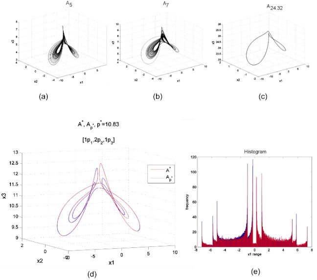
An attractor can be obtained within several variants of (7). For example $A_{10.83}$ synthesized bellow, can be obtained too with the scheme $[1p_{1},2p_{2},1p_{3}]$ with $p_{1}=5,$ $p_{2}=7$ and $p_{3}=24.32~{}$(see Fig.2 and Fig.5). Here, $p^{\ast}=10.83=(p_{1}+2p_{2}+p_{3})/4.$ $A^{\ast}$ and $A_{p^{\ast}}$ are plotted superimposed in Fig.5 (d). Superimposed histograms (Fig.5 (e)) underline the identity.

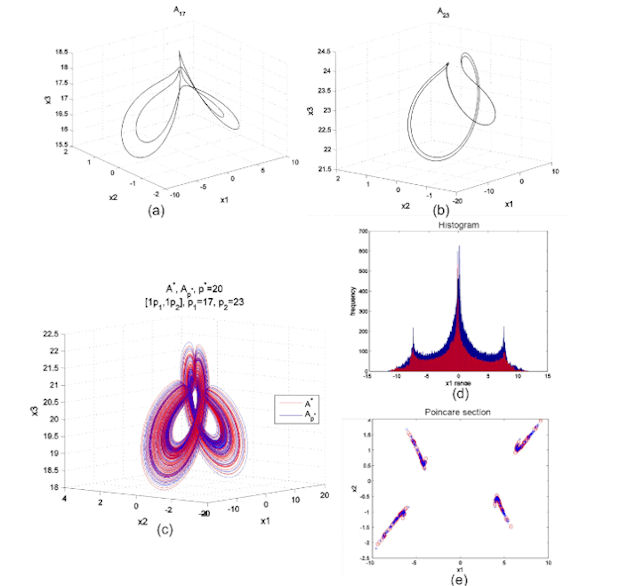
With the scheme $[1p_{1},1p_{2}]$ with $p_{1}=17~{}$and $p_{2}=23$ the chaotic attractor $A^{\ast},$ which is identical to $A_{p^{\ast}}$ with $p^{\ast}=20$ (Fig.2 and Fig.6 (c)), can be obtained. Superimposed histograms and the Poincaré section (Fig.6 (d),(e)) demonstrate the identity. Here SA could be considered as an anticontrol algorithm (see Remark 9 i).

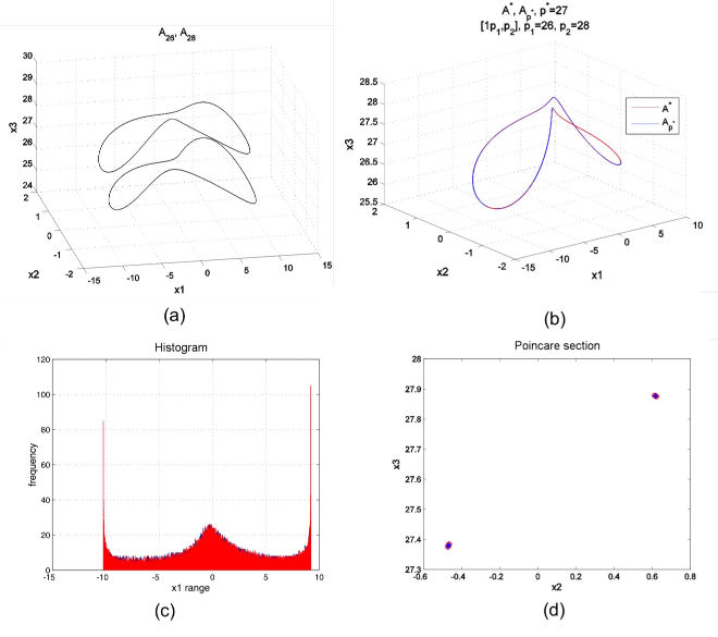
If between $p_{1}$ and $p_{2},$ corresponding to stable attractors, there are no chaotic windows, anticontrol cannot be realized (Remark 9 i). For example, by choosing $p_{1}=26$ and $p_{2}=28$ for which $A_{p_{1}}$ and $A_{p_{2}}$ are stable limit cycles (see Fig.2 and Fig.7 (a) where both attractors are plotted together), whatever kind of scheme (7) is used, only stable limit cycle can be obtained. For example, with the $p_{1,2\text{ }}$chosen bellow, and the scheme $[1p_{1},2p_{2}]~{}$one obtains the limit cycle depicted in Fig.7 (b). The identity between $A^{\ast}$ and $A_{p^{\ast}}$ with $p^{\ast}=27$ is underlined by histograms and Poincaré sections superimposed in Fig.7(d) and (e).

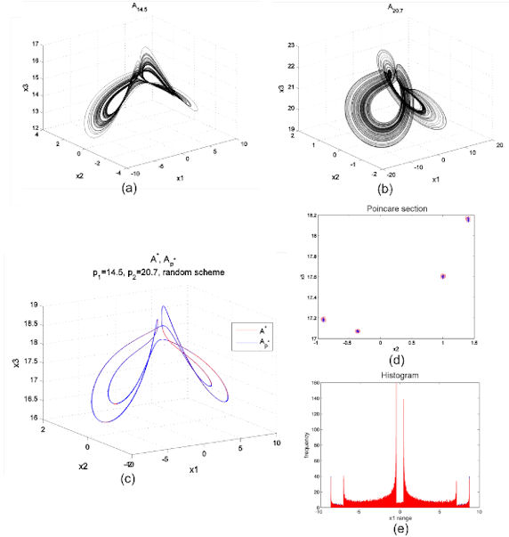
As stated in Section 2, attractors can be synthesized by using random SA. Thus, by choosing the uniform random distribution with algorithm presented in Table 2, for $p_{1}=14.5$ and $p_{2}=20.7,$ one obtains $A^{\ast}$ identical with $A_{p^{\ast}}$ with $p^{\ast}=17.6~{}\$given by (9) (Fig.2 and Fig.8(c)).

The results are presented in Table 3.

4 Conclusions and further directions

In this paper we verified numerically and computationally that any attractor of the Rikitake system can be obtained with the SA, following some deterministic or random rule, the analytical proof being presented in [12].

In addition to the fact that the SA may force the system to evolve along any attractor, it introduces a convex structure inside the attractors set.

Also, SA may serve as a model to explain the born of specific dynamics in systems encountered in the real world or in experiments where this kind of deterministic or random parameter switches may occur.

In this study we extended the application of the SA from systems with hyperbolic equilibrium to systems with non-hyperbolic ones. We have also found an interesting transient attractor, TA, which persists for a long period of time. Its presence is supposed to be due to the instability along the $x_{3}$-axis, and not all numerical methods for ODEs can reveal it. Representing an interesting component of Rikitake’s dynamics, the TA worth to be studied rigorously, for example from the point of view of shadowing theory.

The rigorous proof of the existence of the bijection between the set of parameter values and the set of attractors and the analytical proof of the application of the SA to other class of systems represent tasks for future studies.

Table 1: Pseudo-code of the PS algorithm

repeat

for $i=1$ to $m_{1}$ do

integrate (2) for $p=p_{{}_{1}}$

$t=t+h$

end

…

for $i=1$ to $m_{N}$ do

integrate (2) for $p=p_{{}_{N}}$

$t=t+h$

end

until $t\geq T_{\max}$

Table 2: Pseudo-code of the random PS algorithm

repeat

label=$\operatorname{rand}(N)$

if $label=1$ then

integrate (2) with $p=p_{{}_{1}}$

$m_{1}^{\prime}=m_{1}^{\prime}+1$

if $label=2$ then

integrate (2) with $p=p_{{}_{2}}$

$m_{2}^{\prime}=m_{2}^{\prime}+1$

⋮

if $label=N$ then

integrate (2) with $p=p_{N}$

$m_{N}^{\prime}=m_{N}^{\prime}+1$

$t=t+h$

until $t\geq T_{\max}$

Table 3: The results of PS algoritm applied to the Rikitake system (1)

Scheme	p1	p2	p3	p∗	Remarks
[1p1,1p2]	9.66	12	-	10.83	A${}_{p_{1}}$, A${}_{p_{2}}$ chaotic, A∗ stable limit cycle (Fig.4)
[1p1,2p${}_{2},$,1p3]	5	7	24.32	10.83	A${}_{p_{1}},$ A${}_{p_{2}}~{}$chaotic, A${}_{p_{2}}$stable limit cycle, A∗ stable limit cycle (Fig.5)
[1p1,1p2]	17	23	-	20	A${}_{p_{1}},$ A${}_{p_{2}}~{}$stable limit cycles, A∗ chaotic (Fig.6)
[1p1,1p2]	26	28	-	27	A${}_{p_{1}}$,  A${}_{p_{2}}$stable limit cycles, A∗ stable limit cycle (Fig.7 )
random SA	14.5	20.7	-	17.6	A${}_{p_{1}}$, A${}_{p_{2}}$ chaotic attractors, A∗ stable limit cycle (Fig.8)

Figure 1: Rikitake dynamo (sketch).

Figure 2: Bifurcation diagram for the Rikitake system. (a) Bifurcation diagram for the component $x_{1}$ where the positions of the attractors utilized and the synthesized attractors are indicated; (b), (c) Bifurcation diagram for components $x_{2}$ and $x_{3}$.

Figure 3: Transient attractor (TA) and stable limit cycle L. (a) Phase plot; (b) detail; (c) Limit cycle L after neglected TA; (d), (e), (f) projections of TA and L; (g) Time series for $x_{1}~{}$component; (h), (i) the details $D_{1}$ and $D_{2}$ indicated in (g); (j) Time series for component $x_{2}$; (k),(l) details $D_{1}$ and $D_{2}$ indicated in (j); (m) Time series for component $x_{3}$; (n),(o) Details $D_{1}$ and $D_{2}$ indicated in (m).

Figure 4: Synthesized attractor $A^{\ast}$ and $A_{p^{\ast}}$ obtained with scheme $[1p_{1},1p_{2}]$ with $p_{1}=9.66$ and $p_{2}=12$; $p^{\ast}=10.83.$ (a), (b) Phase plots of $A_{p_{1}}$ and $A_{p_{2}};~{}$(c) $A^{\ast}$ and $A_{p^{\ast}}$ superimposed; (d) Histograms superimposed.

Figure 5: Synthesized attractor $A^{\ast}$ and $A_{p^{\ast}}$ obtained with scheme $[1p_{1},2p_{2},1p_{3}]$ with $p_{1}=5,$ $p_{2}=7,~{}p_{3}=24.32$; $p^{\ast}=10.83.$ (a)-(c) Phase plots of $A_{p_{1,2,3}}.$ (d) $A^{\ast}$ and $A_{p^{\ast}}$ superimposed; (e) Histograms superimposed.

Figure 6: Synthesized attractor $A^{\ast}$ and $A_{p^{\ast}}$ obtained with scheme $[1p_{1},1p_{2}]$ with $p_{1}=17,$ $p_{2}=23$; $p^{\ast}=20.~{}$ (a), (b) Phase plots of $A_{p_{1}}$ and $A_{p_{2}};~{}$(c) $A^{\ast}$ and $A_{p^{\ast}}$ superimposed; (d) Histograms superimposed; (e) Poincaré sections superimposed.

Figure 7: Synthesized attractor $A^{\ast}$ and $A_{p^{\ast}}$ obtained with scheme $[1p_{1},1p_{2}]$ with $p_{1}=26,$ $p_{2}=28$; $p^{\ast}=27.~{}$(a) Phase plots of $A_{p_{1}}$ and $A_{p_{2}}$; (b) $A^{\ast}$ and $A_{p^{\ast}}$ superimposed; (c) Histograms superimposed; (d) Poincaré sections superimposed.

Figure 8: Synthesized attractor $A^{\ast}$ and $A_{p^{\ast}}$ obtained with random scheme with $p_{1}=14.5,$ $p_{2}=20.7;$ $p^{\ast}=17.6.$ (a), (b) Phase plots of $A_{p_{1}}$ and $A_{p_{2}};~{}$(c) $A^{\ast}$ and $A_{p^{\ast}}$ superimposed; (d) Poincaré sections superimposed; (e) Histograms superimposed.

References

- [1] M.-F. Danca, W.K.S. Tang and G. Chen, A switching scheme for synthesizing attractors of dissipative chaotic systems, Appl. Math. Comput. 201 (1-2) (2008), pp. 650-667.
- [2] G.A. Glatzmaier, R.S. Coe, L. Hongre and P.H. Roberts, The role of the Earth’s mantle in controlling the frequency of geomagnetic reversals, Nature 401 (1999), pp. 885-890.
- [3] G.A. Glatzmaier and P.H. Roberts, A three-dimensional self-consistent computer simulation of a geomagnetic field reversal, Nature 377 (1995), pp. 203-209.
- [4] T. Rikitake, Oscillations of a system of disk dynamos, P. Cambridge Philos. Soc. 54 (1958), pp. 89-105.
- [5] D.R.J. Chillingworth and P.J. Holmes, Dynamical systems and models for the reversals of the Earth’s magnetic field, Math. Geol. 12 (1) (1980), pp. 41-59.
- [6] R. Hide, A.C. Skeldon and D.J. Acheson, A study of two novel self-exciting single-disk homopolar dynamos: theory, P. Roy. Soc. A-Math. Phy. 452 (1996), pp. 1369-1395.
- [7] B.A. Buffett, Earth’s Core and the Geodynamo, Science 288 (5473) (2000), pp. 2007-2012.
- [8] P. Hoyng, D. Schimtt and M.A.J.H. Ossendrijver, A theoretical analysis of the observed variability of the geomagnetic dipole field, Phys. Earth Planet. Inter. 130 (3-4) (2002), pp. 143-157.
- [9] A.E. Cook and P.H. Roberts, The Rikitake two-disc dynamo system, Math. Proc. Cambridge 68 (02) (1970), pp. 547-569.
- [10] J. Llibre and M. Messias, Global dynamics of the Rikitake system, Physica D 238 (3) (2009), pp. 241-252.
- [11] F. Plunian, P. Marty and A. Alemany, Chaotic behavior of the Rikitake dynamo with symmetric mechanical friction and azimuthal currents, P. Roy. Soc. A-Math. Phy. 454 (1998), pp. 1835-1842.
- [12] Y. Mao, W.K.S. Tang and M.-F. Danca, An Averaging Model for the Chaotic System with Periodic Time-Varying Parameter, Appl. Math. Comput. 217 (1) (2010), pp. 355-362.
- [13] J.A. Sanders and F. Verhulst, Averaging Methods in Nonlinear Dynamical Systems, Springer-Verlag, New York (1985).
- [14] M.-F. Danca and K. Diethlem, Fractional-order attractors synthesis via parameter switchings, Commun. Nonlinear Sci. Numer. Simulat. 15 (12) (2010), pp. 3745–3753.
- [15] X. Wu, J. Li and G. Chen, Chaos in the fractional order unified system and its synchronization, J. Frank. Inst. 345 (4) (2008), pp. 392-401.
- [16] B.A. Coombes, H. Kocak and K.J. Palmer, Rigorous computational shadowing of orbits of ordinary differential equations, Numer. Math. 69 (4) (1995), pp. 401-421.
- [17] L. Kapitanski and I. Rodnianski, Shape and Morse theory of attractors, Comm. Pure Appl. Math. 53 (2) (2000), pp. 218-242.
- [18] M.W. Hirsch, S. Smale and R.L. Devaney, Differential Equations. Dynamical Systems and An Introduction to Chaos and an Introduction to Chaos 2nd ed. Elsevier Academic Press, London, (2004).
- [19] C. Foias and M.S. Jolly, On the numerical algebraic approximation of global attractors, Nonlinearity 8 (3) (1995), pp. 295
- [20] A. Oksasoglu and Q. Wang, Rank one Chaos in a switch-controlled Chua’s circuit, J. Frank. Inst. (2010) in press.
- [21] M.-F. Danca, Random parameter-switching synthesis of a class of hyperbolic attractors, Chaos 18 (2008), 033111.
- [22] M. J. Ogorzalek, Chaos control: How to avoid chaos or take advantage of it, J. Frank. Inst. 331 (6) (1994), pp. 681-704.
- [23] C. Grebogi, Y.C. Lai, and S. Hayes, Control and applications of chaos, J. Frank. Inst. 334 (5-6) (1997), 1115-1146.
- [24] G. Chen and Y. Shi, Introduction to anti-control of discrete chaos: theory and applications, Phil. Trans. R. Soc. A 364 (2006), pp. 2433–2447.
- [25] X. F. Wang, Generating chaos in continuous-time systems via feedback control, in Chaos control: Theory and applications, Lecture Notes in Control and Information Science, G. Chen and X. Xu eds. 292 (2004), pp. 179-204.
- [26] C. Tunç, Bound of solutions to third-order nonlinear differential equations with bounded delay, J. Frank. Inst. 347 (2) (2010), pp. 415-425.