Armchair graphene nanoribbons: $\mathcal{PT}$-symmetry breaking
and exceptional points without dissipation

Abstract

We consider a single-layer graphene nanoribbon with armchair edges and with a longitudinally constant external potential, pointing out that it can be described by means of an effective non-Hermitian Hamiltonian. We show that this system has some features typical of dissipative systems, namely the presence of exceptional points and of $\mathcal{PT}$-symmetry breaking, although it is not dissipative.

Since its isolation in 2004 Novoselov04 , graphene has attracted a significant interest in the condensed matter community because of its unique electronic properties, the most astonishing one being the presence in its low-energy spectrum of two massless Dirac modes. These massless fermionic excitations allowed the experimental observation of exotic phenomena, such as the Klein paradox and the Zitterbewegung (see e.g. CastroNeto for a review), theoretically studied in the context of quantum electrodynamics long before.

In this letter we analyze some properties of single-layer graphene nanoribbons with armchair edges in an external potential, pointing out a connection with the recently developed theory of $\mathcal{PT}$-symmetric non-Hermitian Hamiltonians in quantum mechanics.

The systematic study of $\mathcal{PT}$-symmetric Hamiltonians was initiated by the seminal paper Bender98 , in which analytical and numerical hints were presented to explain the reality of the spectra of some non-Hermitian Hamiltonians. If the $\mathcal{PT}$ symmetry is realized in the spectrum, i.e. if every eigenstate of the Hamiltonian is also an eigenstate of the $\mathcal{PT}$ operator, it is simple to show that the energy spectrum has to be real. However, since $\mathcal{PT}$ is an anti-linear operator, the symmetry can be spontaneously broken (for some enlightening examples and a review of the main results obtained in this field see e.g. Bender07 ) and EPs (exceptional points) can appear. Exceptional points, i.e. points for which two (or more) eigenvalues coalesce and the Hamiltonian is non-diagonalizable Kato , are a typical feature of non-Hermitian Hamiltonians (see e.g. the reviews EP ) with no Hermitian counterpart and they have been shown to produce experimentally observable effects mw ; EP_exp1 ; EP_exp2 .

To our knowledge, all the previously proposed physical examples of systems governed by non-Hermitian $\mathcal{PT}$-symmetric Hamiltonians involve dissipative systems, the main emphasis being on microwave cavities mw , optical lattices optic_th ; optic_exp and lasers laser . We show that, because of the spinorial nature of the wave function, some properties of graphene nanoribbons can be described by means of an effective non-Hermitian $\mathcal{PT}$-symmetric Hamiltonian, although there is no dissipation. We give numerical evidence for the $\mathcal{PT}$-symmetry breaking and provide an order parameter. Finally we study the behavior of eigenmodes and eigenfunctions in the neighborhood of exceptional points.

The model and the notations.

We consider a nanoribbon section with open boundary conditions along the longitudinal $x$ direction, armchair edges, and $N$ dimer lines across its width. The transverse distance (along the $y$ direction) between the first line of lattice points not occupied by carbon atoms at the bottom edge and the analogous one at the upper edge of the ribbon (i.e. the “effective width” of the ribbon) is equal to $L=(N+1)a/2$, with $a$ the graphene lattice constant. The wave function is equal to

$$\psi(\vec{r})=\sum_{\vec{R}_{A}}\psi_{A}(\vec{R}_{A})\varphi(\vec{r}-\vec{R}_{A})+i\sum_{\vec{R}_{B}}\psi_{B}(\vec{R}_{B})\varphi(\vec{r}-\vec{R}_{B})\,,$$ (1)

where the $\varphi(\vec{r})$’s are the orthonormalized $2p^{z}$ atomic orbitals of carbon, $\vec{R}_{A}$ and $\vec{R}_{B}$ are the positions of the atoms of the two sublattices $A$ and $B$ of graphene, and

$$\vec{\Psi}(\mathbf{r})=\begin{pmatrix}\psi_{A}(\mathbf{r})\\ \psi_{B}(\mathbf{r})\end{pmatrix}=e^{-iKy}\vec{\chi}^{\vec{K}}(x,y)-e^{iKy}\vec{\chi}^{\vec{K}^{\prime}}(x,y)\,,$$ (2)

with $K=4\pi/(3a)$ and $\vec{\chi}^{\vec{K}}$, $\vec{\chi}^{\vec{K}^{\prime}}$ the $2$-spinors corresponding to the two inequivalent Dirac points $\vec{K}$ and $\vec{K}^{\prime}$. The external potential $V(x,y)$ is assumed to vary only in the transverse direction. Aside from its intrinsic interest, evaluation of the eigenfunctions and eigenvalues for such a potential represents the first step in conductance calculations for a generic potential (varying in both spatial directions) performed by means of scattering matrix methods. Most existing calculations of transport in graphene based on such methods deal instead with a constant transverse potential wurm ; li .

We can expand $\vec{\chi}^{\vec{K}}$, $\vec{\chi}^{\vec{K}^{\prime}}$ in plane waves along the $x$ direction and write $\vec{\chi}^{\vec{K}}(x,y)=e^{ik_{x}x}\vec{\varphi}^{\vec{K}}(y)$ and $\vec{\chi}^{\vec{K}^{\prime}}(x,y)=e^{ik_{x}x}\vec{\varphi}^{\vec{K}^{\prime}}(y)$. The Dirac equation can be written in the form (see e.g. bc ; CastroNeto )

$$\left\{\begin{aligned} &\big{(}f(y)+\sigma_{x}k_{x}-i\sigma_{y}\partial_{y}\big{)}\vec{\varphi}^{\vec{K}}(y)=0\\ &\big{(}f(y)+\sigma_{x}k_{x}+i\sigma_{y}\partial_{y}\big{)}\vec{\varphi}^{\vec{K}^{\prime}}(y)=0\end{aligned}\right.$$ (3)

where we introduced the shorthand $f(y)=[V(y)-E]/v_{F}$, with $v_{F}$ the Fermi velocity (we use $\hbar=1$ in order to simplify the notations), and the armchair boundary conditions read

$$\vec{\varphi}^{\vec{K}}(0)=\vec{\varphi}^{\vec{K}^{\prime}}(0)\ ,\quad\vec{\varphi}^{\vec{K}}(L)=e^{2ikL}\vec{\varphi}^{\vec{K}^{\prime}}(L).$$ (4)

The $k_{x}$ values for which this system admits non trivial solutions are the longitudinal momenta allowed in the nanoribbon. The problem of Eqs. (3)-(4) can be rewritten in a more convenient form introducing, for $y\in[-L,L]$, the $2$-spinor

$$\vec{\varphi}(y)=\begin{cases}\vec{\varphi}^{\vec{K}}(y+L)&y\in[-L,0]\\ e^{2iKL}\,\vec{\varphi}^{\vec{K}^{\prime}}(L-y)&y\in]0,L]\end{cases}$$ (5)

and defining $\bar{f}(y)=f(L-|y|)$ and $H^{k_{x}}(y)=\bar{f}(y)\sigma_{y}-ik_{x}\sigma_{z}$. We obtain

$$i\partial_{y}\vec{\varphi}(y)=H^{k_{x}}(y)\vec{\varphi}(y),\quad\vec{\varphi}(L)=e^{2iKL}\vec{\varphi}(-L),$$ (6)

which is formally equivalent to a Schrödinger equation for the non-Hermitian Hamiltonian $v_{F}H^{k_{x}}$, if we interpret $y/v_{F}$ as the time.

Symmetries.

From Eq. (6) we deduce a simple result on the degeneration of the $k_{x}$ modes. If we denote by $U(y)$ the time evolution operator associated to a given eigenvalue $k_{x}$, i.e. $\vec{\varphi}(y)=U(y)\vec{\varphi}(-L)$ with $\vec{\varphi}(y)$ in the corresponding eigenspace, the boundary condition can be written as $U(L)\vec{\varphi}(-L)=e^{2iKL}\vec{\varphi}(-L)$. By using the explicit form of $H^{k_{x}}$ it is easy to check that $U^{-1}(L)=\sigma_{x}U(L)\sigma_{x}$, from which it follows that $U(L)\sigma_{x}\vec{\varphi}(-L)=e^{-2iKL}\sigma_{x}\vec{\varphi}(-L)$. If $\exp(4iKL)\neq 1$, there cannot be eigenvectors of $U(L)$ other than $\vec{\varphi}(-L)$ and $\sigma_{x}\vec{\varphi}(-L)$, and hence just one independent eigenmode corresponds to each $k_{x}$. From now on we consider lengths $L$ for which this condition is verified, i.e. nanoribbons that are semiconducting in the absence of an external potential also when edge relaxation is neglected. We denote by $\vec{\varphi}_{k_{x}}(y)$ the eigenmode associated to $k_{x}$. From the relations

$$\vec{\varphi}_{k_{x}^{*}}(y)\sim\sigma_{x}\bigl{(}\vec{\varphi}_{k_{x}}(-y)\bigr{)}^{*} \vec{\varphi}_{-k_{x}^{*}}(y)\sim\sigma_{z}\bigl{(}\vec{\varphi}_{k_{x}}(-y)\bigr{)}^{*}$$ (7)

it follows that if $k_{x}$ is in the spectrum then there are also $k_{x}^{*}$, $-k_{x}^{*}$ and $-k_{x}$. Thus the spectrum has a $Z_{2}\times Z_{2}$ symmetry.

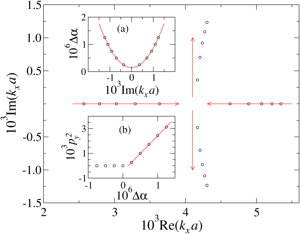
Figure 1: Coalescing of two eigenvalues along the real line for $\epsilon=1/5$; the arrows denote the direction of increasing $\alpha$ values ($\Delta\alpha\equiv\alpha-0.060953$). In the inset (a) the imaginary parts of the coalescing eigenvalues are shown together with a fit of the form $\alpha=c_{1}+c_{2}(\mathrm{Im}\,(k_{x}a))^{2}$. The inset (b) shows the behavior of the square of the transverse momentum together with a linear fit.

To reveal the $\mathcal{PT}$ symmetry of this problem it is convenient to take the square of Eq. (6) and project $\vec{\varphi}$ on the eigenstates of $\sigma_{y}$. If we denote these projections by $\phi_{\pm}$, they satisfy the equations

$$\Big{(}\hat{p}_{y}^{2}-\bar{f}^{\,2}\mp i(\partial_{y}\bar{f})\Big{)}\phi_{\pm}(y)=-k_{x}^{2}\phi_{\pm}(y),$$ (8)

which are clearly invariant under the $\mathcal{PT}$ transformation, being the action of the operators $\mathcal{P}$ and $\mathcal{T}$ defined by $p_{y}\rightarrow-p_{y}$, $y\rightarrow-y$ and $p_{y}\rightarrow-p_{y}$, $y\rightarrow y$, $i\rightarrow-i$, respectively. If the $\mathcal{PT}$ symmetry is unbroken then $k_{x}$ has to be real or imaginary; complex conjugate (intended here as a number with nonzero real and imaginary part) pairs appear in the spectrum only if this symmetry is broken.

We explicitly notice that if the Schrödinger equation is used instead of the Dirac one, the equation corresponding to Eqs. (3) is similar to Eq. (8) but with an Hermitian left hand side, so that all the $k_{x}$ values have to be real or imaginary.

In the presence of spontaneously broken symmetries it is customary to look for an order parameter, i.e. an observable that vanishes when the symmetry is realized in the spectrum, a non zero value signaling the symmetry breaking. We point out that the mean value of the transverse momentum

$$p_{y}=\left.\int_{0}^{L}\vec{\Psi}(y)^{{\dagger}}(-i\partial_{y})\vec{\Psi}(y)\mathrm{d}y\right/\int_{0}^{L}\vec{\Psi}(y)^{{\dagger}}\vec{\Psi}(y)\mathrm{d}y$$ (9)

satisfies this requirement. This can be easily proved exploiting the symmetries of our problem: from Eqs. (7) and because $|\vec{\varphi}(y)|^{2}$ is $\mathcal{P}$-even and $\vec{\varphi}(-y)^{T}\sigma_{z}\vec{\varphi}(y)$ is constant, it follows that the numerator of Eq. (9) vanishes if $k_{x}^{2}$ is real. We checked numerically that the transverse momentum $p_{y}$ is different from zero when $k_{x}$ is complex ($p_{y}$ appears to vanish also for complex $k_{x}$ values only when the potential satisfies $V(y)=V(L-y)$). Thus, in this system the realization of the $\mathcal{PT}$ symmetry in the spectrum is related to the value of the transverse momentum, which is an order parameter for the $\mathcal{PT}$ symmetry breaking. This is completely analogous to what happens in QCD with compact dimensions, when charge conjugation can get spontaneously broken and the related order parameter is the baryon current in the compactified direction lpp .

Finally, it is worth mentioning that the transformation that reverses the sign of $\bar{f}(y)$ (i.e. $\sigma_{z}$) is unitary and independent of $p_{y}$, and hence $|\vec{\varphi}(y)|^{2}$ is invariant for simultaneous flipping of the signs of the potential and of the energy. This is just a manifestation of the chiral symmetry of the system. As long as $\bar{f}(y)$ does not have a definite sign, heuristic arguments based on that symmetry indicate the presence of eigenfunctions localized around the minima as well as eigenfunctions localized around the maxima of the potential; the former (latter) ones are expected to describe particles with positive (negative, i.e. of opposite sign with respect to $k_{x}$) group velocities. These observations provide a simple argument for the existence of some singular behavior: by varying the energy, eigenmodes with opposite group velocities coalesce in a non-analytic way, because they cannot combine in a two-dimensional eigenspace.

$\mathcal{PT}$-symmetry breaking and exceptional points

If $f(y)$ is constant, Eq. (6) can be analytically solved: all the $k_{x}$ values are real or imaginary and all the eigenstates of the Hamiltonian (their projections on the eigenstates of $\sigma_{y}$, to be precise) are also eigenstates of the $\mathcal{PT}$ operator. This is no longer true when an external potential with non-trivial $y$ dependence is present and we now provide numerical evidence that in this system $\mathcal{PT}$-symmetry can get spontaneously broken. As a simple example we use the Lorentzian shaped potential

$$f(y)\,a=\epsilon-\frac{125}{250+\alpha^{2}((y/a)-150)^{2}},$$ (10)

with $\alpha,\epsilon\in\mathbb{R}$. The general qualitative features are however independent of the particular potential adopted. We choose $L=500a$ as the effective width of the nanoribbon.

It is simple to (numerically) check that by varying the parameters ($\alpha$ and $\varepsilon$ in our example) two different phenomena can occur:

• the number of the real eigenvalues varies but the number of the complex ones is preserved;

• the number of the complex eigenvalues changes.

In case A) a couple of real eigenvalues turns into a couple of imaginary ones (or vice versa); the $Z_{2}\times Z_{2}$ symmetry then implies the existence of some values of the parameters for which $k_{x}=0$ is a doubly degenerate eigenvalue. However, we are assuming $\exp(4iKL)\neq 1$, and hence only one independent eigenfunction is associated to each eigenvalue; as a consequence, this point of the parameter space is an exceptional point. Case B) is completely analogous: two real or imaginary eigenvalues coalesce and become complex (see Fig. 1). However, while in case A) the $\mathcal{PT}$ symmetry is unbroken (or broken, if the number of complex eigenvalues is different from $0$) irrespective of the EP, in case B) the EP is associated to $\mathcal{PT}$ symmetry breaking. Clearly this kind of EP appears in a specular way both in the upper (right) and lower (left) half-plane, because of the $Z_{2}\times Z_{2}$ symmetry.

Behavior near EPs.

If we are not at an exceptional point, the variations of the eigenvalues and eigenvectors are linear in the variation $\delta\bar{f}$ of $\bar{f}$; in particular it can be shown that

$$\int_{-L}^{L}\mathrm{d}y\vec{\varphi}^{T}_{k_{x}}(-y)\frac{\delta\bar{f}}{\delta k_{x}}\sigma_{x}\vec{\varphi}_{k_{x}}(y)=-\int_{-L}^{L}\mathrm{d}y\vec{\varphi}^{T}_{k_{x}}(-y)\vec{\varphi}_{k_{x}}(y)\,.$$ (11)

The group velocity $v^{g}_{x}$ in the $x$ direction is obtained in the special case of an energy shift and is given by

$$v^{g}_{x}\equiv\frac{\delta E}{\delta k_{x}}=v_{F}\frac{\int_{-L}^{L}\mathrm{d}y\,\vec{\varphi}^{T}_{k_{x}}(-y)\vec{\varphi}_{k_{x}}(y)}{\int_{-L}^{L}\mathrm{d}y\,\vec{\varphi}^{T}_{k_{x}}(-y)\sigma_{x}\vec{\varphi}_{k_{x}}(y)}\,.$$ (12)

The velocity defined as above has a clear physical interpretation for real modes, for which it is real; however also complex group velocities can provide interesting information in many physical systems (see e.g. Complex_v ).

At an EP, $\int_{-L}^{L}\mathrm{d}y\,\vec{\varphi}^{T}_{k_{x}}(-y)\vec{\varphi}_{k_{x}}(y)$ vanishes for some $k_{x}$ and in the neighborhood of an EP corresponding to the eigenvalue $k_{x}^{EP}$ we find

$$\delta E\cong\frac{(k_{x}-k_{x}^{EP})^{2}}{2\mu},\quad\mu=\frac{1}{v_{F}}\frac{\int_{-L}^{L}\mathrm{d}y\,\vec{\varphi}^{T}_{k_{x}}(-y)\sigma_{x}\vec{\varphi}_{k_{x}}(y)}{\frac{\delta}{\delta k_{x}}\int_{-L}^{L}\mathrm{d}y\,\vec{\varphi}^{T}_{k_{x}}(-y)\vec{\varphi}_{k_{x}}(y)}\,.$$ (13)

This is nothing but the well known square root behavior, in the neighborhood of an EP Kato ; EP , of two coalescing eigenvalues as a function of the external parameters (see the inset (a) of Fig. 1). Near an EP we can then factorize the Hilbert space as the product of the $2d$ space of the collapsing eigenfunctions, for which the $k_{x}$’s rapidly change with a small shift in $E$ (fast modes), and the span of the other modes (slow modes), which can be assumed as fixed in the neighbourhood of the EP. Here we are assuming that eigenfunctions associated to different exceptional points do not mix; in the considered numerical examples we checked that this assumption is indeed true. Thus:

$$\begin{pmatrix}\vec{\varphi}_{k_{x}^{(1)}}\\ \vec{\varphi}_{k_{x}^{(2)}}\end{pmatrix}\approx R\begin{pmatrix}\vec{\varphi}_{+}\\ \vec{\varphi}_{-}\end{pmatrix}\,,$$ (14)

where $k_{x}^{(1)},k_{x}^{(2)}$ are the two coalescing eigenvalues, $R$ is a $2\times 2$ matrix and $\vec{\varphi}_{\pm}$ are the two initial states. Notice that if the difference between one or more eigenvalues and the coalescing ones is $\delta k_{x}\lesssim\mu$, they can mix together. It turns out that if they are quasi-degenerate with the coalescing eigenmodes ($\delta k_{x}\ll\mu$) the mixing between them is just a rotation, that is irrelevant for the features that we are going to describe. As long as we are not at the EP, we can choose the normalization $\int_{-L}^{L}\mathrm{d}\varphi\vec{\varphi}_{k_{x}^{\prime}}^{T}(-y)\vec{\varphi}_{k_{x}}(y)=\delta_{k_{x}k_{x}^{\prime}}$, so that $RR^{T}=\mathrm{I}$. For the sake of simplicity, in the following we restrict to the case of $\delta\bar{f}=-\delta E/v_{F}$ and EPs on the real axis. The qualitative results obtained are nevertheless of general validity. Before the EP is reached, the group velocities of the coalescing real eigenmodes are opposite in sign, as shown by Eq. (13) and indicated by the subscript $\pm$ in Eq. (14), and from Eqs. (7) it follows that $R^{\ast}=\sigma_{z}R\sigma_{z}$. After the EP is crossed, the eigenvalues as well as $\delta E/\delta k_{x}$ become complex conjugate and from Eqs. (7) it follows that $R^{\ast}=\pm\sigma_{x}R\sigma_{z}$. Relaxing the normalization condition, we can parametrize $R$ as follows:

$$R\sim\mathrm{I}+e^{i\theta}\sigma_{y}\,.$$ (15)

The domain of definition of the parameter $\theta$ is $]\infty i,0i]\cup[0,\pi]\cup[\pi+0i,\pi+\infty i[$. The $k_{x}$ values are real if $\mathrm{Im}\,\theta$ is different from $0$ and complex if $\theta$ is real; the larger $\mathrm{Im}(\theta)$ the further apart the modes $k_{x}^{(1,2)}$ are. When $\theta=0$ the eigenfunctions $\vec{\varphi}_{k_{x}^{(1,2)}}$ are linearly dependent, so this value corresponds to an exceptional point. We rewrite Eq. (13) in terms of the parameter $\theta$ in the simplest case in which the term $\Delta\equiv\int_{-L}^{L}\mathrm{d}y\vec{\varphi}_{+}(-y)^{T}\sigma_{x}\vec{\varphi}_{-}(y)$, which appears in $\mu$, is negligible

$$\left\{\begin{aligned} &k_{x}^{(1,2)}\approx k_{x}^{0}+2\mu\frac{(v_{+}^{-1}+v_{-}^{-1})\cos\theta\mp i(v_{+}^{-1}-v_{-}^{-1})\sin\theta}{(v_{+}^{-1}-v_{-}^{-1})^{2}}\\ &E\approx E_{0}-\frac{4\mu}{(v_{+}^{-1}-v_{-}^{-1})^{2}}\cos\theta\,,\end{aligned}\right.$$ (16)

where $k_{x}^{0}$ and $E_{0}$ are constants and $v_{\pm}$ are the group velocities associated to the eigenfunctions $\vec{\varphi}_{\pm}$. The condition $\Delta\approx 0$ is found for example when one eigenfunction is localized around the minima and the other around the maxima of the potential. The approximate Eq. (16) is accurate only in a neighborhood of the EP with $\theta\approx 0$ but, if $\mu$ is much less than the energy scale in which the Hilbert space factorization remains valid, then the value $\theta=\pi$ of Eq. (15) corresponds actually to another EP, and the previous approximation is good in the whole interval $0\leq\theta\leq\pi$. This happens when two real eigenvalues collide, become complex and then come back on the real axis, the two EPs being sufficiently close to each other. In this case Eq. (16) captures the whole out-of-axes “motion” of the eigenvalues. In Fig. 2 the results predicted by Eqs. (15) and (16) are checked against numerical data and the agreement appears to be excellent. After crossing both exceptional points, the eigenfunctions almost return to the starting ones; observe, moreover, that the energy scale of the phenomenon shown in Fig. 2 is of order $\approx 10^{-8}v_{F}/a$, to be compared with an analytical background of order $\approx 0.2v_{F}/a$ (see the caption of Fig 2). These aspects make the numerical observation of the phenomenon extremely difficult, so that the effect of two very close EPs may be incorrectly interpreted as a mode-crossing.

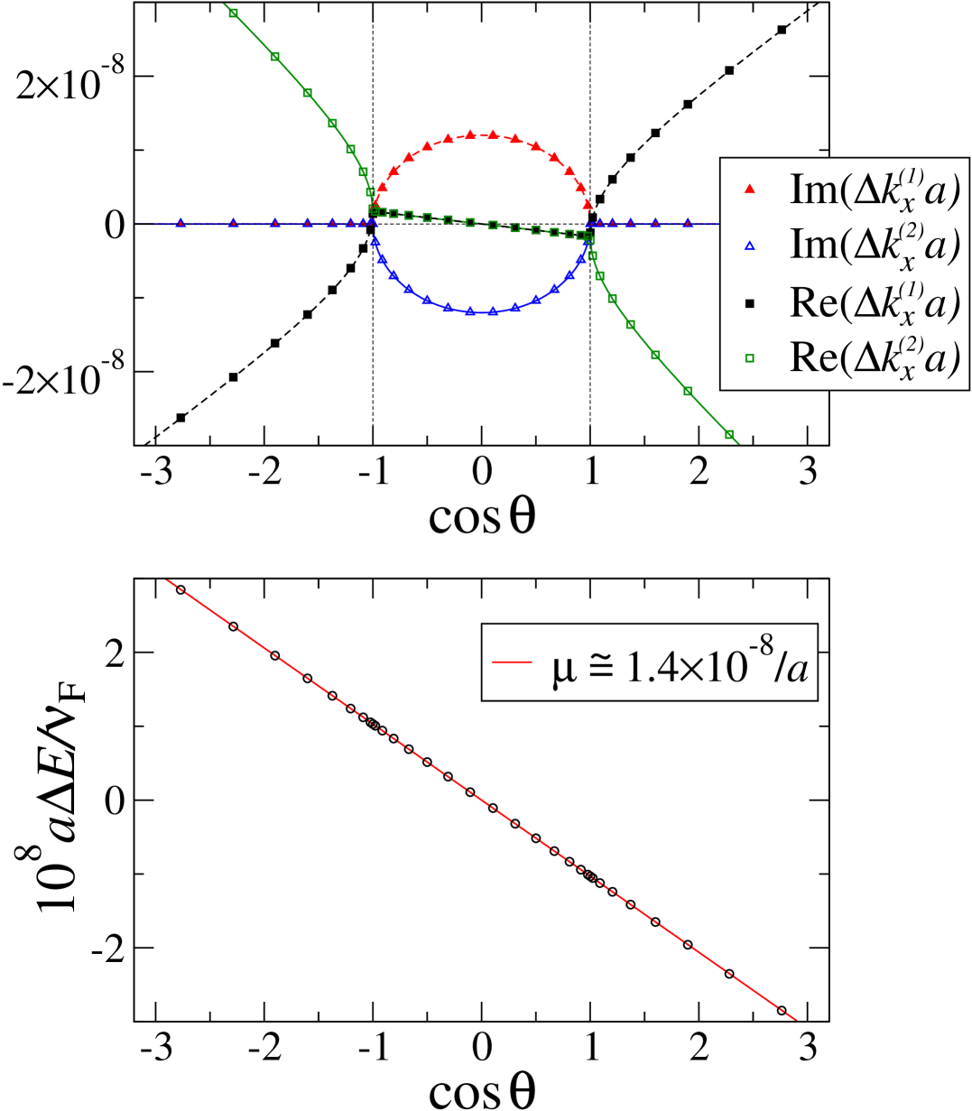
Figure 2: The momenta (top) $\Delta k_{x}^{(1,2)}\approx k_{x}^{(1,2)}-0.199894795/a$ and the energy (bottom) $\Delta E\approx E+0.200651930\,v_{F}/a$ of two coalescing modes as functions of $\cos\theta$, estimated from $(\det R-2)/\sqrt{1-\det R}$ (see Eqs. (14) and (15)), for the potential (10) with $\alpha=\pi/2$ and $\epsilon=-a\,E/v_{F}$. The lines in the upper graph follow the prediction (16): the asymptotic velocities $v_{\pm}$ are obtained by considering $\Delta E\gtrsim 2\cdot 10^{-5}\,v_{F}/a$ and $\mu$ obtained from the linear fit of the energy versus $\cos\theta$ shown in the bottom graph.

Conclusions.

We have pointed out a connection between properties of graphene and the theory of non-Hermitian Hamiltonians, by showing that armchair graphene nanoribbons provide the first example of a nondissipative system described by a $\mathcal{PT}$-symmetric non-Hermitian Hamiltonian. We have also established that the transverse momentum $p_{y}$ is an order parameter for the $\mathcal{PT}$ symmetry breaking. We have numerically verified the presence of exceptional points and shown that, in their neighborhood, the behavior of $p_{x}$ and of the eigenfunctions of the Dirac Hamiltonian, in the presence of a longitudinally invariant external potential, is theoretically well understood.

An aspect that certainly deserves further study is the effect of exceptional points on the transport properties of graphene nanoribbons, in the presence of a potential that varies also in the longitudinal direction. Moreover it would be interesting to study more in depth the properties of complex eigenmodes and the effects of the non-vanishing transverse momentum.

We thank M. D’Elia for useful comments. D. L., M. M., and P. M. gratefully acknowledge support from the EU FP7 IST Project GRAND (contract number 215752) via the IUNET consortium.

References

- (1) K. S. Novoselov et al., Science 306, 666 (2004) [arXiv:cond-mat/0410550].
- (2) A. H. Castro Neto et al., Rev. Mod. Phys. 81, 109 (2009) [arXiv:0709.1163].
- (3) C. M. Bender and S. Boettcher, Phys. Rev. Lett. 80 , 5243 (1998) [arXiv:physics/9712001].
- (4) C. M. Bender, Rep. Prog. Phys. 70, 947 (2007) [arXiv:hep-th/0703096].
- (5) T. Kato Perturbation Theory for Linear Operators (Springer, Berlin, 1995).
- (6) M. V. Berry, Czech. J. Phys 54, 1039 (2004); W. D. Heiss, Czech. J. Phys 54, 1091 (2004).
- (7) C. Dembowski et al., Phys. Rev. Lett. 86, 787 (2001); C. Dembowski et al., Phys. Rev. Lett. 90, 034101 (2003) [arXiv:nlin/0212023]; S.-B. Lee et al., Phys. Rev. Lett. 103, 134101 (2009) [arXiv:0905.4478].
- (8) H. Cartarius et al., Phys. Rev. Lett. 99, 173003 (2007) [arXiv:nlin/0703023].
- (9) S. Klaiman et al., Phys. Rev. Lett. 101, 080402 (2008) [arXiv:0802.2457]; A. Mostafazadeh, Phys. Rev. Lett. 102, 220402 (2009) [arXiv:0901.4472].
- (10) R. El-Ganainy et al., Opt. Lett. 32, 2632 (2007); Z. H. Musslimani et al., Phys. Rev. Lett. 100, 030402 (2008); K. G. Makris et al., Phys. Rev. Lett. 100, 103904 (2008).
- (11) A. Guo et al., Phys. Rev. Lett. 103, 093902 (2009); C. E. Rüter et al., Nature Phys. 6, 192 (2010).
- (12) H. Schomerus, Phys. Rev. Lett. 104, 233601 (2010) [arXiv:1001.0539]; Y. D. Chong et al., Phys. Rev. Lett. 105, 053901 (2010) [arXiv:1003.4968].
- (13) J. Wurm et al., New J. Phys. 11, 095022 (2009).
- (14) H. Liet al., Phys. Rev. B 79, 155429 (2009) [arXiv:0906.4351].
- (15) L. Brey and H. A. Fertig, Phys. Rev. B 73, 235411 (2006) [arXiv:cond-mat/0603107].
- (16) B. Lucini et al., Phys. Rev. D 75, 121701(R) (2007) [arXiv:hep-th/0702167].
- (17) V. Gerasik and M. Stastna, Phys. Rev. E 81, 056602 (2010).