Magnetic Cycles in a Convective Dynamo Simulation of a Young Solar-type Star

Abstract

Young solar-type stars rotate rapidly and many are magnetically active. Some appear to undergo magnetic cycles similar to the 22-year solar activity cycle. We conduct simulations of dynamo action in rapidly rotating suns with the 3D MHD anelastic spherical harmonic (ASH) code to explore dynamo action achieved in the convective envelope of a solar-type star rotating at 5 times the current solar rotation rate. We find that dynamo action builds substantial organized global-scale magnetic fields in the midst of the convection zone. Striking magnetic wreaths span the convection zone and coexist with the turbulent convection. A surprising feature of this wreath-building dynamo is its rich time-dependence. The dynamo exhibits cyclic activity and undergoes quasi-periodic polarity reversals where both the global-scale poloidal and toroidal fields change in sense on a roughly 1500 day time scale. These magnetic activity patterns emerge spontaneously from the turbulent flow and are more organized temporally and spatially than those realized in our previous simulations of the solar dynamo. We assess in detail the competing processes of magnetic field creation and destruction within our simulations that contribute to the global-scale reversals. We find that the mean toroidal fields are built primarily through an $\Omega$-effect, while the mean poloidal fields are built by turbulent correlations which are not necessarily well represented by a simple $\alpha$-effect. During a reversal the magnetic wreaths propagate towards the polar regions, and this appears to arise from a poleward propagating dynamo wave. As the magnetic fields wax and wane in strength and flip in polarity, the primary response in the convective flows involves the axisymmetric differential rotation which varies on similar time scales. Bands of relatively fast and slow fluid propagate towards the poles on time scales of roughly 500 days and are associated with the magnetic structures that propagate in the same fashion. In the Sun, similar patterns are observed in the poleward branch of the torsional oscillations, and these may represent poleward propagating magnetic fields deep below the solar surface.

1. Introduction

Motivated by the rich observational landscape of stellar magnetism and by our own Sun’s cycles of activity, we have undertaken 3D simulations of convection and dynamo action in solar type stars. These simulations have explored how global-scale flows of differential rotation and meridional circulation are established in rapidly rotating suns (Brown et al. 2008) and how dynamo action might be realized in these stars.

In Paper I (Brown et al. 2010) we studied dynamo action in a star rotating three times faster than our current Sun and found that global-scale magnetic structures can arise naturally in the midst of the stellar convection zone. These wreaths of magnetism were stable for long periods of time, maintaining their identity for many thousands of days, and did not require a stably stratified tachocline to survive the turbulent convection. Rather they coexisted with it.

In this paper we explore a convective dynamo simulation in a solar-like star rotating five times the current solar rate. Here, global-scale magnetic wreaths still form in the convection zone but now they become time dependent and undergo repeated cycles of magnetic polarity reversal. These wreaths are significantly more complex than the steady wreaths discussed in Paper I.

1.1. Observational Landscape

Magnetism is a nearly ubiquitous feature of solar-type stars. Young, rapidly rotating suns appear to have much stronger magnetic fields at their surfaces. Observations reveal a clear correlation between rotation and magnetic activity, as inferred from proxies such as X-ray and chromospheric emission (Schrijver & Zwaan 2000; Pizzolato et al. 2003), but the observational landscape is complex with few other well-established trends to constrain dynamo models (e.g., Rempel 2008; Lanza 2010).

A fundamental characteristic of the solar dynamo is its regular cycles of sunspots. Indeed, the 22-year solar activity cycle stands out as one of the most remarkable and enigmatic examples of magnetic self-organization in nature. Solar type stars appear to undergo magnetic cycles with periods ranging from several years to several decades. Most observational investigations of stellar activity cycles rely on long-term monitoring of photospheric, chromospheric, or coronal emission using the Sun as a baseline for calibration and comparison (e.g., Baliunas et al. 1995; Hempelmann et al. 1996; Messina & Guinan 2002; Hall 2008; Oláh et al. 2009; Lanza 2010). Photometric and spectroscopic variability are linked to magnetic activity and periodic modulation on time scales of years to decades is interpreted as an activity cycle. The most extensive such survey is still the Mount Wilson HK Project which monitored chromospheric emission in 111 solar-type stars from 1966–1991 (Baliunas et al. 1995). About half of the stars in the sample (51) show clear signs of cyclic activity, including 21 with well-defined cycle periods ranging between 7 and 25 years. The remaining stars exhibit either irregular variability with no clear systematic variation (29) or smooth time series with flat or linear trends (31). Longer-term but more sporadic photometric measurements are available for a few dozen stars and these, along with the Mount Wilson data, show evidence for multiple periodicities and possible variations in the apparent starspot cycle periods over the course of multiple decades (Oláh et al. 2009). More rapidly rotating stars generally have shorter cycles (Saar & Brandenburg 1999), but robust scaling relationships with stellar mass, rotation rate and other fundamental parameters have remained elusive. The shortest stellar activity cycles observed to date have periods of roughly 1 to 1.6 years, and occur in rapidly rotating F-type stars (Metcalfe et al. 2010; García et al. 2010).

1.2. Elements of Cyclic Activity

The magnetic fields observed at the surfaces of late-type stars must arise from dynamo action in the stellar convection zones, as in the solar dynamo. Self-organization in turbulent dynamos is intimately associated with helicity and shear. In many mean-field dynamo theories, poloidal magnetic fields are built by turbulent correlations in the convection through what is known as an $\alpha$-effect, and these correlations are enhanced if the flow is helical. Rotation and stratification impart helicity, both kinetic and magnetic, and can also lead to large-scale shearing flows of differential rotation. Global-scale shear promotes self-organization through a process known as the $\Omega$-effect where mean toroidal fields are generated from poloidal fields. Dynamos employing these two effects are known as $\alpha$-$\Omega$ dynamos, and these models form the basis of much of our theoretical understanding of cyclic dynamos is stars like the sun (e.g., Charbonneau 2010).

The central role of shear and helicity in establishing cyclic activity has been confirmed by global numerical simulations of convective dynamos. The first 3D magnetohydrodynamic (MHD) simulations of convection in rotating spherical shells to exhibit cyclic behavior were explored in detail by Gilman (1983). Recent simulations of global convective dynamos have focused on rapidly-rotating Boussinesq systems in deep convective shells, often in the context of planetary dynamos (reviewed by Busse 2000; Roberts & Glatzmaier 2001; Christensen & Aubert 2006). Here the magnetic field is often dominated by the axisymmetric dipole component and is typically either stable in time or undergoes chaotic reversals. In planetary dynamos, rapid rotation, deep shell geometries, and minimal density stratifications promote quasi-2D convective columns that are strongly aligned with the rotation axis. Stellar convection occurs under quite different conditions.

In the solar convection zone, density stratification is of fundamental importance and the rotational influence is moderate (Rossby number $\mathrm{Ro}\sim 1$), giving rise to intricate, three-dimensional, highly turbulent convective structures spanning many spatial and temporal scales (Miesch et al. 2008). Dynamo simulations in this parameter regime produce complex magnetic topologies, with more than 95% of the magnetic energy in the fluctuating (non-axisymmetric) field components (Brun et al. 2004). Mean magnetic fields are likewise complex, with multipolar structure and transient toroidal ribbons and sheets. Polarity reversals of the dipole component occur but they are irregular in time.

The presence of an overshoot region below the convection zone and a tachocline of rotational shear there promotes mean-field generation, producing persistent bands of toroidal flux antisymmetric about the equator while strengthening and stabilizing the dipole moment (Browning et al. 2006, 2007; Miesch et al. 2009). However, these simulations did not exhibit systematic magnetic cycles. Recent results by (Ghizaru et al. 2010) achieve both large-scale organization and cyclic reversals of polarity in a convection simulation with an underlying tachocline. In that simulation, substantial mean magnetic fields are present in both the tachocline and the bulk of the convection zone. The simulation spans roughly 93,000 days (225 years) with polarity reversals occurring on roughly 11,000 day (30 year) periods. Convective simulations in spherical wedge geometries with self-consistently established differential rotation profiles and imposed tachoclines also achieve organized fields in the convection zone and cyclic dynamo activity (Käpylä et al. 2010). Interestingly, large-scale magnetic fields and organized polarity reversals have also been achieved in spherical geometries with helically forced flows, and involving neither global-scale differential rotation nor tachoclines (Mitra et al. 2010).

Here we explore convection and dynamo action in a rapidly rotating sun which spins five times faster than the current solar rate, calling this case D5. This dynamo builds globally organized fields but also undergoes quasi-regular reversals of magnetic polarity. This is achieved in the stellar convection zone itself; a tachocline is not included in our simulation and thus can play no role. We describe briefly how our simulations are conducted in Section 2 and then compare cyclic case D5 with the dynamo case D3 from Paper I in Section 3. In Section 4 we examine the nature of convection in these rapidly rotating suns. The magnetic fields and their global-scale polarity reversals are explored in Sections 5–8. The differential rotation shows marked signatures of the reversals, and these torsional oscillations are discussed in Section 9. Unusual magnetic structures arise during certain intervals, and these are briefly discussed in Section 10. We reflect on our findings in Section 11.

2. Simulating Stellar Convective Dynamos

We study MHD stellar convection and dynamo action with the anelastic spherical harmonic (ASH) code (Clune et al. 1999; Brun et al. 2004). Our simulation approach is briefly described here, but the equations, implementation and nature of our study are explained in detail in Paper I (Brown et al. 2010). This global-scale code simulates a stratified spherical shell and here we focus on the bulk of the convection zone, with our computational domain extending from $0.72\>R_{\odot}$ to $0.97\>R_{\odot}$ (with $R_{\odot}$ the solar radius) and spanning about 172 Mm in radius. We avoid regions near the stellar surface and also do not include the stably stratified region near the base of the convection known as the tachocline. The total density contrast across the shell is about 25, with a stratification derived from a 1D solar structure model (Brown et al. 2008). As discussed in Paper I (Section 3.1), we chose to simplify these calculations by omitting a tachocline of penetration and rotational shear, motivated also by the lack of observational evidence for tachoclines in rapidly rotating stars. We have explored some companion simulations that include a tachocline, and find that the wreath-building dynamics and their temporal behavior are largely unmodified by its presence. We will report on this in another paper. Furthermore, recent mean-field models of the solar dynamo suggest that the latitudinal shear in the lower convection zone is primarily responsible for the generation of the mean toroidal field, as opposed to the radial shear in the tachocline (Dikpati & Gilman 2006; Rempel 2006; Muñoz-Jaramillo et al. 2009). The role of a tachocline in establishing cyclic magnetic activity remains unclear.

ASH is a large-eddy simulation (LES) code with subgrid-scale (SGS) treatments for turbulent diffusivities. As in Paper I the vorticity, entropy and magnetic field diffusivities, $\nu$, $\kappa$ and $\eta$ respectively, are functions of radius only and vary with the background density as $\bar{\rho}^{-1/2}$. Thus, all three diffusivities are smallest in the lower convection zone. As in Paper I, the magnetic Prandtl number $\mathrm{Pm}=\nu/\eta=0.5$. The fundamental characteristics of our simulations and parameter definitions are presented in Table 1.

The dynamo simulation (case D5) was initiated from a mature hydrodynamic progenitor which had been evolved for more than 8000 days and was well equilibrated (case H5). To initiate our dynamo case, a small seed dipole magnetic field was introduced and evolved via the induction equation. The energy in the magnetic fields is initially many orders of magnitude smaller than the energy contained in the convective motions, but these fields are amplified by shear and grow to become comparable in energy to the convective motions. Our magnetic boundary conditions are a perfect conductor at the bottom of the convection zone and match onto an external potential field at the top.

Stellar dynamo simulations are computationally intensive, requiring both high resolutions to correctly represent the velocity fields and long time evolution to capture the equilibrated dynamo behavior, which may include cyclic variations on time scales of several years. The strong magnetic fields can produce rapidly moving Alfvén waves which seriously restrict the Courant-Friedrichs-Lewy (CFL) timestep limits in the upper portions of the convection zone. Case D5, rotating five times faster than the current Sun, has been evolved for over 17000 days (or over 8 million timesteps). As a historical note, with the higher resolution of this simulation, this represents roughly a factor of a million more computation than was possible in Gilman (1983), which is in surprisingly good agreement with Moore’s law doubling over the almost thirty year interval separating these simulations. We plan to report on a variety of other dynamo cases, some at higher turbulence levels and rotation rates, in subsequent papers; cyclic activity is a generic feature of many of these dynamos.

Table 1Parameters for Primary Simulations

Case	$N_{r},N_{\theta},N_{\phi}$	Ra	Ta	Re	Re′	Rm	Rm′	Ro	Ro′	Roc	$\nu$	$\eta$	$\Omega_{0}/\Omega_{\odot}$
D5	$96\times 256\times 512$	1.05$\times 10^{6}$	6.70$\times 10^{7}$	273	133	136	66	0.273	0.173	0.241	0.940	1.88	5
H5	$96\times 256\times 512$	1.27$\times 10^{6}$	6.70$\times 10^{7}$	576	141	—	—	0.303	0.182	0.268	0.940	—	5
D3	$96\times 256\times 512$	3.22$\times 10^{5}$	1.22$\times 10^{7}$	173	105	86	52	0.378	0.255	0.311	1.32	2.64	3
H3	$96\times 256\times 512$	4.10$\times 10^{5}$	1.22$\times 10^{7}$	335	105	—	—	0.427	0.265	0.353	1.32	—	3

Note. — Dynamo simulation at 5 times the solar rotation rate is case D5, and its hydrodynamic (non-magnetic) companion is H5. Both simulations have inner radius $r_{\mathrm{bot}}=5.0\times 10^{10}$cm and outer radius of $r_{\mathrm{top}}=6.72\times 10^{10}$cm, with $L=(r_{\mathrm{top}}-r_{\mathrm{bot}})=1.72\times 10^{10}$cm the thickness of the spherical shell. Evaluated at mid-depth are the Rayleigh number $\mathrm{Ra}=(-\partial\rho/\partial S)(\mathrm{d}\bar{S}/\mathrm{d}r)gL^{4}/\rho\nu\kappa$, the Taylor number $\mathrm{Ta}=4\Omega_{0}^{2}L^{4}/\nu^{2}$, the rms Reynolds number $\mathrm{Re}=v_{\mathrm{rms}}L/\nu$ and fluctuating Reynolds number $\mathrm{Re}^{\prime}=v_{\mathrm{rms}}^{\prime}L/\nu$, the magnetic Reynolds number $\mathrm{Rm}=v_{\mathrm{rms}}L/\eta$ and fluctuating magnetic Reynolds number $\mathrm{Rm}^{\prime}=v_{\mathrm{rms}}^{\prime}L/\eta$, the Rossby number $\mathrm{Ro}=\omega/2\Omega_{0}$ and fluctuating Rossby number $\mathrm{Ro}^{\prime}=\omega^{\prime}/2\Omega_{0}$, and the convective Rossby number $\mathrm{Roc}=(\mathrm{Ra}/\mathrm{Ta}\,\mathrm{Pr})^{1/2}$. Here the fluctuating velocity $v^{\prime}$ has the axisymmetric component removed: $v^{\prime}=v-\langle v\rangle$, with angle brackets denoting an average in longitude. The rms velocities in the dynamo simulations (and corresponding Reynolds and Rossby numbers) are reduced because the differential rotation is weaker; the fluctuating velocities remain comparable. For both simulations, the Prandtl number $\mathrm{Pr}=\nu/\kappa$ is 0.25 and in the dynamo simulation the magnetic Prandtl number $\mathrm{Pm}=\nu/\eta$ is 0.5. The viscous and magnetic diffusivity, $\nu$ and $\eta$, are quoted at mid-depth (in units of $10^{12}~{}\mathrm{cm}^{2}\mathrm{s}^{-1}$). The rotation rate $\Omega_{0}$ of each reference frame is in multiples of the solar rate $\Omega_{\odot}=2.6\times 10^{-6}~{}\mathrm{rad}\>\mathrm{s}^{-1}$ or $414$ nHz. The viscous time scale at mid-depth $\tau_{\nu}=L^{2}/\nu$ is about $3640$ days for case D5 and the resistive time scale is about $1820$ days, whereas the rotation period is 5.6 days. For convenient reference, we repeat from Paper I the same data for cases D3 and H3 rotating at three times the solar rate.

3. Dynamos in Rapidly Rotating Suns

Figure 1.— Magnetic wreaths achieved in $(a)$ case D3 (Paper I) and $(b)$ case D5 (this paper). Shown are time-latitude plots of mean toroidal (longitudinal) magnetic field $\langle B_{\phi}\rangle$ at mid-convection zone, with scaling values indicated. Case D3 builds persistent, time-independent wreaths but the wreaths achieved in case D5 undergo quasi-regular reversals of polarity (three shown here, with roughly a 1500 day period). The dynamic range of the color bars are indicated.

In order to accentuate and investigate the self-organization processes associated with helicity and rotational shear, we have conducted a series of simulations of solar-type stars rotating more rapidly than the Sun. The non-magnetic analogues of our dynamo simulations exhibit a systematic increase in the rotational shear of differential rotation with increasing rotation rate. Convection remains vigorous at all rotation rates, though at the highest rotation rates novel localized nests of convection arise in the equatorial regions (Brown et al. 2008).

In Paper I (Brown et al. 2010) we describe in detail the generation of persistent toroidal wreathes in a simulation rotating at three times the solar rate (case D3, at $3\>\Omega_{\odot}$). These wreaths are localized bands of strong ($\sim$ 7 kG, with peak amplitudes of $\sim$ 26 kG) toroidal flux located in the midst of a turbulent convection zone, sustained by rotational shear. The toroidal field strength peaks near the base of the convection zone at latitudes of $\pm 15^{\circ}$, with opposite polarity in the northern and southern hemispheres. The mean toroidal (longitudinal) magnetic fields for case D3 are shown in Figure 1$a$. These magnetic structures form within 2000 days from weak initial seed fields and persist for the remainder of the simulation, spanning over 15,000 days of evolution. They are nearly steady in time and do not show global-scale reversals of magnetic polarity.

Here we focus on another simulation of a solar-type star with a faster rotation period of $5\>\Omega_{\odot}$ (case D5). As in Paper I, the simulation builds strong wreaths of toroidal field, but unlike those described in Paper I, these wreaths undergo quasi-periodic polarity reversals. Three such reversals are shown in Figure 1$b$. During a cycle, the global-scale magnetic fields wax and wane in strength and can flip their polarity. These magnetic activity patterns emerge spontaneously from a turbulent convective flow that is significantly more complex than in previous laminar, Boussinesq simulations of cyclic dynamos.

The wreaths of magnetism are highly intricate structures with substantial connectivity throughout the convection zone. The magnetic wreaths realized in case D5 are shown in field line tracings throughout the volume in Figure 2 at a time when the magnetic fields are strong. As in Paper I, we find that the wreaths are topologically leaky structures, with magnetic fields threading in and out of the main flux concentrations near the equator. Rather than being isolated entities, near the equator the two strong wreaths of oppositely directed polarities have substantial cross-equatorial connectivity (Fig. 2$a$). This cross-equatorial flux appears to play an important role in the polarity reversals that are observed.

Unlike the wreaths of case D3, here magnetism fills the entire convection zone including the polar regions (Fig. 2$b$). On their high-latitude (polar) edges, the wreaths near the equator are connected to magnetic structures of weaker amplitude and opposite polarity at the polar caps. These polar structures are relic wreaths from the previous cycle that propagate towards the poles during the polarity reversal. In a short time after this snapshot, the strong wreaths near the equator begin to propagate towards the poles and are replaced by new wreaths of opposite polarity (blue in northern and red in southern hemisphere). This phenomena is visible in Figure 1$b$ starting at roughly day 4000, with the reversal completed a short time later. This is a remarkable example of magnetic self-organization by turbulent, rotating, stratified convection that bears strongly on the vibrant magnetic activity and cyclic variability observed in many young, rapidly-rotating stars.

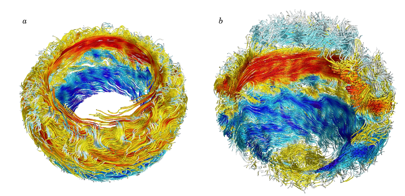
Figure 2.— Field line tracings of magnetic wreaths in case D5. $(a)$ Snapshot of two wreaths in the equatorial region at day 3880 (time t1), when the magnetic fields are strong. Lines trace the magnetic fields and color denotes the amplitude and polarity of the longitudinal field $B_{\phi}$ (red, positive; blue, negative); here the view is restricted to the equatorial region, spanning roughly $\pm 30^{\circ}$ latitude. Magnetic field threads in and out of two oppositely directed wreaths, with substantial connectivity across the equator. $(b)$ Side view spanning slightly more than one hemisphere, showing connectivity from equatorial regions to polar caps. Relic wreaths from the previous magnetic cycle are visible at the poles.

4. Patterns of Convection in Case D5

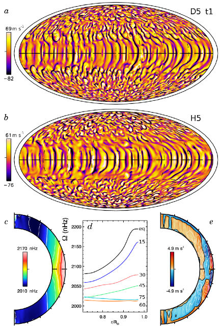
Figure 3.— Convective structures and mean flows in cases D5 and H5. $(a)$ Radial velocity $v_{r}$ in dynamo case D5 shown in global Mollweide projection at $0.95R_{\odot}$ with upflows light and downflows dark. Poles are at top and bottom and the equator is the thick dashed line, while the stellar surface at $R_{\odot}$ is indicated by the thin surrounding line. This snapshot samples day 3880 (time t1) when the magnetic fields are strong. $(b)$ Companion hydrodynamic case H5. Here stronger differential rotation shears out convective structures in the mid-latitudes. $(c)$ Profile of mean angular velocity $\Omega(r,\theta)$ for case D5, with $(d)$ radial cuts of $\Omega$ at selected latitudes. $(e)$ Meridional circulations for case D5, with magnitude and sense of circulation indicated by color (red counter-clockwise, blue clockwise) and streamlines of mass flux overlaid. The profiles shown in $(c-e)$ have been averaged over nearly 2000 days, spanning a full magnetic reversal.

The complex patterns of convection of our dynamo and hydrodynamic cases rotating at five times the solar rate are presented in Figure 3. Individual convective cells are shown in snapshots of radial velocity near the top of the simulated domain in Figures 3$a$ and $b$ for cases D5 and H5 respectively. Both cases share strong similarities in their convective patterns. Owing to the density stratification the convection is compressible and the downflows are narrow and fast, while the upflows are broader and slower.

Near the equator the prominent cells are aligned north-south and propagate in the prograde direction. The strongest flows span the entire convection zone; the weaker cells are partially truncated by the strong zonal flows of differential rotation. Nearer to the poles (above roughly $\pm 45^{\circ}$ latitude) the patterns are more isotropic. Networks of downflow lanes surround upflows and both propagate in a retrograde fashion. There is less radial shear and most of the convective cells span the full convection zone. In the polar regions, the radial velocity patterns have a somewhat cuspy appearance, with the strongest downflows appearing to favor the westward and lower-latitude side of each convective cell. This may be a consequence of the strong retrograde differential rotation in those regions.

The convective downflow structures propagate more rapidly than the differential rotation that they establish and in which they are embedded. In the equatorial band, these structures move in a prograde fashion and at high latitudes in a retrograde sense. Individual convective cells typically persist for about 10 days, though some have much longer lifetimes.

The convective structures in case D5 are quite similar to those realized in the hydrodynamic case H5 (Figure 3$b$), though there are some noticeable differences, particularly at the mid latitudes (around $\pm 30^{\circ}$). In the hydrodynamic case there is little radial flow in these regions, as the strong differential rotation shears out the convective cells. This region is equatorward of the tangent cylinder, an imaginary boundary tangent to the base of the convection zone and aligned with the rotation axis. For rotating convective shells, it has generally been found that the dynamics are different inside and outside the tangent cylinder, due to differences in connectivity and rotational constraint in these two regions (e.g., Busse 1970). The tangent cylinder in our geometry intersects with the stellar surface at roughly $\pm 42^{\circ}$ of latitude. In our compressible simulations, we generally find that the convective patterns in the equatorial regions are bounded by a conic surface rather than the tangent cylinder (Brown et al. 2008). In case H5 the strong differential rotation serves to disrupt the convection at the mid-latitudes. In contrast, in the dynamo case D5 the differential rotation is substantially weaker in both radial and latitudinal angular velocity contrasts. As is evident in Figure 3$a$, the convective cells fill in this region quite completely.

In our prior hydrodynamic simulations of convection in younger suns we reported on localized nests of convection (Brown et al. 2008), with those most prominent at the highest rotation rates. Though there is some modulation with longitude in the equatorial roll amplitudes here, this modulation is less extreme in either case D5 or H5 than in our previous rapidly rotating simulations of stellar convection (e.g., case G5 in Brown et al. 2008). This difference appears to be linked to our background stratification and feedbacks from thermal transport near the top of the domain. Here we have attempted to reduce the region of influence of the unresolved SGS heat flux $F_{u}$ which carries flux out the top of the domain (Brown et al. 2008). This thinner thermal boundary has larger gradients and a steeper profile of the background entropy gradient $\mathrm{d}\bar{S}/\mathrm{d}r$ and thus slightly higher Rayleigh numbers and radial velocities. In our broader study of rapidly rotating dynamos we have found that strongly localized active nests of convection remain possible in dynamo simulations at the most rapid rotation rates ($\Omega\gtrsim 10\>\Omega_{\odot}$).

The convection establishes a prominent solar-like differential rotation, with a fast prograde equator and slow retrograde poles. Figure 3$c$ shows the profile of mean angular velocity realized in case D5, averaged in azimuth (longitude) and time over a period of roughly 200 days centered on the time of the snapshot in Figure 3$a$. The equatorial acceleration is achieved by Reynolds stresses and convective transport that redistribute angular momentum and entropy, and build prominent gradients in latitude of angular velocity and temperature. Radial cuts of $\Omega$ indicate that strong radial shear is present throughout the lower-latitudes (Figure 3$d$). This differential rotation is solar-like in the sense that there is a monotonic decrease of $\Omega$ from the equator to the pole. Generally, the profiles here of $\Omega$ are more cylindrical than those deduced from helioseismology for the Sun, but this is to be expected for more rapidly rotating stars. This may also be influenced by our omission of a tachocline. From studies of solar convection, it is evident that the thermal structure of the tachocline with latitude influences the differential rotation profiles in the bulk of the convection zone. The main effect is to tilt the $\Omega$ contours toward a more radial alignment (Rempel 2005; Miesch et al. 2006).

The differential rotation achieved is stronger in our hydrodynamic case H5 than in our dynamo case D5. This can be quantified by measurements of the latitudinal angular velocity shear $\Delta\Omega_{\mathrm{lat}}$. Here, as in Brown et al. (2008) and Paper I, we define $\Delta\Omega_{\mathrm{lat}}$ as the shear near the surface between the equator and a high latitude, say $\pm 60^{\circ}$, with

$$\Delta\Omega_{\mathrm{lat}}=\Omega_{\mathrm{eq}}-\Omega_{60},$$ (1)

and the radial shear $\Delta\Omega_{\mathrm{r}}$ as the angular velocity shear between the surface and bottom of the convection zone near the equator with

$$\Delta\Omega_{\mathrm{r}}=\Omega_{0.97R_{\odot}}-\Omega_{0.72R_{\odot}}.$$ (2)

We further define the relative shear as $\Delta\Omega_{\mathrm{lat}}/\Omega_{\mathrm{eq}}$. In both definitions, we average the measurements of $\Delta\Omega$ in the northern and southern hemispheres, as the rotation profile is often slightly asymmetric about the equator.

These measurements are quoted for case D5 and H5 in Table 2. The angular velocity shears in case D5 can vary substantially in time as the magnetic fields wax and wane in strength. As such, here we quote measurements during one magnetic cycle with measurements averaged over the entire time interval (with label avg and date range indicated) and at periods of strongest and weakest differential rotation during this cycle (max and min respectively, at indicated times). In the hydrodynamic simulation the differential rotation shows far smaller time-variations. The global-scale magnetic fields realized in the dynamo case D5 feed back on the differential rotation and strongly diminish the amplitude of the angular velocity shears as compared with the hydrodynamic case H5. This results from both a slowing of the equatorial rotation rate and an increase in the rotation rate in the polar regions.

The angular velocity shear realized in case D5 in both latitude $\Delta\Omega_{\mathrm{lat}}$ and radius $\Delta\Omega_{r}$ is remarkably similar in amplitude to that realized in our previous dynamo simulation case D3 (Paper I) even though the basic rotation rate $\Omega_{0}$ is substantially faster. This is in striking and marked contrast to our hydrodynamic companion cases (H5 and H3) where faster rotation leads to greater angular velocity contrasts (Table 2).

Table 2Global Properties of Angular Velocity

Case	$\Delta\Omega_{\mathrm{lat}}$	$\Delta\Omega_{\mathrm{r}}$	$\Delta\Omega_{\mathrm{lat}}/\Omega_{\mathrm{eq}}$	Epoch
D5${}^{\text{{avg}}}$	1.14	0.71	0.083	3500–5500
D5${}^{\text{{min}}}$	0.91	0.39	0.067	3702
D5${}^{\text{{max}}}$	1.43	0.98	0.102	4060
H5	2.77	1.31	0.192	-
D3	1.18	0.71	0.137	2010-6980
H3	2.22	0.94	0.246	-

Note. — Angular velocity shear in units of $\mu\mathrm{rad}\>\mathrm{s}^{-1}$, with $\Delta\Omega_{\mathrm{lat}}$ measured near the surface ($0.97R_{\odot}$) and $\Delta\Omega_{\mathrm{r}}$ measured across the full shell at the equator. The relative latitudinal shear $\Delta\Omega_{\mathrm{lat}}/\Omega_{\mathrm{eq}}$ is also shown. For the dynamo cases, these measurements are taken over the indicated range of days. In oscillating dynamo case D5, these measurements are averaged over a long epoch (avg), and are also taken at two short intervals in time when the differential rotation is particularly strong (max) and when magnetic fields have suppressed this flow (min). The hydrodynamic case H5 is averaged for roughly 300 days and shows no systematic variation on longer timescales. Measurements for cases D3 and H3 rotating at $3\>\Omega_{\odot}$ are quoted from Paper I.

The differential rotation profiles realized in these rapidly rotating simulations are substantially in thermal wind balance (e.g., Brun & Toomre 2002; Miesch et al. 2006; Brown et al. 2008), though large departures do arise near the inner and outer boundaries where Reynolds stresses and boundary conditions play a dominant role. Maxwell stresses are significant in the cores of the magnetic wreaths realized in dynamo case D5, but these play relatively little role in the global transport of angular momentum. During a reversal, these Maxwell stresses do however transport angular momentum toward the poles, giving rise to bands of quickly flowing fluid that share some similarities with the torsional oscillations observed during the solar cycle. This behavior will be explored in Section 9.

The meridional circulation patterns for case D5 are shown in Figure 3$e$. There appear to be three major cells of circulation in each hemisphere, with several cells in both radius and latitude. Strong rotational constraint in regions outside the tangent cylinder likely leads to the significantly cylindrical nature of these slow flows. Some flows along the inner and outer boundaries cross the tangent cylinder and serve to weakly couple the polar regions to the equatorial regions. These meridional circulations are very similar to the circulations found in case H5. In both simulations, the meridional circulations are weaker, slower and more multi-celled than those realized in simulations rotating at the slower rotation rates (Brown et al. 2008, 2010). The slower flows and multi-cellular nature of these meridional circulations may have strong implications for flux transport dynamos (e.g., Bonanno et al. 2006; Jouve & Brun 2007; Jouve et al. 2010).

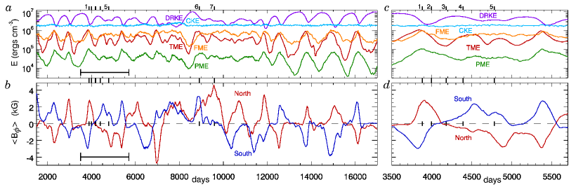
Figure 4.— Complex time evolution in case D5 with flips in polarity of magnetic wreaths. $(a)$ Volume-averaged energy densities for kinetic energy of convection (CKE), differential rotation (DRKE) and for magnetic energy in fluctuating fields (FME), in mean toroidal fields (TME) and in mean poloidal fields (PME) as labeled. Oscillations on roughly 500-1000 day periods are visible in the magnetic energies and in DRKE, though CKE stays nearly constant. $(b)$ Mean toroidal field $\langle B_{\phi}\rangle$ averaged over entire northern and southern hemispheres (labeled) at mid-convection zone ($0.85R_{\odot}$). Early in the simulation, opposite polarities dominate each hemisphere. Several reversals occur, along with several extreme excursions which do not flip the polarity of the global-scale field. During the interval from roughly day 7700 to 10200, the dynamo falls into peculiar single polarity states, with one polarity dominating both hemispheres. Bracketed interval from day 3500 to 5700 spans one full polarity reversal; $(c)$ expanded view of volume-averaged energy densities during this period, and $(d)$ the mean toroidal field with same vertical axis scales as in $(a,b)$. Thick labeled tick marks above $a,c$ indicate time samples used in later images.

5. Oscillations in Energies and Changes of Polarity

A striking feature of the convective dynamo case D5 is its time dependence. This time-varying behavior is readily visible as oscillations of the volume-averaged kinetic and magnetic energy densities, as shown in Figure 4$a$ at a time long after the dynamo has saturated and reached equilibration.

Here the kinetic energy of differential rotation (DRKE) undergoes factor of five changes on periods of 500-1000 days. As DRKE decreases the magnetic energies increase. Moving in concert are the mean toroidal (TME) and mean poloidal (PME) magnetic energies. The mean poloidal fields appear to lag slightly behind the mean toroidal fields as they both change in strength. The fluctuating magnetic energy (FME) tracks the largest rises in the mean fields but decouples during many of the deepest dips. In contrast, the variations in convective kinetic energy (CKE) shows little organized behavior in time, and appears to change substantially only when the differential rotation is highly suppressed during the period from day 7500 to day 8300. The energy contained in the meridional circulations (MCKE) is weaker and not shown. Though it varies somewhat in time, there is not a clear relation to the changes in magnetic energies. These energies are defined as

$$\mathrm{CKE} = \frac{1}{2}\bar{\rho}\Big{[}\left(v_{r}-\langle v_{r}\rangle\right)^{2}+\left(v_{\theta}-\langle v_{\theta}\rangle\right)^{2}+$$ (3)

$$\qquad\left(v_{\phi}-\langle v_{\phi}\rangle\right)^{2}\Big{]},$$

$$\mathrm{DRKE} = \frac{1}{2}\bar{\rho}\langle v_{\phi}\rangle^{2},$$ (4)

$$\mathrm{MCKE} = \frac{1}{2}\bar{\rho}\Big{(}\langle v_{r}\rangle^{2}+\langle v_{\theta}\rangle^{2}\Big{)},$$ (5)

$$\mathrm{FME} = \frac{1}{8\pi}\Big{[}\left(B_{r}-\langle B_{r}\rangle\right)^{2}+\left(B_{\theta}-\langle B_{\theta}\rangle\right)^{2}+$$ (6)

$$\qquad\left(B_{\phi}-\langle B_{\phi}\rangle\right)^{2}\Big{]},$$

$$\mathrm{TME} = \frac{1}{8\pi}\langle B_{\phi}\rangle^{2},$$ (7)

$$\mathrm{PME} = \frac{1}{8\pi}\Big{(}\langle B_{r}\rangle^{2}+\langle B_{\theta}\rangle^{2}\Big{)}.$$ (8)

where angle brackets will consistently denote an average in longitude.

Magnetic energies in case D5 can rise to be a substantial fraction of the kinetic energies. Averaged over the nearly 16000 days (about 44 years) shown here, the magnetic energies are about 17% of the kinetic energies. During individual oscillations the magnetic energies can range from a few percent of the kinetic energies to levels as high as 50%. The kinetic energy is largely in the fluctuating convection and differential rotation, with CKE fairly constant and ranging from 15-60% of the total kinetic energy as DRKE grows and subsides, itself contributing between 40 to 85% of the kinetic energy. The magnetic energies are largely split between the mean toroidal fields and the fluctuating fields, with TME containing about 35% of the magnetic energy on average, FME containing about 61% and PME containing 4%. The roles of these energy reservoirs change somewhat through each oscillation. At any one time, between 10 and 60% of the magnetic energy is in TME while FME contains between 30 and 85% of the total. Meanwhile, PME can comprise as little as 1% or as much as 10% of the total. Generally, PME is about 12% of TME, but because PME lags the changes in TME slightly, there are periods of time when PME is almost 40% of TME.

These results are in contrast to our previous simulations of the solar dynamo, where the mean fields contained only a small fraction of the magnetic energy (e.g., Brun et al. 2004, where TME and PME comprise about 2% of the total). Simulations of dynamo action in fully-convective M-stars do however show high levels of magnetic energy in the mean fields (Browning 2008). In those simulations the fluctuating fields still contain much of the magnetic energy, but the mean toroidal fields possess about 18% of the total throughout most of the stellar interior. Simulations of dynamo action in the convecting cores of A-type stars (Brun et al. 2005) achieve similar results though when fossil fields are included, those dynamos can reach states with super-equipartition magnetic field strengths and strong mean fields (Featherstone et al. 2009). In our rapidly rotating suns, the mean fields comprise a significant portion of the magnetic energy in the convection zone and are as important as the fluctuating fields. In the wreath-building dynamo case D3 rotating at three times the current solar rate (Paper I) we found that the mean toroidal fields contained roughly 43% of the magnetic energy and the mean poloidal fields contained about 4%, with the rest in the fluctuating fields.

The global-scale magnetic fields can reverse their polarities during some of the oscillations in magnetic energies. This is evident in Figure 4$b$ showing averages at mid-convection zone of the longitudinal magnetic field $\langle B_{\phi}\rangle$ over the northern and southern hemispheres. Reversals in field polarity occur periodically, with typical time scales of roughly 1500 days. These reversals appear to happen shortly after peak magnetic energies are achieved, but do not occur every time magnetic energies undergo a full oscillation. Rather, for each successful polarity reversal it appears that several failed reversals occur where the magnetic energies drop and the average fields decline in strength, only to return with the same polarity a few hundred days later.

We focus in the following discussion on one such reversal, shown in closeup in Figures 4$c,d$ and spanning the interval of time between days 3500 and 5700. Two reversals occur during this interval, with the global polarities flipping into a new state at roughly day 4100 and then changing back again at about day 5500. Detailed measurements of kinetic and magnetic energies during this interval are shown in Table 3.

Table 3Kinetic and Magnetic Energies

Case	CKE	DRKE	MCKE	FME	TME	PME
D5${}^{\text{{avg}}}$	$1.85$	$4.46$	$0.006$	$0.55$	$0.43$	$0.048$
D5${}^{\text{{min}}}$	$1.70$	$2.85$	$0.005$	$0.50$	$0.25$	$0.062$
D5${}^{\text{{max}}}$	$1.85$	$7.52$	$0.007$	$0.39$	$0.65$	$0.042$
H5	$2.27$	$34.3\phantom{0}\phantom{0}$	$0.008$	-	-	-

Note. — Volume-averaged energy densities relative to the rotating coordinate system. Kinetic energies are shown for convection (CKE), differential rotation (DRKE) and meridional circulations (MCKE). Magnetic energies are shown for fluctuating magnetic fields (FME), mean toroidal fields (TME) and mean poloidal fields (PME). All energy densities are reported in units of $10^{6}\mathrm{erg}\>\mathrm{cm}^{-3}$. In time-varying case D5, these energies are averaged over the intervals defined in Table 2, while in case H5 an arbitrary 1000 day interval was chosen.

6. Global-Scale Magnetic Reversals

6.1. Toroidal Field Reversals

The nature of the global-scale magnetic fields during the reversal spanning days 3500–5700 are presented in detail in Figure 5. Several samples of longitudinal magnetic field $B_{\phi}$ are shown at mid-convection zone spanning this time period. The timing of these samples is indicated in Figure 4 by numeric labels and likewise in Figure 5$a$ which shows azimuthally-averaged $\langle B_{\phi}\rangle$ at this depth in a time-latitude map that spans the reversal. The evolution of the mean toroidal field near the base of the convection zone is discussed in Section 8 and Figure 10$a$.

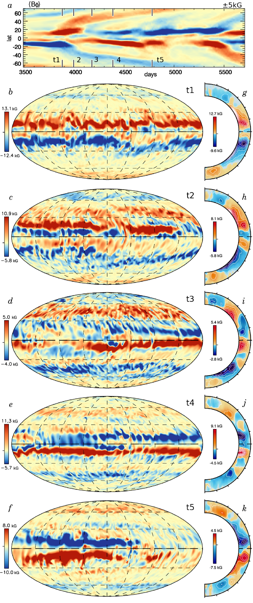
Figure 5.— Evolution of longitudinal field $B_{\phi}$ during a polarity reversal in case D5. $(a)$ Time-latitude plot of $\langle B_{\phi}\rangle$ at mid-convection zone, with sampling times indicated. $(b-f)$ Snapshots of $B_{\phi}$ in Mollweide projection at mid-convection zone ($0.85R_{\odot}$) at times indicated. Between reversals the field is dominated by the mean component, but during reversals substantial fluctuations develop. $(g-k)$ Accompanying samples of azimuthally-averaged $\langle B_{\phi}\rangle$, showing structure of mean fields with radius and latitude at same instants in time. The companion poloidal fields are shown in Figure 7.

Before a reversal, the magnetic wreaths of case D5 are very similar in appearance to the wreaths realized in our persistent wreath-building dynamo case D3 (Paper I). They are dominated by the azimuthally-averaged component of $B_{\phi}$, while also showing small-scale variations where convective plumes distort the fields (Figure 5$b$). At mid-convection zone, typical longitudinal field strengths are of order $\pm 13$ kG, while peak field strengths there can reach $\pm 40$ kG. Meanwhile $\langle B_{\phi}\rangle$ is fairly antisymmetric between the northern and southern hemispheres (Figure 5$g$). Shortly before a reversal, the magnetic wreaths strengthen in amplitude and become more antisymmetric about the equator.

They reach their peak values just before the polarity change at roughly day 4000 but then quickly begin to unravel, gaining significant structure on smaller scales (Figure 5$c$). At the same time, prominent magnetic structures detach from the higher-latitude edges and begin migrating toward the polar regions. Meanwhile, $\langle B_{\phi}\rangle$ loses its antisymmetry between the two hemispheres, with $\langle B_{\phi}\rangle$ in one hemisphere typically remaining stronger and more concentrated than in the other (Figure 5$h$). The stronger hemisphere (here the northern) retains its polarity for about 100 days as the fields in the other hemisphere (here southern) weaken and reverse in polarity. At this point the new wreaths of the next cycle, with opposite polarity, are already faintly visible at the equator.

Within another 100 days these new wreaths grow in strength and become comparable with the structures they replace, which are still visible at higher latitudes (Figures 5$d,i$). The mean $\langle B_{\phi}\rangle$ begins to contribute significantly to the overall structure of the new wreaths, and soon the polarity reversal is completed. In the interval immediately after the reversal, small-scale fluctuations still contribute significantly to the overall structure of the wreaths, and $B_{\phi}$ has a complicated structure at mid-convection zone. At this time, the peak magnetic field strengths are somewhat lower, at about $\pm 20$ kG. As $\langle B_{\phi}\rangle$ becomes stronger, the wreaths return to an antisymmetric state, with similar amplitudes and structure in both the northern and southern hemispheres (Figures 5$e,j$). They look much as they did before the reversal, though now with opposite polarities.

The wreaths from the previous cycle appear to move through the lower convection zone and toward higher latitudes. This can be seen variously in the time-latitude map at mid-convection zone (Figure 5$a$), in the Mollweide snapshots (Figures 5$b$–$f$), as well as in the samples of $\langle B_{\phi}\rangle$ (Figures 5$g$–$k$). This poleward migration appears to be partially due to a dynamo wave (Section 8) and partially due to hoop stresses within the magnetic wreaths and an associated poleward-slip instability (e.g., Spruit & van Ballegooijen 1982; Moreno-Insertis et al. 1992, and our Section 9). Even at late times some signatures of the previous wreaths persist in the polar regions, and are still visible in Figures 5$e,j$ at day 4390. They are much weaker in amplitude than the wreaths at the equator, but they persist until the wreaths from the next cycle move poleward and replace them. As they approach the polar regions, the old wreaths dissipate on both large and small scales, for the vortical polar convection shreds them apart and ohmic diffusion reconnects them with the relic wreaths of the previous cycle. The $\Omega$-effect also contributes both to the low-latitude generation of the wreaths and their high-latitude decay (Section 8).

Though reversals occur on average once every 1500 days, substantial variations can occur on shorter time scales. Here at mid-cycle the wreaths become concentrated in smaller longitudinal intervals of the equatorial region (as in Figures 5$f,k$ at day 4780). At other times the mean longitudinal fields become quite asymmetric, with one hemisphere strong and one weak (i.e., during days 4900–5200) before regaining their antisymmetric nature shortly prior to the next reversal.

6.2. Connections Across the Equator

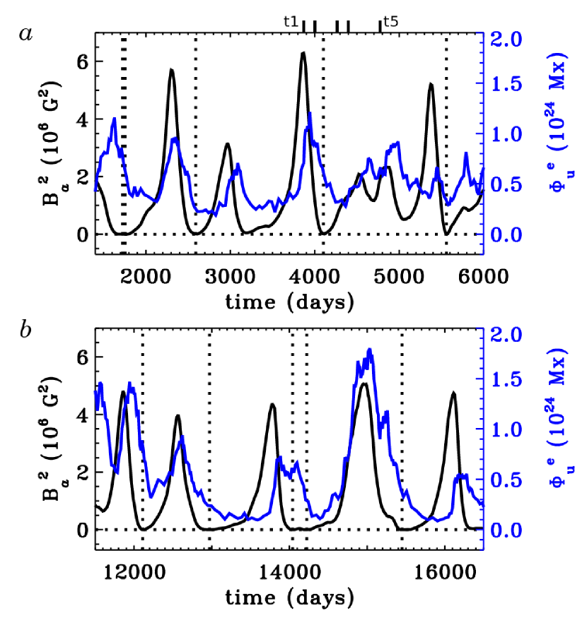
Figure 6.— The squared magnitude of the antisymmetric, low-latitude toroidal field component $B_{a}^{2}(t)$ (black lines, left axes) and the unsigned flux across the equator $\Phi_{u}^{e}(t)$ (blue lines, right axes) as a function of time for two selected intervals when the wreaths of opposite polarity occupy each hemisphere: ($a$) $t=$ 1400–6000 (days), and ($b$) 11,500–16,500 (days). Vertical dotted lines indicate polarity reversals, defined as where $B_{a}(t)$ changes sign. Labeled tick marks at top indicate times t1–t5. Generally, the unsigned flux $\Phi_{u}^{e}(t)$ is larger when $B_{a}^{2}$ is decreasing. During the interval 6000–11,500 days (not shown) the dynamo is in an unusual state in which wreaths in both hemispheres have the same magnetic polarity.

The oppositely-directed wreaths are not isolated entities. Rather, they interact through complex magnetic linkages across the equator that contribute to their erosion and subsequent reversal.

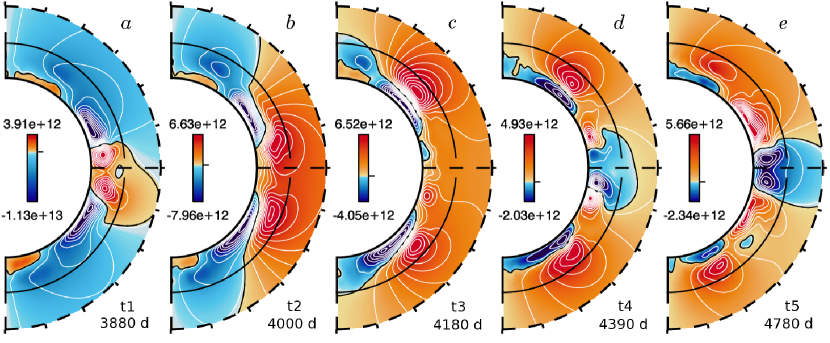
Figure 7.— Evolution of poloidal field during a polarity reversal in case D5. Shown are the vector potential of the mean poloidal field $\langle A_{\phi}\rangle$ in case D5 at times t1–t5 (with corresponding days noted). Colors denote amplitude and polarity (red clockwise; blue, counterclockwise); units are G cm. The stellar surface is indicated with a solid line, and the poloidal field is extended with a potential field extrapolation to 1.3 R_⊙ (dashed surface). Reversals of poloidal field appear to begin in the equatorial region $(a)$ and spread through the upper convection zone $(b,c)$ before new reversed polarity appears at the equator $(d,e)$. The toroidal fields have largely reversed in the equatorial region by time t3 (see Figure 5$d,i$).

The magnetic linkages between hemispheres can be quantified by the net unsigned magnetic flux through the equatorial plane:

$$\Phi_{u}^{e}(t)=\int_{r_{1}}^{r_{2}}\int_{0}^{2\pi}\left|B_{\theta}(r,\theta_{\mathrm{eq}},\phi)\right|r\sin\theta_{e}\mathrm{d}r\mathrm{d}\phi,$$ (9)

where $\theta_{\mathrm{eq}}=\pi/2$ and where $r_{1}=r_{\mathrm{bot}}$ and $r_{2}=r_{\mathrm{top}}$. In order to relate this quantity to polarity reversals of the toroidal wreaths we define the antisymmetric component of the mean, low-latitude toroidal field as follows

$$B_{a}(t)=V^{-1}\int_{r_{1}}^{r_{2}}\int_{\theta_{\mathrm{eq}}-\delta}^{\theta_{\mathrm{eq}}+\delta}\int_{0}^{2\pi}h(\theta)B_{\phi}(r,\theta,\phi)r^{2}\sin\theta\mathrm{d}r\mathrm{d}\theta\mathrm{d}\phi\>,$$ (10)

where

$$V=\int_{r_{1}}^{r_{2}}\int_{\theta_{\mathrm{eq}}-\delta}^{\theta_{\mathrm{eq}}+\delta}\int_{0}^{2\pi}r^{2}\sin\theta\mathrm{d}r\mathrm{d}\theta\mathrm{d}\phi=\frac{4\pi}{3}\left(r_{2}^{3}-r_{1}^{3}\right)\cos(\theta_{e}-\delta)\>.$$ (11)

Here $h(\theta)$ is a step function with $h(\theta)=1$ for $\theta<\theta_{e}$, $h(\theta)=-1$ for $\theta>\theta_{e}$, and $h(\theta_{e})=0$. We set $\delta=2\pi/9$ (40^∘) in order to focus on the low-latitude wreaths and then plot the squared amplitude of this quantity.

Figure 6 shows $\Phi_{u}^{e}(t)$ and $B_{a}^{2}(t)$ versus time for the two intervals in the simulation when cyclic magnetic activity is most apparent. The interval spanning days 6000–11,500 is not shown as the dynamo had fallen into a peculiar single polarity state and had temporarily stopped showing cyclic behavior; we defer discussion of that interval until Section 10. Labeled tick marks at the top of Figure 6$a$ indicate times t1–t5 shown previously during the reversal in Figure 5 (days 3880 to 4780).

Examining this interval, we see that the squared amplitude of antisymmetric mean field $B_{a}^{2}$ attains a peak value near time t1 shortly before the reversal and then drops to a minimum as the global-scale fields reverse in polarity (reversal denoted by vertical dotted line at roughly day 4100). Some of this decrease is due to the poleward propagation of the magnetic wreaths. In Figure 5$a$ we see that at mid-convection zone, the wreaths of the preceding cycle have largely left the region $\pm 40^{\circ}$ latitude by day 4100, leaving the wreaths of new polarity at the equator. $B_{a}^{2}$ then slowly grows in amplitude before again attaining a sharp maximum and reversing in sense (near day 5500). The unsigned flux through the equator $\Phi_{u}^{e}$ lags somewhat behind the mean fields, peaking near time t2 and dropping to a minimum at approximately day 4200. The unsigned flux, measuring cross-equatorial connectivity, does not drop to zero during any of the intervals studied here.

Clearly, the decay and subsequent reversal of antisymmetric toroidal wreaths is strongly correlated with enhanced magnetic linkages across the equator. To quantify this relationship, we define the rising and decaying phases of a cycle as those intervals when the temporal derivative of $B_{a}^{2}(t)$ is positive and negative respectively. Then we proceed to compute the average value of $\Phi_{u}^{e}(t)$ in declining phases relative to rising phases. For the two time intervals shown in Figure 6, this ratio is ($a$) 2.7 and ($b$) 1.9. Over the entire extended simulation interval (1400–18,252 days) the ratio of unsigned flux in declining versus rising phases is 1.7. Thus, there is significantly more unsigned flux across the equator when the wreaths are declining in amplitude or undergoing a reversal.

6.3. Poloidal Field Reversals

The evolution of the mean poloidal field can be followed by examining how its vector potential $\langle A_{\phi}\rangle$ evolves in time, where

$$\langle\boldsymbol{B}_{\mathrm{pol}}\rangle=\langle B_{r}\rangle\boldsymbol{\hat{r}}+\langle B_{\theta}\rangle\boldsymbol{\hat{\theta}}=\nabla\times\langle A_{\phi}\boldsymbol{\hat{\phi}}\rangle,$$ (12)

with unit vectors denoted by hats and angle brackets again denoting an average in longitude. The vector potential of the mean poloidal magnetic field $\langle A_{\phi}\rangle$ is shown in snapshots at times t1–t5 during the reversal in Figure 7, with color denoting polarity and poloidal field lines represented by the overlying contours. A potential field extrapolation has been used to follow the poloidal field above the surface out to a distance of $1.3\>R_{\odot}$.

When the magnetic fields are strong (i.e., at time t1, Fig. 7$a$) the poloidal field is dominated by odd-$\ell$ components, with significant dipolar and octupolar contributions. The polar regions have the same polarity (here negative), while the equatorial region has opposite polarity (here positive). The transition between poloidal polarities occurs in the cores of the magnetic wreaths, where $\langle B_{\phi}\rangle$ is strong (near $\pm 15^{\circ}$ latitude).

During the course of a reversal, $\langle A_{\phi}\rangle$ grows in amplitude in the equatorial region. The equatorial polarity expands to fill the upper convection zone (times t2–t3, Figs. 7$b,c$) while in the lower convection zone the dominant polar polarity begins to disappear. At the same times, toroidal field of the new opposite polarity is appearing in this equatorial region (Fig. 5$c,d,h,i$). Indeed, by time t3 the wreaths of the new cycle are well established and the wreaths of the previous cycles are propagating towards the polar regions.

The poloidal field of equatorial polarity from the previous cycle (positive in the reversal shown in Figure 7) replaces the poloidal field at the poles, while in the equatorial region oppositely directed poloidal field begins to appear at the equator (here negative and visible at time t4). This occurs as the new wreaths of toroidal field grow in strength and attain a high degree of axial symmetry with $\langle B_{\phi}\rangle$ contributing substantially to the structure of the toroidal field. At this point the reversal is complete, though flux continues to cancel in the lower convection zone, leading to the final reversed state shown in Figure 7$e$.

7. Evolution of Large-Scale Moments

The turbulent convection in case D5 gives rise both to small-scale, rapidly evolving magnetism, and to slowly evolving ordered fields on larger scales. One manifestation of the latter is the generation of wreaths of toroidal field, whose strength and temporal evolution we have already described. Another is the presence of remarkably strong dipole, quadrupole and octupolar components of the poloidal field. These low-order moments of the field do not dominate the magnetic energy – indeed, near the top of the simulation domain, modes with spherical harmonic degree $\ell=1$–$3$ typically contain no more energy than modes with $\ell$ up to $20$. But these low-order modes hold particular significance both theoretically and observationally: in the Sun, for instance, the evolution of the global dipole moment is tightly linked to the sunspot cycle, with the phasing relationship between the two (the sign of the surface dipole reverses near solar maximum) serving as an important constraint on models of the solar dynamo (e.g., Wang & Sheeley 1991; Charbonneau & MacGregor 1997).

More generally, the low-order modes of the magnetic field are important both as diagnostics of global-scale dynamo action and as mediators that regulate the interaction of a star with its surroundings. Because higher-order multipoles fall off quickly with radius, the dipole mode dominates the magnetic energy distribution at large distances from the stellar surface, and so may contribute most to the magnetic “lever arm” that determines how rapidly a star’s rotation is braked (e.g., Weber & Davis 1967; Matt & Pudritz 2008). Low-order multipoles also regulate the interaction of pre-main-sequence stars with their surrounding accretion disks (e.g., Shu et al. 1994), with broad implications for the truncation of those disks and the formation of protoplanetesimals. Such considerations warrant a careful consideration of the multipolar structure and evolution in case D5.

7.1. The Wandering Dipole

The lowest-order moment is the dipole, the components of which sum vectorally to give a time-evolving quantity with both magnitude and direction. Figure 8 illustrates the the evolution of the dipole vector over the course of one polarity reversal.

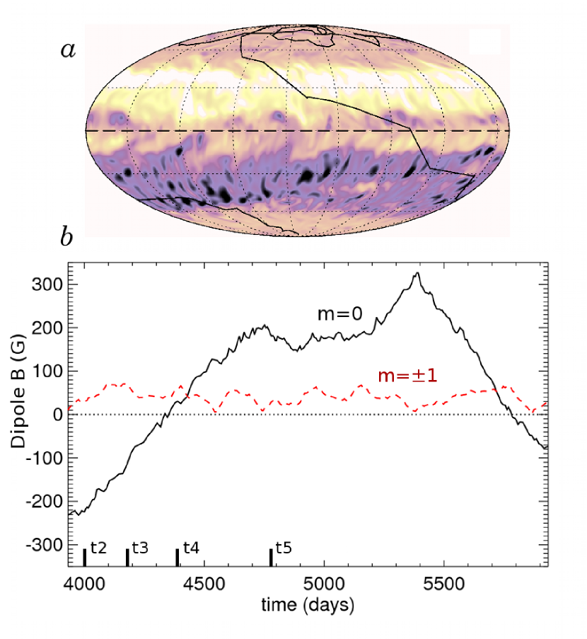
Figure 8.— Evolution of dipole field in the lower-convection zone during one magnetic reversal, with times t2–t5 noted. ($a$) Location of the maximum in the dipole ($\ell=1$) magnetic field (the positive magnetic pole) as measured at $0.73R_{\odot}$ is traced by the solid black line, with $B_{\phi}$ at time t2 and at the same depth shown in background. ($b$) Relative strengths of the axisymmetric ($m=0$) and non-axisymmetric ($m=\pm 1$, added in quadrature) terms of the dipole. The axisymmetric dipole smoothly evolves from negative to positive during the reversal while the non-axisymmetric fields fluctuate continuously and show little sign of the global-scale polarity reversal. A second reversal occurs after day 5500.

The location of the positive magnetic pole in the lower-convection zone is traced in Figure 8$a$ over a period of roughly 2000 days, displayed on a surface near the base of the convection zone. This track was calculated by filtering the radial field $B_{r}$ in spectral space (retaining only $\ell=1$ modes), transforming back to physical space, and tracking the longitude and latitude of the maximum in the resulting field distribution. In Figure 8$a$, the latitude of the pole generally stays close to the geographic north or south pole, except during reversals of the overall polarity. These reversals are the only time during the interval studied here that the pole “tips” to latitudes of less then about $\pm 45$ degrees. The longitudinal position of the pole fluctuates more erratically, with no orderly sense of propagation. In examining both the longitude and latitude of the $\ell=1$ maxima and thus including contributions from modes with $m=\pm 1$ as well as $m=0$, we are effectively probing the evolution of the “equatorial dipole” (e.g., Wang & Sheeley 1991) in addition to the “axial dipole” associated with the $m=0$ modes. The strength of this equatorial dipole, and the tipping of the magnetic poles away from the geographic poles, are indications of the non-axisymmetric contributions to the magnetism.

A quantitative assessment of non-axisymmetry is provided by Figure 8$b$, which shows the magnitude of the $m=0$ component of the dipole and the amplitude of the $m=\pm 1$ dipole components added in quadrature during a roughly 2000-day interval around this reversal (with second reversal occuring after day 5500). As the mean toroidal field in the wreathes reverses polarity (Fig. 5), the axial dipole diminishes in strength and changes sign, while the non-axisymmetric pieces fluctuate erratically and do not seem to sense the global-scale reversal.

The erratic evolution of the non-axisymmetric field components, as compared to the relatively smooth evolution of the $m=0$ field, suggests that the dominant processes generating non-axisymmetric fields are somewhat different from those responsible for axisymmetric fields. Both the “wandering of the poles” in longitude (Fig. 8$a$) and the fluctuating $m=\pm 1$ field amplitudes (Fig. 8$b$) would be expected if non-axisymmetric field generation were associated mainly with small-scale magnetic features, that add with random phases to yield a small (but non-zero) contribution to the dipole. The longitude of the pole might then be expected to undergo a random walk on timescales comparable to the convective eddy turnover time. This is consistent with what we observe in case D5.

The smooth latitudinal migration of the magnetic pole, on the other hand, suggests that the global-scale field reversals that occur in case D5 rely on more than just the random agglomeration of uncorrelated small-scale magnetic elements. Thus the global-scale axisymmetric $m=0$ fields evolve in a fashion distinct from the non-axisymmetric components. We note that when we try to assess the evolution of the dipole field in the fashion shown here at the mid-convection zone or near the stellar surface, we find that the dipole there is much more variable in time. At these higher radial levels the dipole shows several reversals which do not correspond to the global-scale reversals of toroidal and poloidal polarity. Instead in the upper convection zone, the higher-order modes of the poloidal field more accurately track the reversals occurring throughout the convection zone. We consider these in Section 7.2.

7.2. Axisymmetric Dipole, Quadrupole and Octupole

The temporal evolution of the axisymmetric dipole, quadrupole, and octupole moments of the poloidal field can be assessed by measuring the amplitudes of the $m=0$ components of the radial magnetic field $B_{r}$. These amplitudes are defined here as

$$\mathcal{D} = \sqrt{\frac{3}{4\pi}}\int{B_{r}\cos{\theta}\sin{\theta}\mathrm{d}\theta\mathrm{d}\phi}$$ (13)

$$\mathcal{Q} = \frac{1}{2}\sqrt{\frac{5}{4\pi}}\int{B_{r}(3\cos^{2}{\theta}-1)\sin{\theta}\mathrm{d}\theta\mathrm{d}\phi}$$ (14)

$$\mathcal{O} = \frac{1}{2}\sqrt{\frac{7}{4\pi}}\int{B_{r}(5\cos^{3}{\theta}-3\cos{\theta})\sin{\theta}\mathrm{d}\theta\mathrm{d}\phi}$$ (15)

where the integral solid angle is at fixed radius (e.g., Arfken & Weber 1995). The quantity $\mathcal{D}$ is often termed the “axial dipole” in solar physics (e.g., Wang & Sheeley 1991).

The amplitudes $\mathcal{D}$, $\mathcal{Q}$, and $\mathcal{O}$ (the $\ell=1,2,3$ components of the $m=0$ field) are shown over an extended interval of about 13,000 days in Figure 9. Here, the measurements are integrated over two spherical surfaces, with one near the top of the convection zone (Fig. 9$a$, at $0.97R_{\odot}$) and another near the base of the convection zone (Fig. 9$b$, at $0.73R_{\odot}$). The octupole moment is generally the strongest, particularly when the oppositely-directed wreathes are most prominent, but the dipole and quadrupole moments are also significant. The typical amplitude of these multipoles is comparable to that realized in simulations of solar convection with large-scale fields (Browning et al. 2006), and stronger than in simulations of small-scale dynamo action by solar convection with potential field lower boundary conditions (Brun et al. 2004). They are also substantially stronger than the surface dipole moment observed on the Sun (e.g., Wang & Sheeley 1991; Schrijver & De Rosa 2003). Peak pointwise values of the 3D radial field $B_{r}$ typically exceed 1 kG.

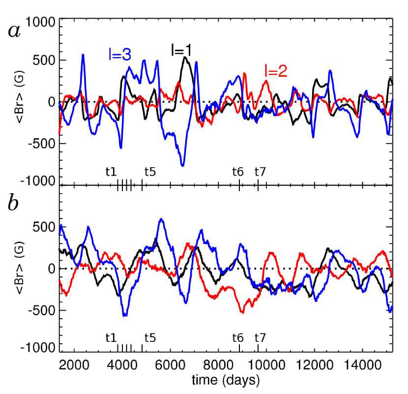
Figure 9.— Temporal evolution of low-degree moments of the poloidal field. Shown are the axisymmetric ($m=0$) components of the dipole, quadrupole and octupole moments ($\mathcal{D}$, $\mathcal{Q}$, and $\mathcal{O}$, with $\ell=1,2,3$ respectively) of the radial magnetic field $B_{r}$ at two depths: ($a$) near the surface at $0.97\>R_{\odot}$ and ($b$) near the base of the convection zone at $0.73\>R_{\odot}$. At depth, the octupole moment consistently lags the dipole. During the interval roughly spanning days 7300–10200 the dynamo enters an unusual symmetric polarity state and the quadrupole state becomes strong and does not reverse. After this period, normal cyclic behavior resumes.

Interpreting the evolution of the axisymmetric poloidal field is made challenging by the nontrivial depth dependence that the various moments exhibit. Near the top of the convection zone, the dipole moment $\mathcal{D}$ changes sign about twenty times over the 13000 days sampled, although some excursions to one polarity or the other are short-lived (Fig. 9$a$). These polarity reversals are separated by fairly irregular intervals of 300 to 1500 days. The sign of the axisymmetric quadrupole component $\mathcal{Q}$ flips somewhat more frequently, undergoing a few reversals that are not reflected in the dipole moment. Generally the dipole and quadrupole track each other well in time, with no consistent lag between the two moments. The octupole reverses less frequently than either the dipole or quadrupole, and when it does reverse it generally lags them slightly in time.

In the lower convection zone (Fig. 9$b$), the moments evolve relatively slowly, with fewer reversals separated by significantly longer intervals of about 1500 days. The octupole moment consistently lags a few hundred days behind the dipole. The longer evolution times in the lower convection zone could plausibly reflect the longer Alfvén times deeper down or the longer magnetic diffusion time – for our choice of SGS magnetic diffusivity $\eta$, scaling with $\bar{\rho}^{-1/2}$, both timescales vary in roughly the same fashion with depth. Convective time scales also decrease toward the bottom of the convection zone and the ratio of magnetic to kinetic energy increases. Thus, the more stable mean fields may reflect less buffeting by convective motions.

The temporal variations in these low-degree moments are linked to the reversals of toroidal field, but the relationship between the different field components is complex. Near the surface, the octupole tracks the deep-seated toroidal fields fairly well, but the dipole and quadrupole moments exhibit flips which do not correspond to global-scale reversals. In the lower convection zone, it appears that the dipolar reversal precedes the octupolar reversals. Typically the reversal of the dipole occurs shortly after the octupole is near its peak amplitude (e.g., at about time t4). The octupole then generally reverses when the dipolar moment is near a maximum in amplitude (e.g., about time t5). Most of the reversals in dipole and octupole polarity deep in the lower convection zone correspond to a flip in the sign of the predominant toroidal field in each hemisphere, but typically occur only after the wreaths have reversed their polarities in the near equatorial region (this occurs by time t3 in our example reversal).

When the dipole and octupole are strong, we generally see wreaths that are antisymmetric about the equator. When the quadrupole becomes stronger (e.g., during the interval from roughly 7000–10000 days) the dynamo typically exhibits toroidal fields that are symmetric about the equator. This indicates that the global-scale toroidal field is likely being produced by the stretching of global-scale poloidal field by the shear of differential rotation.

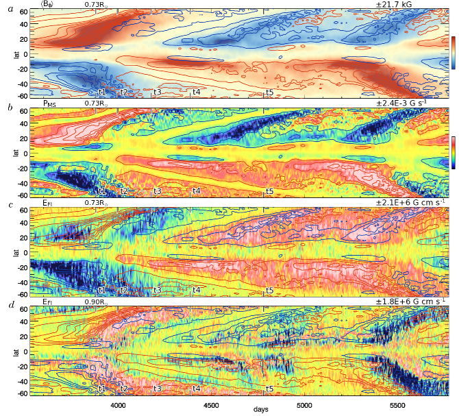
Figure 10.— Temporal and latitudinal variation of magnetic fields and the effects that generate them. ($a$) Longitudinally-averaged toroidal field $\langle B_{\phi}\rangle$ near the base of the convection zone ($0.73R_{\odot}$), as image and contour plot in latitude and time. ($b$) Production of toroidal fields by mean shear $P_{\mathrm{MS}}$. ($c$) Longitude-averaged turbulent electromotive force $E_{\mathrm{FI}}$ which generates poloidal vector potential $\langle A_{\phi}\rangle$. ($d$) Same emf $E_{\mathrm{FI}}$ shown in the upper convection zone ($0.90R_{\odot}$). Contours of $P_{\mathrm{MS}}$ at $0.73R_{\odot}$ are overplotted in all panels for reference (red positive, blue negative). These contours have been smoothed with a 35-day moving time average.

8. A Nonlinear Dynamo Wave

The latitudinal propagation and orderly reversal of large-scale magnetic fields realized in case D5 constitute a striking finding of these simulations. Here we examine how field propagation and reversal might arise, by examining the spatial and temporal dependence of some of the mechanisms that act to strengthen or weaken fields.

Spatial propagation and field reversals may be expected whenever the processes that amplify or reduce a magnetic field – i.e., source terms in the induction equation – are out of phase spatially or temporally with the field itself. In mean-field solar dynamo models, such spatial propagation can arise through the combined operation of the $\alpha$-effect and $\Omega$-effect in the form of a “dynamo wave” (e.g., Stix 1976; Yoshimura 1976). In mean-field solar dynamo models that employ a spatial separation between poloidal and toroidal source regions, flux transport by the meridional circulation, turbulent pumping, or turbulent diffusion can produce well-defined, non-local, phase relationships between the resulting mean fields. For example, in many Babcock-Leighton and interface dynamo models the poloidal field at the surface is closely linked to the the toroidal field near the base of the convection zone at a previous time (e.g., Charbonneau & MacGregor 1997; Jouve et al. 2010).

In Paper I, we noted that the generation of mean poloidal and toroidal field by turbulent fluctuations is not well represented by a simple scalar $\alpha$-effect. This conclusion also applies to the simulation reported here. Yet, assessing the spatial and temporal phasing between mean poloidal and toroidal fields and their source terms is nevertheless essential in order to understand the physical mechanisms underlying the spatial propagation and cyclic reversals exhibited by case D5.

As in case D3 of Paper I, the principal source of mean toroidal field in case D5 is the $\Omega$-effect, the conversion and amplification of mean poloidal field by the mean shear. In the language of Paper I, this production term is

$$P_{\mathrm{MS}}=\left(\langle\boldsymbol{B}\rangle\cdot\boldsymbol{\nabla}\right)\langle\boldsymbol{v}\rangle|_{\phi}=\\ \left[\langle B_{r}\rangle\frac{\partial}{\partial r}+\frac{\langle B_{\theta}\rangle}{r}\frac{\partial}{\partial\theta}\right]\langle v_{\phi}\rangle+\frac{\langle B_{\phi}\rangle\langle v_{r}\rangle+\cot\theta\langle B_{\phi}\rangle\langle v_{\theta}\rangle}{r}~{},$$ (16)

and the principle source of mean poloidal field is the longitudinal component of the turbulent emf:

$$E_{\mathrm{FI}}=\langle\boldsymbol{v}^{\prime}\times\boldsymbol{B}^{\prime}\rangle|_{\phi}~{}.$$ (17)

The curl of $E_{\mathrm{FI}}\boldsymbol{\hat{\phi}}$ contributes to the time derivative of $\langle\boldsymbol{B}_{\mathrm{pol}}\rangle$ (cf. eq. 12). As in previous sections, angular brackets represent averages over longitude and primes denote fluctuations about the mean, e.g. $\boldsymbol{v}^{\prime}=\boldsymbol{v}-\langle\boldsymbol{v}\rangle$.

The dynamical balances described in detail in Paper I for case D3 largely apply also to case D5. The source terms (16) and (17) are opposed by ohmic diffusion and by the meridional components of the turbulent emf which act to fragment and disperse the mean toroidal field. The dispersal of the mean toroidal field by convective motions encompasses the concepts of turbulent diffusion and magnetic pumping but it is generally more complex, with intricate 3D structure and subtle nonlinear feedbacks. Advection by the meridional circulation can also contribute to the time evolution of the mean toroidal and poloidal fields but we find that its role in these simulations is relatively minor. This is in stark contrast to Flux-Transport solar dynamo models where the advection of toroidal flux by the meridional circulation regulates cyclic activity (e.g., Wang & Sheeley 1991; Dikpati & Charbonneau 1999; Küker et al. 2001; Nandy & Choudhuri 2001; Dikpati & Gilman 2006; Rempel 2006; Jouve & Brun 2007; Yeates et al. 2008). In case D5, it is repetitive, systematic imbalances between these multiple production and dissipation terms which, unlike in case D3, gives rise to cyclic behavior.

Figure 10$a$ exhibits the the mean toroidal field $\langle B_{\phi}\rangle$ together with ($b$) the principle toroidal and ($c$) poloidal source terms in the lower convection zone (at $0.73R_{\odot}$) over an interval of about 2300 days, spanning one full reversal of the global-scale field. The poloidal source term $E_{\mathrm{FI}}$ is also shown in the upper convection zone (Fig. 10$d$, at $0.90R_{\odot}$) and contours of $P_{\mathrm{MS}}$ are shown over each quantity, to aid in assessing phase relationships.

It is apparent from Figures 10$a,b$ that $\langle B_{\phi}\rangle$ and $P_{\mathrm{MS}}$ trace one another closely and largely possess the same sign, highlighting the role of rotational shear in generating and maintaining the wreaths. Closer scrutiny reveals more intricate phase relationships. The $\Omega$-effect precedes the appearance of the wreaths, confirming its role as the principle source term. Furthermore, it is skewed poleward relative to the main toroidal flux concentration. This, coupled with a subsequent reversal in sign of $P_{\mathrm{MS}}$ on the equatorward edge of the wreaths, induces poleward propagation.

Thus the $\Omega$-effect amplifies the poleward edge of the wreath while simultaneously suppressing the equatorward edge. The mean poloidal field is generated in the vicinity of the wreaths, moving poleward in conjunction with the toroidal flux and the toroidal source term $P_{\mathrm{MS}}$ Figure 10$c$. Thus, the poleward propagation may be regarded as a nonlinear manifestation of a dynamo wave. It is nonlinear in the sense that the poloidal source term $E_{\mathrm{FI}}$ is not linearly proportional to the mean field and it is a dynamo wave in the sense that spatial propagation is induced by means of the relative phasing of poloidal and toroidal source terms. Over time, this reinforcement at higher latitudes and cancellation at low latitudes contributes to the poleward propagation and ultimately to the reversal. Dynamo waves like this appear to have been captured in early solar dynamo simulations by Gilman (1983) and Glatzmaier (1985).

Generally the turbulent emf $E_{\mathrm{FI}}$ (Fig. 10$c$) tracks the mean toroidal field in time and in space, though its sign is symmetric about the equator while $\langle B_{\phi}\rangle$ is generally antisymmetric. Closer scrutiny reveals a slight offset toward the poleward side of the wreaths where the $\Omega$-effect also operates. Thus, in contrast to traditional $\alpha$-$\Omega$ dynamos, a systematic phase shift between $\langle B_{\phi}\rangle$ and $E_{\mathrm{FI}}$ appears to contribute to the latitudinal propagation.

Figure 10$d$ indicates that the poloidal field in the upper convection zone is established largely in response to field generation in the lower convection zone. In particular, $E_{\mathrm{FI}}$ does not begin changing in the upper convection zone until the fields in the deep convection zone are already in the process of reversing (times t1–t2). This term continually alters the mean poloidal field in the upper convection zone relatively unimpeded, in contrast to the lower convection zone where it is almost entirely balanced by ohmic diffusion.

In order to fully characterize the role of the source terms in promoting polarity reversals and poleward propagation, we must understand them within the context of the mean poloidal field evolution shown in Figure 7. The dominant contribution to $P_{\mathrm{MS}}$ is from the $\Omega$-effect, proportional to $\langle\boldsymbol{B}_{\mathrm{pol}}\rangle\boldsymbol{\cdot\nabla}\Omega$. Since the contours of $\Omega$ are primarily cylindrical, $\boldsymbol{\nabla}\Omega$ is predominantly directed away from the rotation axis (Fig. 3). It is then this component of the mean poloidal field we must consider when following the evolution of $P_{\mathrm{MS}}$, namely $\langle B_{\mathrm{s}}\rangle=\langle\boldsymbol{B}_{\mathrm{pol}}\rangle\boldsymbol{\cdot\nabla}s$ where $s=r\sin\theta$ is the moment arm.

The time span between t1 through t5 provides a demonstration of the processes involved. At time t1, the predominantly octupolar configuration of the mean poloidal field (Fig. 7$a$) coupled with the perfectly conducting lower boundary condition yield a positive $\langle B_{\mathrm{s}}\rangle$ (away from the rotation axis) through much of the northern hemisphere. This reverses near the equator where $\langle B_{\mathrm{s}}\rangle$ is directed toward the rotation axis. The associated transition between positive and negative $\langle A_{\phi}\rangle$ occurs across the wreaths. Rotational shear operating on this poloidal field structure through the $\Omega$-effect accounts for the positive sign of $P_{\mathrm{MS}}$ through much of the northern hemisphere at time t1 (Figure 10$b$) as well as the poleward skewness and the low-latitude sign reversal. As time proceeds, the neutral surface $\langle A_{\phi}\rangle=0$ drifts poleward along with the wreaths and gradually evolves from a radial orientation to a more horizontal orientation by t3 (Fig. 7$c$). This is associated with the opening up of the poloidal field in the upper convection zone noted in Section 6.3, as low-latitude loops spread poleward. The net result is a reversal in $\langle B_{\mathrm{s}}\rangle$ (from positive to negative at mid-latitudes in the northern hemisphere), with a corresponding reversal in $P_{\mathrm{MS}}$ (Figure 10$b$).

Rotational shear operating on the cylindrically inward poloidal field at the equator at time t3 soon produces toroidal field of the opposite sign (negative in the northern hemisphere). By t4, the low-latitude wreaths dominate the toroidal field structure and the reversal is complete (Fig. 5$e$). Near the equator, $E_{\mathrm{FI}}$ begins to reverse sign in the lower convection zone around time t2 but remains weak while the wreaths move poleward. As the new low-latitude toroidal wreaths become established between t3 and t4, the reversed $E_{\mathrm{FI}}$ grows in amplitude near the equator, generating mean poloidal field of the opposite sense relative to higher latitudes and previous times (Fig. 7$d$). This transition is likely a culmination of the evolving 3D (non-axisymmetric) magnetic linkages across the equatorial plane highlighted in Section 6.2. Subsequent evolution enhances the octupolar structure of the mean poloidal field (Fig. 7$e$), setting the stage for the next reversal.

Thus the helical nature of the wreaths promotes their poleward propagation and subsequent polarity reversal. This is not to say that the mean fields are simply twisted tori. Rather, the maxima and minima of $\langle A_{\phi}\rangle$ are displaced relative to $\langle B_{\phi}\rangle$ such that the local magnetic helicity density of the mean field $\langle A_{\phi}\rangle\langle B_{\phi}\rangle$ changes sign across each wreath. Yet the resulting magnetic topology exhibits regions of oppositely-directed $\langle B_{\mathrm{s}}\rangle$ near the wreath’s poleward and equatorward edges. This induces poleward propagation by means of a sign reversal in $P_{\mathrm{MS}}$ as described above.

A potential alternative interpretation of wreath evolution in case D5 is the poleward slip instability whereby axisymmetric rings of toroidal flux drift poleward as a consequence of magnetic tension (e.g., Spruit & van Ballegooijen 1982; Moreno-Insertis et al. 1992). However, if this were occurring then the poleward propagation of $\langle B_{\phi}\rangle$ would be achieved by means of a meridional circulation induced by the Lorentz force. Instead, we find that the amplitude and structure of this advective contribution to the mean magnetic induction are not sufficient to account for the observed evolution of $\langle B_{\phi}\rangle$, particularly with regard to the poleward propagation.

9. Torsional Oscillations

The strong magnetic fields achieved in case D5 couple strongly with the global-scale flow of differential rotation. As the fields themselves vary in strength, the differential rotation responds in turn, becoming stronger as the fields weaken and then diminishing as the fields are amplified. These cycles of faster and slower differential rotation are visible in the traces of DRKE shown previously in Figure 4$a$. We revisit here the interval explored in close detail in Sections 6 and 8, spanning days 3500 to 5700 of the simulation and one full polarity reversal.

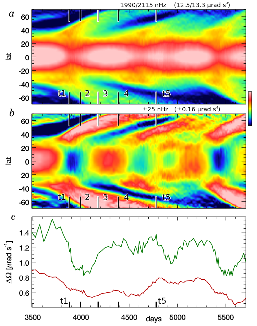
Figure 11.— Time-varying differential rotation in case D5. $(a)$ Time-latitude map of angular velocity $\Omega$ at mid-convection zone ($0.85R_{\odot}$). There are substantial temporal variations at both the equator and high latitudes. $(b)$ These are accentuated by subtracting the time-averaged profile of $\Omega(r,\theta)$ at each latitude. Visible are poleward propagating speedup structures at high latitudes and more uniform modulations near the equator. $(c)$ Corresponding variations in $\Delta\Omega_{\mathrm{lat}}$ near the surface (upper curve, green) and at mid-convection zone (lower, red).

9.1. Bands of Shear

The angular velocity $\Omega$ at mid-convection zone is shown for this period as a time-latitude map in Figure 11$a$. Here again the timing marks indicate our fiducial times t1–t5. In the equatorial regions, the differential rotation remains fast and prograde, but with some modulation in time. Prominent structures of speedup are visible propagating toward the poles at the high latitudes. These structures are much more evident when we subtract the time-averaged profile of $\Omega$ for this period at each latitude (Figure 11$b$). These bands appear as strong, tilted fast (red) bands extending poleward from roughly $\pm 30^{\circ}$ latitude. In the northern hemisphere, three such speedup bands are launched over this interval. In contrast, in the south only two such bands are evident; a third is perhaps launched around day 4500, but it does not survive or propagate.

Comparing these features with the propagation of magnetic fields shown in Figures 5$a$ and 10$a$ over the same interval, we find that velocity speedup features are well correlated with the poleward migration of mean longitudinal magnetic field. The velocity features bear some resemblance to the poleward branch of torsional oscillations observed in the solar convection zone over the course of a solar magnetic activity cycle, though on a much shorter time scale here as befits the correspondingly shorter time between magnetic polarity reversals in these dynamo simulations.

The speedup bands propagate toward the poles relatively slowly. In a period of roughly 500 days they travel about $40^{\circ}$ in latitude, and this angular propagation rate of about $0.08^{\circ}\>\mathrm{day}^{-1}$ or about $1.6\times 10^{-8}\mathrm{rad}\>\mathrm{s}^{-1}$ is roughly constant at all depths in the convection zone. At mid-convection zone ($0.85R_{\odot}$) this corresponds to a distance of roughly 415 Mm and a propagation velocity of about $0.8~{}\mathrm{Mm}\thinspace\thinspace\mathrm{day}^{-1}$ or about $9~{}\mathrm{m}\thinspace\mathrm{s}^{-1}$. Near the base of the convection zone ($0.73R_{\odot}$), this corresponds to a distance of about 355 Mm and a propagation velocity of $0.7~{}\mathrm{Mm}\thinspace\thinspace\mathrm{day}^{-1}$ or about $8~{}\mathrm{m}\thinspace\mathrm{s}^{-1}$.

This is considerably slower than the fluctuating latitudinal flows associated with the convection which at mid-convection zone have peak speeds of $\pm 200~{}\mathrm{m}\thinspace\mathrm{s}^{-1}$ during this time period. The meridional circulations are more difficult to interpret. At mid-convection zone they can have instantaneous amplitudes of about $\pm 10~{}\mathrm{m}\thinspace\mathrm{s}^{-1}$, but the fluctuations are large and the time-averaged circulations are much slower ($\sim 1$–$2~{}\mathrm{m}\thinspace\mathrm{s}^{-1}$) though they are poleward in sense at mid-latitudes. Near the base of the convection zone the time-averaged circulations are weakly equatorward with amplitudes of about $1~{}\mathrm{m}\thinspace\mathrm{s}^{-1}$ and thus act to resist the poleward propagation of the speedup bands and the magnetic wreaths.

If we do moving 35-day time-averages of the meridional flows in the lower convection zone, we see some evidence for variations that track the speedup bands. In particular, the flow in the core of the wreathes tends to be poleward with an amplitude of up to $1$–$3~{}\mathrm{m}\thinspace\mathrm{s}^{-1}$ (up to $5~{}\mathrm{m}\thinspace\mathrm{s}^{-1}$ without smoothing). This poleward flow is likely induced by magnetic tension in the toroidal wreathes, analogous to the mechanism underlying the poleward slip instability (e.g., Moreno-Insertis et al. 1992; Jouve & Brun 2009). In the absence of rotation and convection, the propagation speed associated with the polar slip instability is approximately given by the Alfvén speed associated with the mean toroidal fields,

$$v_{A,\phi}=\frac{\langle B_{\phi}\rangle}{\sqrt{4\pi\bar{\rho}}}.$$ (18)

In case D5, the propagating toroidal features have an amplitude of $\langle B_{\phi}\rangle\sim$ $3$–$6$ kG in the mid convection zone, implying an Alfvén speed of about $30$–$60~{}\mathrm{m}\thinspace\mathrm{s}^{-1}$. Toroidal field strengths are larger near the base of the convection zone, $15$–$25$ kG, yielding larger Alfvén speeds, $\sim 100$–$160~{}\mathrm{m}\thinspace\mathrm{s}^{-1}$, despite the higher density ($0.19~{}\mathrm{g}\thinspace\thinspace\mathrm{cm}^{-3}$, as opposed to $0.065~{}\mathrm{g}\thinspace\thinspace\mathrm{cm}^{-3}$ in the mid convection zone). The much lower poleward flows in the wreathes may reflect the inhibiting influence of rotation (Moreno-Insertis et al. 1992) and convective pumping.

In the lower convection zone, the slip-induced poleward flow must also operate against the background equatorward flow maintained by the convection (Fig. 3$e$). This gives rise to a horizontal convergence of the meridional flow near the poleward edge of each wreath and an associated upward flow with an amplitude of about $1~{}\mathrm{m}\thinspace\mathrm{s}^{-1}$, consistent with mass conservation. This is analogous to the recirculating flows around shear-generated magnetic flux structures that rise due to magnetic buoyancy (e.g., Cline et al. 2003b, a).

In the idealized polar slip instability, the poleward propagation of toroidal bands is associated with the formation of prograde zonal flows as the fluid within the bands tends to conserve its angular momentum. By contrast, the wreathes in case D5 are not isolated flux structures, they have a leaky topology that allows plasma to escape. This will also influence the slip-induced propagation speed but it is likely to accelerate it rather than decelerate it because prograde zonal flows provide gyroscopic stabilization. The wreathes in case D5 do induce prograde zonal flow variations as they migrate poleward (Fig. 11), as expected from the polar slip instability. However, as we shall see in Section 9.2, the zonal flow variations in case D5 are largely produced by the Lorentz force, as opposed to the Coriolis-induced flows associated with angular momentum conservation in closed flux structures.

The important role of the mean Lorentz force in accelerating the torsional oscillations (Section 9.2) and the phasing of the $\Omega$-effect relative to the wreathes (Section 8) suggests that the poleward propagation of the torsional oscillations may be mainly attributed to a nonlinear dynamo wave. The phase speed of such a wave is governed primarily by the poloidal and toroidal source terms in the mean induction equation but it may also be linked to the Alfvén speed associated with the mean latitudinal field. Values of $\langle B_{\theta}\rangle$ in the cores of the poleward propagating bands are roughly $2$–$3$ kG in the mid convection zone, implying Alfvén speeds of about $20$–$30~{}\mathrm{m}\thinspace\mathrm{s}^{-1}$. Near the base of the convection zone these values are larger, with mean latitudinal field strengths of $6$–$9$ kG and Alfvén speeds of $40$–$60~{}\mathrm{m}\thinspace\mathrm{s}^{-1}$.

With the expanded sensitivity of Figure 11$b$, we can see that the equatorial modulation appears as fast and slow pulses which span the latitude range of $\pm 20^{\circ}$. These variations are fairly uniform across this equatorial region. The velocity variations at the equator do not correspond with the equatorial propagating branch of torsional oscillations seen in the Sun (Thompson et al. 2003). In the Sun, the equatorial branch may arise from enhanced cooling in the magnetically active regions (e.g., Spruit 2003; Rempel 2006, 2007).

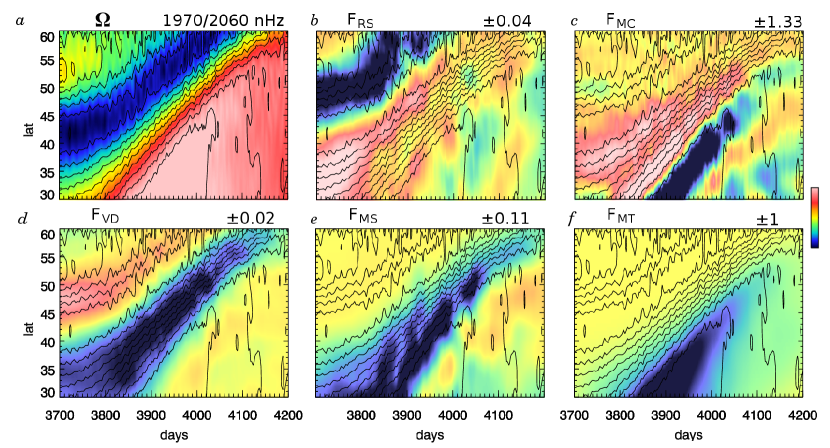
Figure 12.— Angular momentum transport in case D5 in the northern hemisphere of the lower convection zone ($0.73R_{\odot}$). $(a)$ Angular velocity $\Omega$ as image and contour plot in latitude and time. Shown at the same depth, with contours of $\Omega$ overlain to guide comparison, are latitudinal angular momentum fluxes arising from $(b)$ Reynolds stresses ($F_{\mathrm{RS}}$), $(c)$ meridional circulations ($F_{\mathrm{MC}}$), $(d)$ viscous diffusion ($F_{\mathrm{VD}}$), $(e)$ Maxwell stresses from fluctuating fields ($F_{\mathrm{MS}}$), and $(f)$ magnetic torques from axisymmetric fields ($F_{\mathrm{MT}}$). Indicated amplitudes of fluxes are all scaled relative to $F_{\mathrm{MT}}$, with negative (positive) fluxes in the northern (southern) hemisphere representing poleward transport. All fluxes ($b-f$) have been smoothed with a 35-day moving time-average, but the contours of $\Omega$, with no temporal smoothing, give a sense of the variations.

The temporal variations of the angular velocity contrast in latitude $\Delta\Omega_{\mathrm{lat}}$ is shown for this period in Figure 11$c$. At mid-convection zone (sampled by red line) the variations in $\Delta\Omega_{\mathrm{lat}}$ can be substantial, with large contrasts when the fields are strong in the magnetic cycle (prior to t1) and smaller contrasts when the fields are in the process of reversing (t2, t3). Near the surface (green line) $\Delta\Omega_{\mathrm{lat}}$ can show even larger variations. These near-surface values of $\Delta\Omega_{\mathrm{lat}}$ are reported in Table 2, averaged over this entire period (avg) and at points in time when the contrast is large (max, at day 3702) and small (min, at day 4060). From periods of highest contrast to lowest, $\Delta\Omega$ changes by about 0.5 $\mu\mathrm{rad}\>\mathrm{s}^{-1}$, which is a change of roughly 45% relative to the long running average. This corresponds to a total change of about 4% relative to the frame rotation rate of 13 $\mu\mathrm{rad}\>\mathrm{s}^{-1}$ ($5\>\Omega_{\odot}$).

9.2. Angular Momentum Transport

We now turn to discussing the transport of angular momentum associated with the speedup bands observed in case D5. The bands of speedup are clearly associated with the magnetic wreaths which are similarly propagating towards the poles, and here we examine the physical processes that lead to the angular momentum transport that locally speeds up the flow of differential rotation.

Our choice of stress-free and potential-field/perfectly conducting boundary conditions at the top and the bottom of the shell respectively has the advantage that no net external torque is applied and angular momentum is conserved. Convection and magnetism can however redistribute angular momentum throughout the shell. In the general MHD case there are five processes that serve to transport angular momentum (Brun et al. 2004). These are the Reynolds stresses from fluctuating flows (which we denote $F_{\mathrm{RS}}$), the meridional circulations ($F_{\mathrm{MC}}$), the viscous torque ($F_{\mathrm{VD}}$), the Maxwell stresses from fluctuating fields ($F_{\mathrm{MS}}$), and the magnetic torque from the global-scale fields ($F_{\mathrm{MT}}$). The latitudinal component of the angular momentum flux $\cal{F}$ is thus:

$${\cal{F}}_{\theta}=F_{\mathrm{RS}}+F_{\mathrm{MC}}+F_{\mathrm{VD}}+F_{\mathrm{MS}}+F_{\mathrm{MT}},$$ (19)

with

$$F_{\mathrm{RS}} = \bar{\rho}r\sin\theta\langle v_{\theta}^{{}^{\prime}}v_{\phi}^{{}^{\prime}}\rangle,$$ (20)

$$F_{\mathrm{MC}} = \bar{\rho}r\sin\theta\langle v_{\theta}\rangle(\langle{v}_{\phi}\rangle+\Omega_{0}r\sin\theta),$$ (21)

$$F_{\mathrm{VD}} = -\nu\bar{\rho}\sin^{2}\theta\frac{\partial}{\partial\theta}\left(\frac{\langle v_{\phi}\rangle}{\sin\theta}\right),$$ (22)

$$F_{\mathrm{MS}} = -\frac{r\sin\theta}{4\pi}\langle B_{\theta}^{{}^{\prime}}B_{\phi}^{{}^{\prime}}\rangle,$$ (23)

$$F_{\mathrm{MT}} = -\frac{r\sin\theta}{4\pi}\langle{B}_{\theta}\rangle\langle{B}_{\phi}\rangle.$$ (24)

These five latitudinal angular momentum fluxes are displayed for case D5 in Figure 12 along with the angular velocity itself (Figure 12$a$). These measurements are taken in the lower convection zone where the magnetic wreaths are strong (at $0.73R_{\odot}$) and as in Ballot et al. (2007) we do not average these contributions in time but rather follow their time evolution with time-latitude plots. Here we focus on an interval spanning 3700–4200 days when the speedup bands are launched during the reversal. We show only the northern hemisphere here, but dynamics in the southern hemisphere are similar. Contours of angular velocity $\Omega$ are superimposed on each panel to guide the eye.

The transport of angular momentum is modulated and has significant polar branches that are strongly associated with the speedup bands. As the magnetic wreaths propagate poleward, they accelerate the local angular velocity. This is clearly seen in Figure 12$a$, where the latitudinal shear is reduced with the retrograde (blue) regions disappearing as the prograde (red) bands migrate polewards. The acceleration of the high latitude region is largely due to the large-scale magnetic torque associated with the axisymmetric fields in the magnetic wreaths ($F_{\mathrm{MT}}$, Figure 12$f$). This magnetic torque traces the propagation of $\langle B_{\phi}\rangle$ quite well. The negative (positive) sense of this term in the core of the wreaths in the northern (southern) hemisphere indicates that $F_{\mathrm{MT}}$ transports angular momentum toward the poles, thus accelerating flow in those retrograde regions.

The Maxwell stresses from the fluctuating fields ($F_{\mathrm{MS}}$, Figure 12$e$) also help move angular momentum polewards but contribute more weakly than the axisymmetric fields. In the equatorial region $F_{\mathrm{MS}}$ continues to operate even during the reversal when the axisymmetric fields, and hence $F_{\mathrm{MT}}$, are very small. The Reynolds stresses ($F_{\mathrm{RS}}$, Figure 12$b$) generally act to transport angular momentum towards the equator but have amplitudes lower than either of the Maxwell stresses. In this simulation angular momentum transport by viscous diffusion ($F_{\mathrm{VD}}$, Figure 12$d$) plays very little role.

The Coriolis forces associated with the meridional circulations works in concert with the Maxwell torques to spin up the flow in the wreaths ($F_{\mathrm{MC}}$, Figure 12$c$). This spinup largely arises from the poloidal flows associated with the wreaths themselves, rather than from the time-averaged meridional circulations, which are equatorward at this depth. Before the speedup bands begin propagating towards the poles, $F_{\mathrm{MC}}$ is large and opposite in sense to $F_{\mathrm{MT}}$, acting to transport angular momentum towards the equator. In the cores of the wreaths however, $F_{\mathrm{MC}}$ is converging, which acts to spinup the fluid within the wreaths. After the speedup bands have launched (e.g., at about day 3850 in the northern hemisphere), $F_{\mathrm{MC}}$ changes sense and acts to help maintain the prograde rotation in the speedup bands. As the wreaths propagate towards the poles, $F_{\mathrm{MC}}$ is similar in amplitude to $F_{\mathrm{MT}}$ and of the same sense. This large and changing $F_{\mathrm{MC}}$ arises almost entirely from the second term in equation (21); the first term is much smaller in amplitude (roughly 1% of $F_{\mathrm{MT}}$). When no time-averaging is applied, $F_{\mathrm{MC}}$ exhibits large fluctuations on both short and long timescales, with instantaneous amplitudes five or more times larger than $F_{\mathrm{MT}}$.

9.3. Sampling Many Magnetic Cycles in Case D5

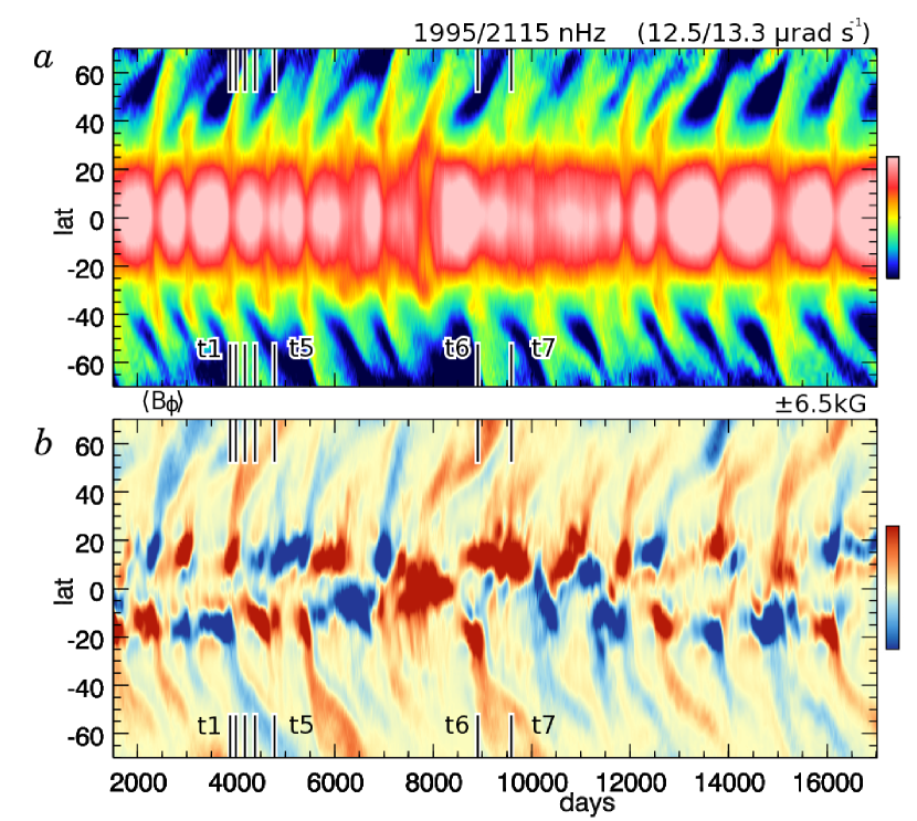
Figure 13.— Extended history of varying differential rotation in case D5. $(a)$ Variations of $\Omega(r,\theta)$ at mid-convection zone. $(b)$ Mean longitudinal field $\langle B_{\phi}\rangle$, at same depth. Poleward propagating speedup structures are visible during each magnetic oscillation. The time samples used in Figures 5 and 14 are indicated.

The linked variations of angular velocity and magnetic fields are shown over considerably longer intervals of time in Figures 13$a,b$. Here too we see the equatorial modulation over many magnetic cycles and the poleward propagating speedup bands. Asymmetries between the northern and southern hemisphere are evident at many times in different cycles. The latitudinal angular velocity contrasts exhibit large variations during each cycle, with $\Delta\Omega_{\mathrm{lat}}$ near the surface ranging from 0.6–1.55 $\mu\mathrm{rad}\>\mathrm{s}^{-1}$ during the interval shown here. Successive magnetic cycles can have distinctly different angular velocity contrasts, and there are additional long-term modulations that span many magnetic cycles. These effects may be very important for stellar observations of differential rotation.

These angular velocity variations are consistently associated with variations in the magnetism. The mean toroidal field $\langle B_{\phi}\rangle$ is shown over the same interval in Figure 13$b$. The poleward propagating magnetic features shown previously in Figures 5$a$ are evident throughout this longer time sampling, now appearing as nearly vertical streaks in $\langle B_{\phi}\rangle$, owing to the compressed time axis. From day 1500 to 7300, four cycles occur in which wreaths of opposite polarity are achieved in each hemisphere. After this period, the dynamo explores unusual single-polarity states. Here either both wreaths have the same polarity (t6) or a single dominant wreath is built (t7). After day 10,700 the dynamo emerges from this state and returns to building two wreaths of opposite polarity which flip in their sense an additional three times as the simulation continues.

10. Strange States and Wreaths of a Single Polarity

Though generally wreaths of opposite polarity are built in each hemisphere, these oscillating dynamos occasionally wander into distinctly different states. This occurs for case D5 around day 7300. Instead of the two nearly antisymmetric wreaths of opposite polarity above and below the equator, the dynamo enters a state where the polarity in each hemisphere is the same, as shown in Figures 14$a,b$ at day 8903. Here two wreaths of same polarity occupy the two hemispheres and persist for an interval of more than 500 days. The positive-polarity $B_{\phi}$ reaches average amplitudes of 18 kG while the weaker negative polarity structures have average amplitudes of only about 3 kG. The azimuthally-averaged profiles of $\langle B_{\phi}\rangle$ emphasize that these wreaths span the convection zone and have the same polarity everywhere. During this interval of time, the mean poloidal field is predominantly quadrupolar.

The dynamo can also achieve states where only a single wreath is built in the equatorial regions, as in Figures 14$c,d$ at day 9590. Here a single strong wreath of positive polarity fills the northern hemisphere, with $\langle B_{\phi}\rangle$ reaching a peak amplitude of +18 kG. This unique structure persists for about 800 days before the dynamo flips polarity and builds a strong wreath of negative polarity. The predecessor of this new wreath can be seen in profiles of $\langle B_{\phi}\rangle$ where a much weaker structure of negative polarity is visible in the lower convection zone.

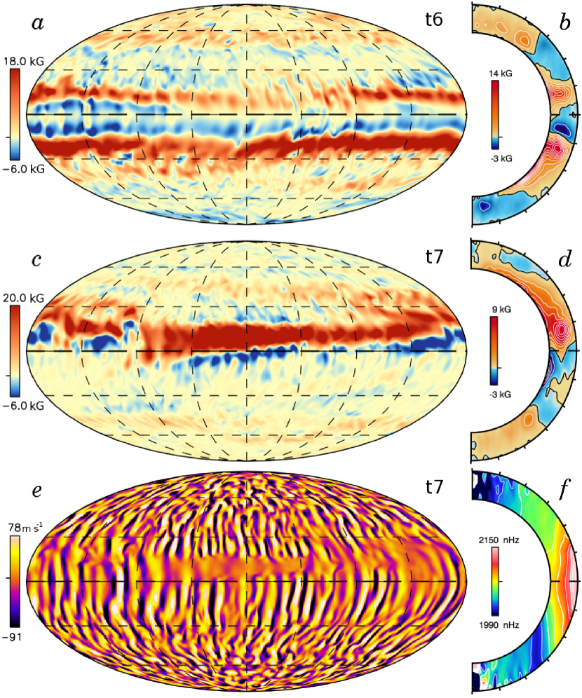
Figure 14.— Strange single-polarity states in case D5 as sampled at times t6 and t7. $(a)$ Snapshot of $B_{\phi}$ at mid-convection zone, showing two strong wreaths of the same polarity. $(b)$ Instantaneous profile of $\langle B_{\phi}\rangle$ at same time. $(c)$ Snapshot of $B_{\phi}$ at mid-convection zone at a time when a single wreath is formed. $(d)$ Weaker negative polarity structures are visible in profile of $\langle B_{\phi}\rangle$ at same instant. $(e)$ Accompanying snapshot of $v_{r}$ at mid-convection zone, showing flows strongly affected by magnetism. $(f)$ The instantaneous differential rotation, shown here as profile of $\Omega(r,\theta)$, is largely unaffected by the strong wreath.

The strong magnetic fields realized in the single wreath states react back on the convective flows. This is evident in the accompanying snapshot of radial velocities at mid-convection zone (Figure 14$e$). In a narrow band spanning $0-20^{\circ}$ latitude and coinciding with the strong tube, the upflows and downflows have been virtually erased. Fluctuations in $v_{\phi}$ and $v_{\theta}$ are also very small in this region, and the flow is dominated by the streaming flows of differential rotation. Within the wreath the total magnetic energy (ME) at mid-convection zone is locally about $10~{}\text{to}~{}100$ times larger than the kinetic energy (KE), while outside the wreath KE exceeds ME by factors of roughly $10~{}\text{to}~{}10^{4}$ at this depth. We see similar restriction of the convective flows whenever the magnetic fields become this strong.

The differential rotation itself (Figure 14$f$) is largely unaffected by the presence of the strong magnetic wreath. There is no clear signature of faster flow down the middle of the wreath. Likewise, there is little sign of the structure in profiles of the thermodynamic variables $P,T,S,$ or $\rho$, with the mean profile instead dominated by latitudinal variations consistent with thermal wind balance.

11. Conclusions

In this paper we have explored dynamo action in a solar-type star rotating five times faster than our Sun currently does. We find that strong dynamo action can occur in the bulk of the convection zone in this rapidly rotating sun and that the resulting magnetic fields are organized on global scales into large wreaths. Generally, these wreaths have opposite polarity in each hemisphere. They are not isolated flux surfaces and instead are intricately linked across the equator and to the polar regions.

This dynamo shows rich time variation, undergoing global-scale magnetic polarity reversals roughly every 1500 days. During a reversal, the magnetic wreaths near the equator propagate towards the poles and are replaced by new wreaths with opposite polarity. Reversals occur in both the mean toroidal field $\langle B_{\phi}\rangle$ and the mean poloidal field. The phasing between the two global-scale fields changes with depth in the convection zone, with the toroidal field changing first in the lower convection zone but the poloidal field reversing first near the surface.

We have analyzed the mechanisms by which the global-scale fields are maintained and destroyed in this dynamo. Generally, we find that the toroidal fields are built primarily by the $\Omega$-effect $P_{\mathrm{MS}}$, where differential rotation stretches the global-scale poloidal magnetic field into mean toroidal field. This generation term generally is well correlated with $\langle B_{\phi}\rangle$, but during a reversal $P_{\mathrm{MS}}$ appears to reverse in sign before the mean fields themselves do. The mean poloidal field is built by the fluctuating emf $E_{\mathrm{FI}}$. This mean contribution arises from correlations in the fluctuating velocities and magnetic fields. Generally, as we found in Paper I, $E_{\mathrm{FI}}$ does not appear to be well represented by a simple $\alpha$-effect where $E_{\mathrm{FI}}$ is given by $\alpha\langle B_{\phi}\rangle$. Rather, $E_{\mathrm{FI}}$ peaks on the poleward edge of the wreaths.

During a reversal, the wreaths from the previous cycle propagate towards the poles. This appears to primarily reflect a dynamo wave, with a poleward-slip instability probably contributing to the dynamics as well. The spatial offset between the primary poloidal and toroidal generation terms, $E_{\mathrm{FI}}$ and $P_{\mathrm{MS}}$ respectively, likely contributes to the poleward propagating dynamo wave behavior which we see here.

Accompanying the poleward propagating magnetic structures are changes in the global-scale differential rotation. Bands of prograde rotating fluid move poleward along with the magnetic wreaths. These speedup bands appear to be accelerated primarily by magnetic torques arising from the global-scale axisymmetric magnetic fields, with an additional contribution arising from poloidal circulations associated with the propagating magnetic wreaths. The angular velocity contrast $\Delta\Omega_{\mathrm{lat}}$ can vary by more than 45% during a reversal and these variations may represent changes of several percent relative to the rotating reference frame. As such, we may expect similar variations in observations of surface differential rotation on magnetically active stars during the course of a magnetic cycle. The bands of speedup bear some resemblance to the poleward branch of the torsional oscillations seen in observations of the Sun over the course of a solar cycle (Thompson et al. 2003). In these simulations, we do not see any evidence of the observed equatorial branch. In the Sun, the equatorial branch may arise from enhanced cooling in the magnetically active regions (e.g., Spruit 2003; Rempel 2006, 2007), but those effects lie beyond the spatial resolution or physical effects included in our simulations of global-scale convection and dynamo action.

These global-scale polarity reversals are not special to case D5. Indeed, we have explored a broader class of oscillating dynamo solutions, which will be detailed in forthcoming papers. Some of these solutions are realized by taking our more slowly rotating case D3 (Paper I) to higher levels of turbulence by reducing the eddy diffusivities, while others are achieved in simulations spinning at even higher rotation rates than case D5. Large oscillations in the magnetic fields and global-scale reversals of polarity appear to be common features in the parameter space we have explored, likely arising when the ohmic diffusivity on large scales is small enough to allow the dynamo waves to run polewards in these wreath-building dynamos. We find such global-scale oscillations and polarity reversals fascinating, since these are self-consistent 3D stellar dynamo simulations which achieve such temporally organized behavior in the bulk of the convection zone, without appealing to a stable tachocline of shear at the base of the convection zone as the organizational seat of the dynamo.

References

- Arfken & Weber (1995) Arfken, G. B. & Weber, H. J. 1995, Mathematical methods for physicists (Academic Press)
- Baliunas et al. (1995) Baliunas, S. L., Donahue, R. A., Soon, W. H., Horne, J. H., Frazer, J., Woodard-Eklund, L., Bradford, M., Rao, L. M., Wilson, O. C., Zhang, Q., Bennett, W., Briggs, J., Carroll, S. M., Duncan, D. K., Figueroa, D., Lanning, H. H., Misch, T., Mueller, J., Noyes, R. W., Poppe, D., Porter, A. C., Robinson, C. R., Russell, J., Shelton, J. C., Soyumer, T., Vaughan, A. H., & Whitney, J. H. 1995, ApJ, 438, 269
- Ballot et al. (2007) Ballot, J., Brun, A. S., & Turck-Chièze, S. 2007, ApJ, 669, 1190
- Bonanno et al. (2006) Bonanno, A., Elstner, D., & Belvedere, G. 2006, Astronomische Nachrichten, 327, 680
- Brown et al. (2008) Brown, B. P., Browning, M. K., Brun, A. S., Miesch, M. S., & Toomre, J. 2008, ApJ, 689, 1354
- Brown et al. (2010) —. 2010, ApJ, 711, 424 (Paper I)
- Browning (2008) Browning, M. K. 2008, ApJ, 676, 1262
- Browning et al. (2007) Browning, M. K., Brun, A. S., Miesch, M. S., & Toomre, J. 2007, Astronomische Nachrichten, 328, 1100
- Browning et al. (2006) Browning, M. K., Miesch, M. S., Brun, A. S., & Toomre, J. 2006, ApJ, 648, L157
- Brun et al. (2005) Brun, A. S., Browning, M. K., & Toomre, J. 2005, ApJ, 629, 461
- Brun et al. (2004) Brun, A. S., Miesch, M. S., & Toomre, J. 2004, ApJ, 614, 1073
- Brun & Toomre (2002) Brun, A. S. & Toomre, J. 2002, ApJ, 570, 865
- Busse (1970) Busse, F. H. 1970, J. Fluid Mech., 44, 441
- Busse (2000) —. 2000, Annual Review of Fluid Mechanics, 32, 383
- Charbonneau (2010) Charbonneau, P. 2010, Living Reviews in Solar Physics, 7, 3:1
- Charbonneau & MacGregor (1997) Charbonneau, P. & MacGregor, K. B. 1997, ApJ, 486, 502
- Christensen & Aubert (2006) Christensen, U. R. & Aubert, J. 2006, Geophysical Journal International, 166, 97
- Cline et al. (2003a) Cline, K. S., Brummell, N. H., & Cattaneo, F. 2003a, ApJ, 599, 1449
- Cline et al. (2003b) —. 2003b, ApJ, 588, 630
- Clune et al. (1999) Clune, T. L., Elliott, J. R., Glatzmaier, G. A., Miesch, M. S., & Toomre, J. 1999, Parallel Computing, 25, 361
- Clyne et al. (2007) Clyne, J., Mininni, P., Norton, A., & Rast, M. 2007, New Journal of Physics, 9, 301
- Dikpati & Charbonneau (1999) Dikpati, M. & Charbonneau, P. 1999, ApJ, 518, 508
- Dikpati & Gilman (2006) Dikpati, M. & Gilman, P. A. 2006, ApJ, 649, 498
- Featherstone et al. (2009) Featherstone, N. A., Browning, M. K., Brun, A. S., & Toomre, J. 2009, ApJ, 328, 1126
- García et al. (2010) García, R. A., Mathur, S., Salabert, D., Ballot, J., Régulo, C., Metcalfe, T. S., & Baglin, A. 2010, Science, 329, 1032
- Ghizaru et al. (2010) Ghizaru, M., Charbonneau, P., & Smolarkiewicz, P. K. 2010, ApJ, 715, L133
- Gilman (1983) Gilman, P. A. 1983, ApJS, 53, 243
- Glatzmaier (1985) Glatzmaier, G. A. 1985, ApJ, 291, 300
- Hall (2008) Hall, J. C. 2008, Living Reviews in Solar Physics, 5, 2:1
- Hempelmann et al. (1996) Hempelmann, A., Schmitt, J. H. M. M., & Stȩpień, K. 1996, A&A, 305, 284
- Jouve et al. (2010) Jouve, L., Brown, B. P., & Brun, A. S. 2010, A&A, 509, A32:1
- Jouve & Brun (2007) Jouve, L. & Brun, A. S. 2007, A&A, 474, 239
- Jouve & Brun (2009) —. 2009, ApJ, 701, 1300
- Käpylä et al. (2010) Käpylä, P. J., Korpi, M. J., Brandenburg, A., Mitra, D., & Tavakol, R. 2010, Astronomische Nachrichten, 331, 73
- Küker et al. (2001) Küker, M., Rüdiger, G., & Schultz, M. 2001, A&A, 374, 301
- Lanza (2010) Lanza, A. F. 2010, in IAU Symposium, Vol. 264, IAU Symposium, ed. A. G. Kosovichev, A. H. Andrei, & J.-P. Roelot, 120–129
- Matt & Pudritz (2008) Matt, S. & Pudritz, R. E. 2008, ApJ, 678, 1109
- Messina & Guinan (2002) Messina, S. & Guinan, E. F. 2002, A&A, 393, 225
- Metcalfe et al. (2010) Metcalfe, T. S., Basu, S., Henry, T. J., Soderblom, D. R., Judge, P. G., Knoelker, M., Mathur, S., & Rempel, M. 2010, ArXiv e-prints
- Miesch et al. (2009) Miesch, M. S., Browning, M. K., Brun, A. S., Toomre, J., & Brown, B. P. 2009, in Astronomical Society of the Pacific Conference Series, Vol. 416, Astronomical Society of the Pacific Conference Series, ed. M. Dikpati, T. Arentoft, I. González Hernández, C. Lindsey, & F. Hill, 443–452
- Miesch et al. (2008) Miesch, M. S., Brun, A. S., DeRosa, M. L., & Toomre, J. 2008, ApJ, 673, 557
- Miesch et al. (2006) Miesch, M. S., Brun, A. S., & Toomre, J. 2006, ApJ, 641, 618
- Mitra et al. (2010) Mitra, D., Tavakol, R., Käpylä, P. J., & Brandenburg, A. 2010, ApJ, 719, L1
- Moreno-Insertis et al. (1992) Moreno-Insertis, F., Schuessler, M., & Ferriz-Mas, A. 1992, A&A, 264, 686
- Muñoz-Jaramillo et al. (2009) Muñoz-Jaramillo, A., Nandy, D., & Martens, P. C. H. 2009, ApJ, 698, 461
- Nandy & Choudhuri (2001) Nandy, D. & Choudhuri, A. R. 2001, ApJ, 551, 576
- Oláh et al. (2009) Oláh, K., Kolláth, Z., Granzer, T., Strassmeier, K. G., Lanza, A. F., Järvinen, S., Korhonen, H., Baliunas, S. L., Soon, W., Messina, S., & Cutispoto, G. 2009, A&A, 501, 703
- Pizzolato et al. (2003) Pizzolato, N., Maggio, A., Micela, G., Sciortino, S., & Ventura, P. 2003, A&A, 397, 147
- Rempel (2005) Rempel, M. 2005, ApJ, 622, 1320
- Rempel (2006) —. 2006, ApJ, 647, 662
- Rempel (2007) —. 2007, ApJ, 655, 651
- Rempel (2008) —. 2008, Journal of Physics Conference Series, 118, 012032.1
- Roberts & Glatzmaier (2001) Roberts, P. H. & Glatzmaier, G. A. 2001, Geophysical and Astrophysical Fluid Dynamics, 94, 47
- Saar & Brandenburg (1999) Saar, S. H. & Brandenburg, A. 1999, ApJ, 524, 295
- Schrijver & De Rosa (2003) Schrijver, C. J. & De Rosa, M. L. 2003, Sol. Phys., 212, 165
- Schrijver & Zwaan (2000) Schrijver, C. J. & Zwaan, C. 2000, Solar and Stellar Magnetic Activity (Cambridge Univsersity Press)
- Shu et al. (1994) Shu, F., Najita, J., Ostriker, E., Wilkin, F., Ruden, S., & Lizano, S. 1994, ApJ, 429, 781
- Spruit (2003) Spruit, H. C. 2003, Sol. Phys., 213, 1
- Spruit & van Ballegooijen (1982) Spruit, H. C. & van Ballegooijen, A. A. 1982, A&A, 106, 58
- Stix (1976) Stix, M. 1976, A&A, 47, 243
- Thompson et al. (2003) Thompson, M. J., Christensen-Dalsgaard, J., Miesch, M. S., & Toomre, J. 2003, ARA&A, 41, 599
- Wang & Sheeley (1991) Wang, Y. & Sheeley, Jr., N. R. 1991, ApJ, 375, 761
- Weber & Davis (1967) Weber, E. J. & Davis, L. J. 1967, ApJ, 148, 217
- Yeates et al. (2008) Yeates, A. R., Nandy, D., & Mackay, D. H. 2008, ApJ, 673, 544
- Yoshimura (1976) Yoshimura, H. 1976, Sol. Phys., 50, 3