• An Improved Metallicity Calibration with UBV Photometry

  S. Karaali^A, S. Bilir^B, S. Ak^B, E. Yaz^B and B. Coşkunoğlu^{B
  A} Beykent University, Faculty of Science and Letters, Department of Mathematics and Computer, Beykent Ayazağa Campus, 34398, Istanbul, Turkey, Email: skaraali@beykent.edu.tr
  ^B Istanbul University, Faculty of Sciences, Department of Astronomy and Space Sciences, 34119 University, Istanbul, Turkey
  

  Abstract: We used the data of 701 stars covering the colour index interval $0.32<B-V\leq 1.16$, with metallicities $-1.76\leq[Fe/H]\leq+0.40$ dex, which were taken from PASTEL catalogue and estimated metallicity dependent guillotine factors which provide a more accurate metallicity calibration. We reduced the metallicities of 11 authors to the metallicities of Valenti & Fischer (2005), thus obtained a homogeneous set of data which increased the accuracy of the calibration, i.e. $[Fe/H]=-14.316\delta^{2}_{0.6}-3.557\delta_{0.6}+0.105$. Comparison of the metallicity residuals, for two sets of data, based on the metallicity dependent guillotine factors with the ones obtained via metal free guillotine factors, shows that metallicities estimated by means of new guillotine factors are more accurate than the other ones. This advantage can be used in the metallicity gradient investigation of the Galactic components, i.e. thin disc, thick disc and halo.

  Keywords: stars: abundances, stars: metallicity calibration, stars: metal poor

1 Introduction

Roman (1955) interpreted the weakness of the metallic lines in the F - and G- type spectra by comparison of the $B-V$ and $U-B$ colours for each star. She stated that an ultraviolet excess, ranging from 0.0 to more than 0.2 mag, which is found in most high -velocity stars, is well correlated with the weakness of the lines. Moreover, both anomalies are correlated with velocity, in the sense that the stars with the weakest lines also have the largest ultraviolet excess and the largest space velocities.

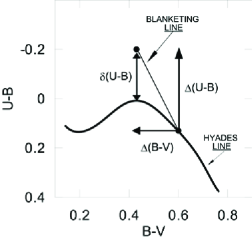
Following Schwarzschild et al. (1955), Sandage & Eggen (1959) interpreted the observed ultraviolet excess for subdwarfs with the “blanketing model”. This model predicts that the change in $B-V$ colour index for a given observed ultraviolet excess, $\delta(U-B)$, for F and G subdwarfs is sufficient to move most of the subdwarfs with known $M_{V}$ on the Hyades main sequence. The essential point of the theory is that the Fraunhofer lines affect the $U$, $B$, and $V$ regions of the spectrum in different ways so that a weakening of the lines produces changes in the observed colour indices: $U-B$ and $B-V$. If the relation between the effect on $U-B$ and $B-V$ is known, then the correction to the observed $B-V$ can be computed from the observed ultraviolet excess. Because the observed $B-V$ for weak line stars will be bluer than that for strong line stars of the same temperature, the weak line stars will fall below the standard main sequence. Therefore, because of the relationship between $\Delta(U-B)$ and $\Delta(B-V)$ we should expect that the displacement of a weak line star below the standard main sequence will be correlated with the observed ultraviolet excess. Wallerstein & Carlson (1960) calibrated the ultraviolet excess in terms of $[Fe/H]$ for the first time, and Wallerstein (1962) improved this calibration. The scheme between the observed ultraviolet excess, $\delta(U-B)$ and the blanketing corrections $\Delta(U-B)$ and $\Delta(B-V)$ (for a hypothetical star) are given in Fig. 1.

The shapes of the blanketing vectors in the $(U-B)-(B-V)$ diagram are such that stars with different $B-V$ values with the same metal abundance will show different ultraviolet excess values. For red stars, $\delta(U-B)$ is partially guillotined because the blanketing line is nearly parallel to the intrinsic Hyades line. If the metal abundances are to be compared among stars of different colours, such as in the works carried out for the estimation of the metallicity gradient for the Galactic fields, corrections to the observed $\delta(U-B)$ are needed. Wildey et al. (1962) provided the basis on which normalized ultraviolet excess was computed by Sandage (1969) and Carney (1979). Sandage (1969) gave a procedure to correct ultraviolet excess values for stars with the same metal abundance, but of different colours for the effect of the guillotine. He plotted 112 stars of large proper motion onto the $(U-B)-(B-V)$ two colour diagram and compared the $U-B$ colours of maximum abundance with that of Hyades for the same $B-V$ colour. The results are given in Table 1. The columns give: (1) $B-V$ colour, (2) the Hyades fiducial line, (3) the maximum $U-B$ value for the sample star for the same $B-V$ of the Hyades star, (4) the $\delta(U-B)$ ultraviolet excess of the sample star in question, and (5) the ratio of the excess at $(B-V)=0.60$ (where $\delta(U-B)$ is maximum), $\delta_{0.6}$, to the excess at any other $B-V$. This ratio is defined as “guillotine factor” in this paper, i.e. $f_{S}=\delta_{0.6}/\delta(U-B)$, where the subscript “$S$” refers to Sandage. Table 1 gives the guillotine factors of Sandage (1969) for a set of 16 colours with 0.35$\leq$$B-V$$\leq$1.10. One can estimate guillotine factors for a larger set of $B-V$ colours by applying an interpolation formula to the data in Table 1. This is the case in some of our works (Karaali et al. 2003; Ak et al. 2007a, b; Yaz & Karaali 2010).

Table 1: The guillotine factors of Sandage (1969). The symbols are explained in the text.

$B-V$	$(U-B)_{H}$	$(U-B)_{M}$	$\delta(U-B)$	$\delta_{0.6}/\delta(U-B)$
0.35	0.03	-0.22	0.25	1.24
0.40	0.01	-0.25	0.26	1.19
0.45	0.00	-0.27	0.27	1.15
0.50	0.03	-0.25	0.28	1.11
0.55	0.08	-0.22	0.30	1.03
0.60	0.13	-0.18	0.31	1.00
0.65	0.19	-0.11	0.30	1.03
0.70	0.25	-0.03	0.28	1.10
0.75	0.34	0.08	0.26	1.19
0.80	0.43	0.19	0.24	1.29
0.85	0.54	0.32	0.22	1.41
0.90	0.64	0.44	0.20	1.55
0.95	0.74	0.55	0.19	1.63
1.00	0.84	0.67	0.17	1.82
1.05	0.94	0.79	0.15	2.06
1.10	0.99	0.87	0.12	2.58

Figure 1: The scheme between the observed ultraviolet excess, $\delta(U-B)$ and the blanketing corrections $\Delta(U-B)$ and $\Delta(B-V)$ taken from Sandage & Eggen (1959).

Carney (1979) normalized the ultraviolet excesses of 101 dwarfs by using the procedure of Sandage (1969) and calibrated them to the metal abundance $[Fe/H]$. This calibration could be used to evaluate metal abundances in the $UBV$ photometry. Karaali et al. (2003) improved this calibration by using a different procedure and a different set of $UBV$ data. Other works in different photometries followed the ones carried out in the $UBV$ for metallicity estimation. Buser & Fenkart (1990) calibrated the $[Fe/H]$ metal abundance to the normalized $\delta(U-G)$ excess and $(G-R)$ colour, simultaneously, in the $RGU$ photometry. Strömgren (1966) defined the $m_{1}=(v-b)-(b-y)$ colour difference as a metallicity indicator, where $v$, $b$, and $y$ are magnitudes for intermediate bands in his $uvby-\beta$ photometry and the $(B-L)$ colour turned out to be a very sensitive metallicity index for F- G spectral type stars in the $VBLUW$ photometry (Walraven & Walraven 1960; Trefzger et al. 1995).

There are deviations between the calibrations obtained for the $UBV$ system. Fig. 15 of Buser & Kurucz (1992) compares these calibrations based on empirical data (Carney 1979; Cameron 1985) or theoretical models (Buser & Kurucz 1978, 1985; Vandenberg & Bell 1985). The reason for these differences originates from two sources: 1) Although researchers use the $UBV$ data of the same stars, the references and hence the $UBV$ magnitudes or colours therein may be different. 2) Different atmospheric parameters may be used by different researchers in estimation of the metallicities used for $[Fe/H]-\delta_{0.6}$ calibration (cf. Cayrel de Strobel et al. 2001).

The guillotine factors of Sandage (1969) are colour dependent, but not metallicity dependent. However, the isometallicity lines in the $(U-B)-(B-V)$ two colour diagram are not parallel to each other for the whole colour range of $B-V$ which indicates the dependence of the guillotine factors on the metallicity. This is the main topic of the paper. The data are presented in Section 2. The guillotine factors and the metallicity calibration are given in Section 3 and finally a short discussion is presented in Section 4.

2 The data

The PASTEL catalogue (Soubiran et al. 2010) is the main source of data for our study. 4259 stars with $4\leq\log g\leq 5$ and with known metallicity and metallicity errors were selected as main sequence stars from the PASTEL catalogue. 3187 out of these stars that were not displaying a variability in their magnitudes which were tagged as “star”, “star in cluster” and “high proper motion stars” in SIMBAD were used in the study. To obtain $UBV$ data, we consulted the specialized catalogues which are included in the General Catalogue of Photometric Data (Hauck et al. 1990), which provided the data of 2073 stars.

To calibrate the metallicity more accurately, we selected 11 authors appearing in the PASTEL catalogue (Soubiran et al. 2010), whose databases coincide the most with the 2073 stars in our study. These authors are: Valenti & Fischer (2005), Sousa et al. (2008), Ramirez & Melendez (2005), Santos et al. (2004), Fuhrmann (2008), Luck & Heiter (2006), Mishenina et al. (2004), Nissen et al. (2002), Ryan & Smith (2003), Spite et al. (1996) and Tomkin & Lambert (1999). From all authors we collected a total of 701 stars of which Valenti & Fischer (2005) determined the metal abundances of 472 stars. Hence, we reduced all the metallicities to Valenti & Fischer (2005)’s using the calibrations between the metal abundances of common stars in the work of Valenti & Fischer (2005) and other researchers. Table 2 gives the resulting star catalogue obtained by this procedure. The errors cited for the metal abundances belong to the original ones. The parallaxes were taken from the newly reduced Hipparcos catalogue (van Leeuwen 2007). The $UBV$ data of stars in Table 2 have been dereddened by the following procedure (Bahcall & Soneira 1980).

$$A_{d}(b)=A_{\infty}(b)\times(1-e^{\frac{-|d\sin(b)|}{H}})$$ (1)

Here $b$ and $d$ are the Galactic latitude and the distance of the star (evaluated by means of its parallax), respectively. $H$ is the scaleheight for the interstellar dust which is adopted as 125 pc (Marshall et al. 2006) and $A_{\infty}(b)$ and $A_{d}(b)$ are the total absorptions for the model (Schlegel et al. 1998) and for the distance to the star respectively. $A_{\infty}(b)$ can be evaluated by means of Eq. 2

$$A_{\infty}(b)=3.1\times E(B-V),$$ (2)

where $E_{\infty}(B-V)$ is the colour excess for the model taken from NASA Extragalactic Database. Then, $E_{d}(B-V)$, i.e. the colour excess for the corresponding star at the distance $d$ can be evaluated by Eq. 2 adopted for distance $d$

$$E_{d}(B-V)=A_{d}(b)/3.1,$$ (3)

and can be used for the colour excess $E_{d}(U-B)$ evaluation:

$$E_{d}(U-B)=0.72E_{d}(B-V)+0.05E_{d}^{2}(B-V).$$ (4)

Finally, the dereddened colour indices are:

$$(B-V)_{0}=(B-V)-E_{d}(B-V)$$ (5)

$$(U-B)_{0}=(U-B)-E_{d}(U-B).$$

The reduced ultraviolet excess $\delta_{0.6}$ is evaluated by the following equation which is obtained by the data of 133 stars with $0.575\leq(B-V)\leq 0.625$ (Table 3):

$$\delta_{0.6}=-0.038(0.005)[Fe/H]^{3}-0.163(0.019)[Fe/H]^{2}$$ (6)

$$-0.302(0.017)[Fe/H]+0.012(0.004).$$

In this study, Karaali’s guillotine factor is denoted by “$f_{K}$” and is calculated with $f_{K}=\delta_{0.6}/\delta$.

Table 2: Data used for metallicity calibration. The columns give: CD, BD, HD or G (Giclas) number, ($\alpha$, $\delta$) and ($l$, $b$) equatorial and Galactic coordinates, distance (pc), dereddened $UBV$ data, reduced ultraviolet excess $\delta_{0.6}$, original metallicity $[Fe/H]$ and its error, metallicity reduced to Valenti & Fischer (2005) system $[Fe/H]_{VF}$ and the author. The coordinates are defined as in ICRS.

Star	$\alpha$	$\delta$	$l$	$b$	$d$	$V_{o}$	$(B-V)_{o}$	$(U-B)_{o}$	$\delta_{0.6}$	$[Fe/H]$	$[Fe/H]_{err}$	$[Fe/H]_{VF}$	Author
HD000055	00 05 17.670	-67 49 57.73	309.497	-48.703	16	8.486	1.062	0.863	0.15	-0.66	0.02	-0.64	Sousa
HD000101	00 05 54.739	+18 14 05.83	108.005	-43.313	37	7.431	0.554	0.036	0.08	-0.28	0.04	-0.25	Ramirez
HD000142	00 06 19.215	-49 04 30.76	321.587	-66.387	26	5.694	0.514	0.021	-0.03	0.10	0.03	0.14	Valenti
HD000283	00 07 32.507	-23 49 07.50	48.982	-79.560	33	8.675	0.795	0.336	0.13	-0.55	0.03	-0.52	Valenti
HD000400	00 08 40.373	+36 37 37.76	113.443	-25.426	32	6.155	0.486	-0.070	0.06	-0.21	0.03	-0.18	Valenti
…	…	…	…	…	…	…	…	…	…	…	…	…	…
…	…	…	…	…	…	…	…	…	…	…	…	…	…
…	…	…	…	…	…	…	…	…	…	…	…	…	…
HD223498	23 50 05.768	+02 52 38.04	94.302	-56.546	45	8.305	0.733	0.354	-0.08	0.23	0.03	0.27	Valenti
HD224022	23 54 38.598	-40 18 00.16	341.042	-72.356	28	6.013	0.572	0.106	-0.05	0.15	0.06	0.19	Sousa
HD224156	23 55 32.411	+03 30 04.95	97.015	-56.531	30	7.685	0.746	0.346	0.01	-0.03	0.03	0.00	Valenti
HD224383	23 57 33.478	-09 38 50.59	84.366	-68.386	48	7.826	0.629	0.137	0.02	-0.04	0.03	-0.01	Valenti
HD224619	23 59 28.388	-20 02 05.06	60.981	-76.155	25	7.456	0.740	0.281	0.06	-0.20	0.01	-0.17	Sousa

3 Methods

3.1 New Guillotine Factors

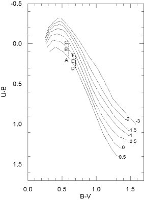
Sandage (1969) estimated guillotine factors without considering the effect of metallicity. However, Fig. 2 shows that the colour gradients for any two different isometallicity lines are not equal to each other, i.e. $\frac{|AB|}{|DE|}\neq\frac{|AC|}{|DF|}$, which indicates the dependence of guillotine factors on metallicity. Additionally, the $(U-B)_{M}$ colours in Table 1 correspond to the stars with less metallicity than the Hyades cluster. But, the metallicity gradients for the isometallicity line with $[Fe/H]=0.5$ dex in Fig. 2 are rather different than the ones for relatively metal poor stars which indicates that guillotine factors for metal rich stars should be different than those of metal poor stars of the same $B-V$ colour index.

Figure 2: Synthetic isometallicity lines for $UBV$ photometry taken from a stellar model of Lejeune et al. (1997).

Figure 3: Metallicity versus ultraviolet excess calibration for 133 stars with $0.575\leq B-V\leq 0.625$.

Table 3: Stars with $0.575\leq B-V\leq 0.625$ used for calibration of $\delta_{0.6}$ to metallicity. Symbols are the same with Table 2.

Star	$(B-V)_{o}$	$(U-B)_{o}$	$[Fe/H]$	$\delta_{(0.6)}$	Star	$(B-V)_{o}$	$(U-B)_{o}$	$[Fe/H]$	$\delta_{(0.6)}$	Star	$(B-V)_{o}$	$(U-B)_{o}$	$[Fe/H]$	$\delta_{(0.6)}$
HD020407	0.576	-0.023	-0.42	0.128	HD155918	0.592	-0.017	-0.64	0.139	HD221146	0.611	0.214	0.11	-0.070
HD043745	0.577	0.078	0.13	0.028	HD024040	0.593	0.198	0.21	-0.074	HD010519	0.612	0.027	-0.58	0.118
HD003149	0.578	0.061	-0.07	0.046	HD039091	0.593	0.094	0.05	0.030	HD013043	0.612	0.145	0.09	0.000
HD134088	0.578	-0.059	-0.75	0.166	HD102158	0.593	0.038	-0.47	0.086	HD033021	0.612	0.080	-0.14	0.065
HD104800	0.578	-0.059	-0.82	0.166	HD196800	0.593	0.137	0.16	-0.013	HD084737	0.612	0.143	0.17	0.002
HD145809	0.578	0.057	-0.24	0.050	HD221830	0.593	0.057	-0.40	0.067	HD054351	0.613	0.115	-0.05	0.031
HD188510	0.578	-0.131	-1.64	0.238	HD061383	0.594	0.024	-0.48	0.101	HD064090	0.614	-0.129	-1.80	0.276
BD+660268	0.580	-0.147	-2.09	0.257	BD+730943	0.594	0.016	-0.37	0.109	HD030562	0.614	0.181	0.26	-0.034
HD286891	0.580	-0.040	-0.56	0.150	HD070110	0.594	0.142	0.15	-0.017	HD068978	0.614	0.067	0.02	0.080
HD030649	0.580	0.029	-0.49	0.081	HD088986	0.594	0.156	0.09	-0.031	HD139324	0.614	0.156	0.15	-0.009
HD078366	0.580	0.039	0.08	0.071	HD096700	0.594	0.065	-0.18	0.060	HD094835	0.615	0.116	0.13	0.032
HD126681	0.581	-0.115	-1.16	0.226	HD009782	0.595	0.086	0.09	0.040	HD178496	0.615	0.119	-0.26	0.029
HD029461	0.581	0.145	0.25	-0.034	HD009782	0.595	0.086	0.15	0.040	HD120066	0.615	0.147	0.11	0.001
HD006500	0.582	-0.009	-0.60	0.121	HD045391	0.595	0.016	-0.50	0.110	HD166435	0.615	0.086	0.04	0.062
HD007983	0.582	-0.028	-0.60	0.140	HD073524	0.595	0.116	0.12	0.010	BD+591609	0.616	0.070	-0.45	0.079
HD115383	0.582	0.093	0.28	0.019	HD067458	0.596	0.036	-0.19	0.091	HD003074	0.616	0.146	0.00	0.003
HD196850	0.582	0.071	-0.11	0.041	HD110898	0.597	0.009	-0.38	0.119	HD066171	0.616	0.057	-0.31	0.092
HD199288	0.582	-0.045	-0.63	0.157	HD004307	0.597	0.069	-0.19	0.059	HD208704	0.617	0.109	-0.08	0.041
HD165499	0.583	0.055	0.01	0.058	HD020807	0.598	0.001	-0.26	0.128	HD152792	0.617	0.091	-0.31	0.059
HD044120	0.583	0.080	0.10	0.033	HD143761	0.598	0.083	-0.20	0.046	HD250792	0.618	-0.043	-1.07	0.195
HD133161	0.583	0.165	0.21	-0.052	HD150433	0.599	0.047	-0.38	0.083	HD001832	0.618	0.121	-0.03	0.031
HD158226	0.584	-0.028	-0.52	0.142	HD070923	0.600	0.097	0.12	0.034	HD008262	0.618	0.091	-0.16	0.061
BD+592407	0.584	-0.103	-1.95	0.217	HIP043595	0.600	-0.040	-0.80	0.171	HD051419	0.618	0.069	-0.40	0.083
HD171990	0.585	0.114	0.07	0.001	HD006434	0.600	-0.012	-0.52	0.143	HD053705	0.618	0.045	-0.21	0.107
HD083529	0.585	0.019	-0.25	0.096	HD150706	0.600	0.076	-0.01	0.055	HD097998	0.619	0.052	-0.41	0.101
HD206332	0.585	0.169	0.27	-0.054	HD088218	0.600	0.148	-0.14	-0.017	HD216435	0.619	0.169	0.24	-0.016
HD059360	0.586	0.087	-0.12	0.029	HD088725	0.600	-0.016	-0.70	0.147	HD036283	0.620	0.083	-0.31	0.071
HD129290	0.586	0.062	-0.13	0.054	HD107146	0.600	0.071	-0.03	0.060	HD031966	0.621	0.215	0.13	-0.060
HD018709	0.586	-0.003	-0.26	0.119	HD090508	0.601	0.054	-0.30	0.078	HD038858	0.621	0.086	-0.23	0.069
HD131117	0.586	0.087	0.14	0.029	HD165401	0.601	0.021	-0.36	0.111	HD034411	0.622	0.121	0.12	0.035
HD170778	0.586	0.087	0.00	0.029	HD222033	0.601	0.121	0.19	0.011	HD071148	0.622	0.118	0.02	0.038
HD014056	0.587	-0.012	-0.61	0.129	HD010226	0.602	0.134	0.22	0.000	HD071881	0.622	0.134	-0.05	0.022
HD111367	0.587	0.086	-0.18	0.031	HD211415	0.603	0.059	-0.20	0.076	HD183658	0.623	0.158	0.05	-0.001
G 232-18	0.587	-0.019	-0.80	0.136	HD218209	0.604	0.049	-0.46	0.087	HD042618	0.624	0.119	-0.11	0.040
HD124553	0.587	0.143	0.28	-0.026	HD056274	0.605	-0.018	-0.55	0.155	HD088371	0.624	0.109	-0.31	0.050
HD093745	0.587	0.111	0.08	0.006	HD073668	0.605	0.079	0.00	0.058	HD199960	0.624	0.213	0.27	-0.054
HD041330	0.588	0.051	-0.14	0.067	HD095128	0.605	0.123	0.04	0.014	HD018757	0.625	0.128	-0.28	0.032
HD019373	0.588	0.113	0.16	0.005	HD164427	0.605	0.117	0.13	0.020	CD-2808426	0.625	0.019	-0.64	0.141
HD052711	0.588	0.058	-0.10	0.060	HD197076	0.607	0.071	-0.09	0.068	HD147231	0.625	0.216	0.00	-0.056
HD168871	0.588	0.046	-0.09	0.072	HD009224	0.608	0.108	0.00	0.032	HD179140	0.625	0.162	0.12	-0.002
HD088742	0.589	0.073	-0.05	0.046	HD149612	0.608	0.024	-0.45	0.116	HD196068	0.625	0.273	0.31	-0.113
HD283807	0.590	0.000	-0.58	0.120	HD114729	0.609	0.044	-0.26	0.097	HD200565	0.625	0.112	-0.06	0.048
HD121004	0.591	-0.056	-0.80	0.177	HD118475	0.609	0.166	0.10	-0.025	BD+38 4955	0.660	-0.160	-2.50	0.340
HD001388	0.591	0.088	0.00	0.033	HD223238	0.609	0.128	0.02	0.013
HD016623	0.591	0.007	-0.45	0.114	HD134060	0.610	0.139	0.09	0.003

Figure 4: $(U-B)-(B-V)$ two colour diagram for the whole sample (a) and for 50 bins of eight subsamples in Table 4 (b).

Figure 5: Calibration of ultraviolet excess ($\delta$) to the guillotine factor $f_{K}$ for eight subsamples.

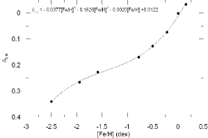
Then we decided that it should be more appropriate and useful to estimate metallicity dependent guillotine factors. First, we used 133 stars with colour index $0.575\leq B-V\leq 0.625$ and calibrated their ultraviolet excess to the metallicity. The calibration (Eq. 6) provides ultraviolet excess reduced to $B-V=0.60$ for any star with metal abundance $[Fe/H]\geq-2.5$ dex. Thus, we can use the calibration obtained from Fig. 3 to estimate reduced $\delta_{0.6}$ ultraviolet excess for stars with metal abundance $-2.5\leq[Fe/H]\leq 0.15$ dex.

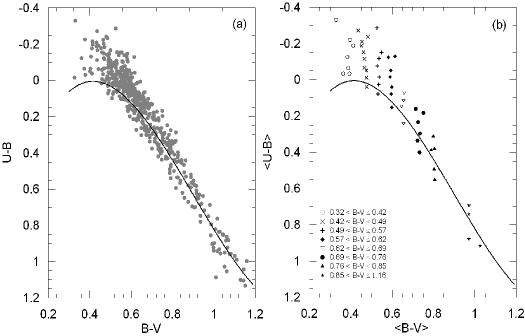
Next, we separated the stars in Table 2 into eight subsamples with colour indices $0.32<B-V\leq 0.42$, $0.42<B-V\leq 0.49$, $0.49<B-V\leq 0.57$, $0.57<B-V\leq 0.62$, $0.62<B-V\leq 0.69$, $0.69<B-V\leq 0.76$, $0.76<B-V\leq 0.85$, $0.85<B-V\leq 1.16$ and obtained calibrations for the guillotine factors as explained in the following: The number of these colour intervals and their ranges had been decided such as to obtain a constant metallicity gradient for each $B-V$ interval. For example, the ranges for bluer stars, where the metallicity gradient is relatively large were adopted smaller than for the colour interval, $0.85<B-V\leq 1.16$, where the metallicity gradient is rather smooth. The $(U-B)-(B-V)$ colour diagrams of the whole sample and eight subsamples are shown in Fig. 4.

Each subsample was divided into bins and mean $\delta$, $B-V$, $U-B$, $[Fe/H]$, $(U-B)_{H}$, $\delta_{0.6}$ and $f_{K}$ values were evaluated for each subsample (Table 4). A total of 532 stars could be used in the calibration of guillotine factors. Ultraviolet -excess $\delta$ of a sample star whose $U-B$ colour index is close to that of a Hyades star of the same $B-V$ colour index is rather small. Hence, $f_{K}$=$\delta_{0.6}$/$\delta$ becomes rather large for such stars and they are not reliable. These abnormal $f_{K}$ values may be as large as 20, for example. Also, we noted that the $f_{K}$ values of some stars were negative. The reason of these unreliable values originate from the errors in $U-B$ colour index. After rejection the stars with large and negative $f_{K}$ values the number of stars reduced from 701 to 532. The numbers of stars used in each bin is given in the last column of Table 4.

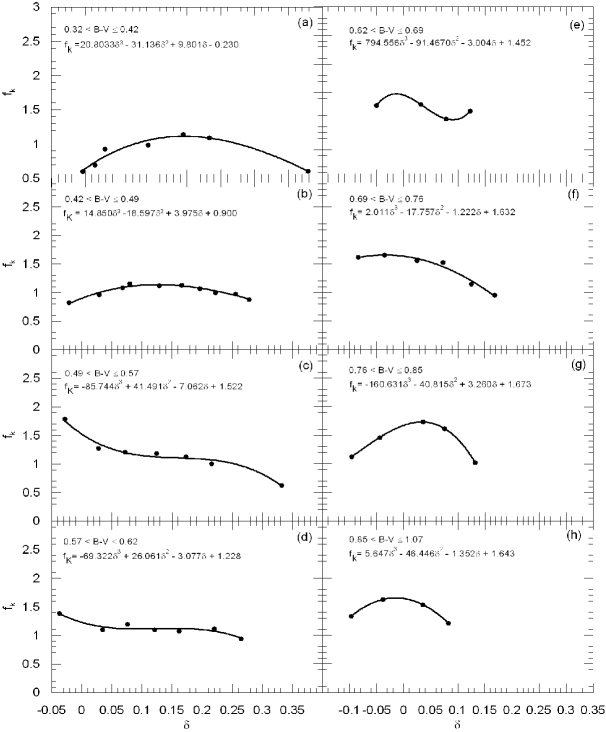
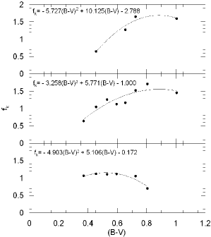
The calibration of $\delta$ to $f_{K}$ is given in Fig. 5. One notices that there is a smooth relation in all panels, and the trend of the guillotine factor varies in different panels. In panels (a), (b), (g) and (h), $f_{K}$ assumes its maximum at the intermediate values of $\delta$, whereas in panels (c), (d), (e) and (f) the maximum of $f_{K}$ corresponds to the negative values of $\delta$, i.e. metal rich stars. Fig. 6 shows the calibration of $B-V$ to $f_{K}$ for three ultraviolet excess, i.e. $\delta=-0.05$, +0.05 and +0.15, just to show that one can obtain continuous transitions between colour index and ultraviolet excess. Since Fig. 5 is divided according to colours and the fits are in better agreement with data, the obtained equations will be more precise. Therefore, we prefer the equations obtained from Fig. 5.

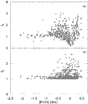
Fig. 7 shows the distribution of the guillotine factors as a function of metallicity. The lower limit for the guillotine factors of Sandage (1969) is $f_{S}=1$ (panel b), corresponding to the colour index $B-V=0.60$, whereas the one estimated in this work which may be less than 0.5, which is not colour dependent, but corresponds to metal abundance $[Fe/H]\approx 0$ dex.

Table 4: Ultraviolet excess $\delta$, reduced ultraviolet excess $\delta_{0.6}$ and new guillotine factors $f_{K}$ for each bin of eight sub -samples. The symbols are explained in the text.

$\langle B-V\rangle$	$\langle U-B\rangle$	$\langle[Fe/H]\rangle$	$\langle(U-B)_{H}\rangle$	$\delta$	$\delta_{0.6}$	$f_{K}$	N
$0.32<B-V\leq 0.42$
0.394	-0.034	-0.053	0.012	0.046	0.028	0.595	2
0.364	-0.033	-0.110	0.031	0.064	0.043	0.695	2
0.388	-0.064	-0.224	0.014	0.079	0.071	0.924	2
0.384	-0.126	-0.584	0.017	0.143	0.140	0.985	2
0.412	-0.188	-1.424	0.008	0.195	0.221	1.135	2
0.396	-0.220	-1.836	0.012	0.233	0.254	1.092	2
0.329	-0.330	-1.530	0.050	0.379	0.229	0.603	1
$0.42<B-V\leq 0.49$
0.477	0.039	0.082	0.018	-0.021	-0.014	0.819	3
0.475	-0.012	-0.054	0.017	0.029	0.027	0.964	6
0.475	-0.051	-0.228	0.017	0.068	0.073	1.082	2
0.466	-0.066	-0.307	0.014	0.080	0.090	1.152	4
0.466	-0.115	-0.633	0.014	0.129	0.145	1.119	4
0.462	-0.153	-0.981	0.013	0.166	0.187	1.128	4
0.452	-0.186	-1.268	0.010	0.196	0.210	1.072	6
0.455	-0.211	-1.443	0.011	0.222	0.223	1.003	3
0.482	-0.237	-1.763	0.019	0.256	0.249	0.973	2
0.436	-0.271	-1.745	0.007	0.278	0.244	0.879	1
$0.49<B-V\leq 0.57$
0.532	0.080	0.188	0.052	-0.028	-0.053	1.787	12
0.535	0.026	-0.085	0.054	0.028	0.036	1.273	24
0.537	-0.016	-0.307	0.056	0.072	0.087	1.209	38
0.528	-0.075	-0.641	0.049	0.124	0.146	1.182	27
0.536	-0.117	-1.069	0.056	0.173	0.194	1.127	10
0.549	-0.150	-1.414	0.065	0.216	0.217	1.006	4
0.526	-0.286	-1.211	0.046	0.332	0.206	0.623	1
$0.57<B-V\leq 0.62$
0.598	0.153	0.161	0.116	-0.037	-0.042	1.387	19
0.595	0.078	-0.096	0.113	0.035	0.039	1.098	23
0.598	0.041	-0.321	0.117	0.076	0.089	1.195	29
0.590	-0.015	-0.546	0.107	0.121	0.133	1.097	21
0.593	-0.051	-0.850	0.111	0.162	0.174	1.073	5
0.581	-0.124	-1.710	0.096	0.220	0.245	1.112	4
0.614	-0.129	-1.801	0.136	0.265	0.249	0.941	1
$0.62<B-V\leq 0.69$
0.655	0.243	0.201	0.192	-0.050	-0.057	1.274	34
0.645	0.147	-0.111	0.179	0.032	0.042	1.288	22
0.655	0.115	-0.276	0.193	0.078	0.081	1.038	29
0.658	0.073	-0.611	0.196	0.123	0.143	1.177	12
$0.69<B-V\leq 0.76$
0.732	0.401	0.387	0.317	-0.084	-0.133	1.611	6
0.722	0.335	0.218	0.300	-0.035	-0.064	1.650	13
0.734	0.296	-0.098	0.321	0.025	0.038	1.555	11
0.726	0.234	-0.429	0.306	0.073	0.109	1.525	17
0.714	0.161	-0.604	0.286	0.125	0.141	1.143	4
0.751	0.183	-0.886	0.351	0.168	0.164	0.955	2
$0.76<B-V\leq 0.85$
0.806	0.550	0.328	0.454	-0.096	-0.106	1.127	5
0.803	0.491	0.220	0.447	-0.044	-0.063	1.461	10
0.789	0.385	-0.175	0.422	0.036	0.060	1.737	11
0.805	0.378	-0.458	0.453	0.075	0.117	1.614	17
0.799	0.308	-0.583	0.440	0.132	0.134	1.024	8
$0.85<B-V\leq 1.16$
0.972	0.878	0.360	0.782	-0.097	-0.121	1.332	11
1.025	0.915	0.215	0.877	-0.038	-0.062	1.627	11
0.971	0.741	-0.165	0.776	0.035	0.055	1.539	21
0.971	0.693	-0.373	0.777	0.083	0.100	1.214	22

Figure 6: Calibration of $B-V$ colour to the guillotine factor $f_{K}$ for three ultraviolet excesses, $\delta=-0.05$, +0.05, and +0.15.

Figure 7: Guillotine factors versus metallicity: (a) for metallicity dependent guillotine factors ($f_{K}$); (b) for guillotine factors free of metallicity given by Sandage (1969)($f_{S}$).

Figure 8: Metallicity calibration based on the metallicity dependent guillotine factors (a) and the ones adopted from Sandage (1969) (b). The dashed lines denote the $\pm 1\sigma$ prediction levels.

3.2 New Metallicity Calibration

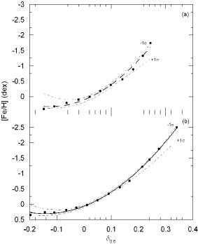
We used the calibrations in Fig. 5 and assigned guillotine factors, $f_{K}$, for 701 stars with metallicity $-1.76\leq[Fe/H]\leq+0.40$ dex. The combinations of $f_{K}$ and the ultraviolet excess $\delta$ gives the reduced ultraviolet excess for each star, i.e. $\delta_{0.6}=f_{K}\times\delta$. Then we divided the interval $-0.15\leq\delta_{0.6}\leq 0.24$ into 11 scans and adopted the centroid of each scan as a locus point to fit a second order polynomial (Fig. 8) to the couple ($\delta_{0.6}$, $[Fe/H]$). The full equation of the polynomial is

$$[Fe/H]=-14.316(1.919)\delta_{0.6}^{2}+3.557(0.285)\delta_{0.6}$$ (7)

$$+0.105(0.039).$$

Eq. 7 provides metallicities by means of new guillotine factors. We used the guillotine factors of Sandage (1969) and evaluated another set of reduced $\delta_{0.6}$ ultraviolet excess for the same star sample. Their fit to the corresponding metallicities is given in Fig. 8 and in the following formula:

$$[Fe/H]=-11.612(0.496)\delta_{0.6}^{2}+3.419(0.100)\delta_{0.6}$$ (8)

$$+0.057(0.017).$$

3.3 Application of the Method

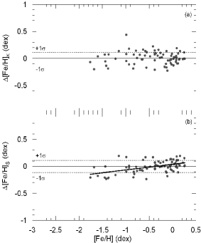
Now, we have two metallicity calibrations, based on the new guillotine factors estimated in this work and on the guillotine factors adopted from Sandage (1969). We applied these calibrations to two sets of data with $-1.76\leq[Fe/H]\leq 0.4$ dex taken from Karaali et al. (2003) and Karataş & Schuster (2006) and we compared the evaluated metallicities with the original ones for two calibrations. The metallicities of 75 stars in the first set were estimated spectroscopically, whereas those for 469 stars are based on photometry. Stars in two sets just mentioned and the sample stars do not overlap. The results for the data of Karaali et al. (2003) are given in Table 5. The clarification of the symbols is as follows: Hip No: the Hipparcos number, $\delta$ the ultraviolet excess, $f_{K}$ and $f_{S}$: the guillotine factors estimated in this work and adopted from Sandage (1969), respectively, $\delta_{0.6}(K)$ and $\delta_{0.6}(S)$: ultraviolet excess reduced by means of $f_{K}$ and $f_{S}$, respectively, $[Fe/H]_{obs}$, $[Fe/H]_{K}$ and $[Fe/H]_{S}$: original metallicities taken from the literature and metallicities evaluated via Eqs. 7 and 8, respectively, $\Delta[Fe/H]_{K}$ and $\Delta[Fe/H]_{S}$: residuals for two calibrations, where $K$ and $S$ refer to the data evaluated by means of the guillotine factors estimated in this work and the ones adopted from Sandage (1969). The results for 469 stars are not given here in order to avoid space consuming. However, their statistics are given in Table 6 together with the ones of 75 stars in the first set.

Comparison of the mean and standard deviations for the residuals of two calibrations for four metallicity intervals, i.e. $-1.76<[Fe/H]\leq-1$, $-1<[Fe/H]\leq-0.5$, $-0.5<[Fe/H]\leq 0$ and $0<[Fe/H]\leq+0.4$ dex shows that there are statistical differences between two calibrations. In Table 6a, where the statistics for the first set (75 stars) is presented, the agreement is only for the interval $-1<[Fe/H]\leq-0.5$ dex, whereas for other metallicity intervals, the calibration based on metallicity dependent guillotine factors $f_{K}$ favorites. The largest differences between two sets of statistics belong to the metal poor stars, i.e. $-1.76<[Fe/H]\leq-1$ dex. In Table 6b, where the statistics correspond to a larger set of data (469 stars) and where the metallicities were determined photometrically, the agreement between two calibrations is only for the metallicity interval $-1.76<[Fe/H]\leq-1$ dex. The mean deviation of the residuals estimated via guillotine factors $f_{S}$, for the metallicity interval $-0.5<[Fe/H]\leq 0$ dex, is a bit smaller than the ones estimated via $f_{K}$ (0.01 and -0.03 respectively), whereas, for two metallicity intervals, i.e. $-1<[Fe/H]\leq-0.5$ and $0<[Fe/H]\leq+0.4$ dex, the mean deviations corresponding to $f_{K}$ are much smaller than the ones of $f_{S}$.

The comparison of the residuals for all metallicities, i.e. $-1.76<[Fe/H]\leq+0.4$ dex, estimated by means of two calibrations (Fig. 9 and Fig. 10) confirms the advantage of the calibration based on metallicity dependent guillotine factors. There is a small correlation for the residuals in the lower panel in Fig. 9, $R^{2}=0.25$, which corresponds to guillotine factors $f_{S}$, whereas in the upper panel where the residuals were based on the guillotine factors $f_{K}$, the distribution of the points about the line of zero residual is almost homogeneous resulting a zero correlation coefficient, $R^{2}=0.00$.

In Fig. 10, the residuals are calibrated to linear equations of the metallicities. The panels (a) and (b) correspond to the residuals estimated via metallicity dependent guillotine factors $f_{K}$ and those to the metal free ones $f_{S}$. The inclinations of the lines are 0.10 and 0.20 for panels (a) and (b), respectively, favoring the $f_{K}$ factors. Also, the correlation coefficients i.e. $R^{2}=0.03$ and $R^{2}=0.11$, for panels (a) and (b) respectively, confirm our argument. That is, by less correlation coefficient, we assume a relatively homogeneous distribution for the residuals in panel (a).

It is interesting that there are small differences in statistics for two sets of data which can be explained either by $UBV$ data or metallicities used. We should remind that metallicities for the first set (75 stars) were estimated spectroscopically, whereas for the second set (469 stars) a photometric procedure was used.

Table 5: Comparison of the original metallicities taken from the literature with the ones evaluated by using two different calibrations (Eqs. 7 and 8). The symbols are explained in the text.

Hip No	$\delta$	$f_{K}$	$f_{S}$	$(\delta_{0.6})_{K}$	$(\delta_{0.6})_{S}$	$[Fe/H]_{obs}$	$[Fe/H]_{K}$	$[Fe/H]_{S}$	$\Delta[Fe/H]_{K}$	$\Delta[Fe/H]_{S}$
1599	0.085	1.112	1.01	0.095	0.086	-0.26	-0.362	-0.325	0.102	0.065
3206	0.020	1.597	1.61	0.032	0.032	-0.06	-0.024	-0.066	-0.036	0.006
6702	0.021	0.976	1.14	0.021	0.024	0.16	0.025	-0.033	0.135	0.193
8102	0.086	1.397	1.14	0.120	0.098	-0.38	-0.528	-0.389	0.148	0.009
10140	0.207	1.093	1.01	0.226	0.209	-0.99	-1.429	-1.162	0.439	0.172
10306	0.077	0.808	1.17	0.062	0.090	-0.38	-0.171	-0.344	-0.209	-0.036
15330	0.077	1.042	1.02	0.080	0.078	-0.20	-0.271	-0.282	0.071	0.082
17147	0.137	1.113	1.05	0.152	0.144	-0.76	-0.768	-0.673	0.008	-0.087
19814	0.126	1.209	1.09	0.152	0.137	-0.70	-0.769	-0.631	0.069	-0.069
21272	0.025	1.727	1.23	0.044	0.031	-0.03	-0.078	-0.061	0.048	0.031
22263	-0.022	1.307	1.00	-0.028	-0.022	0.10	0.194	0.125	-0.094	-0.025
22596	0.087	1.112	1.01	0.096	0.087	-0.32	-0.370	-0.331	0.050	0.011
27913	0.027	1.163	1.01	0.031	0.027	-0.05	-0.019	-0.044	-0.031	-0.006
33495	0.121	1.135	1.14	0.138	0.138	-0.84	-0.655	-0.637	-0.185	-0.203
35377	0.107	1.055	1.02	0.113	0.109	-0.38	-0.477	-0.453	0.097	0.073
36818	0.151	1.119	1.01	0.168	0.152	-0.83	-0.901	-0.732	0.071	-0.098
37853	0.155	1.105	1.02	0.171	0.158	-0.78	-0.923	-0.773	0.143	-0.007
38541	0.251	1.002	1.01	0.251	0.253	-1.76	-1.692	-1.553	-0.068	-0.207
38625	0.153	1.035	1.15	0.159	0.176	-0.93	-0.819	-0.906	-0.111	-0.024
38908	0.095	1.152	1.02	0.109	0.097	-0.36	-0.455	-0.383	0.095	0.023
42438	0.073	1.115	1.01	0.082	0.074	-0.27	-0.282	-0.260	0.012	-0.010
43726	-0.006	1.466	1.06	-0.008	-0.006	0.07	0.133	0.076	-0.063	-0.006
50384	0.078	1.183	1.11	0.093	0.087	-0.38	-0.347	-0.328	-0.033	-0.052
51248	0.068	1.117	1.00	0.076	0.068	-0.23	-0.250	-0.231	0.020	0.001
53070	0.184	1.094	1.13	0.202	0.208	-1.38	-1.194	-1.159	-0.186	-0.221
54772	0.197	1.075	1.17	0.211	0.230	-1.15	-1.287	-1.344	0.137	0.194
56997	0.016	1.608	1.14	0.025	0.018	0.03	0.005	-0.009	0.025	0.039
59750	0.128	1.135	1.13	0.146	0.145	-0.82	-0.716	-0.682	-0.104	-0.138
60632	0.227	1.018	1.17	0.231	0.265	-1.68	-1.478	-1.666	-0.202	-0.014
62207	0.095	1.152	1.03	0.110	0.098	-0.30	-0.459	-0.392	0.159	0.092
63559	0.175	1.097	1.03	0.193	0.181	-0.93	-1.111	-0.940	0.181	0.010
64394	0.015	1.186	1.01	0.018	0.016	0.06	0.035	0.001	0.025	0.059
64426	0.121	1.123	1.08	0.136	0.131	-0.66	-0.644	-0.589	-0.016	-0.071
64924	0.002	1.629	1.10	0.004	0.002	-0.02	0.092	0.048	-0.112	-0.068
69972	-0.036	1.631	2.01	-0.059	-0.073	0.26	0.266	0.245	-0.006	0.015
70681	0.218	1.077	1.00	0.235	0.218	-1.45	-1.523	-1.243	0.073	-0.207
71681	-0.010	1.652	1.47	-0.017	-0.015	0.14	0.162	0.106	-0.022	0.034
71683	-0.031	1.435	1.04	-0.044	-0.032	0.22	0.234	0.154	-0.014	0.066
72998	0.136	1.143	1.14	0.155	0.155	-0.63	-0.793	-0.751	0.163	0.121
73005	0.093	1.495	1.27	0.139	0.118	-0.55	-0.665	-0.508	0.115	-0.042
75181	0.110	1.075	1.02	0.119	0.113	-0.48	-0.519	-0.476	0.039	-0.004
80837	0.119	1.125	1.06	0.133	0.126	-0.64	-0.624	-0.556	-0.016	-0.084
81800	0.037	1.315	1.05	0.048	0.039	-0.01	-0.100	-0.092	0.090	0.082
82636	0.105	1.046	1.03	0.110	0.108	-0.38	-0.456	-0.447	0.076	0.067
84905	0.085	1.169	1.02	0.099	0.087	-0.56	-0.389	-0.326	-0.171	-0.234
88745	0.121	1.123	1.08	0.136	0.131	-0.42	-0.644	-0.589	0.224	0.169
89554	0.211	1.050	1.14	0.222	0.241	-1.44	-1.387	-1.439	-0.053	-0.001
96258	0.018	0.966	1.13	0.018	0.021	-0.13	0.038	-0.018	-0.168	-0.112
96901	-0.001	1.454	1.04	-0.001	-0.001	0.08	0.108	0.059	-0.028	0.021
97063	-0.016	0.833	1.13	-0.013	-0.018	0.02	0.149	0.114	-0.129	-0.094
98020	0.208	1.091	1.00	0.227	0.208	-1.37	-1.443	-1.160	0.073	-0.210
99026	0.037	0.549	1.17	0.020	0.043	0.02	0.027	-0.112	-0.007	0.132
99461	0.110	1.327	1.41	0.146	0.155	-0.58	-0.717	-0.751	0.137	0.171
99889	0.050	0.642	1.19	0.032	0.059	-0.05	-0.023	-0.185	-0.027	0.135
100568	0.187	1.092	1.05	0.204	0.196	-1.22	-1.215	-1.060	-0.005	-0.160
100792	0.154	1.125	1.13	0.174	0.174	-0.99	-0.944	-0.892	-0.046	-0.098
102011	0.047	0.622	1.17	0.029	0.055	-0.03	-0.010	-0.165	-0.020	0.135
102029	-0.021	0.807	1.15	-0.017	-0.024	0.15	0.162	0.133	-0.012	0.017
102485	-0.003	0.886	1.17	-0.003	-0.004	-0.11	0.116	0.070	-0.226	-0.180
102531	-0.057	0.609	1.12	-0.035	-0.064	0.12	0.211	0.228	-0.091	-0.108
103269	0.237	1.040	1.01	0.246	0.239	-1.60	-1.638	-1.424	0.038	-0.176
103498	0.171	1.099	1.08	0.188	0.185	-0.99	-1.070	-0.971	0.080	-0.019
104659	0.194	1.087	1.09	0.211	0.212	-1.42	-1.286	-1.188	-0.134	-0.232
105184	0.027	1.322	1.02	0.035	0.027	-0.14	-0.038	-0.045	-0.102	-0.095
105864	0.019	0.968	1.15	0.018	0.022	0.08	0.035	-0.023	0.045	0.103
109646	0.121	1.123	1.08	0.136	0.131	-0.59	-0.644	-0.589	0.054	-0.001
110778	0.071	1.116	1.01	0.079	0.071	-0.13	-0.264	-0.246	0.134	0.116
110785	0.011	1.449	1.08	0.016	0.012	-0.04	0.044	0.014	-0.084	-0.054
110996	-0.032	1.638	2.27	-0.053	-0.073	0.25	0.253	0.245	-0.003	0.005
113357	0.014	1.392	1.06	0.020	0.015	0.12	0.028	0.002	0.092	0.118
113896	0.035	1.148	1.01	0.041	0.036	-0.10	-0.064	-0.081	-0.036	-0.019
114081	-0.011	0.853	1.15	-0.010	-0.013	0.25	0.138	0.099	0.112	0.151
114096	0.037	1.315	1.05	0.048	0.039	0.09	-0.100	-0.092	0.190	0.182
114210	0.048	0.629	1.18	0.030	0.056	-0.17	-0.015	-0.173	-0.155	0.003
116824	0.020	0.410	1.19	0.008	0.023	0.09	0.076	-0.029	0.014	0.119

Table 6: Statistics for two metallicity calibrations based on new guillotine factors and the ones adopted from Sandage (1969), for two samples: (a) for 75 stars taken from Karaali et al. (2003) and (b) for 469 stars taken from Karataş & Schuster (2006).

(a)	Mean deviation $\langle d[Fe/H]\rangle$		Standard deviation ($\sigma$)
$[Fe/H]$(dex)	This paper	Sandage (1969)	This paper	Sandage (1969)
$-1.76<[Fe/H]\leq-1.0$	-0.033	-0.123	0.116	0.139
$-1.0<[Fe/H]\leq-0.5$	0.045	-0.039	0.149	0.110
$-0.5<[Fe/H]\leq 0.0$	0.004	0.016	0.114	0.080
$0.0<[Fe/H]\leq 0.4$	0.009	0.054	0.081	0.084
(b)	Mean deviation $\langle d[Fe/H]\rangle$		Standard deviation ($\sigma$)
$[Fe/H]$(dex)	This paper	Sandage (1969)	This paper	Sandage (1969)
$-1.76<[Fe/H]\leq-1.0$	-0.040	-0.029	0.251	0.423
$-1.0<[Fe/H]\leq-0.5$	-0.062	-0.131	0.278	0.255
$-0.5<[Fe/H]\leq 0.0$	-0.034	0.010	0.198	0.187
$0.0<[Fe/H]\leq 0.4$	0.036	0.095	0.166	0.177

4 Summary

We used the data of 11 authors appearing in the PASTEL catalogue (Soubiran et al. 2010) and estimated metallicity dependent guillotine factors $f_{K}$ which are used in an improved metallicity calibration. The metallicities taken from different authors were reduced to the metallicities of Valenti & Fischer (2005), thus a homogeneous set of metallicities could be obtained. There are differences between the new guillotine factors $f_{K}$ and the ones $f_{S}$ adopted from Sandage (1969).

We derived metallicity calibrations for two sets of guillotine factors using the same procedure and applied them to two different sets of data. The data of the first set were taken from Karaali et al. (2003), whereas the ones of the second set are from Karataş & Schuster (2006). For the first set, the mean deviations of the residuals for two calibrations are different. The agreement is only for the metallicity interval $-1<[Fe/H]\leq-0.5$ dex, whereas for the metallicity intervals $-1.76<[Fe/H]\leq-1$, $-0.5<[Fe/H]\leq 0$ and $0<[Fe/H]\leq+0.4$ dex, the mean deviations corresponding to the metallicity dependent guillotine factors $f_{K}$ are much smaller than the ones estimated via the guillotine factors adopted from Sandage (1969), $f_{S}$. Also, the metallicity residuals for the total metallicity interval, $-1.76<[Fe/H]\leq+0.4$, confirms the advantage of the metallicity dependent guillotine factors.

Figure 9: Metallicity residuals versus metallicity for 75 stars taken from Karaali et al. (2003): for the calibration based on metallicity dependent guillotine factors (a) and the one based on guillotine factors adopted from Sandage (1969) (b). The dashed lines denote one standard deviation.

Figure 10: Metallicity residuals versus metallicity for 469 stars taken from Karataş & Schuster (2006): for the calibration based on metallicity dependent guillotine factors (a) and the one based on guillotine factors adopted from Sandage (1969) (b). The dashed lines denote one standard deviation. The inclination of the calibration line in the upper panel is less than the one in the lower panel, favoring the metallicity calibration based on metallicity dependent guillotine factors.

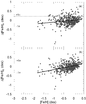
For the second set, there is an agreement between the mean deviations for two calibrations only for the metallicity interval $-1.76<[Fe/H]\leq-1$ dex. The mean deviation of the residuals estimated via $f_{S}$, for the metallicity interval $-0.5<[Fe/H]\leq 0$ dex, is a bit smaller than the ones estimated via $f_{K}$, whereas, for two metallicity intervals, i.e. $-1<[Fe/H]\leq-0.5$ and $0<[Fe/H]\leq+0.4$ dex, the mean deviations corresponding to $f_{K}$ are much smaller than the ones of $f_{S}$. In Fig. 10, the residuals estimated via $f_{K}$ and $f_{S}$ are calibrated to linear equations of the metallicities. However, the inclination of the line for the upper panel (0.10) is less than the one for the lower panel (0.20), indicating that the metallicities estimated by means of the calibration based on metallicity dependent guillotine factors agree better with the original metallicities relative to the other set of estimated metallicities.

We showed that the metallicity dependent guillotine factors provide more accurate metallicities relative to the ones estimated by using the guillotine factors in the literature. This work will be useful for the astronomers who would work with $UBV$ photometry, which has the advantage of being able to be transformed to other systems.

5 Acknowledgments

All the authors are greatful to the anonymous referee whose comments and suggestions improved the paper. S. Karaali is grateful to the Beykent University for financial support. This research has made use of the SIMBAD database, operated at CDS, Strasbourg, France and NASA/IPAC Extragalactic Database (NED) which is operated by the Jet Propulsion Laboratory, California Institute of Technology, under contract with the National Aeronautics and Space Administration.

References

- Ak et al. (2007a) Ak, S., Bilir, S., Karaali, S., Buser, R. 2007a, AN, 328, 169
- Ak et al. (2007b) Ak, S., Bilir, S., Karaali, S., Buser, R., Cabrera-Lavers, A. 2007b, NewA, 12, 605
- Bahcall & Soneira (1980) Bahcall, J. N., Soneira, R. M. 1980, ApJS, 44, 73
- Buser & Kurucz (1978) Buser, R., Kurucz, R. L. 1978, A&A, 70, 555
- Buser & Kurucz (1985) Buser, R., Kurucz, R. L. 1985, Calibration of fundamental stellar quantities; Proceedings of the Symposium, Como, Italy, May 24-29, 1984. Dordrecht, D. Reidel Publishing Co., 513
- Buser & Fenkart (1990) Buser, R., Fenkart, R. P. 1990, A&A, 239, 243
- Buser & Kurucz (1992) Buser, R., Kurucz, R. L. 1992, A&A, 264, 557
- Cameron (1985) Cameron, L. M. 1985, A&A, 152, 250
- Carney (1979) Carney, B. W. 1979, ApJ, 233, 211
- Cayrel de Strobel et al. (2001) Cayrel de Strobel, G., Soubiran, C., Ralite, N. 2001, A&A, 373, 159
- Fuhrmann (2008) Fuhrmann, K. 2008, MNRAS, 384, 173
- Hauck et al. (1990) Hauck, B., Nitschelm, C., Mermilliod, M., Mermilliod, J.-C. 1990A&AS, 85, 989
- Karaali et al. (2003) Karaali, S., Bilir, S., Karataş, Y., Ak, S. 2003, PASA, 20, 165
- Karataş & Schuster (2006) Karataş, Y., Schuster, W. 2006, MNRAS, 371, 1793
- Lejeune et al. (1997) Lejeune, Th., Cuisinier, F., Buser, R. 1997, A&AS, 125, 229
- Luck & Heiter (2006) Luck, R. E., Heiter, U. 2006, AJ, 131, 3069
- Marshall et al. (2006) Marshall D. J., Robin A. C., Reylé C., Schultheis M., Picaud S. 2006, A&A, 453, 635
- Mishenina et al. (2004) Mishenina, T. V., Soubiran, C., Kovtyukh, V. V., Korotin, S. A. 2004, A&A, 418, 551
- Nissen et al. (2002) Nissen, P. E., Primas, F., Asplund, M., Lambert, D. L. 2002, A&A, 390, 235
- Ramirez & Melendez (2005) Ramirez, I., Melendez, J. 2005, ApJ, 626, 446
- Roman (1955) Roman, N. G. 1955, ApJS, 2, 195
- Ryan & Smith (2003) Ryan, S. G., Smith, I. M. 2003, MNRAS, 341, 199
- Sandage & Eggen (1959) Sandage, A., Eggen, O. J. 1959, MNRAS, 119, 278
- Sandage (1969) Sandage, A. 1969, ApJ, 158, 1115
- Santos et al. (2004) Santos, N. C., Israelian, G., Mayor, M. 2004, A&A, 415, 1153
- Schlegel et al. (1998) Schlegel, D. J., Finkbeiner, D. P., Davis, M. 1998, ApJ, 500, 525
- Schwarzschild et al. (1955) Schwarzschild, M., Searle, L., Howard, R. 1955, ApJ, 122, 353
- Soubiran et al. (2010) Soubiran, C., Le Campion, J.-F., Cayrel de Strobel, G., Caillo, A. 2010, A&A, 515, 111
- Sousa et al. (2008) Sousa, S. G., Santos, N. C., Mayor, M., Udry, S., Casagrande, L., Israelian, G., Pepe, F., Queloz, D., Monteiro, M. J. P. F. G. 2008, A&A, 487, 373
- Spite et al. (1996) Spite, M., Francois, P., Nissen, P. E., Spite, F. 1996, A&A, 307, 172
- Strömgren (1966) Strömgren, B. 1966, ARA&A, 4, 433
- Tomkin & Lambert (1999) Tomkin, J., Lambert, D. L. 1999, ApJ, 523, 234
- Trefzger et al. (1995) Trefzger, Ch. F., Pel, J. W., Gabi, S. 1995, A&A, 304, 381
- Valenti & Fischer (2005) Valenti, J. A., Fischer, D. A. 2005, ApJS, 159, 141
- van Leeuwen (2007) van Leeuwen, F. 2007, ASSL, 350
- Vandenberg & Bell (1985) Vandenberg, D. A., Bell, R. A. 1985, ApJS, 58, 561
- Wallerstein & Carlson (1960) Wallerstein, G., Carlson, M. 1960, ApJ, 132, 276
- Wallerstein (1962) Wallerstein, G. 1962, ApJS, 6, 407
- Walraven & Walraven (1960) Walraven, Th., Walraven, J. H. 1960, Bull. Astron. Inst. Netherlands 15, 67
- Wildey et al. (1962) Wildey, R. L., Burbidge, E. M., Sandage, A. R., Burbidge, G. R. 1962, ApJ, 135, 94
- Yaz & Karaali (2010) Yaz, E., Karaali, S. 2010, NewA, 15, 234