Anomalous dissipation and energy cascade in 3D inviscid flows

Abstract.

Adopting the setting for the study of existence and scale locality of the energy cascade in 3D viscous flows in physical space recently introduced by the authors to 3D inviscid flows, it is shown that the anomalous dissipation is – in the case of decaying turbulence – indeed capable of triggering the cascade which then continues ad infinitum, confirming Onsager’s predictions.

1. Introduction

The paper in hand concerns the phenomenon of ‘anomalous dissipation’ and existence of the energy cascade in 3D inviscid incompressible flows described by the 3D Euler equations,

$${\bf{u}}_{t}+({\bf{u}}\cdot\nabla){\bf{u}}=-\nabla p,$$

supplemented with the incompressibility condition $\,\mbox{div}\,{\bf{u}}=0$. The vector field ${\bf{u}}$ represents the velocity of the fluid and the scalar field $p$ the (internal) pressure; the density is set to 1.

It was conjectured by Onsager in 1949 [On49] that “…in three dimensions a mechanism for complete dissipation of all kinetic energy, even without aid of the viscosity, is available.” More precisely, Onsager conjectured that the minimal spatial regularity of a (weak) solution to the 3D Euler equations needed to conserve energy is $\bigl{(}\frac{1}{3}\bigr{)}^{+}$, and that in the case the energy is not conserved, the energy dissipation due to the lack of regularity – the anomalous dissipation – triggers the energy cascade that continues ad infinitum (cf. a summary of Onsager’s published and unpublished contributions to turbulence by Eyink and Sreenivasan [ES06]). In fact, as noticed in [ES06], the following quotation from Onsager’s note to Lin (1945) seems to contain the first use of the word cascade in the theory of turbulence, “The selection rule for the ‘modulation’ factor in each term of (8) suggests a ‘cascade’ mechanism for the process of dissipation, and also furnishes a dynamical basis for an assumption which is usually made on dimensional grounds only”.

There has been a series of mathematical works pertaining $\frac{1}{3}$ minimality (most notably, the papers by Eyink [E94], Constantin, E. and Titi [CET94] and Duchon and Robert [DR00]) culminating with the paper by Cheskidov, Constantin, Friedlander and Shvydkoy [CCFS08] giving a solution to one direction in $\frac{1}{3}$-minimality conjecture, namely, showing that as long as a weak solution to the 3D Euler equations is in the space $L^{3}(0,T;B^{\frac{1}{3}}_{3,c_{0}})$ – $B^{\frac{1}{3}}_{3,c_{0}}$ being a subspace of Besov space $B^{\frac{1}{3}}_{3,\infty}$ in which boundedness over the Littlewood-Paley parameter $q$ is replaced with the zero limit – the energy equality holds. Looking more precisely into local spatiotemporal structure and assuming that the singular set is a smooth manifold, Shvydkoy [Shvy09] presented various spatiotemporal regularity criteria for the energy conservation dimensionally equivalent to the critical one. In addition, a complete solution to Onsager’s $\frac{1}{3}$ minimality in this setting was given for dyadic models (the models in which the original non-local nonlinearity is replaced by a nonlinearity that is local by design) (cf. [CF09]). It may be tempting to think that Onsager critical spatial regularity is also necessary for a weak solution to conserve the energy; however, a family of explicit energy-conserving flows well below Onsager criticality was recently given by Bardos and Titi [BT10] .

On the other hand, to the best of our knowledge, there has been no rigorous mathematical work showing that the anomalous dissipation is indeed capable of triggering the energy cascade.

Various methods of obtaining weak solutions to the Euler equations were introduced in [Sc93, Shn97, Shn00, DLS09, DLS10]. In particular, the construction in [Shn00] and a very recent work [DLS10] yield energy-dissipating weak solutions to the 3D Euler.

Recall that an $L^{3}_{loc}$ (in the space-time) solution ${\bf{u}}=(u^{1},u^{2},u^{3})$ satisfies the local energy inequality if

$$\partial_{t}\frac{1}{2}|{\bf{u}}|^{2}+\,\mbox{div}\,\biggl{(}\Bigl{(}\frac{1}{2}|{\bf{u}}|^{2}+p\Bigr{)}{\bf{u}}\biggr{)}\leq 0$$

in the sense of distributions, i.e., if

(1.1) $$\frac{1}{2}\iint|{\bf{u}}|^{2}\partial_{t}\phi\,d{\bf{x}}\,dt\ +\iint\Bigl{(}\frac{1}{2}|{\bf{u}}|^{2}+p\Bigr{)}{\bf{u}}\cdot\nabla\phi\,d{\bf{x}}\,dt\geq 0$$

for all nonnegative test functions $\phi$. (Note that

$$-\Delta p=\partial_{i}\partial_{j}u^{i}u^{j}$$

and the local elliptic theory imply that – provided ${\bf{u}}$ is in $L^{3}_{loc}$ – all the terms in (1.1) are well-defined.)

Let ${\bf{u}}$ be a weak solution to the 3D Navier-Stokes equations (NSE) or an $L^{3}$ (in the space-time) weak solution to the 3D Euler equations. (One should note that, at present, no general construction of $L^{3}$ weak solutions to the 3D Euler equations exists.) Duchon and Robert [DR00] (in the case of the torus) gave an explicit limit formula for a distribution $D({\bf{u}})$ (in the space-time) measuring anomalous dissipation in the flow; defining $D({\bf{u}})$ by

$$D({\bf{u}})=\lim_{\epsilon\to 0}\frac{1}{4}\int\nabla\phi^{\epsilon}({\bf{y}})\cdot\delta{\bf{u}}|\delta{\bf{u}}|^{2}\,d{\bf{y}}$$

where $\delta{\bf{u}}={\bf{u}}({\bf{x}}+{\bf{y}})-{\bf{u}}({\bf{x}})$ and $\{\phi^{\epsilon}\}$ is a family of standard mollifiers, the following form of the local energy equality holds,

(1.2) $$\partial_{t}\Bigl{(}\frac{1}{2}|{\bf{u}}|^{2}\Bigr{)}+\,\mbox{div}\,\biggl{(}\Bigl{(}\frac{1}{2}|{\bf{u}}|^{2}+p\Bigr{)}{\bf{u}}\biggr{)}-\nu\Delta\frac{1}{2}|{\bf{u}}|^{2}+\nu|\nabla{\bf{u}}|^{2}+D({\bf{u}})=0$$

($\nu=0$ for the Euler). Notice that in the case of the 3D NSE, $D({\bf{u}})\geq 0$ (in the sense of distributions) is equivalent to the local energy inequality; this is satisfied by all ‘suitable weak solutions’ constructed in [Sc77, CKN82], and in fact by any weak solution obtained as a limit of a subsequence of the Leray regularizations. In the case of the 3D Euler, $D({\bf{u}})\geq 0$ – or equivalently, the local energy inequality (1.1) holds – for any $L^{3}$ weak solution obtained as a strong $L^{3}$-limit of weak solutions to the 3D NSE (as the viscosity $\nu$ goes to 0) satisfying the local energy inequality. This motivated Duchon and Robert to call weak solutions to the 3D incompressible fluid equations satisfying $D({\bf{u}})\geq 0$ ‘dissipative’. Any ‘dissipative’ solution to the 3D Euler is also dissipative in the sense of Lions [PLL96]; a detailed proof of this fact can be found in [DLS10], Appendix B. Note that we do not know if globally dissipative solutions constructed in [Shn00, DLS10] are locally dissipative; there may be regions exhibiting local creation of energy. However, at any given spatial scale $R_{0}$, there will be regions exhibiting energy dissipation.

In this paper, we show – via suitable ensemble averaging of the local energy inequality over a region containing (possible) singularities of the 3D Euler equations – that provided the anomalous dissipation in the region is strong enough (with respect to the energy), the energy cascade commences and continues ad infinitum, confirming Onsager’s predictions. In fact, in the case of a spatially isolated singularity – provided the anomalous dissipation is positive, i.e., the strict energy inequality holds on some neighborhood of the singular curve – the cascade condition will hold on any small enough (in the spatial coordinates) neighborhood of the singular curve.

The approach is based on a very recent work [DG10] in which a setting for a rigorous mathematical study of the energy cascade in physical space was introduced. More precisely, the 3D NSE were utilized via ensemble averaging of the local energy inequality over a region of interest with respect to ‘$(K_{1},K_{2})$-covers’ (see below) to establish both existence of the energy cascade and scale locality in decaying turbulence – zero driving force and non-increasing global energy – under a very simple condition plausible in the regions of intense fluid activity (large gradients); namely, that Taylor micro scale is dominated by the integral scale. This furnished the first proof of existence of the energy cascade in 3D viscous flows in physical scales, as well as the only mathematical setting in which both existence of the cascade and locality were obtained directly from the 3D NSE.

For simplicity, assume that the region of interest is ball $B({\bf{0}},R_{0})$ ($R_{0}$ being the integral scale), $B({\bf{0}},2R_{0})$ contained in the global spatial domain, and $0<R\leq R_{0}$. Let $K_{1}$ and $K_{2}$ be two positive integers. A cover $\{B({\bf{x}}_{i},R)\}_{i=1}^{n}$ of $B({\bf{0}},R_{0})$ is a $(K_{1},K_{2})$ cover at scale $R$ if

$$\biggl{(}\frac{R_{0}}{R}\biggr{)}^{3}\leq n\leq K_{1}\biggr{(}\frac{R_{0}}{R}\biggr{)}^{3},$$

and any point ${\bf{x}}$ in $B({\bf{0}},R_{0})$ is covered by at most $K_{2}$ balls $B({\bf{x}}_{i},2R)$; the parameters $K_{1}$ and $K_{2}$ represent global and local maximal multiplicities, respectively.

Remark 1.1.

The $(K_{1},K_{2})$-covers were originally named ’optimal coverings’ [DG10]; here – and elsewhere – we renamed them ‘$(K_{1},K_{2})$-covers‘ to emphasize a key role played by the maximal multiplicities $K_{1}$ and $K_{2}$.

Let $f$ be an a priori sign-varying density corresponding to some physical quantity of interest (e.g., the flux density $-[({\bf{u}}\cdot\nabla){\bf{u}}+\nabla p]\cdot{\bf{u}}$), and consider the arithmetic mean of the quantity per unit mass averaged over the cover elements $B({\bf{x}}_{i},R)$,

$$F_{R}=\frac{1}{n}\sum_{i=1}^{n}\frac{1}{R^{3}}\int_{B({\bf{x}}_{i},2R)}f\,\psi_{i}^{\delta}\,d{\bf{x}},$$

for some $0<\delta\leq 1$ where $\psi_{i}$ are smooth spatial cut-offs associated with the balls $B({\bf{x}}_{i},R)$. The key property of the ensemble averages $F_{R}$ is that $F_{R}\approx\,\mbox{const}\,(R)\$ for all $(K_{1},K_{2})$-covers at scale $R$ indicates there are no significant sign-fluctuations of the density $f$ at scales comparable or greater than $R$. In other words, if there are significant sign-fluctuations at scale $R^{*}$, the averages $F_{R}$ will run over a wide range of values (across, say, an interval $(-M,M)$ for some large $M$) – simply by rearranging and stacking up the cover elements up to the maximal multiplicities – for any $R$ comparable or less than $R^{*}$. Hence, the averages act as a coarse detector of the sign-fluctuations at scale $R$ (of course, the large the multiplicities, the finer detection).

In the case of a signed quantity (e.g., the energy density or the enstrophy density) – for any scale $R$, $0<R\leq R_{0}$ – the averages $F_{R}$ are all comparable to each other and in particular, to the simple average over the spatial integral domain.

Let ${\bf{u}}$ be a weak solution to the 3D Euler equations satisfying the local energy inequality (1.1) (dissipative in the sense of [DR00]). Given $\phi$ – a smooth spatiotemporal cut-off over $(0,2T)\times B({\bf{x}},2R)$ – denote by $\varepsilon_{{\bf{x}},R}$ the anomalous dissipation due to (possible) singularities located in the support of $\phi$

(1.3) $$\varepsilon_{{\bf{x}}_{,}R}=\iint\Bigl{(}\frac{1}{2}|{\bf{u}}|^{2}+p\Bigr{)}{\bf{u}}\cdot\nabla\phi\,d{\bf{y}}\,dt+\frac{1}{2}\iint|{\bf{u}}|^{2}\partial_{t}\phi\,d{\bf{y}}\,dt\ \geq 0,$$

and let $\varepsilon_{0}=\frac{1}{T}\frac{1}{R_{0}^{3}}\varepsilon_{{\bf{0}},R_{0}}$ indicate the spatiotemporal average of the anomalous dissipation due to singularities in $(0,T)\times B({\bf{0}},2R_{0})$. Following the general idea of ensemble averaging with respect to $(K_{1},K_{2})$-covers, consider the spatiotemporal ensemble averages of the local anomalous dissipation quantities $\{\varepsilon_{{\bf{x}}_{i},R}\}$,

(1.4) $$\varepsilon_{R}=\frac{1}{n}\sum\limits_{i=1}^{n}\frac{1}{T}\frac{1}{R^{3}}\varepsilon_{{\bf{x}}_{i},R}.$$

Note that $\varepsilon_{x_{i},R}=\bigl{(}D_{i}({\bf{u}}),\phi_{i}\bigr{)}$ where $D_{i}({\bf{u}})$ is Duchon-Robert distribution $D({\bf{u}})$ measuring anomalous dissipation associated with the ball $B({\bf{x}}_{i},R)$.

A key property exploited in the proof of existence of the energy cascade in the viscous case (cf. [DG10]) was that the ensemble averages of the time-averaged local viscous dissipation quantities per unit mass at any scale $R$, $0<R\leq R_{0}$, were comparable with the spatiotemporal average of the viscous dissipation term associated to the integral domain $B({\bf{0}},R_{0})$; this was simply a consequence of the enstrophy density being non-negative. The following lemma – to be proved in the subsequent section – provides an analogous statement in the realm of anomalous dissipation, and is a key technical ingredient in establishing the cascade in the inviscid case.

Lemma 1.1.

Let $\{B({\bf{x}}_{i},R)\}_{i=1}^{n}$ be a $(K_{1},K_{2})$-cover of $B({\bf{0}},R_{0})$ at scale $R$. Then, there exists a constant $K=K(K_{1},K_{2})>1$ such that

$$\frac{1}{K}\varepsilon_{0}\leq\varepsilon_{R}\leq K\varepsilon_{0},$$

for any $R$, $0<R\leq R_{0}$.

Remark 1.2.

As a matter of fact, the proof of the lemma can be easily modified to show that the analogous property holds for any non-negative distribution; in light of this observation, the statement of the lemma is simply a consequence of the non-negativity of Duchon-Robert distribution $D({\bf{u}})$.

In the viscous case (3D NSE), the term $\iint|{\bf{u}}|^{2}\nu\Delta\phi\,d{\bf{x}}\,dt\,$ in the local energy inequality furnished the breaking mechanism restricting the inertial range (via the estimate on $\Delta\phi$ with respect to the spatial scale – for details see [DG10]); in the inviscid case, once it starts – provided that $\varepsilon_{0}$ is strong enough compared to the spatiotemporal average of the energy associated with $B({\bf{0}},R_{0})$ – the cascade will continue indefinitely (as expected).

Assuming certain geometric properties of the singular set leads to improved results. As an illustration, we show that in the case of a spatially isolated singularity (the singular set being a curve ${\bf{c}}={\bf{c}}(t)$) – provided the strict energy inequality holds on some neighborhood of the singular curve – the anomalous dissipation will in fact dominate the corresponding energy on any small enough (in spatial directions) neighborhood of the singular curve, triggering the cascade. The reason behind this phenomenon is that – in the case of a spatially isolated singularity – the anomalous dissipation over any family of nested tubular neighborhoods containing the singular curve is constant. Let us note that a natural Onsager critical space here is $(L^{3}_{t}L^{4.5}_{{\bf{x}}})_{loc}$ (cf. [Shvy09]); hence, a class of weak solutions compatible with existence of the energy cascade in this setting is $(L^{3}_{t}L^{\alpha}_{{\bf{x}}})_{loc},\,3\leq\alpha<4.5$.

Scale locality of the cascade manifests in several ways analogous to the viscous case (cf. [DG10]). We present locality of the ensemble averages of the time-averaged fluxes at spatial scale $R$. In particular, considering the dyadic case – $r=2^{k}R$ ($k$ an integer) – both ultraviolet and infrared locality propagate exponentially in $k$ as predicted by turbulence phenomenology.

2. Localized energy and flux; anomalous dissipation and ensemble averages

Let ${\bf{u}}$ be a weak solution to the 3D Euler equations satisfying the local energy inequality on a spatiotemporal domain $\Omega\times(0,2T)$ (for simplicity, assume that $\Omega$ contains the origin), and let $R_{0}>0$ be such that $B({\bf{0}},2R_{0})$ is contained in $\Omega$; $B({\bf{0}},R_{0})$ is our region of interest and $R_{0}$ the integral scale in the problem. Choose $\psi_{0}\in\mathcal{D}(B({\bf{0}},2R_{0}))$ satisfying

(2.1) $$0\leq\psi_{0}\leq 1,\quad\psi_{0}=1\ \mbox{on}\ B({\bf{0}},R_{0})\;.$$

For $T>0$, ${\bf{x}}_{0}\in B({\bf{0}},R_{0})$ and $0<R\leq R_{0}$ define $\phi=\phi_{{\bf{x}}_{0},T,R}(t,{\bf{x}})=\eta(t)\psi({\bf{x}})$ to be used in the local energy inequality (1.1) where $\eta=\eta_{T}(t)$ and $\psi=\psi_{{\bf{x}}_{0},R}({\bf{x}})$ satisfy the following conditions,

(2.2) $$\eta\in\mathcal{D}(0,2T),\quad 0\leq\eta\leq 1,\quad\eta=1\ \mbox{on}\ (T/4,5T/4),\quad\frac{|\eta^{\prime}|}{\eta^{\delta}}\leq\frac{C_{0}}{T}\;$$

for some $0<\delta\leq 1$;

if $B({\bf{x}}_{0},R)\subset B({\bf{0}},R_{0})$, then $\psi\in\mathcal{D}(B({\bf{x}}_{0},2R))$ with $0\leq\psi\leq\psi_{0},\ \psi=1$ on $B({\bf{x}}_{0},R)$,

and if $B({\bf{x}}_{0},R)\not\subset B({\bf{0}},R_{0})$, then $\psi\in\mathcal{D}(B({\bf{0}},2R_{0}))$ with $0\leq\psi\leq\psi_{0},\ \psi=1$ on $B({\bf{x}}_{0},R)\cap B({\bf{0}},R_{0})$ satisfying the following:

$\psi=\psi_{0}$ on the part of the cone in ${\mathbb{R}^{3}}$ centered at zero and passing through $S({\bf{0}},R_{0})\cap B({\bf{x}}_{0},R)$ between $S({\bf{0}},R_{0})$ and $S({\bf{0}},2R_{0})$, and $\psi=0$ on $B({\bf{0}},R_{0})\setminus B({\bf{x}}_{0},2R)$ and outside the part of the cone in ${\mathbb{R}^{3}}$ centered at zero and passing through $S({\bf{0}},R_{0})\cap B({\bf{x}}_{0},2R)$ between $S({\bf{0}},R_{0})$ and $S({\bf{0}},2R_{0})$.

Figure 1 illustrates the definition of $\psi$ in the case $B({\bf{x}}_{0},R)$ is not entirely contained in $B({\bf{0}},R_{0})$.

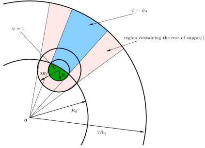
Figure 1. Regions of supp$(\psi)$ in the case $B({\bf{x}}_{0},R)\not\subset B({\bf{0}},R_{0})$, cross-section.

Note that in contrast to the Navier-Stokes case (cf. [DG10]), we do not make growth assumptions on derivatives of $\psi$. As we shall see later, only the time derivatives of the test functions will matter in the cascade formation.

In the case ${\bf{x}}_{0}={\bf{0}}$ and $R=R_{0}$ set

(2.3) $$\phi_{0}(t,{\bf{x}})=\eta(t)\psi_{0}({\bf{x}}).$$

Let ${\bf{x}}_{0}\in B({\bf{0}},R_{0})$ and $0<R\leq R_{0}$. Define localized energy ${\mathsf{e}}$ at time $t$ associated with $B({\bf{x}}_{0},R)$ by

(2.4) $${\mathsf{e}}_{{\bf{x}}_{0},R}(t)=\int\frac{1}{2}|{\bf{u}}|^{2}\phi^{\delta}\,d{\bf{x}}\;.$$

A total inward flux – (kinetic) energy plus pressure – through the boundary of a region $D$ is given by

$$-\int\limits_{\partial D}\biggl{(}\frac{1}{2}|{\bf{u}}|^{2}+p\biggr{)}{\bf{u}}\cdot{\bf{n}}\,ds\,=\,-\int\limits_{D}\Bigl{(}({\bf{u}}\cdot\nabla){\bf{u}}+\nabla p\Bigr{)}\cdot{\bf{u}}\,d{\bf{x}}$$

where ${\bf{n}}$ is an outward normal. Considering the Euler equations localized to $B({\bf{x}}_{0},2R)$ – and utilizing $\,\mbox{div}\,{\bf{u}}=0$ – leads to a localized flux,

(2.5) $$\Phi_{{\bf{x}}_{0},R}(t)=\int\biggl{(}\frac{1}{2}|{\bf{u}}|^{2}+p\biggr{)}{\bf{u}}\cdot\nabla\phi\,d{\bf{x}}=-\int\Bigl{(}({\bf{u}}\cdot\nabla){\bf{u}}+\nabla p\Bigr{)}\cdot{\bf{u}}\,\phi\,d{\bf{x}}.$$

Since $\psi$ can be constructed such that $\nabla\phi=\eta\,\nabla\psi$ is oriented along the radial directions of $B({\bf{x}}_{0},2R)$ toward the center of the ball, $\Phi_{{\bf{x}}_{0},R}$ represents the total flux into $B({\bf{x}}_{0},R)$ through the layer between the spheres $S({\bf{x}}_{0},2R)$ and $S({\bf{x}}_{0},R)$ ($\nabla\phi\equiv 0$ on $B({\bf{x}}_{0},R)$). (In the case of the boundary elements, $\psi$ is almost radial and $\nabla\psi$ still points inward.)

A more dynamic physical significance of the sign of $\Phi_{{\bf{x}}_{0},R}$ can be seen from the equations; for the sake of a more concise interpretation of the local flux term $\Phi_{{\bf{x}}_{0},R}$, let us for a moment assume smoothness. Then, multiplying the Euler equations by $\psi{\bf{u}}$ and integrating over $B({\bf{x}}_{0},2R)$ leads to

(2.6) $$\frac{d}{dt}\int\frac{1}{2}|{\bf{u}}|^{2}\psi\,d{\bf{x}}=\Phi_{{\bf{x}}_{0},R}.$$

Plainly, the positivity of $\Phi_{{\bf{x}}_{0},R}$ implies the increase of the kinetic energy around the point ${\bf{x}}_{0}$ at scale $R$.

The key question is what can we say about the transfer of the kinetic energy around the point ${\bf{x}}_{0}$ at scale $R$, i.e., the total exchange between the kinetic energy associated with the ball $B({\bf{x}}_{0},R)$ and the kinetic energy in the complement of the ball $B({\bf{x}}_{0},2R)$. In general, not much – one can envision a variety of scenarios. However, in physical situations where the kinetic energy on the global spatial domain $\Omega$ is non-increasing (here, we are concerned with the case of decaying turbulence, setting the driving force to zero), the positivity of $\Phi_{{\bf{x}}_{0},R}$ implies the transfer of the kinetic energy around the point ${\bf{x}}_{0}$ – from larger scales – simply because the local kinetic energy is increasing while the global kinetic energy is non-increasing resulting in decrease of the kinetic energy in the complement.

Henceforth, following the discussion in the preceding paragraphs – in the setting of decaying turbulence (zero driving force, non-increasing global energy) – the positivity and the negativity of $\Phi_{{\bf{x}}_{0},R}$ will be interpreted as transfer of kinetic energy around the point ${\bf{x}}_{0}$ at scale $R$ toward smaller scales and transfer of kinetic energy around the point ${\bf{x}}_{0}$ at scale $R$ toward larger scales, respectively.

As in Introduction, denote by $\varepsilon_{{\bf{x}}_{0},R}$ the anomalous dissipation of energy due to (possible) singularities inside $\,\mbox{supp}\,(\phi)$,

(2.7) $$\varepsilon_{{\bf{x}}_{0},R}=\iint\frac{1}{2}|{\bf{u}}|^{2}\partial_{t}\phi\,d{\bf{x}}\,dt+\iint\Bigl{(}\frac{1}{2}|{\bf{u}}|^{2}+p\Bigr{)}{\bf{u}}\cdot\nabla\phi\,d{\bf{x}}\,dt\geq 0\;.$$

For a physical quantity $\Theta_{{\bf{x}},R}(t)$, $t\in(0,2T)$ and a cover $\{B({\bf{x}}_{i},R)\}_{i=1,n}$ of $B({\bf{0}},R_{0})$, consider the time average of the ensemble-averaged local quantities $\Theta_{{\bf{x}}_{i},R}$ per unit mass,

(2.8) $$\langle\Theta\rangle_{R}=\frac{1}{T}\int\frac{1}{n}\sum\limits_{i=1}^{n}\frac{1}{R^{3}}\Theta_{{\bf{x}}_{i},R}(t)\,dt\;.$$

Set

(2.9) $${\mathsf{e}}_{R}=\langle{\mathsf{e}}_{{\bf{x}},R}(t)\rangle_{R}\;$$

and

(2.10) $$\Phi_{R}=\langle\Phi_{{\bf{x}},R}(t)\rangle_{R}\;;$$

the averaged energy and inward-directed flux, respectively.

In addition, consider the ensemble-averaged local anomalous dissipation quantities $\varepsilon_{{\bf{x}}_{i},R}$ – per unit time and per unit mass –

(2.11) $$\varepsilon_{R}=\frac{1}{n}\sum\limits_{i=1}^{n}\frac{1}{T}\frac{1}{R^{3}}\varepsilon_{{\bf{x}}_{i},R}\;.$$

Finally, introduce the spatiotemporal average of the energy associated to $B({\bf{0}},2R_{0})\times(0,2T)$,

(2.12) $${\mathsf{e}}_{0}=\frac{1}{T}\int\frac{1}{R_{0}^{3}}{\mathsf{e}}_{{\bf{0}},R_{0}}(t)\,dt=\frac{1}{T}\frac{1}{R_{0}^{3}}\iint\frac{1}{2}|{\bf{u}}|^{2}\phi_{0}^{\delta}\,d{\bf{x}}\,dt\;$$

and the spatiotemporal average of the anomalous dissipation on $(0,2T)\times B({\bf{x}}_{0},2R)$,

(2.13) $${\varepsilon_{0}}=\frac{1}{T}\frac{1}{R_{0}^{3}}\varepsilon_{{\bf{0}},R_{0}}=\frac{1}{T}\frac{1}{R_{0}^{3}}\iint\frac{1}{2}\Bigl{(}|{\bf{u}}|^{2}\partial_{t}\phi_{0}+(|{\bf{u}}|^{2}+2p){\bf{u}}\cdot\nabla\phi_{0}\Bigr{)}\,d{\bf{x}}\,dt\;$$

with $\phi_{0}$ defined in (2.3), and define (anomalous) Taylor length scale associated with $B({\bf{0}},R_{0})$ by

(2.14) $$\tau_{0}=\left(\frac{R_{0}^{2}}{T}\frac{{\mathsf{e}}_{0}}{\varepsilon_{0}}\right)^{1/2}\;.$$

Henceforth, all the averages $\langle\cdot\rangle_{R}$ are taken with respect to $(K_{1},K_{2})$-covers at scale $R$.

The following lemma will be a key technical ingredient in establishing the energy cascade in the next section.

Lemma 2.1.

Let $\{B({\bf{x}}_{i},R)\}_{i=1,n}$ be a $(K_{1},K_{2})$-cover of $B({\bf{0}},R_{0})$ at scale $R$. Then

(2.15) $${K_{1}}\varepsilon_{0}\leq\varepsilon_{R}\leq K\varepsilon_{0}\;$$

where $K>0$ is a constant depending only on $K_{2}$ and dimension of the space (in ${\mathbb{R}^{3}}$ , one can choose $K=8^{3}K_{2}$).

Proof.

Let $\phi_{i}=\phi_{{\bf{x}}_{i},R}$ be a smooth cut-off function associated with $B({\bf{x}}_{i},R)$ as described in (2.2).

To prove the first inequality in (2.15), note that $\tilde{\phi}=\sum_{i}\phi_{i}-\phi_{0}\geq 0$, and so the local energy inequality (1.1) written for $\tilde{\phi}$,

$$0\leq\iint\frac{1}{2}\left[(|{\bf{u}}|^{2}+2p){\bf{u}}\cdot\nabla(\sum_{i}\phi_{i}-\phi_{0})+|{\bf{u}}|^{2}\partial_{t}(\sum_{i}\phi_{i}-\phi_{0})\right]\,d{\bf{x}}\,dt\;,$$

implies

$$\varepsilon_{0} =\frac{1}{T}\frac{1}{R_{0}^{3}}\iint\frac{1}{2}\left[|{\bf{u}}|^{2}\partial_{t}\phi_{0}+(|{\bf{u}}|^{2}+2p){\bf{u}}\cdot\nabla\phi_{0}\right]\,d{\bf{x}}\,dt$$

$$\leq\frac{1}{T}\frac{1}{R_{0}^{3}}\iint\frac{1}{2}\left[|{\bf{u}}|^{2}\partial_{t}\Bigl{(}\sum_{i}\phi_{i}\Bigr{)}+(|{\bf{u}}|^{2}+2p){\bf{u}}\cdot\nabla(\sum_{i}\phi_{i})\right]\,d{\bf{x}}\,dt$$

$$\leq\frac{1}{K_{1}}\frac{1}{T}\frac{1}{R^{3}}\frac{1}{n}\sum\limits_{i}\iint\frac{1}{2}\left[|{\bf{u}}|^{2}\partial_{t}\phi_{i}+(|{\bf{u}}|^{2}+2p){\bf{u}}\cdot\nabla\phi_{i}\right]\,d{\bf{x}}\,dt=\frac{1}{K_{1}}\varepsilon_{R}\;,$$

where we used the following consequence of the definition of a $(K_{1},K_{2})$-cover,

$$\frac{1}{R_{0}^{3}}\leq\frac{1}{K_{1}}\frac{1}{R^{3}}\frac{1}{n}\,.$$

To prove the second inequality in (2.15), let $\{{\bf{x}}_{i_{j}}\}$ be a subset of $\{{\bf{x}}_{i}\}_{i=1,n}$ such that interiors of the balls $B({\bf{x}}_{i_{j}},2R)$ are pairwise disjoint. Using (2.7), we obtain

(2.16) $$TR_{0}^{3}\,\varepsilon_{0}= \iint\left[(\frac{1}{2}|{\bf{u}}|^{2}+p){\bf{u}}\cdot\nabla\phi_{0}+\frac{1}{2}|{\bf{u}}|^{2}\partial_{t}\phi_{0}\right]\,d{\bf{x}}\,dt\;$$

and

(2.17) $$\sum\limits_{j}\varepsilon_{{\bf{x}}_{i_{j}},R}= \iint\left[(\frac{1}{2}|{\bf{u}}|^{2}+p){\bf{u}}\cdot\nabla(\sum\limits_{j}\phi_{i_{j}})+\frac{1}{2}|{\bf{u}}|^{2}\partial_{t}(\sum\limits_{j}\phi_{i_{j}})\right]\,d{\bf{x}}dt\,.$$

In this scenario

$$\tilde{\phi}=\phi_{0}-\sum\limits_{j}\phi_{i_{j}}\geq 0\;;$$

hence, by the local energy inequality (1.1),

(2.18) $$0\leq \iint(\frac{1}{2}|{\bf{u}}|^{2}+p){\bf{u}}\cdot\nabla\tilde{\phi}\,d{\bf{x}}\,dt+\frac{1}{2}\iint|{\bf{u}}|^{2}\partial_{t}\tilde{\phi}\,d{\bf{x}}\,dt\;.$$

If we add relations (2.17) and (2.18) and then subtract (2.16) we obtain

(2.19) $$\sum\limits_{j}\varepsilon_{{\bf{x}}_{i_{j}},R}\leq TR_{0}^{3}\,\varepsilon_{0}\;.$$

Let $\mathcal{L}$ be a cubic lattice inside $B({\bf{0}},R_{0})$ with the points situated at the vertices of cubes of side $R/2$. (Note that this lattice can be chosen such that the number of points in it is between $2^{3}(R_{0}/R)^{3}$ and $(4\pi/3)2^{3}(R_{0}/R)^{3}$.)

Since the cover $\{B({\bf{x}}_{i},R)\}$ is a $(K_{1},K_{2})$-cover, each point in $\mathcal{L}$ is contained in at most $K_{2}$ balls. Moreover, any ball in the cover will contain at least one point from the lattice.

If $\mathcal{L}^{\prime}$ is sub-lattice of $\mathcal{L}$ with points at vertices of cubes of side $4R$, then the interiors of balls of radius $2R$ containing different points of $\mathcal{L}^{\prime}$ are pairwise disjoint, and thus if we denote by $B({\bf{x}}_{i_{p}},R)$ a ball from the cover $\{B({\bf{x}}_{i},R)\}$ containing the point $p\in\mathcal{L}^{\prime}$, by (2.18),

$$\sum\limits_{p\in\mathcal{L}^{\prime}}\varepsilon_{{\bf{x}}_{i_{p}},R}\leq TR_{0}^{3}\,\varepsilon_{0}\;.$$

Note that for each point $p\in\mathcal{L}^{\prime}$ there are at most $K_{2}$ choices for $B({\bf{x}}_{i_{p}},R)$. So

$$\sum\limits_{i:B({\bf{x}}_{i},R)\cap\mathcal{L}^{\prime}\not=\emptyset}\varepsilon_{{\bf{x}}_{i},R}\leq K_{2}TR_{0}^{3}\,\varepsilon_{0}\;.$$

Clearly $\mathcal{L}$ can be written as a union of $8^{3}=256$ sub-lattices $\mathcal{L}^{\prime}_{k}$, $k=1,\dots,256$, each $\mathcal{L}^{\prime}_{k}$ having the same properties as $\mathcal{L}^{\prime}$. Thus,

$$\sum\limits_{i=1}^{n}\varepsilon_{{\bf{x}}_{i},R}\leq 8^{3}K_{2}TR_{0}^{3}\,\varepsilon_{0}\;.$$

Consequently,

$$\varepsilon_{R}=\frac{1}{T}\frac{1}{R^{3}}\frac{1}{n}\sum\limits_{i=1}^{n}\varepsilon_{{\bf{x}}_{i},R}\leq 8^{3}K_{2}\left(\frac{R_{0}}{R}\right)^{3}\frac{1}{n}\,\varepsilon_{0}\leq 8^{3}K_{2}\,\varepsilon_{0}\;.$$

∎

Remark 2.1.

Note that the defect in the local energy inequality can be interpreted either as the anomalous dissipation or as the anomalous flux. The second interpretation was adopted – in the context of 3D viscous flows – in [DG10] which contains a proof of the upper bound in the lemma interpreted as an upper bound on the averaged anomalous fluxes.

3. Energy Cascade

Let $\{B({\bf{x}}_{i},R)\}_{i=1,n}$ be a $(K_{1},K_{2})$-cover of $B({\bf{0}},R_{0})$ at scale $R$. Definitions of $\varepsilon_{R}$ and $\Phi_{R}$ – (2.11) and (2.10) – imply

(3.1) $$\Phi_{R}=\varepsilon_{R}-\frac{1}{n}\sum\limits_{i=1}^{n}\frac{1}{T}\frac{1}{R^{3}}\iint\frac{1}{2}|{\bf{u}}|^{2}\partial_{t}\phi_{i}\,d{\bf{x}}\,dt\;$$

where $\phi_{i}=\eta\psi_{i}$ and $\psi_{i}$ is the spatial cut-off on $B({\bf{x}}_{i},2R)$ satisfying (2.2).

(3.2) $$|(\phi_{i})_{t}|=|\eta_{t}\psi_{i}|\leq C_{0}\frac{1}{T}\eta^{\delta}\psi_{i}\leq\frac{C_{0}}{T}\phi_{i}^{\delta}\,;$$

hence,

$$\Phi_{R}\geq\varepsilon_{R}-\frac{C_{0}}{T}\,{\mathsf{e}}_{R}.$$

The definition of $(K_{1},K_{2})$-covers at scale $R$ and the design of $\psi_{i}$ paired with (2.9) imply

(3.3) $${\mathsf{e}}_{R}\leq{K_{2}}{\mathsf{e}}_{0}\;,$$

while Lemma 2.1 states

(3.4) $$\varepsilon_{R}\geq{K_{1}}\varepsilon_{0}.$$

Consequently,

(3.5) $$\Phi_{R}\geq{K_{1}}\varepsilon_{0}-\frac{C_{0}K_{2}}{T}\,{\mathsf{e}}_{0}\geq K_{1}\varepsilon_{0}\,\left(1-c_{1}\frac{\tau_{0}^{2}}{R_{0}^{2}}\right)$$

with $c_{1}=C_{0}K_{2}/K_{1}$.

Suppose that

(3.6) $$\tau_{0}<\frac{\gamma}{c_{1}^{1/2}}R_{0}$$

for some $0<\gamma<1$. Then, for any $R\leq R_{0}$, (3.5) yields

(3.7) $$\Phi_{R}\geq{K_{1}}(1-\gamma^{2})\varepsilon_{0}=c_{0,\gamma}\varepsilon_{0}\;$$

where

(3.8) $$c_{0,\gamma}={K_{1}}(1-\gamma^{2})\;.$$

To obtain an upper bound on the averaged flux, we utilize the estimates (3.2) and (3.3) in the identity (3.1) again, this time together with the upper bound in Lemma 2.1 to obtain

$$\Phi_{R}\leq\varepsilon_{R}+\frac{C_{0}}{T_{0}}{\mathsf{e}}_{R}\leq K\varepsilon_{0}+C_{0}K_{2}\frac{1}{T}\,{\mathsf{e}}_{0}.$$

If the condition (3.6) holds for some $0<\gamma<1$, then it follows that for any $R\leq R_{0}$,

(3.9) $$\Phi_{R}\leq K\varepsilon_{0}+\frac{C_{0}K_{2}\gamma^{2}}{c_{1}}\varepsilon_{0}\leq c_{1,\gamma}\varepsilon_{0}\;$$

where

(3.10) $$c_{1,\gamma}=K\left[1+\frac{C_{0}K_{2}\gamma^{2}}{c_{1}K}\right]=K\left[1+\frac{K_{1}}{K}\gamma^{2}\right]\;.$$

Thus we have proved the following.

Theorem 3.1.

Assume that for some $0<\gamma<1$

(3.11) $$\tau_{0}<{\gamma}c\,R_{0}\;,$$

where

(3.12) $$c=\sqrt{\frac{K_{1}}{C_{0}K_{2}}}\;.$$

Then, for all $R$,

(3.13) $$0<R\leq R_{0},$$

the averaged energy flux $\Phi_{R}$ satisfies

(3.14) $$c_{0,\gamma}\varepsilon_{0}\leq\Phi_{R}\leq c_{1,\gamma}\varepsilon_{0}\;$$

where

(3.15) $$c_{0,\gamma}=K_{1}({1-\gamma^{2}})\,,\quad c_{1,\gamma}=K\left[1+\frac{K_{1}}{K}\gamma^{2}\right]\;,$$

and the average $\langle\cdot\rangle_{R}$ is computed over a time interval $(0,2T)$ and determined by a $(K_{1},K_{2})$-cover of $B({\bf{0}},R_{0})$ at scale $R$.

As already noted in the previous section – in the case the global energy is non-increasing – the positivity of the local flux $\Phi_{{\bf{x}}_{i},R}$ implies transfer of the kinetic energy around the point ${\bf{x}}_{i}$ at scale $R$ from larger to smaller scales. Since we assume no spatial homogeneity, the positivity of the flux expressed in the theorem holds only in the averaged sense over the integral domain. This may cause some uneasiness, as the transfer of the kinetic energy around the point ${\bf{x}}_{i}$ at scale $R$ is, in general, not necessarily dominantly local; this is due to the fact that the pressure – in terms of the velocity of the flow – is given by a non-local operator. In order to ensure existence of a bona fide (kinetic) energy cascade, we need locality in the sense of turbulence phenomenology, i.e., for the averaged flux at the given scale to be well-correlated only with the averaged fluxes at nearby scales, throughout the inertial range. This is in fact true, and is a simple consequence of the universality of the averaged fluxes per unit mass $\Phi_{R}$ displayed in Theorem 3.1. More precisely, denoting by $\widetilde{\Phi}_{R}$ the time-averaged ensemble average of the local fluxes $\Phi_{{\bf{x}}_{i},R}$,

$$\widetilde{\Phi}_{R}=\frac{1}{T}\int\frac{1}{n}\sum\limits_{i=1}^{n}\Phi_{{\bf{x}}_{i},R}(t)\,dt=R^{3}\Phi_{R},$$

the following holds.

Theorem 3.2.

Let $R$ and $r$ be two spatial scales within the inertial range obtained in Theorem 3.1. Then,

$$\frac{c_{0,\gamma}}{c_{1,\gamma}}\biggl{(}\frac{R}{r}\biggr{)}^{3}\leq\frac{\widetilde{\Phi}_{R}}{\widetilde{\Phi}_{r}}\leq\frac{c_{1,\gamma}}{c_{0,\gamma}}\biggl{(}\frac{R}{r}\biggr{)}^{3}$$

where the constants are the same as in Theorem 3.1.

Remark 3.1.

In particular, in the dyadic case – $r=2^{k}R$ – both the infrared and the ultraviolet locality propagate exponentially in the dyadic parameter $k$. More precisely,

$$\frac{c_{0,\gamma}}{c_{1,\gamma}}2^{-3k}\leq\frac{\widetilde{\Phi}_{R}}{\widetilde{\Phi}_{2^{k}R}}\leq\frac{c_{1,\gamma}}{c_{0,\gamma}}2^{-3k}.$$

Note that the ultraviolet locality in the inviscid case is more pronounced than in the viscous case as the cascade here continues ad infinitum ($r\to 0\ \Leftrightarrow k\to-\infty$).

Remark 3.2.

In the language of turbulence, the condition (3.11) simply reads that the (anomalous) Taylor micro-scale computed over the domain in view is smaller than the integral scale (diameter of the domain).

Remark 3.3.

Unlike in the Navier-Stokes case (cf. [DG10]), we do not impose an explicit constraint on the length of the time interval $T$. Implicitly, $T$ is a part of cascade condition (3.11) through the definition of Taylor scale $\tau_{0}$ (2.14).

4. Cascade near spatially isolated singularity

Assuming certain geometric structure of the singular set leads to improved results on existence of the energy cascade in 3D inviscid flows. In particular – in the case of a spatially isolated singularity (the singular set being a curve ${\bf{c}}={\bf{c}}(t)$) – it is enough to assume that the strict energy inequality holds on some neighborhood of the singular curve. For simplicity, we present the proof in the case the curve is a line segment; the proof easily generalizes to the case of a smooth curve.

The following lemma states that the anomalous dissipation is constant on tubular neighborhoods of the singular line segment.

Lemma 4.1.

Let $0<R_{1}<R_{2},T>0$, and let ${\bf{u}}$ be weak solution to the 3D Euler equations on $B({\bf{0}},2R_{2})\times(0,2T)$ satisfying the local energy inequality, smooth on $\Bigl{(}B({\bf{0}},2R_{2})\setminus\{{\bf{0}}\}\Bigr{)}\times(0,2T)$. Then

$$\varepsilon_{{\bf{0}},R_{1}}=\varepsilon_{{\bf{0}},R_{2}}.$$

Proof.

Let $\phi_{1}$ and $\phi_{2}$ be test functions on $B({\bf{0}},2R_{1})$ and $B({\bf{0}},2R_{2})$, equal to 1 on $B({\bf{0}},R_{1})$ and $B({\bf{0}},R_{2})$, respectively. Since ${\bf{u}}$ is smooth on the support of $\phi_{2}-\phi_{1}$, integration by parts yields

$$\iint\Bigl{(}\frac{1}{2}|{\bf{u}}|^{2}+p\Bigr{)}{\bf{u}}\cdot\nabla(\phi_{2}-\phi_{1})\,d{\bf{x}}\,dt+\frac{1}{2}\iint|{\bf{u}}|^{2}\partial_{t}(\phi_{2}-\phi_{1})\,d{\bf{x}}\,dt\ =0;$$

hence, $\varepsilon_{{\bf{0}},R_{1}}=\varepsilon_{{\bf{0}},R_{2}}$. ∎

The general theorem on existence of 3D inviscid energy cascade – Theorem 3.1. – paired with the above lemma yields the following result on existence of the cascade in the neighborhood of a singular line.

Theorem 4.1.

Let $R,T>0$, and let ${\bf{u}}$ be weak solution to the 3D Euler equations on $B({\bf{0}},2R)\times(0,2T)$ satisfying the local energy inequality, smooth on $\Bigl{(}B({\bf{0}},2R)\setminus\{{\bf{0}}\}\Bigr{)}\times(0,2T)$. Assume that the strict energy inequality holds on $B({\bf{0}},2R^{*})\times(0,2T)$ for some $R^{*}$, $0<R^{*}\leq R$, i.e., $\varepsilon_{{\bf{0}},R^{*}}>0$. Then, there exists $R_{0}^{*}$, $0<R_{0}^{*}\leq R$ such that the cascade condition (3.11), $\tau_{0}<{\gamma}c\,R_{0}$, holds for any $R_{0}$, $0<R_{0}\leq R_{0}^{*}$.

Proof.

Note that the cascade condition holds on $B({\bf{0}},2R_{0})\times(0,2T)$ for some $R_{0}$, $0<R_{0}\leq R$ if and only if

$$\iint\frac{1}{2}|{\bf{u}}|^{2}\phi_{0}<\gamma^{2}c^{2}T\varepsilon_{{\bf{0}},R_{0}}.$$

However, by the above lemma,

$$\varepsilon_{{\bf{0}},R_{0}}=\varepsilon_{{\bf{0}},R^{*}}>0.$$

Since ${\bf{u}}$ is a weak solution with the locally finite energy, the condition will hold for all sufficiently small $R_{0}$. ∎

As already noted in Introduction, a natural Onsager critical space in this setting is $(L^{3}_{t}L^{4.5}_{{\bf{x}}})_{loc}$ (cf. [Shvy09]); hence, a natural class of weak solutions to be considered here is $(L^{3}_{t}L^{\alpha}_{{\bf{x}}})_{loc},\,3\leq\alpha<4.5$.

References

- [On49] L. Onsager, Nuovo Cimento (9), 6 (Supplemento, 2 (Convegno Internazionale di Meccanica Statistica)), 279 (1949).
- [Sc77] V. Scheffer Hausdorff measure and the Navier-Stokes equations. Comm. Math. Phys. 55 97 (1977).
- [CKN82] L. Caffarelli, R. Kohn and L. Nirenberg Partial regularity of suitable weak solutions of the Navier-Stokes equations. Comm. Pure Appl. Math 35, 771 (1982).
- [Sc93] V. Scheffer An inviscid flow with compact support in space-time. J. Geom. Anal. 1993, 343 (1993).
- [E94] G. Eyink Energy dissipation without viscosity in ideal hydrodynamics. I. Fourier analysis and local energy transfer. Phys. D 78, 222 (1994).
- [CET94] P. Constantin, W. E and E. Titi Onsager’s conjecture on the energy conservation for solutions of Euler’s equation. Comm. Math. Phys. (165), 207 (1994).
- [Fr95] U. Frisch, Turbulence. Cambridge University Press, 1995. The legacy of A.N. Kolmogorov.
- [PLL96] P.-L. Lions, Mathematical Topics in Fluid Mechanics vol 1 Incompressible Models. Oxford: Clarendon, 1996.
- [Shn97] A. Shnirelman On the nonuniqueness of weak solution of the Euler equation. Comm. Pure Appl. Math. 50, 1261 (1997).
- [Shn00] A. Shnirelman Weak solutions with decreasing energy of incompressible Euler equations. Comm. Math. Phys. 210, 541 (2000).
- [DR00] J. Duchon and R. Robert Inertial energy dissipation for weak solutions of incompressible Euler and Navier-Stokes equations. Nonlinearity 13, 249 (2000).
- [ES06] G. Eyink and K. Sreenivasan Onsager and the theory of hydrodynamic turbulence. Rev. Mod. Phy. 78, 87 (2006)
- [CCFS08] A. Cheskidov, P. Constantin, S. Friedlander and R. Shvydkoy Energy conservation and Onsager’s conjecture for the Euler equations. Nonlinearity 21, 1233 (2008).
- [CF09] A. Cheskidov and S. Friedlander The vanishing viscosity limit for a dyadic model. Phys. D 238, 783 (2009).
- [Shvy09] R. Shvydkoy On the energy of inviscid singular flows. J. Math. Anal. Appl. 349, 583 (2009).
- [DLS09] C. De Lellis and L. Szekelyhidi Jr, The Euler equations as a differential inclusion. Ann. Math. (2) 170, 1417 (2009).
- [DLS10] C. De Lellis and L. Szekelyhidi Jr On admissibility criteria for weak solutions of the Euler equations. Arch. Rational Mech. Anal. 195, 225 (2010).
- [BT10] C. Bardos and E. Titi Loss of smoothness and energy conserving rough weak solutions for the Euler equations. Discrete Cont. Dynamical Sysytems S 3, 185 (2010).
- [DG10] R. Dascaliuc and Z. Grujić Energy cascades and flux locality in physical scales of the 3D NSE. Comm. Math. Phys. 305, 199 (2011).