Topology,
and (in)stability
of non-Abelian monopoles

Abstract

The stability problem of non-Abelian monopoles with respect to “Brandt–Neri–Coleman type” variations reduces to that of a pure gauge theory on the two-sphere. Each topological sector admits exactly one stable monopole charge, and each unstable monopole admits $\displaystyle{2\sum\left(2|q|-1\right)}$ negative modes, where the sum goes over the negative eigenvalues $q$ of an operator related to the non-Abelian charge ${\mathds{Q}}$ of Goddard, Nuyts and Olive. An explicit construction for the [up-to-conjugation] unique stable charge, as well as the negative modes of the Hessian at any other charge is given. The relation to loops in the residual group is explained. From the global point of view, the instability is associated with energy-reducing two-spheres, which, consistently with the Morse theory, generate the homology of the configuration space. Our spheres are tangent to the negative modes at the considered critical point, and may indicate possible decay routes of an unstable monopole as a cascade into lower lying critical points.

1 Introduction: stability

Magnetic monopoles arise as exact solutions of spontaneously broken Yang–Mills–Higgs theory [1, 2, 3, 4, 6], see Section 2 for an outline. It has been pointed out by Brandt and Neri [7] and emphasized by Coleman [3], however, that most such solutions are unstable when the residual gauge group $H$ is non-Abelian.

This review, which heavily draws on previous work of two of us with late L. O’Raifeartaigh, [8, 9], is devoted to the study of various aspects of “Brandt–Neri–Coleman” monopole instability. Further related contributions can be found in [10, 11, 12].

1.1 Local aspects: the Hessian

The intuitive picture behind the stability problem is that of the Morse theory [13]. The Yang–Mills–Higgs energy functional, ${\cal{E}}$, can be viewed as a “surface” above the (infinite dimensional) “manifold of static field configurations” ${\cal{C}}$. Static solutions (like monopoles) of the Yang–Mills–Higgs field equations are critical points of ${\cal{E}}$ i.e. points where the gradient of ${\cal{E}}$ vanishes,

$$\delta{\cal{E}}=0.$$ (1.1)

These critical points can be local minima [or maxima], or saddle points and can also be degenerate, meaning that it belongs to a submanifold with constant value of ${\cal{E}}$. The theoretically possible “landscapes” are, hence, as depicted on Figs. 1 and 2.

The nature of the critical point can be tested by considering small oscillations around it: for a minimum, represented by the bottom of a “cup” (Fig.1a), all oscillations would increase the energy. Such a configuration is classically stable.

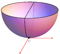
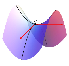
Figure 1: The energy functional is a “surface” over the “infinite dimensional manifold” of static, finite-energy field configurations. Monopoles are critical points whose (local) stability depends on the shape of the surface in the neighborhood of the critical point. For example, the critical point on Fig. 1a is stable, while that on Fig. 1b is unstable.

For a saddle point (Fig.1b) some oscillations would increase the energy; these are the stable modes. Some other ones would instead decrease the energy: there exist negative modes.

A critical point can also be degenerate, meaning that one may have zero modes, i.e. oscillations which leave the energy unchanged, cf. Fig.2.

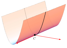
Figure 2: The energy functional can also have a flat “bottom”, whose tangent vectors are zero-modes. Other modes are positive.

The intuitive picture is that if one puts a ball into a critical point, it will roll down along energy-reducing directions, — except when it is a (local) minimum and no such directions exist.

How can we determine the type of a critical point? In finite dimensions, we would use differential calculus: a critical point is where all first partial derivatives vanish. Then the behavior of oscillations depends on the matrix of second derivatives called the Hessian,

$$\delta^{2}{\cal{E}}=\left[{\partial}_{i}{\partial}_{j}{\cal{E}}\right].$$ (1.2)

$\delta^{2}{\cal{E}}$ defines a symmetric quadratic form which is positive or negative definite if it is a [local] minimum or maximum, indefinite for a saddle point and degenerate if it has energy-preserving deformations. All this can be detected by looking at the eigenvalues of $\delta^{2}{\cal{E}}$: are they all positive, or both positive or negative, or do we have zero eigenvalues.

The number of negative modes, called the Morse index of the critical point under investigation, is denoted by $\nu$.

In Section 2 below we will apply this analysis to non-Abelian monopoles, which are critical points of the static Yang–Mills Higgs energy (2.37). Then eqn. (1.1) requires the vanishing of the first variation and yields the static Yang–Mills–Higgs field equations.

For monopoles of the ’t Hooft–Polyakov type [1, 2, 3, 4, 6] finite energy requires that on the “sphere at infinity” ${\mathds{S}}^{2}$ [meaning for large distances] the original gauge group, $G$, breaks down to the so-called “residual gauge group”, $H$. Then finite-energy YMH configurations monopoles fall into topological sectors labelled by elements of the first homotopy group of $H$,

$$\hbox{topological sectors}\sim\pi_{1}(H),$$ (1.3)

see [2, 3, 4, 14, 15, 16, 17, 18]. Each monopole solution admits, furthermore, a constant non-Abelian charge vector ${\mathds{Q}}$ introduced by Goddard, Nuyts and Olive (GNO) [19]. The GNO charge is quantized in that

$$\exp[4\pi i{\mathds{Q}}]=1,$$ (1.4)

and then the topological sector of the monopole is the homotopy class in $H$ of the loop

$$h(t)=\exp[4\pi i\,{\mathds{Q}}\,t],\qquad 0\leq t\leq 1.$$ (1.5)

Then the clue is that for certain type of variations referred to as of the “Brandt–Neri type”, the stability problem reduces to that of a pure Yang–Mills theory on the sphere at infinity with group $H$ . Then the problem boils down to studying the GNO charge, ${\mathds{Q}}$. Below we show indeed

Theorem (Goddard-Olive – Coleman) [10, 3]: For a ’t Hooft–Polyakov monopole each topological sector contains exactly one stable charge ${\stackrel{{\scriptstyle{\,\raise 0.5pt\hbox{$\scriptstyle\circ$}\,}}}{{{\mathds{Q}}}}}$.

The proof will be deduced from the formula which counts the number of negative modes,

$$\nu=\displaystyle{2\sum_{q}\left(2|q|-1\right)},$$ (1.6)

where the (half-integer) $q$ are the eigenvalues of definite sign of the $GNO$ charge ${\mathds{Q}}$ [11, 8, 9, 12]. It follows that a monopole is stable if its only eigenvalues are $0$ or $\pm 1/2$ [7, 10, 3]. All other monopoles correspond to saddle points, cf. Fig.1b.

The number of instabilities, (1.6), is conveniently counted by the so-called Bott diagram [22], see Section 5.2.

Another intuitive way of understanding monopole instability, put forward by Coleman [3], is by thinking of them as of elastic strings [3]: monopoles decay just like strings shrink, namely to the shortest one allowed by the topology, see Fig. 3.

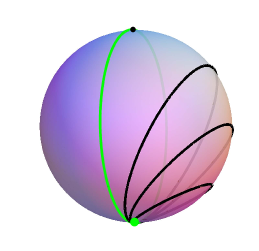
Figure 3: An elastic string wound around a sphere is in unstable equilibrium and shrinks to a point if it is perturbed.

Remarkably, this analogy can be made rigorous. Indeed, choosing a $1$-parameter family of loops $\theta\to\gamma_{\varphi}(\theta),\,0\leq\varphi\leq 2\pi$ sweeping through the two-sphere such that $\gamma_{0}=\gamma_{2\pi}$ is a point, parallel transport along $\gamma_{\varphi}$,

$$h^{A}(\varphi)={\cal P}\left(\exp\oint_{\gamma_{\varphi}}{\bm{A}}\right)\,,$$ (1.7)

associates a loop in the residual group $H$ to any YM potential ${\bm{A}}$ on ${\mathds{S}}^{2}$.

The energy of a loop in $H$ can be defined (Sec. 7) and a variational calculus, analogous to YM on ${\mathds{S}}^{2}$, can be developed. Remarkably, the map (1.7) carries monopoles i.e. critical points of the YM functional into geodesics, which are critical points of the loop-energy functional. Furthermore, the number of instabilities is also the same, namely (1.6).

The map (1.7), which has been used before [18, 2, 3, 19] for describing the topological sector of the monopole, contains much more information, however: as a matter of fact, it puts all homotopy groups of finite-energy YM configurations on ${\mathds{S}}^{2}$ and of loops in $H$ in (1-1) correspondence [23]: it is a homotopy equivalence.

1.2 Global aspects: Morse theory

A ball placed at the top of a torus will roll down to another critical point (Fig. 4b). If this is again an unstable configuration, it will continue to roll until it arrives at a stable position.

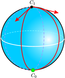
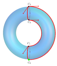
Figure 4: Global aspects of instability. A ball put to the top of a sphere (Fig.4a) or to that of a torus (Fig.4b) rolls down to some lower-lying critical point and ultimately arrives at the stable configuration. The index-$\nu=2$ critical points correspond to non-vanishing classes in the second homology group, $H_{2}$.

But what happens to an unstable monopole? By analogy, one can expect that, for sufficiently slow motion, an unstable monopole will preserve its identity and move (semi-)classically so as to decrease its energy. Although it cannot leave its topological sector since this would require infinite energy, it can go into another state in the same sector, because such configurations are separated by finite energy barriers [9].

Describing the “landscape” of static YM configurations can provide us therefore with useful information on the (possible) fate of unstable monopoles. It is tempting to think, in fact, that our energy-reducing spheres might indicate the possible decay routes of the monopole.

The stability problem can also be investigated from the global point of view. Following the Morse theory [13], for a “perfect Morse function” (of which the energy functionals of both YM on ${\mathds{S}}^{2}$ and of loops in $H$ are examples), the appearance of a critical point corresponds to a sudden change of the topology of the underlying space.

Looking at the torus (Fig.4b), one starts with the bottom with “energy” [identified with the height] ${\cal{E}}=0$. Then, for low “energies”, the section ${\cal{E}}\leq{\cal{E}}_{1}$ of the surface is contractible.

Arriving at the first critical point, $C_{1}$, however, with energy ${\cal{E}}={\cal{E}}_{1}$, the topology changes as non-contractible loops arise. Climbing higher, we reach another critical point $C_{2}$ at ${\cal{E}}={\cal{E}}_{2}$, and the topology changes once again with the arising of a different class of non-contractible loops.

Reaching the top, $C_{3}$ of the torus, ${\cal{E}}={\cal{E}}_{3}$, yet another sudden topology change takes place: we get a closed non-contractible two-surface — namely the torus itself.

In field theories, saddle-points are often associated with non-contractible loops of field configurations [24, 25, 26, 27]. The strategy is provided by the so-called “mountain-pass lemma”: consider first the highest point on each non-contractible loop; then the infimum of these tops will be a critical point, see Fig.5 .

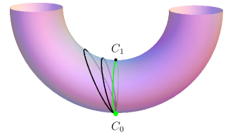
Figure 5: If one has a family of non-contractible loops all passing through the bottom, $C_{0}$, then the “mountain pass lemma” says that the infimum $C_{1}$ of the highest points on each of the loops is, under suitable conditions, an (unstable) critical point.

It is easy to see that there are no non-contractible loops in our case. There exist, however, non-contractible spheres, and in Sec. 8.1 we “hang” indeed $k$ energy reducing two-spheres at a given unstable configuration of Morse index $\nu=2k$ with their bottoms at certain other, lower-energy configurations. The tangent vectors at their top yield the required number of negative modes (cf. Fig. 4). A handy choice of the $\gamma_{\varphi}(\theta)$’s allows also to recover the loop-negative modes (explicitly constructed in Sec. 7) as images of the YM-modes.

The relation of a critical point to topology change is understood intuitively as follows [13]. Flowing down along the negative-mode directions, provides us with a small $\nu$-dimensional “cap” which, when glued to the lower-energy part of configuration space, forms a closed, $\nu$-dimensional surface cf. Fig.6.

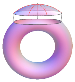
Figure 6: Flowing down from a critical point of Morse index $\nu$ along the negative-mode directions yields a $\nu$-dimensional “cap” which, when glued to the lower-energy part of the configuration space, forms a closed $\nu$-dimensional surface which generates a non-trivial homology class in $H_{\nu}$.

2 Monopoles in Unified Gauge Theories

2.1 Electric charge quantization and the Dirac Monopole

The first explanation for the quantization of the electric charge was put forward by Dirac [29], who, in 1931, posited the existence of a radial magnetic field,

$${\bm{B}}=\frac{g}{r^{2}}\,\hat{{\bm{r}}},$$ (2.8)

where the real constant $g$ is the magnetic charge,

$$g=\frac{1}{4\pi}\int_{{\mathds{S}}^{2}}{\bm{B}}\cdot d{\bm{S}}.$$ (2.9)

Note for further reference that (2.8) is in fact

$$B_{i}={g}\,{\hbox{$\textstyle\frac{1}{2}$}}\epsilon_{ijk}\omega_{jk},$$ (2.10)

where

$$\omega={\hbox{$\textstyle\frac{1}{2}$}}\omega_{ij}dx^{i}\wedge dx^{j}={\hbox{$\textstyle\frac{1}{2}$}}\,\frac{{\bm{r}}\cdot d{\bm{r}}\times d{\bm{r}}}{r^{3}}\,.$$ (2.11)

is the surface form of the two-sphere. The electromagnetic two-form $F={\hbox{$\textstyle\frac{1}{2}$}}F_{\mu\nu}dx^{\mu}\wedge dx^{\nu}$ where $F_{0i}=0,\;F_{ij}=\epsilon_{ijk}B_{k}=g\,\omega_{ij}$ satisfies therefore the vacuum Maxwell equations

$$dF=0,\qquad d\star F=0$$ (2.12)

everywhere except at the origin.

The unusual feature of this field is that $F$ does not derive from a globally well-defined vector potential. Assuming ${\bm{B}}={\rm curl\ }{\bm{A}}$ i.e. $F=dA$ for some $1$-form $A=A_{i}dx^{i}$ would indeed yield a contradiction. On the one hand, Stokes’ theorem would require

$$\int_{{\mathds{S}}^{2}}F=\int_{{\mathds{S}}^{2}}dA=\int_{\emptyset}A=0,$$

since the closed two-surface ${\mathds{S}}^{2}$ has no boundary. Direct evaluation yields, however,

$$\int_{{\mathds{S}}^{2}}F=4\pi g\neq 0,$$

a contradiction.

The clue of Dirac has been that this fact has no physical consequence provided the electric and magnetic charges, $e$ and $g$, satisfy a suitable quantization condition.

At the purely classical level, the vector potential plays no role. It does play a role at the quantum level, though, as it can be understood as follows. $dF=0$ does imply the existence of a vector potential in each contractible subset of space. Restricting ourselves to the surface of the unit two-sphere, vector potentials can be found on the “upper” and “lower” hemispheres,

$$U_{N} = \Big{\{}(\theta,\varphi)\,\Big{|}\,0\leq\theta<\pi/2+\epsilon,\,0\leq\varphi\leq 2\pi\Big{\}}$$ (2.13)

$$U_{S} = \Big{\{}(\theta,\varphi)\,\Big{|}\,\pi/2-\epsilon<\theta\leq\pi\,0\leq\varphi\leq 2\pi\Big{\}},$$ (2.14)

e.g., in polar coordinates,

$$A_{\theta}^{\pm}=0,\quad A_{\varphi}^{\pm}=g(\pm 1-\cos\theta)$$ (2.15)

in a suitable gauge. Here the $\pm$ sign refers to the N and S hemispheres, respectively.

In each coordinate patch we can describe our particle by a wave function, $\psi^{+}$ and $\psi^{-}$, respectively, each satisfying the minimally coupled Schrödinger equation

$$i\hbar{\partial}_{t}\psi^{\pm}=-\frac{{\bm{D}}^{2}}{2m}\psi^{\pm},\quad{\bm{D}}=\mbox{\boldmath$\nabla$}-ie{\bm{A}}.$$ (2.16)

In order to have a well-defined physical system, the two descriptions must be gauge-related, i.e.,

$$\psi^{+}(x)=h(x)\psi^{-}(x)$$ (2.17)

for some ${\rm U}(1)$-valued function $h(x)$ called the transition function, defined in the overlap $U^{+}\cap U^{-}$. Then

$$(e/\hbar)({\bm{A}}^{+}-{\bm{A}}^{-})=\frac{dh}{ih}\,\quad\Rightarrow\quad D^{+}\psi^{+}=h(D^{-}\psi^{-}).$$ (2.18)

if $\psi^{+}=h\psi^{-},$ so that the descriptions (2.16) are indeed equivalent. For (2.15) the condition (2.18) yields

$$h(x)=e^{i(2eg/\hbar)\varphi},$$ (2.19)

$x=(\varphi,\theta),\,0\leq\varphi\leq 2\pi,\,\pi-\epsilon<\theta<\pi+\epsilon$, whose periodicity provides us with the celebrated Dirac quantization condition

$$2eg=n\,\hbar,\quad n\in{\mathds{Z}}.$$ (2.20)

Equivalently,

$$\exp\big{[}i\oint e(A^{+}-A^{-})\big{]}=1$$ (2.21)

for any closed loop.

This same condition can also be expressed by saying that the non-integrable phase factor

$$\exp\big{[}i\oint_{\gamma}eA\big{]}$$ (2.22)

must have a gauge-independent meaning for any closed loop. Here mathematicians recognize the expression for holonomy [30, 31, 32] obtained by parallel transport; this is indeed the starting point of Wu and Yang’s “integral formulation” of gauge theory [33] .

The bundle picture [36, 37, 38, 39, 40]

The above result can be reformulated in a geometric language: (2.21) is the necessary and sufficient condition for the existence of a principal ${\rm U}(1)$ bundle ${\cal{Y}}$ with connection ${\cal{A}}$. [30, 31, 40]. Locally i.e. over a coordinate patch $U$,

$${\cal{Y}}\Big{|}_{U}=\Big{\{}(x,z)\in U\times{\rm U}(1)\Big{\}},\qquad{\cal{A}}=A+\frac{dz}{iz},$$ (2.23)

The right action of $h\ni{\rm U}(1)$ on ${\cal{Y}}$ is locally $h~{}:\zeta=(x,z)\to\zeta\cdot h=(x,zh)$.

Covering the whole base manifold (here ${\mathds{S}}^{2}$) with such patches, with $U^{+}$ and $U_{-}$ for example, condition (2.21) guarantees that

$$h(x)=\exp\big{[}ie\int_{\gamma}({\bm{A}}^{+}-{\bm{A}}^{-})\cdot dx\big{]},$$ (2.24)

where $\gamma$ is any path from a reference point $x_{0}$ to $x$ in $U^{+}\cap U^{-}$ is well-defined in that it only depends on the initial and final points but not on the path $\gamma$ itself. In fact, $h(\varphi)=\exp\big{[}i2eg\varphi\big{]}=e^{in\varphi}$ cf. (2.19) and the local gauge potentials are related as in (2.18).

Conversely, if $s:U\to{\cal{Y}}$ is a section of the bundle, then $A=s^{*}{\cal{A}}$ is a local vector potential; choosing another section yields a gauge related potential.

The wave function can also be lifted to the bundle. Setting, in a local patch,

$$\Psi(\zeta)=\psi(x)z,$$ (2.25)

provides us with an equivariant function on the bundle ${\cal{Y}}_{n}$, $\Psi(\zeta\cdot h)=h\,\Psi(\zeta)\,,\;h\in{\rm U}(1).$

The most convenient way to realize the general theory is to use the Hopf fibration [35, 38, 39, 40]: dropping the irrelevant radial variable, we consider ${\mathds{S}}^{3}$ as sitting in ${\mathds{C}}^{2}$,

$${\mathds{S}}^{3}=\Big{\{}\zeta=\left(\begin{array}[]{c}z_{1}\\ z_{2}\end{array}\right)\in{\mathds{C}}^{2}\;\Big{|}\,|z_{1}|^{2}+|z_{2}|^{2}=1\Big{\}}.$$ (2.26)

${\rm U}(1)$ acts on ${\mathds{S}}^{3}$ as $\zeta\to\zeta\cdot h=\left(\begin{array}[]{c}z_{1}h\\ z_{2}h\end{array}\right).$ The subgroup ${\mathds{Z}}_{n}=\big{\{}\exp 2\pi ik/n|0\leq k\leq n-1\big{\}}$ acts on ${\mathds{S}}^{3}$ and the quotient

$${\cal{Y}}_{n}={\mathds{S}}^{3}/{\mathds{Z}}_{n}$$ (2.27)

is therefore a principal ${\rm U}(1)$ bundle with base ${\mathds{S}}^{2}\subset{\mathds{R}}^{3}$. The projection ${\cal{Y}}_{n}\to{\mathds{S}}^{2}\subset{\mathds{R}}^{3}$ is given by

$$\pi([\zeta])_{i}=\overline{\zeta}\sigma_{i}\zeta,\qquad i=1,2,3,$$ (2.28)

where the $\sigma_{i}$ are the $2\times 2$ Pauli matrices and $\overline{\zeta}=\left({\overline{z}}_{1},{\overline{z}}_{2}\right)$. Then

$${\cal{A}}_{n}=\frac{n}{i}\,\overline{\zeta}\,d\zeta=\frac{n}{i}\big{(}{\overline{z}}_{1}dz_{1}+{\overline{z}}_{2}dz_{2}\big{)}$$ (2.29)

is a connection form on ${\cal{Y}}_{n}$ with curvature

$$d{\cal{A}}=n\omega,$$ (2.30)

i.e., $n$-times the surface form of the two-sphere. Thus ${\cal{Y}}_{n}$ has Chern class $c({\cal{Y}}_{n})=n$ [31, 32].

Parametrizing the two-sphere with Euler angles $(\theta,\varphi,\chi)$,

$$\zeta\sim\left(\begin{array}[]{c}\exp[\hbox{$\textstyle\frac{i}{2}$}(\varphi+\chi)]\cos\theta\\[6.0pt] \exp[-\hbox{$\textstyle\frac{i}{2}$}(\varphi-\chi)]\sin\theta/2\big{)}\end{array}\right),$$ (2.31)

$$s_{+}(\theta,\varphi)=\left(\begin{array}[]{c}\cos(\theta/2)\\[6.0pt] i\exp[i\varphi]\sin(\theta/2)\end{array}\right)$$ (2.32)

is a local section of our bundle such that $A^{+}=s_{+}^{*}{\cal{A}}$.

2.2 Unified gauge theories

The success of unifying weak and electric interactions into a single theory by extending the ${\rm U}(1)$ gauge group of electromagnetism into ${\rm U}(2)$ (locally ${\mathfrak{u}}(1)_{e}\oplus{\mathfrak{su}}(2)_{w}$) [41] generated an outburst of interest in attempting further unification by including strong interactions,

$$\mathfrak{h}={\mathfrak{u}}(1)_{e}\oplus{\mathfrak{su}}(2)_{w}\oplus{\mathfrak{su}}(3)_{s}$$ (2.33)

obtained from some Grand Unified gauge group $G$ as residual symmetry after spontaneous symmetry breaking by the Higgs mechanism. The most attractive ones of these Grand Unification Theories (GUT)s start with $G={\rm SU}(5)$, or ${\rm SO}(10)$ [42].

GUTs made seemingly unnecessary Dirac’s experimentally never-confirmed hypothesis, as they provided an alternative explanation of electric charge quantization. Around 1974, however, ‘t Hooft, and Polyakov [1] found that Unified Gauge Theories admit finite-energy particle-like exact solutions which for large distances behave as Dirac monopoles. Their original results show this in the context of $G={\rm SU}(2)$, later extended to more general gauge groups [43].

Below we present a brief outline of non-Abelian gauge theories and of their monopole solutions.

Let $G$ be a compact simple Lie group. A (static) Yang–Mills–Higgs theory is given by the following ingredients:

1. A (static and purely magnetic) Yang–Mills gauge field is a connection form on a $G$-bundle $P$ over space, ${\mathds{R}}^{3}$. Locally, such a connection form is given by a $1$-form $A_{i}$ with values in $\mathfrak{g}$, the Lie algebra of $G$, $A_{i}=(A_{i}^{\ a}),\ a=1,\dots,\dim(\mathfrak{g})$, represented by hermitian matrices, $\xi^{\dagger}=\xi$. The Yang–Mills field strength $F_{ij}$ is the curvature of the connection, and the magnetic field, ${\bm{B}}=(B_{i})$, is its dual,

   $$F_{ij}={\partial}_{i}A_{j}-{\partial}_{j}A_{i}+ie[A_{i},A_{j}],\qquad B_{i}^{a}={\hbox{$\textstyle\frac{1}{2}$}}\epsilon_{ijk}F_{jk}^{a},$$ (2.34)

   respectively, where $[\,\cdot\,,\,\cdot\,]$ is the commutator in the Lie algebra $\mathfrak{g}$ of $G$, and $e$ is a coupling constant.

2. A Higgs field $\Phi$ is a scalar function on $P$ which takes its values in some linear representation space $V$ of $G$, $G:V\ni\xi\to g\cdot\xi\in V$. $\Phi$ is equivariant, $\Phi(p\cdot g)=g\cdot\Phi(p)$ where $p\cdot g$ denotes the right action of $G$ on $P$. The infinitesimal [Lie algebra] action on $V$ is denoted by $\eta\cdot\xi$.

   A frequent choice is $V=\mathfrak{g}$ the Lie algebra, and then the actions are the adjoint ones,

   $${\rm Ad}_{g}(\xi)=g^{-1}\xi g\quad\hbox{and}\quad{\rm ad}_{\eta}(\xi)=-i[\eta,\xi],$$ (2.35)

   respectively. In what follows, we shall mostly consider the adjoint case, $V=\mathfrak{g}$, when $\Phi=(\Phi^{a}),\,a=1,\dots,{\rm dim}\,\mathfrak{g}$.

3. A Higgs potential $U$ is a non-negative invariant function on $V$, $U\geq 0$, $U(g\cdot\Phi)=U(\Phi)$. Then the absolute minima of $U(\Phi)$ lie in some orbit ${\cal O}\simeq G\cdot\Phi_{0}$ of $G$. This assumption that $G$ acts transitively means the orbit is identified with ${\cal O}\simeq G/H$ where $H$ is the stability subgroup of $\Phi_{0},\,H\cdot\Phi_{0}=\Phi_{0}$. In the physical context $H$ will be referred to as the residual group.

   In the simplest case $G={\rm SU}(2)$, the most frequent choice is

   $$U(\Phi)=\frac{\lambda}{4}\big{(}1-||\Phi||^{2}\big{)}^{2}$$ (2.36)

   where, for an adjoint Higgs, $||\Phi||^{2}={\,\rm Tr\,}(\Phi^{2})=\Phi^{a}\Phi^{a}$.

A (static and purely magnetic) finite-energy Yang–Mills–Higgs configuration is such that the energy,

$$\begin{array}[]{lll}{\cal{E}}&=&\displaystyle\int_{{\mathds{R}}^{3}}\Big{\{}\frac{1}{2}{{\,\rm Tr\,}}({\bm{B}}^{2})+\frac{1}{2}{{\,\rm Tr\,}}({\bm{D}}\Phi)^{2}+U(\Phi)\Big{\}}d^{3}{\bm{r}}\end{array}$$ (2.37)

is finite. Here

$$D_{i}\Phi={\partial}_{i}\Phi+ie[A_{i},\Phi]$$ (2.38)

is the covariant derivative where, for simplicity, we restricted ourselves to an adjoint Higgs field.

The energy (2.37) is invariant w.r.t. gauge transformations,

$$A_{j}\to gA_{j}g^{-1}-\frac{i}{e}g{\partial}_{j}g^{-1},\qquad\Phi\to g\cdot\Phi=g\Phi g^{-1},$$ (2.39)

which imply that ${\bm{B}}\to g{\bm{B}}g^{-1}$, ${\bm{D}}\Phi\to g\cdot{\bm{D}}\Phi$.

Monopoles arise as finite-energy solutions of the associated variational Yang–Mills–Higgs equations [1, 2, 3, 4]. Restricting ourselves, for notational simplicity, to the adjoint case, the field equations read

$${\bm{D}}\times{\bm{B}} = ie[{\bm{D}}\Phi,\Phi],$$ (2.40)

$${\bm{D}}^{2}\Phi = \frac{\delta U}{\delta\Phi}.$$ (2.41)

2.3 Finite-energy configurations

In this subsection we shall not require that the fields satisfy the field equations, but only that they be of finite energy, i.e., such that the integral in (2.37) converges. One reason for this is to emphasize that the most important spontaneous symmetry breakdown, namely that of the Higgs potential, comes from the finite energy and not from the field equations.

We shall consider the three terms in (2.37) in turn. It will be convenient to use the radial gauge ${\bm{r}}\cdot{\bm{A}}=0$.

Pure gauge term ${\,\rm Tr\,}{\bm{B}}^{2}$

For sufficiently smooth gauge fields the finite energy condition imposed by this term is, with some abuse of notation,

$${\bm{A}}({\bm{r}})\to\frac{{\bm{A}}(\theta,\varphi)}{r},\qquad{\bm{B}}({\bm{r}})\to\frac{{\bm{b}}(\theta,\varphi)}{r^{2}}=\frac{b(\theta,\varphi)}{r^{2}}\,\hat{{\bm{r}}},$$ (2.42)

where $\theta,\,\varphi$ denote the polar angles . Note that (2.42) only involves the gauge field.

Higgs potential $U(\Phi)$

The finite energy condition for this term is $r^{2}\,U(\Phi)\sim 0$ as $r\to\infty$. A necessary condition for this is that $U\to 0$. But $U\geq 0$ is assumed to be a Higgs potential i.e. one whose minima lie on some non-trivial group orbit $G/H$, where $H$ is an appropriate subgroup of $G$, called the “residual gauge group”.

At large distances the Higgs field takes therefore its values in the orbit $G/H$ and may only depend non-trivially on the polar angles: $\Phi(r,\theta,\varphi)\to\Phi(\theta,\varphi)$ as $r\to\infty$ (again with some abuse of notation). Then the asymptotic values of $\Phi$ define a map of “the two-sphere at infinity” ${\mathds{S}}^{2}_{\infty}$ parametrized with the polar angles $(\theta,\varphi)$ into the orbit $G/H$,

$$\Phi~{}:~{}{\mathds{S}}^{2}_{\infty}\to G/H.$$ (2.43)

The asymptotic values of the Higgs field define thus a homotopy class in $\pi_{2}(G/H)$. Since this class can not be changed by smooth deformations, the “manifold” of finite-energy configurations splits into topological sectors, labelled by $\pi_{2}(G/H)$ [2, 3, 4, 14, 15, 16, 17].

As

$$\pi_{2}(G/H)\simeq\pi_{1}(H)$$ (2.44)

for any [simply connected] Lie group $G$, the topological sectors can be labelled also by classes in $\pi_{1}(H)$; the first homotopy group of the residual group. Indeed, on the upper and respectively on the lower hemispheres $N$ and $S$ of ${\mathds{S}}^{2}$,

$$\Phi(\theta,\varphi)=\left\{\begin{array}[]{lll}g_{N}(\theta,\varphi)\Phi(E)&\hbox{in}&N\\[12.0pt] g_{S}(\theta,\varphi)\Phi(E)&\hbox{in}&S\end{array}\right.,$$

where (the “east pole”) $E$ is an arbitrary point in the overlap.

$$h(\varphi)=g_{N}^{-1}(\varphi)g_{S}(\varphi)$$ (2.45)

where $\varphi$ is the polar angle on the equator of ${\mathds{S}}^{2}$ is a loop in $H$ which represents the topological sector. (2.45) is contractible in $G$ [3, 2].

For any compact and connected Lie group $H$, $\pi_{1}(H)$ is Abelian so has a free part and a torsion part

$$\pi_{1}(H)={\mathds{Z}}^{p}\oplus{\mathds{T}},$$

where $p$ is the dimension of the centre of $\mathfrak{h}$ and ${\mathds{T}}$ is a finite Abelian group [17], see Section 3 below. In fact, ${\mathds{T}}$ is isomorphic to $\pi_{1}(K)$ where $K$ is the compact and semisimple subgroup of $H$ generated by $\mathfrak{k}=[\mathfrak{h},\mathfrak{h}]$.

The free part ${\mathds{Z}}^{p}$ provides us with $p$ integer “quantum” numbers $m_{1},\dots,m_{p}$. They can be calculated as surface integrals as follows. To the asymptotic physical Higgs field $\Phi$ in any representation and to each vector $\zeta$ from the centre of the Lie algebra $\mathfrak{h}$, we can associate an auxiliary adjoint “Higgs” field $\Psi$ defined by

$$\Psi_{\zeta}(\theta,\varphi)=g(\theta,\varphi)\,\zeta\,g^{-1}(\theta,\varphi),$$ (2.46)

where $g(\theta,\varphi)$ is any of those “lifts” in (2.45). Although the lifts in (2.3) are ambiguous, $gh$ works if $g$ does when $h$ belongs to $H$, $\Psi(\theta,\varphi)$ is well-defined, because $\zeta$ belongs to the centre of $\mathfrak{h}$. The projection of the charge lattice $\Gamma_{Q}$ into the centre is a $p$-dimensional lattice there, generated over the integers by $p$ vectors $\zeta_{1},\dots,\zeta_{p},$,

$$\zeta=\sum_{i=1}^{p}n_{i}\zeta_{i},\quad n_{i}\in{\mathds{Z}}$$ (2.47)

Note that the $\zeta_{a}$ are not in general charges themselves, nor are they normalized.

The above construction associates then an adjoint “Higgs” field $\Psi_{a}$ to each generator $\zeta_{a}$, and the quantum numbers $m_{a}$ are calculated according to [14, 17]

$$m_{a}=\frac{1}{4\pi|\zeta_{a}|^{3}}\int_{{\mathds{S}}^{2}}B_{a}\bigl{(}\Psi_{a},\,\bigl{[}{\partial}_{\theta}\Psi_{a},{\partial}_{\varphi}\Psi_{a}\bigr{]}\bigr{)}\,d\varphi\wedge d\theta,\qquad a=1,\dots,p,$$ (2.48)

where $\Psi_{a}$ is the auxiliary Higgs field (2.46) for $\zeta=\zeta_{a}$, $B_{a}$ is a multiple $(\alpha_{a},\alpha_{a})B/2$ of the Killing form $B$ of $G$ and $\alpha_{a}$ is a simple root determined by $\zeta_{a}$.

The mathematical content of this theorem is that the free part of $\pi_{2}({\cal O})$ has the same rank as the dimension of the second de Rham cohomology,

$$\pi_{2}({\cal O})\otimes{\mathds{R}}\simeq H_{2}({\cal O})\otimes{\mathds{R}}\simeq H^{2}_{dR}({\cal O}),$$ (2.49)

which is in turn generated by the pull-backs to the orbit ${\cal O}\simeq(G/H)$ of the canonical symplectic forms of the coadjoint orbits of the basis vectors $\zeta_{k}$ [15, 16, 17].

For a matrix group, $B$ can be replaced by the trace, for example, for $G=SU(n)$ we have

$$B(\eta,\zeta)=2n\mathop{\mathrm{Trace}}(\eta\zeta)\qquad\hbox{and}\qquad(\alpha_{k},\alpha_{k})=2$$ (2.50)

for all simple root $\alpha_{k}$. The charge (2.48) is in fact the same as

$$m_{a}=\frac{1}{2\pi|\zeta_{a}|}\int_{{\mathds{S}}^{2}}\!\Psi_{a}^{*}\Omega_{a},$$ (2.51)

where $\Omega_{a}$ is the canonical symplectic form of the coadjoint orbit ${\cal O}_{a}=Ad^{*}_{G}\,\zeta_{a}$ identified with an adjoint orbit using $(\alpha_{a},\alpha_{a})B/2$. ${\mathds{T}}$, the finite part of $\pi_{1}(H)$, has no similar expression.

The physically most relevant case is when ${\mathds{T}}=0$ and the sectors are described by a single integer quantum number $m$. This happens when the Lie algebra $\mathfrak{h}$ of $H$ has a $1$-dimensional centre generated by a single vector $\zeta$ and the semisimple subgroup $K$ is simply connected.

Another case of [mostly pedagogical] interest [3] is $H={\rm SO}(3)$, for which $p=0$ and ${\mathds{T}}={\mathds{Z}}_{2}$.

The homotopy classification is not merely convenient, but is mandatory in that the classes are separated by infinite energy barriers [9].

Note that since not only $U\to 0$ but $r^{3}U\to 0$ one has [9],

$$\Phi({\bm{r}})\to\Phi(\theta,\varphi)+\eta(r,\theta,\varphi),$$ (2.52)

where $r\eta(r,\theta,\varphi)\to 0$ as $r\to\infty$.

We stress that monopole topology only depends on the Higgs field and not on the gauge field [14, 17].

The cross-term $({\bm{D}}\Phi)^{2}$

This final term involves both $\Phi$ and ${\bm{A}}$ and it hence provides the connection between the [asymptotic] Higgs field $\Phi(\theta,\varphi)$ and the gauge field ${\bm{b}}(\theta,\varphi)$ and thus puts a topological constraint on the gauge field. This constraint may be expressed as a quantization condition as follows: the finite energy condition is easily seen to be $r^{2}({\bm{D}}\Phi)^{2}\to 0$ and thus $\Phi$ is covariantly constant on ${\mathds{S}}^{2}_{\infty}$,

$$D_{i}\Phi\equiv{\partial}_{i}\Phi+iA_{i}\cdot\Phi=0$$ (2.54)

[and hence also $D_{i}\Psi\equiv{\partial}_{i}\Psi+i[A_{i},\Phi]=0$] where, with some abuse of notations, we switched to fields and covariant derivative on the sphere at infinity involving their asymptotic values.

Then the topological quantum numbers $m_{a}$ can be expressed as [17]

$$m_{a}=\frac{1}{2\pi|\zeta|}\int_{{\mathds{S}}^{2}}\!\!dS\,{\,\rm Tr\,}(\Psi_{a}b),\qquad a=1,\dots,p.$$ (2.55)

Equation (2.55) shows that in general it is not the gauge field $B$ itself, but only its projection onto the centre that is quantized. Note that the quantization of $\displaystyle\int\!\!{\,\rm Tr\,}(\Psi_{a}b)$ is again mandatory, since the value of ${\,\rm Tr\,}(\Psi_{a}B)$ cannot be changed without violating at least one of the finite-energy conditions $r^{2}V\to 0$ or $r^{3}({\bm{D}}\Phi)^{2}\to 0$ and thus passing through an infinite energy barrier.

Notice that the value of (2.55) is actually independent of the choice of the Yang–Mills potential ${\bm{A}}$ as long as $\Phi$ is covariantly constant [17].

Note also that (2.54) i.e. ${\bm{D}}\Phi=0$ implies that one can choose a gauge such that the gauge potential, ${\bm{A}}$, takes its values in the residual Lie algebra $\mathfrak{h}$.

Then a loop representing the homotopy sector can be found by parallel transport [18, 2, 3]. Let us indeed cover ${\mathds{S}}^{2}_{\infty}$ with a $1$-parameter family of loops $\gamma_{\varphi}(\theta)$, e.g., by choosing $\gamma_{\varphi}$ to start from the north pole $N$, follow the meridian at angle $\varphi=0$ through the “east pole” $E$ down to the south pole $S$ and return then to the north pole along the meridian at angle $\varphi$, see Fig.7. The loop

$$h^{A}(\varphi)={\cal P}\left(\exp\oint_{\gamma_{\varphi}}{\bm{A}}\right)$$ (2.56)

[where ${\cal P}$ means path-ordering] then represents the topological sector.

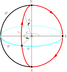
Figure 7: To any value of the angle $\varphi$ is associated a loop $\gamma_{\varphi}$ which sweeps though the entire 2-sphere as $\varphi$ varies from $0$ to $2\pi$. Since $\gamma_{0}=\gamma_{2\pi}$ is the zero loop, we get a loop of loops. Parallel transport along $\gamma_{\varphi}$, (2.56), provides us hence with a loop $h^{A}(\varphi)$ in the residual group $H$.

Other choices of the $1$-parameter family of paths $\gamma_{\varphi}$ would lead to homotopic loops $h^{A}$.

The calculation of the topological “quantum” numbers will be greatly simplified in Sec.4 devoted to solutions of the field equations.

3 Lie algebra structure and Lie group topology

Interrupting our investigations of monopoles, we digress on the first homotopy of a compact Lie group using some knowledge of its Lie algebra structure [44].

Let us indeed consider a compact simple matrix Lie algebra $\mathfrak{k}$ and choose a Cartan subalgebra $\mathfrak{t}$. A root $\alpha$ is a linear function on the complexified Cartan algebra $\mathfrak{t}^{{\mathds{C}}}$, and to each $\alpha$ is associated a vector $E_{\alpha}$ (the familiar step operator) from $\mathfrak{k}^{{\mathds{C}}}$ which satisfies, with any vector $H$ from $\mathfrak{t}^{{\mathds{C}}}$, the relation

$$\big{[}H,E_{\alpha}\big{]}=q_{\alpha}\,E_{\alpha}\,,\quad q_{\alpha}=\alpha(H).$$ (3.57)

There exists a set of primitive roots $\alpha_{i},\,i=1,\dots,r$ ($r=$ rank) such that every positive root is a linear combination of the $\alpha_{i}$ with non-negative integer coefficients i.e. $\alpha=\sum m_{i}\alpha_{i}$ for all $\alpha$.

If $\alpha$ is a root, let us define the vector $H_{\alpha}$ in $\mathfrak{t}^{{\mathds{C}}}$ by

$$\alpha(X)={\,\rm Tr\,}(H_{\alpha}X).$$ (3.58)

With suitable normalization we have

$$(E_{\alpha})^{\dagger}=E_{-\alpha}\qquad{\,\rm Tr\,}(E_{\alpha},E_{-\alpha})=1,\qquad[E_{\alpha},E_{-\alpha}]=H_{\alpha}\,.$$ (3.59)

For each root $\alpha,\,H_{\alpha}$ and the $E_{\pm\alpha}$’s form therefore [complexified] ${\mathfrak{so}}(3)^{c}$ subalgebras of $\mathfrak{k}$.

Lattice of primitive charges, $\Gamma_{P}$.

The primitive charges $P_{i}$ are defined by

$$P_{i}=\frac{2H_{i}}{{\,\rm Tr\,}(H_{i}^{2})}\quad\hbox{where}\quad H_{i}=H_{\alpha_{i}}.$$ (3.60)

The primitive charges form a natural (non-orthogonal) basis for the Cartan algebra and by adding the $E_{\alpha}$’s we get a basis for the Lie algebra $\mathfrak{k}^{{\mathds{C}}}$. The integer combinations $\sum_{i}n_{i}P_{i}$ of the primitive charges form an $r$-dimensional lattice $\Gamma_{P}$ sitting in the Cartan algebra.

Co-weight lattice, $\Gamma_{W}$.

Let us introduce next another basis for the Cartan algebra with elements $W_{i}$ dual to the primitive roots,

$$\alpha_{i}(W_{j})={\,\rm Tr\,}(H_{i}W_{j})=\delta_{ij},\qquad i,j=1,\dots,r.$$ (3.61)

Comparing (3.61) with the conventional definition [23] of primitive weights, for which there is an extra factor $(\alpha_{i},\alpha_{i})/2$ in front of the $\delta_{ij}$, one sees that the $W_{i}$’s are just re-scaled weights. They are called co-weights [10] and it is evident that they can be normalized so as to coincide with the conventional weights (by choosing $(\alpha_{i},\alpha_{i})=2$) for all groups whose roots are all of the same length, i.e. all groups except ${\rm Sp}(2r),{\rm SO}(2r+1)$, $G_{2}$ and $F_{4}$.

The integer combinations $\sum m_{i}W_{i}$ form another lattice we denote by $\Gamma_{W}$.

Since $\alpha(P_{i})$ is always an integer, the $W$-lattice actually contains the primitive-charge lattice,

$$\Gamma_{P}\subset\Gamma_{W}.$$ (3.62)

The root planes of $\mathfrak{k}$ are those vectors $X$ in the Cartan algebra for which $\alpha(X)$ is an integer, i.e., those vectors which have integer eigenvalues in the adjoint representation. The root planes intersect in the points of the $W$-lattice.

Let us stress that the weights and primitive charges only depend on the Lie algebra, and not on its global group structure. Now we define a third lattice, which does depend on the global structure.

Charge lattice, $\Gamma_{Q}$.

Denote by ${\widetilde{K}}$ the (unique) compact, simple, and simply connected Lie group generated by $\mathfrak{k}$. Any other group $K$ whose Lie algebra is $\mathfrak{k}$ is then of the form $K={\widetilde{K}}/C$, where $C$ is a subgroup of $Z=Z({\widetilde{K}})$, the centre of ${\widetilde{K}}$. $Z$ is finite and Abelian, so $C$ is always discrete. Since ${\widetilde{K}}$ is simply connected, $C$ is just $\pi_{1}(K)$, the first homotopy group of $K$.

The primitive charges satisfy the quantization condition $\widetilde{\exp}2\pi iP_{i}=1$ (exponential in ${\widetilde{K}}$) and thus also in any representation of ${\widetilde{K}}$ i.e. in any other group $K$ with the same Lie algebra. For any set $n_{i}$, $i=1,\dots,r$ of integers,

$$\exp\left[2\pi it\sum n_{i}P_{i}\right],\qquad 0\leq t\leq 1,$$ (3.63)

(exponential in $K$) is hence a contractible loop in all representations. Since any loop is homotopic to one of the form $\exp 2\pi itP,\ 0\leq t\leq 1$ where $P$ is a constant vector in $\mathfrak{k}$, we conclude that the lattice $\Gamma_{P}$ consists of the generators of contractible loops.

More generally, let us fix a group $K$ (i.e., a representation of ${\widetilde{K}}$) and define a general charge $Q$ to be an element of the Cartan algebra such that

$$\exp[2\pi iQ]=1\quad\hbox{in}\quad K,$$ (3.64)

so that $\exp[2\pi itQ],\ 0\leq t\leq 1$, is a loop, and any loop is homotopic to one of this form, as said above .

Those $Q$’s satisfying the quantization condition (3.64) [with “$\exp$” meant in $K$] form the charge lattice denoted by $\Gamma_{Q}$. It depends on the global structure, but it always contains $\Gamma_{P}$, the lattice of contractible loops. $\Gamma_{P}$ and $\Gamma_{Q}$ are actually the same for the covering group ${\widetilde{K}}$. More generally, two loops $\exp[2\pi itQ_{1}]$ and $\exp[2\pi itQ_{2}]$ are homotopic if and only if $Q_{1}-Q_{2}$ belongs to $\Gamma_{P}$, so that $\pi_{1}(K)$ is the quotient of the lattices $\Gamma_{Q}$ and $\Gamma_{P}$.

On the other hand, the charge lattice $\Gamma_{Q}$ is contained in the $W$-lattice $\Gamma_{W}$, because for any root $\alpha$ and charge $Q$,

$$1 = \big{(}\exp[2\pi iE_{\alpha}]\big{)}\big{(}\exp[2\pi iQ]\big{)}\big{(}\exp[-2\pi iE_{\alpha}]\big{)}=\exp\left[2\pi i\big{(}e^{2\pi iE_{\alpha}}Qe^{-2\pi iE_{\alpha}}\big{)}\right]$$

$$= e^{2\pi i\alpha(Q)}\exp[2\pi iE_{\alpha}]=e^{2\pi i\alpha(Q)},$$

and hence $\alpha(Q)$ is an integer.

The three lattices introduced above satisfy therefore the relation

$$\Gamma_{P}\subset\Gamma_{Q}\subset\Gamma_{W}.$$ (3.65)

In general, $\widetilde{\exp}[2\pi iW_{j}]$ is not unity in the fundamental representation of ${\widetilde{K}}$. It is however unity in the adjoint representation.

$$\widetilde{\exp}[2\pi iW_{j}]=z_{j}$$ (3.66)

belongs therefore to the centre of ${\widetilde{K}}$. Hence the two lattices $\Gamma_{P}$ and $\Gamma_{W}$ coincide for the adjoint group.

On the other hand, the correspondence $W\sim z$ can be made one-to-one by restricting the $W$’s to those ones, ${\stackrel{{\scriptstyle{\,\raise 0.5pt\hbox{$\scriptstyle\circ$}\,}}}{{W}}}$’s (say), for which the geodesics $\widetilde{\exp}[2\pi i{\stackrel{{\scriptstyle{\,\raise 0.5pt\hbox{$\scriptstyle\circ$}\,}}}{{W}}}t]\ (0\leq t\leq 1)$ are geodesics of minimal length from $1$ to $z$ i.e. for which ${\,\rm Tr\,}W^{2}$ is minimal for each $z\in Z$. (Since the weights $W$ are all of different lengths and are unique up to conjugation, the ${\stackrel{{\scriptstyle{\,\raise 0.5pt\hbox{$\scriptstyle\circ$}\,}}}{{W}}}$ for each $z\in Z$ will be unique up to conjugation). Such co-weights ${\stackrel{{\scriptstyle{\,\raise 0.5pt\hbox{$\scriptstyle\circ$}\,}}}{{W}}}$ are called minimal vectors or minimal co-weights [10], and a simple intuitive way to find them (indeed an alternative way to introduce them) is as follows.

In terms of roots $\alpha$, the $0,\pm 1$ property (which will be crucial for the stability investigation [7, 3, 10] ) may be expressed by saying that for any positive root $\alpha$,

$$\alpha({\stackrel{{\scriptstyle{\,\raise 0.5pt\hbox{$\scriptstyle\circ$}\,}}}{{W}}})=0,\pm 1.$$ (3.67)

If one considers in particular the expansion of the highest root $\theta$ in terms of the primitive roots $\alpha_{i}$, $\theta=\sum h_{i}\alpha_{i},\ h_{i}\geq 1$, and applies (3.67), one sees that $\alpha_{i}({\stackrel{{\scriptstyle{\,\raise 0.5pt\hbox{$\scriptstyle\circ$}\,}}}{{W}}})$ can be non-zero for only one primitive root, ${\stackrel{{\scriptstyle{\,\raise 0.5pt\hbox{$\scriptstyle\circ$}\,}}}{{\alpha}}}_{i}$ (say), and that the coefficient $\stackrel{{\scriptstyle{\,\raise 0.5pt\hbox{$\scriptstyle\circ$}\,}}}{{h}}_{i}$ of ${\stackrel{{\scriptstyle{\,\raise 0.5pt\hbox{$\scriptstyle\circ$}\,}}}{{\alpha}}}_{i}$ must be unity [10, 8]. This result provides us with a simple, practical method of identifying the ${\stackrel{{\scriptstyle{\,\raise 0.5pt\hbox{$\scriptstyle\circ$}\,}}}{{W}}}$’s in terms of primitive weights, namely as the duals to those primitive roots for which the coefficient in the expansion of $\theta$ is unity [10, 8].

The $W$-lattice containing the charge lattice, together with the root planes, form the Bott diagram [22] of $K$. Those vectors satisfying the “minimality” or “stability” condition (3.67) either lie in the centre or belong to the root plane which is the closest to the centre.

Magnetic monopoles belong to topological classes, described by the first homotopy group of the residual symmetry group, $H$. Now for any compact and connected Lie group $H$, $\pi_{1}(H)$ is of the form

$$\pi_{1}(H)={\mathds{Z}}^{p}\oplus{\mathds{T}},$$ (3.68)

where $p$ is the dimension of the centre $Z$ of $H$ and ${\mathds{T}}$ is a finite Abelian group [17]. In fact, ${\mathds{T}}$ is isomorphic to $\pi_{1}(K)$, where $K$ is the compact and semisimple subgroup of $H$ generated by $\mathfrak{k}=[\mathfrak{h},\mathfrak{h}]$. The free part ${\mathds{Z}}^{p}$ provides us with $p$ integer “quantum” numbers $m_{1},\dots,m_{p}$.

On the other hand, (twice) the “GNO charge” of a monopole mentioned in the previous Section is a “ charge” in the sense defined here, and belongs therefore to the charge lattice $\Gamma_{Q}$.

The projections of the charge lattice $\Gamma_{Q}$ into the centre is a $p$-dimensional lattice there, generated over the integers by $p$ vectors $\Psi_{1},\dots\Psi_{p}$. The simplest and physically most relevant case is when the homotopy group $\pi_{1}(H)$ is described by a single integer quantum number $m$. This happens when the Lie algebra $\mathfrak{h}$ of $H$ has a $1$-dimensional centre generated by a single vector $\Psi$ and the semisimple subgroup $K$ is simply connected.

Now the fundamental statement in Refs. [3, 10] says

Theorem (Goddard-Olive — Coleman): For any compact Lie group $H$, each topological sector contains an [up to conjugation] unique stable charge ${\stackrel{{\scriptstyle{\,\raise 0.5pt\hbox{$\scriptstyle\circ$}\,}}}{{Q}}}$.

Curiously, Coleman [3], stated this theorem generally, but only proved it for $H={\rm SO}(3)$, which appears spurious. Incredibly, his proof already contains the germ of the general proof [8, 9], though. The strategy is to reduce the problem to the adjoint group by factoring out the centre; this leaves us with the semisimple part alone, $\mathfrak{k}$. Now any semisimple Lie algebra can be decomposed into a sum of simple Lie algebras, $\mathfrak{k}=\mathfrak{k}_{1}+\dots+\mathfrak{k}_{s}$, and the minimal charge — which, for a simple adjoint group, is the same as a minimal co-weight — can be checked by inspection using the list of simple Lie algebras, see e.g. [44].

The examples below may help to understand the general theory outlined above.

Example 1: $H={\rm SO}(3)$

The simplest non-trivial example is when the residual Lie algebra is $\mathfrak{h}={\mathfrak{su}}(2)\simeq{\mathfrak{so}}(3)$, see Fig.8. Then the residual gauge group can be either $H={\rm SU}(2)$ which is simply connected and has therefore trivial topology. The unique minimal charge is the vacuum, ${\stackrel{{\scriptstyle{\,\raise 0.5pt\hbox{$\scriptstyle\circ$}\,}}}{{Q}}}=0$.

Non-trivial topology can, however, be obtained by changing the global structure by factoring out the centre, $Z\simeq{\mathds{Z}}_{2}$, yielding $H={\rm SO}(3)$. Then we have two topological sectors, labelled by $m=0$ and $m=1$.

In detail, the Cartan algebra of ${\mathfrak{su}}(2)$ consists of traceless diagonal matrices generated by $\sigma_{3}$. The only positive root $\alpha$ is the difference of the diagonal entries,

$$H_{\alpha}=\sigma_{3}=\left(\begin{array}[]{cc}1&0\\ 0&-1\end{array}\right),\quad E_{+}=\sigma_{+}=\left(\begin{array}[]{cc}0&1\\ 0&0\end{array}\right),\quad E_{-}=\sigma_{-}=\left(\begin{array}[]{cc}0&0\\ 1&0\end{array}\right),$$ (3.69)

generate the complexified Lie algebra ${\mathfrak{su}}(2)^{c}$. The unique minimal co-weight is

$${\stackrel{{\scriptstyle{\,\raise 0.5pt\hbox{$\scriptstyle\circ$}\,}}}{{W}}}={\hbox{$\textstyle\frac{1}{2}$}}\sigma_{3}={\hbox{$\textstyle\frac{1}{2}$}}\left(\begin{array}[]{cc}1&0\\ 0&-1\end{array}\right).$$ (3.70)

The root lattice consists of integer multiples of ${\stackrel{{\scriptstyle{\,\raise 0.5pt\hbox{$\scriptstyle\circ$}\,}}}{{W}}}$. The unique primitive charge is

$$P=2{\stackrel{{\scriptstyle{\,\raise 0.5pt\hbox{$\scriptstyle\circ$}\,}}}{{W}}}=\sigma_{3}.$$ (3.71)

The centre of ${\rm SU}(2)$ is $Z\simeq{\mathds{Z}}_{2}=\{{\mathds{1}}_{2},-{\mathds{1}}_{2}\}$ and the adjoint group, ${\rm SO}(3)\simeq{\rm SU}(2)/{\mathds{Z}}_{2}$, has two topological sectors, represented by the curves in ${\rm SU}(2)$

$$\gamma_{0}(t)=\exp[2\pi i\sigma_{3}t]\quad\hbox{and}\quad\gamma_{1}(t)=\exp[\pi i\sigma_{3}t],$$ (3.72)

$0\leq t\leq 1$, respectively. Note that while $\gamma_{0}$ is a loop in ${\rm SU}(2)$, $\gamma_{1}$ is only “half of a loop”, as it ends in $-{\mathds{1}}_{2}$. Factoring out the centre, both curves project to loops in ${\rm SO}(3)$; $\gamma_{0}$ projects into a contractible one, but $\gamma_{1}$ represents the non-trivial class $[1]$. Conversely, when lifted to ${\rm SU}(2)$, all contractible in ${\rm SO}(3)$ loops end at ${\mathds{1}}_{2}$ and the lifts of loops in the non-trivial class end at $-{\mathds{1}}_{2}$. The stable charges of the respective sectors are

$${\stackrel{{\scriptstyle{\,\raise 0.5pt\hbox{$\scriptstyle\circ$}\,}}}{{Q}}}{}^{(0)}=0\qquad\hbox{and}\qquad{\stackrel{{\scriptstyle{\,\raise 0.5pt\hbox{$\scriptstyle\circ$}\,}}}{{Q}}}{}^{(1)}={\stackrel{{\scriptstyle{\,\raise 0.5pt\hbox{$\scriptstyle\circ$}\,}}}{{W}}}={\hbox{$\textstyle\frac{1}{2}$}}\sigma_{3}.$$ (3.73)

Then any charge is

$$Q={\stackrel{{\scriptstyle{\,\raise 0.5pt\hbox{$\scriptstyle\circ$}\,}}}{{Q}}}{}^{(m)}+n{P}=\left\{\begin{array}[]{cl}n\sigma_{3}&\hbox{trivial sector}\\[8.0pt] ({\hbox{$\textstyle\frac{1}{2}$}}+n)\sigma_{3},&\hbox{nontrivial sector}\end{array}\right.$$ (3.74)

where $n$ is some integer.

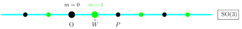
Figure 8: The Bott diagram of ${\rm SO}(3)\simeq{\rm SU}(2)/{\mathds{Z}}_{2}$, the adjoint group of ${\rm SU}(2)$. The minimal co-weight ${\stackrel{{\scriptstyle{\,\raise 0.5pt\hbox{$\scriptstyle\circ$}\,}}}{{W}}}={\stackrel{{\scriptstyle{\,\raise 0.5pt\hbox{$\scriptstyle\circ$}\,}}}{{W}}}_{1}$ is now a charge, so that $\Gamma_{W}=\Gamma_{Q}$. $\pi_{1}({\rm SO}(2))\simeq{\mathds{Z}}_{2}$, ${\stackrel{{\scriptstyle{\,\raise 0.5pt\hbox{$\scriptstyle\circ$}\,}}}{{W}}}_{0}=0$ and ${\stackrel{{\scriptstyle{\,\raise 0.5pt\hbox{$\scriptstyle\circ$}\,}}}{{W}}}$ are the minimal charges of the two topological sectors.

Example 2:  $H={\rm U}(2)$

Another simple case of considerable interest is that of when the little group $H$ of the Higgs field is $H={\rm U}(2)$. The Lie algebra is decomposed into centre plus the semisimple part, $\mathfrak{h}={\mathfrak{u}}(1)\oplus{\mathfrak{su}}(2)$, which is indeed used to describe electroweak interactions.

The Cartan algebra consists of diagonal matrices (combinations of $\sigma_{3}$ and of the unit matrix ${\mathds{1}}_{2}$). In fact, $H\in\mathfrak{t},\,E_{\pm}$ and the primitive weight ${\stackrel{{\scriptstyle{\,\raise 0.5pt\hbox{$\scriptstyle\circ$}\,}}}{{W}}}={\stackrel{{\scriptstyle{\,\raise 0.5pt\hbox{$\scriptstyle\circ$}\,}}}{{W}}}_{1}$ are as in (3.69). The only primitive vector, ${\stackrel{{\scriptstyle{\,\raise 0.5pt\hbox{$\scriptstyle\circ$}\,}}}{{W}}}_{1}$, is also a minimal one. In fact, $\exp 2\pi i{\stackrel{{\scriptstyle{\,\raise 0.5pt\hbox{$\scriptstyle\circ$}\,}}}{{W}}}_{1}=-{\mathds{1}}_{2}$. $P_{1}=2{\stackrel{{\scriptstyle{\,\raise 0.5pt\hbox{$\scriptstyle\circ$}\,}}}{{W}}}_{1}=\sigma_{3}$ generates the charge lattice of $K={\rm SU}(2)$ which is also the topological zero-sector of ${\rm U}(2)$. The topological sectors are labelled by a single integer $m$, defined by projecting onto the centre,

$$Q_{||}=m\,{\rm diag}({\hbox{$\textstyle\frac{1}{2}$}},{\hbox{$\textstyle\frac{1}{2}$}})\equiv m\,\zeta.$$ (3.75)

Note that $\zeta={\rm diag}(1/2,1/2)$ generates the centre, see Fig. 9. Note that only $2\zeta$ is a charge, $\exp[4\pi i\zeta]=1$.

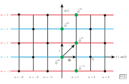
Figure 9: Bott diagram of ${\rm U}(2)$. The horizontal axis represents the Cartan algebra of ${\mathfrak{su}}(2)$, and the vertical axis is the centre generated by $\zeta={\rm diag}({\hbox{$\textstyle\frac{1}{2}$}},{\hbox{$\textstyle\frac{1}{2}$}})$. The co-weight lattice $\Gamma_{W}$ consists of the intersections all (horizontal and vertical) lines, generated by $\zeta$ and the minimal vector ${\stackrel{{\scriptstyle{\,\raise 0.5pt\hbox{$\scriptstyle\circ$}\,}}}{{W}}}\equiv W_{1}=\sigma_{3}/2$. $P=P_{1}=2{\stackrel{{\scriptstyle{\,\raise 0.5pt\hbox{$\scriptstyle\circ$}\,}}}{{W}}}=\sigma_{3}$ is the unique primitive charge. The root “planes” are vertical lines which intersect the horizontal axis at integer multiples of ${\stackrel{{\scriptstyle{\,\raise 0.5pt\hbox{$\scriptstyle\circ$}\,}}}{{W}}}$. The charges belonging to the charge lattice $\Gamma_{Q}$ and represented by dots are $Q=m\zeta+{\stackrel{{\scriptstyle{\,\raise 0.5pt\hbox{$\scriptstyle\circ$}\,}}}{{W}}}_{[m]}+nP_{1}$, where $m$ is the topological quantum number, $[m]=m$ (mod $2$), $W_{0}=0$. Those charges in the same horizontal lines are the topological sectors labelled by $m$. The pattern is periodic in $[m]$. In each topological sector, the minimal charge ${\stackrel{{\scriptstyle{\,\raise 0.5pt\hbox{$\scriptstyle\circ$}\,}}}{{Q}}}{}^{(m)}\!=m\zeta+{\stackrel{{\scriptstyle{\,\raise 0.5pt\hbox{$\scriptstyle\circ$}\,}}}{{W}}}_{[m]}$ is the one which is the closest to the centre.

The [up to conjugation] unique minimal charge of the sector $m$ is

$${\stackrel{{\scriptstyle{\,\raise 0.5pt\hbox{$\scriptstyle\circ$}\,}}}{{Q}}}{}^{(m)}=m\zeta+{\stackrel{{\scriptstyle{\,\raise 0.5pt\hbox{$\scriptstyle\circ$}\,}}}{{W}}}_{[m]}=\left\{\begin{array}[]{lll}{\rm diag\ }(k,k)&\hbox{for}&m=2k\\[8.0pt] {\rm diag\ }(k+1,k)&\hbox{for}&m=2k+1\end{array}\right.$$ (3.76)

where $[m]$ is $m$ modulo $2$ and ${\stackrel{{\scriptstyle{\,\raise 0.5pt\hbox{$\scriptstyle\circ$}\,}}}{{W}}}_{0}=0$ by convention. Any other charge of Sector $m$ is

$$Q{}^{(m)}={\stackrel{{\scriptstyle{\,\raise 0.5pt\hbox{$\scriptstyle\circ$}\,}}}{{Q}}}{}^{(m)}\!+\;{n}P_{1}={\stackrel{{\scriptstyle{\,\raise 0.5pt\hbox{$\scriptstyle\circ$}\,}}}{{Q}}}{}^{(m)}\!+\;{n}\sigma_{3}={\stackrel{{\scriptstyle{\,\raise 0.5pt\hbox{$\scriptstyle\circ$}\,}}}{{Q}}}{}^{(m)}\!+\;{\rm diag}(n,-n).$$ (3.77)

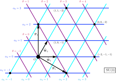
Figure 10: The Bott diagram of ${\rm SU}(3)$, generated by the minimal co-weight vectors ${\stackrel{{\scriptstyle{\,\raise 0.5pt\hbox{$\scriptstyle\circ$}\,}}}{{W}}}_{1}=\hbox{$\textstyle\frac{1}{3}$}{\rm diag}(2,-1,-1)$ and ${\stackrel{{\scriptstyle{\,\raise 0.5pt\hbox{$\scriptstyle\circ$}\,}}}{{W}}}_{2}=\hbox{$\textstyle\frac{1}{3}$}{\rm diag}(1,1,-2)$. $P_{1}={\rm diag}(1,-1,0)$ and $P_{2}={\rm diag}(0,1,-1)$ are the primitive charges and the two primitive roots are $\alpha_{1}={\,\rm Tr\,}(P_{1}\,\cdot\;)$ and $\alpha_{2}={\,\rm Tr\,}(P_{2}\,\cdot\;)$. The three families of root planes, labelled by the values of $\alpha_{1},\,\alpha_{2}$ and of the highest root $\theta$, intersect at an angle $\pi/3$. Charges and primitive charges coincide, $\Gamma_{Q}=\Gamma_{P}$.

Example 3: ${\rm SU}(3)/{\mathds{Z}}_{3}$

${\rm SU}(3)=\widetilde{K}$ is simply connected; its centre is ${\mathds{Z}}_{3}$, with elements

$$z_{0}=\hbox{\rm diag}\big{(}1,1,1\big{)},\;z_{1}=\hbox{\rm diag}\big{(}e^{4\pi i/3},e^{-2\pi i/3},e^{-2\pi i/3}\big{)},\;z_{2}=\hbox{\rm diag}\big{(}e^{2\pi i/3},e^{2\pi i/3},e^{-4\pi i/3}\big{)}.$$ (3.78)

The co-weights are now charges, so that

$$\Gamma_{W}=\Gamma_{Q}.$$ (3.79)

The adjoint group of ${\rm SU}(3)=\widetilde{K}$ is ${\rm SU}(3)/{\rm Z}$ has therefore three homotopy classes labelled by the $z_{m},\,m=1,2,3$ Each of such loop is homotopic to one of the form $\widetilde{\exp}\left[2\pi iQt\right]\,0~{}\leq~{}t~{}\leq~{}1$,

$$\widetilde{\exp}\left[2\pi iQ\right]=z_{m},$$ (3.80)

where $\widetilde{\exp}$ means the exponential in the covering group $\widetilde{K}={\rm SU}(3)$. A loop which has class $[m]\in{\mathds{Z}}_{3}$ ends at $z_{a},\,a=0,1,2$, and is homotopic to one with charge

$$Q={\stackrel{{\scriptstyle{\,\raise 0.5pt\hbox{$\scriptstyle\circ$}\,}}}{{Q}}}{}^{(m)}+n_{1}P_{1}+n_{2}P_{2}={\stackrel{{\scriptstyle{\,\raise 0.5pt\hbox{$\scriptstyle\circ$}\,}}}{{W}}}_{m}+n_{1}P_{1}+n_{2}P_{2}$$ (3.81)

The unique minimal charge of class $[m]$ is ${\stackrel{{\scriptstyle{\,\raise 0.5pt\hbox{$\scriptstyle\circ$}\,}}}{{Q}}}{}^{[m]}={\stackrel{{\scriptstyle{\,\raise 0.5pt\hbox{$\scriptstyle\circ$}\,}}}{{W}}}_{m}$.

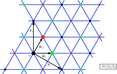
Figure 11: The Bott diagram of ${\rm SU}(3)/{\mathds{Z}}_{3}$, the adjoint group of ${\rm SU}(3)$. The root lattice is that of ${\mathfrak{su}}(3)$, with identical co-weights and primitive charges, the $W$’s and $P$’s. The only difference is that the minimal $W$’s are now charges, so that $\Gamma_{W}=\Gamma_{Q}$. $\pi_{1}({\rm SU}(3)/{\mathds{Z}}_{3})\simeq{\mathds{Z}}_{3}$ and ${\stackrel{{\scriptstyle{\,\raise 0.5pt\hbox{$\scriptstyle\circ$}\,}}}{{W}}}_{m},\ m=0,1,2,\,{\stackrel{{\scriptstyle{\,\raise 0.5pt\hbox{$\scriptstyle\circ$}\,}}}{{W}}}{}_{0}=0$ are the minimal charges of the three topological sectors. A charge in Sector $m=0,1,2$ is of the form $Q={\stackrel{{\scriptstyle{\,\raise 0.5pt\hbox{$\scriptstyle\circ$}\,}}}{{W}}}_{m}+n_{1}P_{1}+n_{2}P_{2}$.

Example 4: $H={\rm U}(3)$

A physically relevant example is when the Higgs little group is $H={\rm U}(3)$ i.e. locally ${\mathfrak{su}}(3)_{c}\oplus{\mathfrak{u}}(1)_{em}$, the symmetry of strong and electromagnetic interactions.

The diagram is now three-dimensional, the central ${\mathfrak{u}}(1)$ being the vertical axis on Fig. 12,

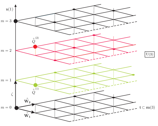
Figure 12: Bott diagram of ${\rm U}(3)$. The vertical axis represents the centre generated by $\zeta={\rm diag}(1/3,1/3,1/3)$, and the horizontal plane $\mathfrak{t}$ is the Cartan algebra of ${\rm SU}(3)$, shown in more detail on Fig. 10. The charges are $m\,\zeta+{\stackrel{{\scriptstyle{\,\raise 0.5pt\hbox{$\scriptstyle\circ$}\,}}}{{W}}}_{[m]}+n_{1}P_{1}+n_{2}P_{2}$, where $P_{1}$ and $P_{2}$ are the primitive charges of ${\rm SU}(3)$. The horizontal planes are the topological sectors. Sector $m$ is obtained from the vacuum sector by shifting by $m\,\zeta+{\stackrel{{\scriptstyle{\,\raise 0.5pt\hbox{$\scriptstyle\circ$}\,}}}{{W}}}_{[m]}$. They also coincide with the $m$ mod(3) sectors of the adjoint group, ${\rm SU}(3)/{\mathds{Z}}$. In each sector, the unique minimal charge ${\stackrel{{\scriptstyle{\,\raise 0.5pt\hbox{$\scriptstyle\circ$}\,}}}{{Q}}}{}^{(m)}$, is the one which is closest to the centre. The diagram is periodic in $m$ mod 3.

and $\mathfrak{t}$ being the horizontal plane. The primitive roots are

$$\alpha_{1}(X)=X_{1}-X_{2}\qquad\hbox{and}\qquad\alpha_{2}(X)=X_{2}-X_{3}$$ (3.82)

($X={\rm diag}(X_{1},X_{2},X_{3})$). The corresponding weight vectors,

$${\stackrel{{\scriptstyle{\,\raise 0.5pt\hbox{$\scriptstyle\circ$}\,}}}{{W}}}_{1}={\rm diag\ }(2/3,-1/3,-1/3)\qquad\hbox{and}\qquad{\stackrel{{\scriptstyle{\,\raise 0.5pt\hbox{$\scriptstyle\circ$}\,}}}{{W}}}_{2}={\rm diag\ }(1/3,1/3,-2/3)$$ (3.83)

are also minimal vectors: they exponentiate to the elements in the $Z={\mathds{Z}}_{3}$-centre of ${\rm SU}(3)$.

The highest root is $\theta=\alpha_{1}+\alpha_{2}$, and the charge lattice of $K={\rm SU}(3)$ is generated by

$$Q_{1}={\rm diag}(1,-1,0)\qquad\hbox{and}\qquad Q_{2}={\rm diag}(0,1,-1).$$ (3.84)

The topological sectors are labelled by an integer $m$. In fact, the projection of Sector $m$ onto the centre is

$$z(Q^{(m)})=m\,\zeta=m\,{\rm diag}(\hbox{$\textstyle\frac{1}{3}$},\hbox{$\textstyle\frac{1}{3}$},\hbox{$\textstyle\frac{1}{3}$}).$$ (3.85)

The unique minimal charge in sector $m$ is

$${{\stackrel{{\scriptstyle{\,\raise 0.5pt\hbox{$\scriptstyle\circ$}\,}}}{{Q}}}}{}^{(m)}=m\zeta+{\stackrel{{\scriptstyle{\,\raise 0.5pt\hbox{$\scriptstyle\circ$}\,}}}{{W}}}_{[m]}=\left\{\begin{array}[]{l}{\rm diag}(k,k,k)\\[6.0pt] {\rm diag}(k+1,k,k)\\[6.0pt] {\rm diag}(k+1,k+1,k)\end{array}\right.\quad\hbox{for}\quad m=\left\{\begin{array}[]{l}3k\\[6.0pt] 3k+1\\[6.0pt] 3k+2\end{array}\right.$$ (3.86)

where $[m]$ means $m$ modulo $3$. Any other charge is

$$Q={{\stackrel{{\scriptstyle{\,\raise 0.5pt\hbox{$\scriptstyle\circ$}\,}}}{{Q}}}}^{(m)}+Q^{\prime}={{\stackrel{{\scriptstyle{\,\raise 0.5pt\hbox{$\scriptstyle\circ$}\,}}}{{Q}}}}^{(m)}+n_{1}P_{1}+n_{2}P_{2}={{\stackrel{{\scriptstyle{\,\raise 0.5pt\hbox{$\scriptstyle\circ$}\,}}}{{Q}}}}^{(m)}+{\rm diag}(n_{1},n_{2}-n_{1},-n_{2}).$$ (3.87)

Example 5: $H=\big{(}{\rm U}(1)\times{\rm Sp}(4)\big{)}/{\mathds{Z}}_{2}$

To have a simple example where not all primitive weights are minimal, let us assume that the residual group is

$$H=\big{(}{\rm U}(1)\times{\rm Sp}(4)\big{)}/{\mathds{Z}}_{2}.$$

Then $\mathfrak{k}={\rm sp}(4)\simeq{\mathfrak{so}}(5)$, and $\widetilde{K}$ is ${\rm Spin}(5)$, the double covering of ${\rm SO}(5)$. $\mathfrak{k}$ can be represented by $4\times 4$ symplectic matrices with a $2$-dimensional Cartan algebra, say $\mathfrak{t}={\rm diag}(a,b,-a,-b)$. The charge lattice consists of those vectors in $\mathfrak{t}$ with integer entries, cf. Fig.13.

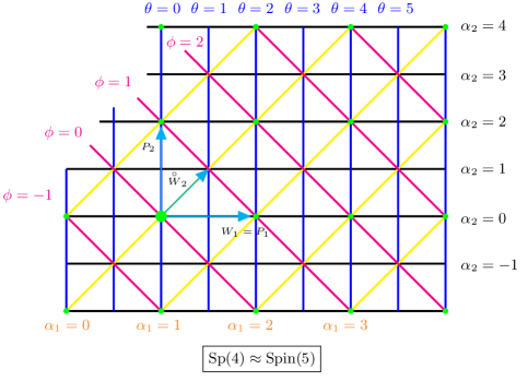
Figure 13: Bott diagram of  ${\rm Sp}(4)\simeq{\rm Spin}(5)$, the double covering of ${\rm SO}(5)$. The primitive charges are $P_{1}={\rm diag}(1,0,-1,0)$ and $P_{2}={\rm diag}(0,1,0,-1)$. The two co-weights $W$’s are $W_{1}={\rm diag}(1,0,-1,0)$ and ${\stackrel{{\scriptstyle{\,\raise 0.5pt\hbox{$\scriptstyle\circ$}\,}}}{{W}}}_{2}={\rm diag}({\hbox{$\textstyle\frac{1}{2}$}},{\hbox{$\textstyle\frac{1}{2}$}},-{\hbox{$\textstyle\frac{1}{2}$}},-{\hbox{$\textstyle\frac{1}{2}$}})$ out of which only ${\stackrel{{\scriptstyle{\,\raise 0.5pt\hbox{$\scriptstyle\circ$}\,}}}{{W}}}_{2}$ is minimal. There are $4$ families of root planes, namely $\alpha_{1}$ and $\alpha_{2}$ associated with the two co-weights, augmented with $\varphi=\alpha_{1}+\alpha_{2}$ and the highest root $\theta=2\alpha_{1}+\alpha_{2}$.

Let us choose the primitive roots $\alpha_{1}={\,\rm Tr\,}(H_{1}\,\cdot\,)$ and $\alpha_{2}={\,\rm Tr\,}(H_{2}\,\cdot\,)$, where

$$H_{1}={\hbox{$\textstyle\frac{1}{2}$}}{\rm diag}(1,-1,-1,1)\quad\hbox{and}\quad H_{2}={\hbox{$\textstyle\frac{1}{2}$}}{\rm diag}(0,1,0,-1).$$ (3.88)

These vectors dual to the primitive roots are

$$W_{1}={\hbox{$\textstyle\frac{1}{2}$}}{\rm diag}(1,0,-1,0)\quad\hbox{and}\quad{\stackrel{{\scriptstyle{\,\raise 0.5pt\hbox{$\scriptstyle\circ$}\,}}}{{W}}}_{2}={\hbox{$\textstyle\frac{1}{2}$}}{\rm diag}(1,1,-1,-1).$$ (3.89)

Then the discussion of Sec. 3 shows that only ${\stackrel{{\scriptstyle{\,\raise 0.5pt\hbox{$\scriptstyle\circ$}\,}}}{{W}}}_{2}$ is minimal: For example, only ${\stackrel{{\scriptstyle{\,\raise 0.5pt\hbox{$\scriptstyle\circ$}\,}}}{{W}}}_{2}$ exponentiates into the non-trivial element $(-{\mathds{1}})$ of Sp$(4)$:

$$\exp 2\pi W_{1}=1,\qquad\exp 2\pi{\stackrel{{\scriptstyle{\,\raise 0.5pt\hbox{$\scriptstyle\circ$}\,}}}{{W}}}_{2}=-{\mathds{1}}.$$

In other words, while $W_{1}$ is already a charge, ${\stackrel{{\scriptstyle{\,\raise 0.5pt\hbox{$\scriptstyle\circ$}\,}}}{{W}}}_{2}$ is only half-of-a-charge. Alternatively, the two remaining positive roots are $\varphi=\alpha_{1}+\alpha_{2}$ and the highest root is $\theta=2\alpha_{1}+\alpha_{2}$.

Let the integer $m$ label the topological sectors. For $m$ even, $m=2k$, the unique minimal charge belongs to the centre,

$${\stackrel{{\scriptstyle{\,\raise 0.5pt\hbox{$\scriptstyle\circ$}\,}}}{{Q}}}^{(2k)}=k\,\zeta$$ (3.90)

where $\zeta$ is a generator of the centre normalized so that $2\zeta$ is a charge.

For $m$ odd, $m=2k+1$, the unique minimal charge is rather

$${\stackrel{{\scriptstyle{\,\raise 0.5pt\hbox{$\scriptstyle\circ$}\,}}}{{Q}}}^{(2k+1)}=({k+{\hbox{$\textstyle\frac{1}{2}$}}})\,\zeta+{\hbox{$\textstyle\frac{1}{2}$}}{\stackrel{{\scriptstyle{\,\raise 0.5pt\hbox{$\scriptstyle\circ$}\,}}}{{W}}}_{2}\,.$$ (3.91)

4 Finite energy solutions: the GNO charge

Now we return to our monopole investigations.

The only condition imposed on the YMH configurations $({\bm{A}},\Phi)$ up to this point is that the energy be finite. But it is obviously of interest to consider the special case of finite energy configurations that are also solutions of the YMH field equations (2.40) – (2.41), i.e.,

$${\bm{D}}^{2}\Phi=\frac{\delta U}{\delta\Phi},\qquad{\bm{D}}\times{\bm{B}}=ie[{\bm{D}}\Phi,\Phi],$$ (4.92)

Finite energy solutions may be classified using data referring to the magnetic field alone. For this it is sufficient to consider the field equations (4.92) for large $r$. Remembering that

$${\bm{B}}({\bm{r}})\to\frac{{\bm{b}}(\theta,\varphi)}{r^{2}}=\frac{b(\theta,\varphi)}{r^{2}}\,\hat{{\bm{r}}},$$

cf. (2.42) and putting $\Phi({\bm{r}})\approx\Phi(\theta,\varphi)+\eta(r,\theta,\varphi),$ our field equations reduce to

$$\bigtriangleup\eta_{\alpha}=\left(\frac{{\partial}^{2}U}{{\partial}\Phi_{\alpha}{\partial}\Phi_{\beta}}\right)\eta_{\beta}\quad\hbox{and}\quad{\bm{D}}\times{\bm{b}}=0$$ (4.93)

in the generic case. The first equation here shows that, for solutions the generic finite-energy condition $\eta\to 0$ is sharpened to an exponential fall-off of $\eta$ .

Since $\Phi(\theta,\varphi)$ and $b(\theta,\varphi)$ are the only components of the field configuration that survive in the asymptotic region, the only possible asymptotic classification of the configurations; within each topological sector, is by $b(\theta,\varphi)$. The conditions satisfied by $b(\theta,\varphi)$ are then contained in the second equation in (4.93), which may be written as

$$D_{i}b\equiv{\partial}_{i}b+i[A_{i},b]=0.$$ (4.94)

This equation shows that $b(\theta,\varphi)$ is covariantly constant on the sphere at infinity and thus takes it values lie on an $H$-orbit. Therefore

$$b(\theta,\varphi)=\left\{\begin{array}[]{ll}h_{N}(\theta,\varphi)\,{\mathds{Q}}\,h_{N}^{-1}(\theta,\varphi)&\hbox{in}\,\,\,N\\[10.0pt] h_{S}(\theta,\varphi)\,{\mathds{Q}}\,h_{S}^{-1}(\theta,\varphi)&\hbox{in}\,\,\,S\end{array}\right.,$$

where ${\mathds{Q}}=b(E)$, the value of the magnetic field at the “east pole”, belongs to $\mathfrak{h}$. Plainly, ${\mathds{Q}}$ is unique up to global gauge rotations, and there is thus no loss of generality in choosing it in a given Cartan algebra.

In the singular gauge where $b(\theta,\varphi)={\mathds{Q}}$, the loop in (2.56) i.e. $h^{A}={\cal P}\big{(}\exp\displaystyle\oint{\bm{A}}\big{)}$ can readily be evaluated: it is simply

$$h(\varphi)=\exp[2i{\mathds{Q}}\,\varphi],\qquad 0\leq\varphi\leq 2\pi,$$ (4.95)

and the periodicity of $\varphi$ provides us with the quantization condition

$$\exp[4\pi i{\mathds{Q}}]=1$$

cf. (1.4). Using the terminology introduced in Sect. 3,

$$2{\mathds{Q}}=Q$$ (4.96)

is a charge. Conversely, any quantized ${\mathds{Q}}$ defines an asymptotic solution, namely

$${\bm{A}}={\bm{A}}^{D}{\mathds{Q}}\qquad\hbox{i.e.}\qquad A_{\theta}=0,\quad A_{\varphi}^{\pm}=(\pm 1-\cos\theta)\,{\mathds{Q}},$$ (4.97)

in the Dirac gauge, so that (4.95) is in fact the transition function. (The $\pm$ superscript refers to the northern and southern hemispheres, respectively.) Hence

$$b={\mathds{Q}}$$ (4.98)

in this gauge, and Eqns. (4.97) – (4.98) say that at infinity, the magnetic field can be gauge-transformed into a fixed direction in $\mathfrak{h}$: asymptotically, any ’t Hooft–Polyakov monopole is an imbedded Dirac monopole. In mathematical terms, the holonomy of pure YM on ${\mathds{S}}^{2}$ is one-dimensional [4] .

Solutions can thus be classified by charges of $H$. The (half)charge ${\mathds{Q}}$ was introduced by Goddard, Nuyts and Olive [19].

According to (2.55), for solutions of the field equations the expression for the “Higgs” quantum numbers $m_{a}$ reduces to

$$m_{a}=2\frac{{\,\rm Tr\,}({\mathds{Q}}\,\zeta_{a})}{{\,\rm Tr\,}(\zeta_{a}^{2})},\qquad a=1,\dots,p.$$ (4.99)

Here we would like to mention that the “topological quantum numbers” $m_{k}$’s are related to but still distinct from the magnetic charge: the latter can, in fact, only be defined by identifying the “electromagnetic” direction, which requires using a covariantly constant direction field which generates and “internal symmetry” [45]. Then, suitably defining the electric charge operator provides us with generalized [fractional] Dirac quantization conditions [2, 17, 46, 45].

We are, at last, ready to identify the minimal charge in each topological sector. Let us indeed consider a GNO charge ${\mathds{Q}}$ and denote its topological sector by $m$. let us decompose ${\mathds{Q}}$ into central and semisimple parts ${\mathds{Q}}_{||}$ and ${\mathds{Q}}_{\perp}$, respectively, ${\mathds{Q}}={\mathds{Q}}_{||}+{\mathds{Q}}_{\perp}.$ By (4.99),

$$2{\mathds{Q}}_{||}=2z({\mathds{Q}})=\sum_{k=1}^{p}m_{k}\zeta_{k}.$$

Observe that

$$z=\exp[4\pi i{\mathds{Q}}_{||}]=\exp[-4\pi i{\mathds{Q}}_{\perp}]$$ (4.100)

lies simultaneously in $Z(H)_{0}$ (the connected component of the centre of $H$) and in the semisimple subgroup $K$, and thus also in $Z(K)$, the centre of $K$. Let us decompose $\mathfrak{k}=[\mathfrak{h},\mathfrak{h}]$ into simple factors,

$$\mathfrak{k}=\mathfrak{k}_{1}\oplus\dots\oplus\mathfrak{k}_{s},$$

and denote by $\widetilde{K}_{j}$ the simple and simply connected group, whose algebra is $\mathfrak{k}_{j}$. As explained in Sec. 2, $K$ is of the form $\widetilde{K}/C$, where $C=C_{1}\times\dots\times C_{s}$ is a subgroup of the centre $Z=Z(\widetilde{K})$ of ${\widetilde{K}}=\big{[}{\widetilde{K}}_{1}\times\dots\times{\widetilde{K}}_{s}\big{]}$, $C_{j}$ being a subgroup of $Z({\widetilde{K}}_{j})$.

The situation is particularly simple when $K$ is simply connected, $K={\widetilde{K}}$, when the central part ${\mathds{Q}}_{||}$ contains all topological information. Indeed, $z$ is uniquely written in this case as

$$z=z_{1}\cdots z_{s}\qquad\hbox{where}\qquad z_{j}\in Z({\widetilde{K}}_{j}).$$ (4.101)

However, as emphasized in Sec. 3, the central elements of a simple and simply connected group are in one-to-one correspondence with the minimal ${\stackrel{{\scriptstyle{\,\raise 0.5pt\hbox{$\scriptstyle\circ$}\,}}}{{W}}}$’s and thus, for each $z$ in the centre, there exists a unique set of ${\stackrel{{\scriptstyle{\,\raise 0.5pt\hbox{$\scriptstyle\circ$}\,}}}{{W}}}_{j}$’s (where ${\stackrel{{\scriptstyle{\,\raise 0.5pt\hbox{$\scriptstyle\circ$}\,}}}{{W}}}_{j}$ is either zero or a minimal vector of $\mathfrak{k}_{j}$) such that

$$z=\big{(}\exp[-2\pi i{\stackrel{{\scriptstyle{\,\raise 0.5pt\hbox{$\scriptstyle\circ$}\,}}}{{W}}}_{1}]\big{)}\dots\big{(}\exp[-2\pi i{\stackrel{{\scriptstyle{\,\raise 0.5pt\hbox{$\scriptstyle\circ$}\,}}}{{W}}}_{s}]\big{)}=\exp\big{[}-2\pi i\sum_{k=1}^{s}{\stackrel{{\scriptstyle{\,\raise 0.5pt\hbox{$\scriptstyle\circ$}\,}}}{{W}}}_{k}\big{]}=\exp\big{[}-2\pi i{\stackrel{{\scriptstyle{\,\raise 0.5pt\hbox{$\scriptstyle\circ$}\,}}}{{W}}}{}^{(m)}\big{]}.$$ (4.102)

${\stackrel{{\scriptstyle{\,\raise 0.5pt\hbox{$\scriptstyle\circ$}\,}}}{{W}}}{}^{(m)}$ depends only on the sector (and not on ${\mathds{Q}}$ itself), because all charges of a sector have the same ${\mathds{Q}}_{||}$. Hence the entire sector can be characterized by giving

$$2{\stackrel{{\scriptstyle{\,\raise 0.5pt\hbox{$\scriptstyle\circ$}\,}}}{{{\mathds{Q}}}}}{}^{(m)}=\sum_{k}m_{k}\zeta_{k}+{\stackrel{{\scriptstyle{\,\raise 0.5pt\hbox{$\scriptstyle\circ$}\,}}}{{W}}}{}^{(m)}.$$ (4.103)

By (4.102) $2{\stackrel{{\scriptstyle{\,\raise 0.5pt\hbox{$\scriptstyle\circ$}\,}}}{{{\mathds{Q}}}}}{}^{(m)}$ is again a charge, $\exp[4\pi{\stackrel{{\scriptstyle{\,\raise 0.5pt\hbox{$\scriptstyle\circ$}\,}}}{{{\mathds{Q}}}}}{}^{(m)}]=1$, and it obviously belongs to the sector $m$. Furthermore,

$$\exp[4\pi i({\mathds{Q}}-{\stackrel{{\scriptstyle{\,\raise 0.5pt\hbox{$\scriptstyle\circ$}\,}}}{{{\mathds{Q}}}}})]=\exp[4\pi i{\mathds{Q}}]\exp[-4\pi i{\stackrel{{\scriptstyle{\,\raise 0.5pt\hbox{$\scriptstyle\circ$}\,}}}{{{\mathds{Q}}}}}]=1$$

shows that $2{\mathds{Q}}^{\prime}=2({\mathds{Q}}-{\stackrel{{\scriptstyle{\,\raise 0.5pt\hbox{$\scriptstyle\circ$}\,}}}{{{\mathds{Q}}}}})$ is in the charge lattice of $K$.

The situation is slightly more complicated if $K$ is not simply-connected, so that the semisimple part also contributes to the topology. Since $C$ is now non-trivial, the expansion (4.101) is not unique, and $z_{j}$ can be replaced rather by $z_{j}^{*}=z_{j}c_{j}$, where $c_{j}$ belongs to the subgroup $C_{j}$ of $Z({\widetilde{K}}_{j})$. But $z^{*}_{j}$ is just another element of $Z({\widetilde{K}}_{j})$, so it is uniquely $z^{*}_{j}={\stackrel{{\scriptstyle{\,\raise 0.5pt\hbox{$\scriptstyle\circ$}\,}}}{{W}}}_{j}{}^{*}$ for some minimal ${\stackrel{{\scriptstyle{\,\raise 0.5pt\hbox{$\scriptstyle\circ$}\,}}}{{W}}}_{j}{}^{*}$ of the simple factor ${\widetilde{K}}_{j}$. Equation (4.102), with all ${\stackrel{{\scriptstyle{\,\raise 0.5pt\hbox{$\scriptstyle\circ$}\,}}}{{W}}}_{j}$’s replaced by the ${\stackrel{{\scriptstyle{\,\raise 0.5pt\hbox{$\scriptstyle\circ$}\,}}}{{W}}}_{j}{}^{*}$’s, is still valid, so that (4.103) is a charge also now. However, since $\pi_{1}(K)=C=C_{1}\times\dots\times C_{s}$, those loops generated by $Q$ and $Q^{*}$ now belong to different topological sectors.

We conclude that a topological sector contains a unique charge ${\mathds{Q}}$ of the form (4.103) also in this case, and that, in full generality, any other monopole charge is uniquely of the form

$${\mathds{Q}}={\stackrel{{\scriptstyle{\,\raise 0.5pt\hbox{$\scriptstyle\circ$}\,}}}{{{\mathds{Q}}}}}+{\mathds{Q}}^{\prime}={\stackrel{{\scriptstyle{\,\raise 0.5pt\hbox{$\scriptstyle\circ$}\,}}}{{{\mathds{Q}}}}}+{\hbox{$\textstyle\frac{1}{2}$}}\sum_{i}^{r}n_{i}P_{i},$$ (4.104)

where the $n_{i}$ are integers, and the $P_{i},\,i=1,\dots r$ are the primitive charges of $K$ i.e. those which generate contractible loops in all cases. (Obviously, the $P_{i}$ are sums of primitive charges taken for the simple factors $K_{j}$). The integers $n_{i}$ could be regarded as secondary quantum numbers which supplement the Higgs charge $m$ but do not contribute to the topology.

In Sec. 5.2 we shall show that ${\stackrel{{\scriptstyle{\,\raise 0.5pt\hbox{$\scriptstyle\circ$}\,}}}{{{\mathds{Q}}}}}{}^{(m)}$ is the unique stable monopole charge in the sector $m$.

The situation is conveniently illustrated on the Bott diagram, see Section 3.

The classification of finite energy solutions according to the secondary quantum numbers or, equivalently the matrix-valued charge $Q$ is convenient and illuminating, but in contrast to the classification of finite energy configurations according to the Higgs charge $m$, it is not mandatory, in the sense that (for fixed $m$) the different charges $Q$ are separated only by finite energy barriers [9].

5 Stability analysis

5.1 Reduction from ${\mathds{R}}^{3}$ to ${\mathds{S}}^{2}$

Now we show that those monopoles for which ${\mathds{Q}}^{\prime}\neq$ are unstable. More precisely, we show that for a restricted class of variations the stability problem reduces to a corresponding Yang–Mills problem on ${\mathds{S}}^{2}$. This will allow us to prove that with respect to our variations there are

$$\nu=2\sum_{q<0}\left(2|q|-1\right)$$ (5.105)

independent negative modes [8, 11, 12] where $q$ is a negative eigenvalue of a certain operator involving the GNO charge, (5.124) below. To this end, let us first introduce the notation

$$\big{(}{\bm{a}}\times{\bm{b}}\big{)}_{i} = \varepsilon_{ijk}a_{j}b_{k},$$ (5.106)

$$\big{[}{\bm{a}}\times{\bm{b}}\big{]} = {\bm{a}}\times{\bm{b}}+{\bm{b}}\times{\bm{a}}\quad\hbox{i.e.}\quad\left(\big{[}{\bm{a}}\times{\bm{b}}\big{]}\right)_{i}=\varepsilon_{ijk}\big{[}a_{j},b_{k}\big{]}.$$

Note that ${\bm{a}}\times{\bm{a}}$ may be different from zero if $\mathfrak{h}$ is non-Abelian.

For $\mathfrak{h}$-valued variations of the gauge potentials alone of the “Brandt–Neri–Coleman type”, i.e., for

$$\delta\Phi=0,\quad\delta{\bm{A}}={\bm{a}}\in\mathfrak{h}\,,$$ (5.107)

the variations of the gauge field and covariant derivative are easily seen to be

$$\delta{\bm{B}}={\bm{D}}\times{\bm{a}},\quad\delta^{2}{\bm{B}}=-i[{\bm{a}}\times{\bm{a}}],\quad\delta({\bm{D}}\Phi)=-i[{\bm{a}},\Phi].$$ (5.108)

where, once again, we assumed for simplicity that the Higgs field belongs to the adjoint representation. All higher-order variations $\delta^{3}{\bm{B}}$ etc. are zero.

The first variation of the energy functional (2.37) is zero since $({\bm{A}},\Phi)$ is a solution of the field equations. The higher order variations are

$$\begin{array}[]{lll}\delta^{2}E&=&\displaystyle\int d^{3}{\bm{r}}\big{\{}{\,\rm Tr\,}({\bm{D}}\times{\bm{a}})^{2}-i{\,\rm Tr\,}({\bm{B}}\cdot[{\bm{a}}\times{\bm{a}}])-{\,\rm Tr\,}([{\bm{a}},\Phi])^{2}\big{\}},\\[8.0pt] \delta^{3}E&=&-3i\displaystyle\int d^{3}{\bm{r}}{\,\rm Tr\,}\big{\{}({\bm{D}}\times{\bm{a}})\cdot({\bm{a}}\times{\bm{a}})\big{\}},\\[8.0pt] \delta^{4}E&=&-3\displaystyle\int d^{3}{\bm{r}}{\,\rm Tr\,}({\bm{a}}\times{\bm{a}})^{2},\end{array}$$ (5.109)

all higher-order variations being zero. We shall assume that all variations are square-integrable and have non-zero norm,

$$0\neq({\bm{a}},{\bm{a}})=\displaystyle\int d^{3}{\bm{r}}{\,\rm Tr\,}({\bm{a}})^{2}<\infty.$$ (5.110)

There are some general points worth noting.

First, since $\delta\Phi=0$, the only terms in (5.106) involves the Higgs field is ${\,\rm Tr\,}([{\bm{a}},\Phi])^{2}$ and, in the ’t Hooft–Polyakov case $U\neq 0$, ${\bm{a}}$ must be in the little group of $\Phi(\theta,\varphi)=\lim_{r\to\infty}\Phi(r,\theta,\varphi)$, this term vanishes asymptotically. Thus, if we only consider asymptotic variations [7, 3] i.e. such that ${\bm{a}}(r,\theta,\varphi)=0$ for $r\leq R$ where $R$ is ‘sufficiently large’ so that the fields assume their asymptotic forms (2.42), the Higgs terms can then dropped in (5.109) and we shall only consider the pure Yang–Mills variations,

$$\delta^{2}E=\int d^{3}{\bm{r}}\big{\{}{\,\rm Tr\,}({\bm{D}}\times{\bm{a}})^{2}-i{\,\rm Tr\,}({\bm{B}}\cdot[{\bm{a}}\times{\bm{a}}])\big{\}}\ .$$ (5.111)

Second, the only term in (5.111) that involves radial derivatives is the $({\partial}_{r}{\bm{a}})^{2}$ term in $({\bm{D}}\times{\bm{a}})^{2}$ and this contribution may be shown to be

$$\delta^{2}E_{r}=\int d^{3}{\bm{r}}{\,\rm Tr\,}({\partial}_{r}{\bm{a}})^{2}=m^{2}({\bm{a}},{\bm{a}}),\qquad m^{2}=\hbox{$\textstyle\frac{1}{4}$}+\delta^{2}$$ (5.112)

where $\delta^{2}>0$ whose infimum of is $0$ [3, 9]. Thus, although $\delta^{2}E_{r}$ is not negligible, it can be regarded as a mass term. Therefore, for each value of $r$, the variations (5.111) are essentially variations on the $2$-sphere at infinity, ${\mathds{S}}^{2}$.

Finally, it should be noted that the variations ${\bm{a}}={\bm{D}}\chi$ where $\chi$ is any scalar, are simply gauge transformations of the background field ${\bm{A}}$ and leave the energy unchanged. In particular, it is easy to verify that, because ${\bm{A}}$ satisfies the field equations, the second variation $\delta^{2}E$ is zero for the infinitesimal variations $\delta{\bm{A}}={\bm{D}}\chi$. It is therefore convenient to define the ‘physical’ variations ${\bm{a}}$ as those which are orthogonal to the ${\bm{D}}\chi$. Using partial integration,

$$0=\displaystyle\int d^{3}{\bm{r}}{\,\rm Tr\,}({\bm{a}}\cdot{\bm{D}}\chi)=-\displaystyle\int d^{3}{\bm{r}}{\,\rm Tr\,}({\bm{D}}\cdot{\bm{a}}\,\chi)\quad\Rightarrow\,\quad{\bm{D}}\cdot{\bm{a}}=0,$$ (5.113)

since $\chi$ is arbitrary. The physical variations may also be characterized as those which are divergence-free. As a consequence of the gauge condition $A_{r}=0$ our variations satisfy also $a_{r}=0$.

It will be convenient to split (5.111) into two terms,

$$\delta^{2}E=\underbrace{\displaystyle\int d^{3}{\bm{r}}{\,\rm Tr\,}\left\{({\bm{D}}\times{\bm{a}})^{2}+({\bm{D}}\cdot{\bm{a}})^{2}\right\}}_{\delta^{2}E_{1}\geq 0}+\underbrace{\displaystyle\int d^{3}{\bm{r}}{\,\rm Tr\,}\left\{-i{\bm{B}}[{\bm{a}}\times{\bm{a}}]-({\bm{D}}\cdot{\bm{a}})^{2}\right\}}_{\delta^{2}E_{2}},$$ (5.114)

bearing in mind that ${\bm{D}}\cdot{\bm{a}}$ is unphysical and may be gauged to zero.

Let us first consider $\delta^{2}E_{1}$. From the identity

$$\big{(}{\bm{D}}\times({\bm{D}}\times{\bm{a}})\big{)}_{j}=-{\bm{D}}^{2}a_{j}+D_{j}({\bm{D}}\cdot{\bm{a}})-i\big{(}[{\bm{B}}\times{\bm{a}}]\big{)}_{j}$$ (5.115)

we have

$$\delta^{2}E_{1}=\int d^{3}{\bm{r}}{\,\rm Tr\,}\left\{(-{\bm{D}}^{2}{\bm{a}}-i[{\bm{B}}\times{\bm{a}}])\cdot{\bm{a}}\right\},$$ (5.116)

and putting ${\bm{b}}=\lim_{r\to\infty}r^{2}{{\bm{B}}}$ yields

$$\delta^{2}E_{1}=\delta^{2}E_{r}+\underbrace{\int d^{3}{\bm{r}}\,r^{-2}{\,\rm Tr\,}\left\{\big{(}{\bm{L}}^{2}{\bm{a}}-i[{\bm{b}}\times{\bm{a}}]\big{)}\cdot{\bm{a}}\right\}}_{\delta^{2}E_{S}}\,,$$ (5.117)

where ${\bm{L}}=-i{\bm{r}}\times{\bm{D}}$ is the orbital angular momentum. ${\bm{L}}$ is neither conserved nor does it satisfy the ${\mathfrak{so}}(3)$ algebra. For spherically symmetric (and hence for asymptotic) fields, the components of the angular momentum for a spinless particle ,

$$M_{i}=L_{i}-\frac{x_{i}}{r}\,b,$$ (5.118)

satisfy the ${\mathfrak{so}}(3)$ algebra $\big{[}M_{i},M_{j}\big{]}=\varepsilon_{ijk}M_{k}.$ For arbitrary variations ${\bm{a}}$ the spectrum of $\delta^{2}E_{1}$ is conveniently obtained by using instead the spin-$1$ angular momentum operator

$${\bm{J}}={\bm{M}}+{\bm{S}}=-i{\bm{r}}\times{\bm{D}}-{\bm{b}}+{\bm{S}}$$ (5.119)

where ${\bm{S}}$ is the $3\times 3$ spin matrix $\big{(}{\bm{S}}_{i}\big{)}_{jk}=i\varepsilon_{ijk}$. ${\bm{S}}$ satisfies the relations

$$[S_{i},S_{j}]=i\varepsilon_{ijk}S_{k},\quad({\bm{b}}\cdot{\bm{S}}){\bm{a}}=(b_{i}S_{i}){\bm{a}}=i[{\bm{b}}\times{\bm{a}}],\quad{\bm{S}}^{2}=S_{i}S_{i}=-2.$$ (5.120)

Using the gauge conditions ${\bm{D}}\cdot{\bm{a}}$ and ${\bm{r}}\cdot{\bm{a}}=0$, we see that

$$({\bm{r}}\times{\bm{D}})\times{\bm{a}}={\bm{r}}({\bm{D}}\cdot{\bm{a}})-r_{i}{\bm{D}}a_{i}=-r_{i}{\bm{D}}a_{i}={\bm{a}}-{\bm{D}}({\bm{r}}\cdot{\bm{a}})={\bm{a}},$$ (5.121)

i.e., ${\bm{L}}\cdot{\bm{S}}=1$. Since ${\bm{r}}$ and ${\bm{L}}$ and thus ${\bm{b}}$ and ${\bm{L}}$ are orthogonal, this implies,

$${\bm{J}}^{2}{\bm{a}}={\bm{L}}^{2}{\bm{a}}+[{\bm{b}}\times[{\bm{b}}\times{\bm{a}}]]-2i[{\bm{b}}\times{\bm{a}}].$$ (5.122)

This leads finally to rewriting $\delta^{2}E_{S}$ as

$$\delta^{2}E_{S}=\int d^{3}{\bm{r}}r^{-2}{\,\rm Tr\,}\Big{\{}\big{(}{\bm{J}}^{2}{\bm{a}}-[{\bm{b}}\times[{\bm{b}}\times{\bm{a}}]]+i[{\bm{b}}\times{\bm{a}}]\big{)}\cdot{\bm{a}}\Big{\}}\,.$$ (5.123)

It is convenient to decompose the variation ${\bm{a}}$ into eigenmodes of the operator $[{\bm{b}}\times\,\cdot\,]$ which combines vector product and Lie algebra commutator, i.e., to write

$$-i[{\bm{b}}\times{\bm{a}}]=q\,{\bm{a}}\,,$$ (5.124)

where the $q$’s are the eigenvalues. The $q$’s come in fact in pairs of opposite sign and multiplicity $2$ i.e. in quadruplets $(q,q,-q,-q)$, see the next Section.

On each $q$-sector $\delta^{2}E_{1}$ will be

$$\delta^{2}E_{1}=m^{2}({\bm{a}},{\bm{a}})+\int d^{3}{\bm{r}}{\,\rm Tr\,}\Big{\{}\big{(}\{{\bm{J}}^{2}-q(q+1)\}{\bm{a}}\big{)}\cdot{\bm{a}}\Big{\}}.$$ (5.125)

But ${\bm{J}}$ is the Casimir of the angular momentum algebra generated by ${\bm{J}}$, so ${\bm{J}}^{2}=j(j+1)$, where $j$ is integer or half-integer, according as $q$ is integer or half-integer. Now since $\delta^{2}E_{1}$ is manifestly positive by (5.114), we must have

$$m^{2}+\big{\{}{\bm{J}}^{2}-q(q+1)\big{\}}=\big{\{}\hbox{$\textstyle\frac{1}{4}$}+\delta^{2}\big{\}}+\big{\{}j(j+1)-q(q+1)\big{)}\geq 0$$ (5.126)

and since $\delta^{2}$ is arbitrarily small, we see that $j\geq|q|-1$.

Equation (5.126) implies that the possible values of $j$ are $|q|-1,|q|,|q|+1,\dots$. In particular, the value of $j=|q|-1$ can occur only for $q\leq-1$, and as it corresponds to the case when $\delta^{2}E_{1}$ is purely radial since $j(j+1)=(-q-1)(-q)=q(q+1)$, it implies that ${\bm{D}}\cdot{\bm{a}}=0$, so that the states corresponding to it are physical. Thus we can write

$$\delta^{2}E_{1}=m^{2}({\bm{a}},{\bm{a}})\quad\hbox{for}\quad j=|q|-1,\quad q\leq-1$$ (5.127)

and

$$\delta^{2}E_{1}=\big{\{}m^{2}+(j-q)(j+q+1)\big{\}}({\bm{a}},{\bm{a}})\quad\hbox{for}\quad j\geq|q|\ .$$ (5.128)

Let us now consider the second term, $\delta^{2}E_{2}$, in the decomposition (5.114) of the Hessian. Since ${\bm{D}}\cdot{\bm{a}}$ is zero on the physical states,

$$\delta^{2}E_{2} = (-i)\int d^{3}{\bm{r}}{\,\rm Tr\,}\big{(}{\bm{B}}\cdot\big{[}{\bm{a}}\times{\bm{a}}\big{]}\big{)}=\int d^{3}{\bm{r}}{\,\rm Tr\,}\left\{-i\big{[}{\bm{B}}\times{\bm{a}}\big{]}\cdot{\bm{a}}\right\}$$ (5.129)

$$= \int d^{3}{\bm{r}}\,r^{-2}{\,\rm Tr\,}\left\{-i\big{[}{\bm{b}}\times{\bm{a}}\big{]}\cdot{\bm{a}}\right\}=q\int d^{3}{\bm{r}}\,r^{-2}{\,\rm Tr\,}\big{(}{\bm{a}}^{2}\big{)}=q\big{(}{\bm{a}},{\bm{a}}\big{)}.$$

From the positivity of $\delta^{2}E_{1}$ we then see that the Hessian $\delta^{2}E$ will be positive unless $q$ is negative. Furthermore, when $q$ is negative, (5.128) becomes

$$\delta^{2}E_{1}=\big{\{}m^{2}+(j+|q|)(j-|q|+1\big{\}}\big{(}{\bm{a}},{\bm{a}}\big{)},$$ (5.130)

and hence

$$\delta^{2}E_{1}\geq 2|q|({\bm{a}},{\bm{a}})\quad\hbox{for}\quad j\geq|q|.$$ (5.131)

For $j\geq|q|$, the restriction of $\delta^{2}E_{1}$ to the physical states will therefore dominate $\delta^{2}E_{2}$ and the Hessian will again be positive. It follows that the only possibility for getting negative modes is to have

$$q\leq-1\qquad\text{and}\qquad j=|q|-1,$$ (5.132)

in which case

$$\delta^{2}E=\big{(}m^{2}-|q|\big{)}\big{(}{\bm{a}},{\bm{a}}\big{)}<0.$$ (5.133)

In conclusion, observing that the eigenvalues $q$ come in pairs of opposite sign, we have finally the result that the monopole is unstable if and only if there is an eigenvalue such that $|q|\geq 1$. The opposite condition,

$$|q|\leq{\hbox{$\textstyle\frac{1}{2}$}}\,,$$ (5.134)

is, of course, just the Brandt–Neri stability condition [7, 3, 10]. From the discussion of Sec. 2.3. we know however that $|q|\leq{\hbox{$\textstyle\frac{1}{2}$}}$ if and only if

$${\mathds{Q}}={\stackrel{{\scriptstyle{\,\raise 0.5pt\hbox{$\scriptstyle\circ$}\,}}}{{{\mathds{Q}}}}}$$ (5.135)

i.e., ${\mathds{Q}}$ is the [up to conjugation] unique stable charge of the given topological sector, cf. (4.102).

Note that since, in the case $j=|q|-1$, the first term on the right-hand side of (5.114) vanishes the variation actually satisfies the first-order equations

$${\bm{D}}\times{\bm{a}}=0,\qquad{\bm{D}}\cdot{\bm{a}}=0,$$ (5.136)

where $r{\bm{D}}=\widetilde{{\bm{D}}}\to{\bm{D}}$ is [with some abuse of notation] the covariant derivative acting on the asymptotic fields defined over the sphere at infinity. (5.136) says in particular that our ${\bm{a}}$’s are true physical modes, which form furthermore a

$$2j+1=2|q|-1$$ (5.137)

dimensional multiplet of the ${\bm{J}}$ algebra. We shall see in the next Section that for each $|q|$ there is one and only one such multiplet. Taking into account the fact that the eigenvalues come in pairs, this proves the index formula (5.105) .

The simplest way of counting the number of instabilities for $j\geq|q|$ is to use the Bott diagram (see the examples of Sec. 8.3): the Morse index $\nu$ in (5.105) is twice the number of times the straight line drawn from $2{\mathds{Q}}$ to the origin intersects the root planes [22].

In the sequel, we will work on the sphere at infinity and, with some abuse, we use the word “monopole” for a solution of the pure Yang–Mills equations with gauge group $H$ on ${\mathds{S}}^{2}$.

Let us note for further reference that the first-order equations in (5.136) are plainly consistent with the vanishing of the first term in the decomposition (5.114), and then the negative value of the Hessian $\delta^{2}E$ comes from the second term, $\delta^{2}E_{2}$. We also stress that all our investigations assume that ${\bm{a}}$ is a variation with non-zero norm, cf. (5.110). The meaning of this subtle condition will be clarified in the next Subsection.

5.2 Negative modes

Our strategy for finding our negative modes is therefore:

1. First, we find the eigenmodes of the combined operator $-i[{\bm{b}}\times\,\cdot\,]$ in (5.124) with eigenvalues $q\leq-1$;

2. Next, we solve the two coupled first-order equations (5.136) which set the first term in (5.114) to zero.

This amounts to finding the negative eigenmodes of the linear second variation operator,

$${\cal K}{\bm{a}}={\bm{J}}^{2}{\bm{a}}-[{\bm{b}}\times[{\bm{b}}\times{\bm{a}}]]+i[{\bm{b}}\times{\bm{a}}].$$ (5.139)

From the technical point of view, our goal can conveniently be achieved by complexifying the Lie algebra $\mathfrak{h}$. But then we have to make sure that our eigenmodes are indeed real and have non-vanishing norm, cf. (5.110) .

To find our negative modes, it is convenient to use the stereographic coordinate $z$ on ${\mathds{S}}^{2}$,

$$z=x+iy=e^{i\varphi}\tan\theta/2.$$ (5.141)

In stereographic coordinates the background gauge-potential and field strength become

$$A_{z}=-i{\mathds{Q}}\displaystyle\frac{{\overline{z}}}{\varrho},\quad A_{{\overline{z}}}=i{\mathds{Q}}\displaystyle\frac{z}{\varrho},\quad b=2i\displaystyle\frac{{\mathds{Q}}}{\varrho^{2}},\quad\varrho=1+z{\overline{z}},$$ (5.142)

where we treated $z$ and its conjugate ${\overline{z}}$ as independent variables. Set ${\partial}={\partial}_{z},\ \bar{\partial}={\partial}_{{\overline{z}}}$, and let us define

$$\begin{array}[]{lllllll}D_{z}&=&{\partial}-iA_{z}={\partial}-{\mathds{Q}}\displaystyle\frac{{\overline{z}}}{\varrho},&&a_{z}&=&{\hbox{$\textstyle\frac{1}{2}$}}(a_{x}-ia_{y})\\[12.0pt] D_{{\overline{z}}}&=&\bar{\partial}-iA_{{\overline{z}}}=\bar{\partial}+{\mathds{Q}}\displaystyle\frac{z}{\varrho},&&a_{{\overline{z}}}&=&{\hbox{$\textstyle\frac{1}{2}$}}(a_{x}+ia_{y})\end{array}\,.$$ (5.143)

In complex coordinates the eigenspace-equations (5.124) decouple and indeed become

$$\left(\begin{array}[]{cc}{\mathds{Q}}&0\\ 0&-{\mathds{Q}}\end{array}\right)\left(\begin{array}[]{c}a_{{\overline{z}}}\\ a_{z}\end{array}\right)=q\left(\begin{array}[]{c}a_{{\overline{z}}}\\ a_{z}\end{array}\right).$$ (5.144)

The general solution of (5.144) is

$$\left(\begin{array}[]{c}a_{{\overline{z}}}\\ a_{z}\end{array}\right)=f\left(\begin{array}[]{c}E_{\alpha}\\ 0\end{array}\right)+g\left(\begin{array}[]{c}0\\ E_{-\alpha}\end{array}\right)\qquad\text{with eigenvalue}\;\;\alpha({\mathds{Q}})$$ (5.145)

where $f$ and $g$ are arbitrary functions of $z$ and ${\overline{z}}$. Similarly,

$$\left(\begin{array}[]{c}a_{{\overline{z}}}\\ a_{z}\end{array}\right)=h\left(\begin{array}[]{c}E_{-\alpha}\\ 0\end{array}\right)+k\left(\begin{array}[]{c}0\\ E_{\alpha}\end{array}\right)\qquad\text{with eigenvalue}\;\;-\alpha({\mathds{Q}})$$ (5.146)

where $h$ and $k$ are again arbitrary. These equations show that the eigenvalues come indeed in pairs as stated earlier. Then we should select those pairs for which the eigenvalue, $q$, is negative.

As discussed in Sec. 5.1, for each fixed eigenvalue $q\leq-1$, the negative modes are solutions to the two coupled first-order equations in (5.136) which are, furthermore, equivalent to

$$D_{z}h=(\varrho\,{\partial}+|q|{\overline{z}})h=0\quad\hbox{and}\quad D_{{\overline{z}}}k=(\varrho\,\bar{\partial}+|q|z)k=0$$ (5.147)

($q=-|q|$ because $q$ is negative). One sees that $h$ and $k$ must be of the form

$$h(z,{\overline{z}})=\varrho^{-|q|}\Phi({\overline{z}}),\qquad k(z,{\overline{z}})=\varrho^{-|q|}\Psi(z),$$ (5.148)

where $\Phi({\overline{z}})$ and $\Psi(z)$ are arbitrary antiholomorphic (respectively holomorphic) functions. They can be therefore expanded into power series,

$$\Phi({\overline{z}})=\sum c_{n}{{\overline{z}}}^{n},\quad\hbox{and}\quad\Psi(z)=\sum d_{m}z^{m}.$$

But they are also square integrable functions. Now, since in stereographic coordinates, the inner product for two vector fields is

$$({\bm{a}},{\bm{b}})=\int dzd{\overline{z}}\sqrt{g}g^{\alpha\beta}a_{\alpha}\bar{b}_{\beta}=\int dzd{\overline{z}}\,a_{\alpha}\bar{b}_{\alpha}=\int dzd{\overline{z}}\,(a_{z}b_{{\overline{z}}}+a_{{\overline{z}}}b_{z}),$$ (5.149)

because $\sqrt{g}g^{\alpha\beta}$ is unity, one sees that $\Phi({\overline{z}})$ will be square integrable if, and only if, $c_{n},\ d_{m}=0$ except for $n,m=0,1,\dots,2|q|-2$. Thus, assuming

$$\alpha({\mathds{Q}})>0,$$ (5.150)

for definiteness, it is the combination (5.146) that has to be chosen; the negative modes of the operator ${\cal K}$ are linear combinations of the $2(2|q|-1)$ variations

$$\left(\begin{array}[]{c}a_{{\overline{z}}}\\ 0\end{array}\right)=\frac{{{\overline{z}}}^{n}}{(1+z{\overline{z}})^{|q|}}\left(\begin{array}[]{c}E_{-\alpha}\\ 0\end{array}\right),\qquad\left(\begin{array}[]{c}0\\ a_{z}\end{array}\right)=\frac{{z}^{m}}{(1+z{\overline{z}})^{|q|}}\left(\begin{array}[]{c}0\\ E_{\alpha}\end{array}\right),$$ (5.159)

$n,m=0,1,\dots,2|q|-2$ .

But are these the modes we were looking for? To answer this question, we must remember our conditions listed at the beginning of Sec. 5.2: firstly, they should be real, and secondly, they should have nonzero norm.

The modes in (5.159) satisfy neither of these conditions: they belong to the complexified Lie algebra $\mathfrak{h}^{c}$ and not to its real part. And they also have zero norm, since they lie in the $E_{\alpha}$ direction, and ${\,\rm Tr\,}(E_{\alpha}^{2})=0$ for any root $\alpha$. Happily enough, both defects can be cured by mixing our modes: it is easy to check that

$$\left(\begin{array}[]{c}a^{+}\\[6.0pt] a^{-}\end{array}\right)=\left(\begin{array}[]{c}a_{z}+a_{{\overline{z}}}\\[6.0pt] -i(a_{z}-a_{{\overline{z}}})\end{array}\right)=\frac{1}{(1+z{\overline{z}})^{|q|}}\left(\begin{array}[]{c}z^{n}E_{\alpha}+{\overline{z}}^{n}E_{-\alpha}\\[6.0pt] -i(z^{n}E_{\alpha}-{\overline{z}}^{n}E_{-\alpha})\end{array}\right)$$ (5.160)

are both real and have nonzero norm, as it follows from the Lie algebra relations (3.59).

In conclusion, these are the negative modes we were looking for.

We only mention that the remaining eigenspace of the Hessian can also be determined [9].

5.3 Supersymmetric interpretation of the negative modes

We conclude this section by mentioning that the Morse [instability] index $2|q|-1$ is also the Witten index for supersymmetry and the Atiyah-Singer index for the Dirac operator. Indeed, let us consider the part of $\delta^{2}E_{S}$ of the Hessian, which played a central role in Sec. 5.1. From Eq. (5.117) one may write, after some transformations,

$$\delta^{2}E_{S}=\displaystyle\int r^{2}dr\,K,\quad K=\int dzd{\overline{z}}\,\varrho^{2}{\,\rm Tr\,}(\Psi,({\cal H}\Psi)^{\dagger}),\quad{\cal H}=-{\hbox{$\textstyle\frac{1}{2}$}}\Big{\{}{\cal{Q}}^{+},{\cal{Q}}^{-}\Big{\}},$$ (5.161)

where

$${\cal{Q}}^{+}=\left(\begin{array}[]{cc}0&D_{\overline{z}}\\ 0&0\end{array}\right),\quad{\cal{Q}}^{-}=\left(\begin{array}[]{cc}0&0\\ D_{z}&0\end{array}\right),\quad\Psi=\left(\begin{array}[]{c}a_{\overline{z}}\\ a_{z}\end{array}\right).$$ (5.162)

The multiplicity $\nu$ of the ground state, the latter being a square integrable solution of

$${\cal{Q}}^{+}\Psi=\left(\begin{array}[]{c}D_{\overline{z}}a_{z}\\ 0\end{array}\right)=0,\qquad{\cal{Q}}^{-}\Psi=\left(\begin{array}[]{c}0\\ D_{z}a_{\overline{z}}\end{array}\right)=0,$$ (5.163)

is called the Witten index. But these are just the negative-mode equations (5.147). The result $\nu=2|q|-1$ is consistent with that found in Ref. [49] for supersymmetric QM on the sphere. Observe that the supersymmetric Hamiltonian ${\cal H}$ can also be written as

$${\cal H}=-{\hbox{$\textstyle\frac{1}{2}$}}{{D\mkern-2.0mu\hbox to0.0pt{\hss{\raise 0.5pt\hbox{\big{/}}}}\mkern 2.0mu}}^{2}\quad\hbox{where}\quad{D\mkern-2.0mu\hbox to0.0pt{\hss{\raise 0.5pt\hbox{\big{/}}}}\mkern 2.0mu}=D_{\overline{z}}\sigma_{+}+D_{z}\sigma_{-}=\left(\begin{array}[]{cc}0&D_{\overline{z}}\\ D_{z}&0\end{array}\right)$$ (5.164)

is a Dirac-type operator, and the negative modes are exactly those satisfying

$${D\mkern-2.0mu\hbox to0.0pt{\hss{\raise 0.5pt\hbox{\big{/}}}}\mkern 2.0mu}\Psi=0.$$ (5.165)

The number of solutions of (5.165) is the Atiyah-Singer (AS) index. The result $2|q|-1$ is obtained by the same calculation as the one in Atiyah and Bott [20], which is valid for an arbitrary Riemann surface. See also [21].

It is worth mentioning that supersymmetry is a useful tool to describe both the fluctuations around a self-dual (BPS) monopole [50], as well as the scattering of BPS monopoles [51].

6 The geometric picture: YM on ${\mathds{S}}^{2}$

The aim of this section is to present an alternative approach [8] devised for more geometrically-minded readers and close to the spirit of Atiyah and Bott’s generalization to Riemann surfaces [20]. To make this Section self-contained, we present full (and somewhat redundant) proofs.

Consider indeed pure YM theory of the two-sphere at infinity with gauge group $H$. Geometrically, the YM potential is a connection $1$-form still denoted by $A$ on a principal $H$-bundle $P$ over ${\mathds{S}}^{2}\equiv{\mathds{S}}^{2}_{\infty}$. The YM action is

$${\cal A}=\int_{{\mathds{S}}^{2}}{\,\rm Tr\,}(F\wedge\star F),$$ (6.166)

where $F=DA$ is the curvature $2$-form, and $\star$ is the Hodge duality operator on ${\mathds{S}}^{2}$. The associated field equation reads

$$D^{\star}F=0.$$ (6.167)

Now we can state again the geometric form of the GNO theorem,

Theorem (GNO [19]): In a suitable gauge the general solution of the Yang-Mills equations (6.167) is

$$F=i{\mathds{Q}}\,\omega\,,$$ (6.168)

where $\omega$ is the canonical surface form of the two-sphere and ${\mathds{Q}}$ is a constant vector in the Lie algebra $\mathfrak{h}$, quantized as in (1.4),

$$\exp[4\pi i{\mathds{Q}}]=1.$$ (6.169)

Proof: Our clue is that the YM equation (6.167) can indeed be written as

$$D{\star}F=0$$ (6.170)

since the adjoint operator $D^{\star}$ is $-\star D\star$ on the two-sphere. The field strength $F={\hbox{$\textstyle\frac{1}{2}$}}F_{\mu\nu}dx^{\mu}\wedge dx^{\nu}$ is a two-form on ${\mathds{S}}^{2}$ and therefore

$$F=b(\theta,\varphi)\,\omega$$ (6.171)

for some $\mathfrak{h}$-valued function [zero-form] $b=b(\theta,\varphi)$ on the sphere. Then the Hodge dual of $F$ is precisely $b$,

$$\star F=b(\theta,\varphi),$$ (6.172)

because the dual of the canonical surface form of the sphere is $\star\omega=1$, as it can be verified writing $\omega$ either in polar or complex coordinates,

$$\omega={\hbox{$\textstyle\frac{1}{2}$}}\sin\theta\,d\theta\wedge d\varphi=\frac{1}{i}\frac{dz\wedge d{{\overline{z}}}}{(1+z{\overline{z}})^{2}},$$ (6.173)

respectively. Then (6.170) requires that $b$ is covariantly constant (4.94) — and this is precisely the equation we solved in Sec. 4. Firstly, there exists, as explained before, a (singular) gauge transformation $g$ such that

$$g^{-1}bg=i{\mathds{Q}}.$$ (6.174)

To find the gauge potential, let us decompose the latter into components,

$$A=\alpha\,i{\mathds{Q}}+\beta,$$

where $\alpha$ and $\beta$ are $1$-forms ($\alpha$ real).

Now we prove that $\alpha$ is a Dirac monopole potential and $\beta$ can be gauged away.

The curvature of $A$ is in fact

$$dA-\frac{i}{2}[A\wedge A]=(d\alpha)i{\mathds{Q}}+d\beta-\frac{i}{2}[(\alpha i{\mathds{Q}}+\beta)\wedge(\alpha i{\mathds{Q}}+\beta)].$$

But it is also $\omega i{\mathds{Q}}.$ Comparing the two expressions allows us to infer that

$$\omega=d\alpha,\qquad d\beta-\frac{i}{2}[\beta\wedge\beta]=0.$$ (6.175)

$\beta$ is hence flat and can therefore be gauged away by a suitable $\mathfrak{k}$-valued transformation $k$, $\beta=-dkk^{-1}$, where $\mathfrak{k}=[\mathfrak{h},\mathfrak{h}]$. Then putting $h=gk$,

$$h^{-1}Ah+h^{-1}dh=k^{-1}Ak+k^{-1}dk=\alpha i{\mathds{Q}}+k^{-1}\beta k+k^{-1}dk=\alpha i{\mathds{Q}}\,.$$

Hence $h^{-1}Fh=i{\mathds{Q}}$, and applying the gauge transformation backwards yields (6.168). The first relation in (6.175) also proves that $\alpha$ is in fact the gauge potential of a Dirac monopole in the Dirac gauge,

$$\alpha=(\pm 1-\cos\theta)d\varphi,$$ (6.176)

where the $\pm$ signs refer to the N/S hemispheres. The gauge potentials are consistently defined therefore when the transition function

$$h(\varphi)=\exp[2\pi i{\mathds{Q}}\varphi]$$ (6.177)

is well-defined, i.e., when ${\mathds{Q}}$ is quantized as in (1.4).

Now we construct the non-Abelian YM bundle ${\cal{P}}$ from the Abelian bundle ${\cal{Y}}\equiv{\cal{Y}}_{1}$ on ${\mathds{S}}^{2}$ whose Chern class is $c({\cal{Y}})=1$. The latter describes a Dirac monopole of unit strength and is given by the Hopf fibration ${\mathds{S}}^{3}\to{\mathds{S}}^{2}$. Now

$$\chi(e^{it})=\exp[4\pi i{\mathds{Q}}t]$$

is a homomorphism of ${\rm U}(1)$ into $H$ allowing us to form the associated bundle, ${\cal{Y}}\times_{\chi}H$. In fact, ${\cal{Y}}\times_{\chi}H$ is isomorphic to our YM bundle ${\cal{P}}$.

Conversely, the $H$-bundle with its YM connection can be reduced to the ${\rm U}(1)$ bundle ${\cal{Y}}$.

Having proved the GNO theorem, we turn to the stability problem. Our investigations follow the same lines as in Sec. 5, the main difference being that instead of vectors we use rather differential forms and a more geometric language. The stability properties of the YM solution are determined by the Hessian, which is now

$${\hbox{$\textstyle\frac{1}{2}$}}\delta^{2}{\cal A}(a,a)=\int_{{\mathds{S}}^{2}}{\,\rm Tr\,}\big{(}D^{\star}Da+\star\big{[}\star F,a\big{]},a\big{)},$$ (6.178)

where the variation $a$ is an $adP$-valued $1$-form on ${\mathds{S}}^{2}$ i.e. a section of $\Omega^{1}({\mathds{S}}^{2};{{\rm ad\,}{\cal P}})$. Those $a$’s of the form $a=D\chi$ are infinitesimal gauge transformations and are therefore zero modes for (6.166). Variations which are orthogonal to gauge transformations satisfy hence

$$D\star a=0.$$ (6.179)

These are the physical modes cf. (5.113). The Hessian (6.178) can be completed by adding

$$DD^{\star}a=-D\star D\star a=0$$ (6.180)

to the integrand, which combines with the first term to yield the gauge covariant Laplacian

$$\bigtriangleup_{A}=D^{\star}D+DD^{\star},$$ (6.181)

The Hessian is therefore

$${\hbox{$\textstyle\frac{1}{2}$}}\delta^{2}{\cal A}(a,a)=\int_{{\mathds{S}}^{2}}{\,\rm Tr\,}\big{(}\bigtriangleup_{A}a+\hat{F}(a),a\big{)},\qquad\hat{F}(a)=\star\big{[}\star F,a\big{]}.$$ (6.182)

Our strategy, analogous to the one we followed in Section 5.2, will then be to show that the only way of producing a negative mode is by diagonalizing the second term, $\hat{F}$, and annihilating the first term in (6.182).

To this end we note that the square of Hodge star operator $*$ on the two-sphere is minus the identity, ${*}^{2}=-{\mathds{1}}$; its eigenvalues are therefore $\pm\,i$. The space of [complex] $1$-forms on ${\mathds{S}}^{2}$, $\Omega$, decomposes according to the eigenvalues of the Hodge star,

$$\Omega=\Omega^{(1,0)}\oplus\Omega^{(0,1)},\qquad*\,\Omega^{(1,0)}=-i\,\Omega^{(1,0)},\quad*\,\Omega^{(0,1)}=i\,\Omega^{(0,1)}.$$ (6.183)

The decomposition $\mathfrak{h}^{{\mathds{C}}}=\mathfrak{t}^{{\mathds{C}}}\oplus\sum_{\alpha}\mathfrak{h}_{\alpha}$ of the complexified Lie algebra where $\mathfrak{h}_{\alpha}$ denotes the root spaces generated by the $E_{\alpha}$’s implies the analogous decomposition

$${{\rm ad\,}{\cal P}}^{{\mathds{C}}}={\cal{P}}_{0}\oplus\sum_{\alpha}{\cal{P}}_{\alpha}$$ (6.184)

where ${\cal{P}}_{0}={\cal{Y}}\times_{\chi}\mathfrak{t}$ and ${\cal{P}}_{\alpha}={\cal{Y}}\times_{\chi}\mathfrak{h}_{\alpha}$. Both ${\cal{P}}_{0}$ and ${\cal{P}}_{\alpha}$ are holomorphic line bundles. ${\cal{P}}_{0}$ is trivial, $c({\cal{P}}_{0})=0$ and ${\cal{P}}_{\alpha}$ has Chern class $c({\cal{P}}_{\alpha})=2\alpha({\mathds{Q}})$.

By (6.184) the sections of ${{\rm ad\,}{\cal P}}^{{\mathds{C}}}\otimes\Omega$ are obtained from those of

$$\left({\cal{P}}_{0}\otimes\Omega\right)\oplus\sum_{\alpha}\big{(}{\cal{P}}_{\alpha}\otimes\Omega^{(1,0)}\big{)}\oplus\big{(}{\cal{P}}_{\alpha}\otimes\Omega^{(0,1)}\big{)}.$$ (6.185)

The sections of each of these bundles are eigenspaces of

$$\hat{F}(a)=\star\big{[}\star F,a\big{]}\quad\text{with eigenvalues}\quad 0,\,-\alpha({\mathds{Q}}),\alpha({\mathds{Q}}),$$ (6.186)

respectively. On the other hand, the covariant Laplacian preserves the decomposition (6.185); on ${\cal{P}}_{\alpha}\otimes\Omega$ it reduces in fact to the covariant Laplacian of a Dirac monopole of strength $\alpha({\mathds{Q}})$. This is a positive operator, $\Delta_{A}\geq 0$, whose first non-zero eigenvalue is $2|\alpha(Q)|$ [9].

Let us now consider a root $\alpha$ such that $\alpha({\mathds{Q}})>0.$ Then the only way of getting a negative mode is by having a section $a$ of ${\cal{P}}_{\alpha}\otimes\Omega^{(1,0)}$ for which

$$\bigtriangleup_{A}a=0.$$ (6.187)

By (6.179) this is the same as $Da=0$. Splitting $a$ and $D$ as

$$a=a^{\prime}+a^{\prime\prime},\qquad D=D^{\prime}+D^{\prime\prime}$$ (6.188)

according to the eigenvalues of $\star$, the conditions for getting a negative mode reduce to

$$D^{\prime\prime}a^{\prime}=0.$$ (6.189)

Now, according to a theorem of Koszul and Malgrange, a complex vector bundle with connection over ${\mathds{S}}^{2}$ has a unique holomorphic structure whose holomorphic sections are exactly the solutions of (6.189). We conclude that the negative modes are the holomorphic sections of ${{\rm ad\,}{\cal P}}\otimes\Omega^{(1,0)}$.

It is sufficient to consider the terms in (6.184) separately.

The Chern class of a tensor product is the sum of the Chern classes, and $\Omega^{(1,0)}$ has Chern class $(-2)$. Thus

$$c({\cal{P}}_{0}\otimes\Omega^{(1,0)})=-2$$ (6.190)

and ${\cal{P}}_{0}\otimes\Omega^{(1,0)}$ has no holomorphic sections. On the other hand,

$$c({\cal{P}}_{\alpha}\otimes\Omega^{(1,0)})=2\alpha({\mathds{Q}})-2=n_{\alpha}.$$ (6.191)

Then the Riemann-Roch theorem tells us that a line bundle with positive Chern class $n_{\alpha}\geq 0$ admits

$$n_{\alpha}+1=2\alpha({\mathds{Q}})-1$$ (6.192)

holomorphic sections. Summing over all roots provides us therefore with the Morse index formula (5.105).

The negative modes are conveniently found in terms of complex coordinates (5.141) i.e., $z=e^{i\varphi}\tan(\theta/2)$ on the northern hemisphere. Then

$$\star(dz)=-idz,\qquad\star(d\bar{z})=id\bar{z}$$ (6.193)

shows that a holomorphic section is of the form $a(z,{\overline{z}})dz$, where

$${\partial}_{{\overline{z}}}a+\frac{n}{2}\frac{z}{1+z{\overline{z}}}\,a=0.$$ (6.194)

The solution is

$$a=\frac{f(z)}{(1+z{\overline{z}})^{n/2}},$$ (6.195)

where $f(z)$ is an arbitrary holomorphic function.

Similarly, on the southern hemisphere

$$w=e^{-i\varphi}\cot(\theta/2)=\frac{1}{z}$$ (6.196)

is a complex coordinate, and the solutions of eqns. (6.179) and (6.189) is

$$\frac{g(w)}{(1+w{\overline{w}})^{n/2}}$$ (6.197)

where $g(w)$ is holomorphic in $w$.

For Chern class $n$ the transition function is $e^{in\varphi}=(z/{\overline{z}})^{n/2}$. Expanding $f(z)$ and $g(w)$ as

$$f(z)=\sum_{i}a_{i}z^{i}\quad\hbox{and}\quad g(w)=-\sum_{j}b_{j}w^{j},$$

consistency requires

$$\left(\frac{1}{(1+z{\overline{z}})^{n/2}}\sum_{i}a_{i}z^{i}\right)dz=\big{(}\frac{z}{{\overline{z}}}\big{)}^{n/2}\left(\frac{-1}{(1+w{\overline{w}})^{n/2}}\sum_{j}a_{i}w^{i}\right)dw.$$

It follows that $f(z)$ and $g(w)$ can only be polynomials of degree at most $n-2$, and $a_{i}=b_{n-2-i}$. Returning to the original problem, we see that the root $\alpha$ contributes $2\alpha({\mathds{Q}})-1$ negative modes, namely

$$a_{\alpha}\equiv a_{\alpha}^{(k)}=\frac{z^{k}}{(1+z{\overline{z}})^{n_{\alpha}/2}}\,dz\,E_{\alpha},\quad 0\leq k\leq 2\alpha({\mathds{Q}})-2=n_{\alpha}.$$ (6.198)

Similarly, we also have for the root $-\alpha$

$$a_{-\alpha}\equiv a_{-\alpha}^{(k)}=\frac{{\overline{z}}^{k}}{(1+z{\overline{z}})^{n_{\alpha}/2}}\,d{\overline{z}}\,E_{-\alpha},\quad 0\leq k\leq 2\alpha({\mathds{Q}})-2=n_{\alpha}.$$ (6.199)

Thus we have re-derived, once again, the negative modes (5.159) as holomorphic and anti-holomorphic sections of line bundles over the two-sphere with Chern class $2|q|-2$ .

In Section 5.2 these same modes were obtained using angular momentum. This is not a coincidence, since the holomorphic sections of line bundles are precisely the carrier spaces of representations of the rotation group ${\rm SU}(2)$.

7 Loops

Now we deepen and elaborate the intuitive remark of Coleman [3] about the analogy of monopoles and elastic strings.

Let us consider $\Omega=\Omega(H)$, the space of loops in a compact Lie group $H$ which start and end at the identity element of $H$. The energy of a loop $\gamma(t),\,0\leq t\leq 1$ is given by

$$L(\gamma)=\frac{1}{4\pi}\int_{0}^{1}{\,\rm Tr\,}\big{(}\gamma^{-1}\frac{d\gamma}{dt}\big{)}^{2}dt.$$ (7.200)

A variation of $\gamma(t)$ is a 2-parameter map $\alpha(s,t)$ into $H$ such that $\alpha(0,t)=\gamma(t)$. We fix the end points, $\alpha(s,0)=\gamma(0)$ and $\alpha(s,1)=\gamma(1)$ for all $s$. For each fixed $t$, ${\partial}\alpha/{\partial}s$ at $s=0$ is then a vector field $X(t)$ along $\gamma(t)$, $X(0)=X(1)=0$. $\Omega$ can be viewed then as an infinite dimensional manifold whose tangent space at a “point” $\gamma$ (i.e., a loop $\gamma(t),\ 0\leq t\leq 1$) is a vector field $X(t)$ along $\gamma(t)$, which vanishes at the end points. Since the Lie algebra $\mathfrak{h}$ of $H$ can be identified with the left-invariant vector fields on $H$, it is convenient to consider $\eta(t)=\gamma^{-1}(t)X(t)$ which is a loop in the Lie algebra $\mathfrak{h}$ s.t. $\eta(0)=\eta(1)=0$. This is true in particular for $\zeta(t)=\gamma^{-1}(t)\displaystyle\frac{d\gamma}{dt}$ .

The first variation of the loop-energy functional (7.200) is

$$\delta L(\eta)=-\frac{1}{2\pi}\int{\,\rm Tr\,}\left\{\frac{d\zeta}{dt}\,\eta(t)\right\}dt.$$ (7.201)

The critical points of the energy satisfy therefore ${d\zeta}/{dt}=0$ and are, hence,

$$h(t)=\exp\big{[}4\pi i{\mathds{Q}}t\big{]},\qquad 0\leq t\leq 1,\quad{\mathds{Q}}\in\mathfrak{h}$$ (7.202)

i.e. closed geodesics in $H$ which start and end at the identity element. To be so, ${\mathds{Q}}$ must be quantized as in (1.4), $\exp 4\pi i{\mathds{Q}}=1$. The energy of such a geodesic is obviously $L(h)=4\pi{\,\rm Tr\,}({\mathds{Q}}^{2})$.

The stability properties are determined by the Hessian. After partial integration, this is found to be

$${\hbox{$\textstyle\frac{1}{2}$}}\delta^{2}L(\eta,\eta)=-\frac{1}{4\pi}\int{\,\rm Tr\,}\left\{\big{(}\frac{d^{2}\eta}{dt^{2}}+4\pi i\big{[}{\mathds{Q}},\frac{d\eta}{dt}\big{]}\big{)}\eta\right\}dt.$$ (7.203)

The spectrum of the Hessian is obtained hence by solving

$$\frac{d^{2}\eta}{dt^{2}}+4\pi i\big{[}{\mathds{Q}},\frac{d\eta}{dt}\big{]}=\lambda\eta,\qquad\eta(0)=\eta(1)=0.$$ (7.204)

Taking $\eta$ parallel to the step operators $E_{\pm\alpha}$, (7.204) reduces to the scalar equations

$$\frac{d^{2}\eta}{dt^{2}}\pm 4\pi iq\frac{d\eta}{dt}=-\lambda\eta,\qquad\eta(0)=\eta(1)=0,$$ (7.205)

where $q=q_{\alpha}=\alpha({\mathds{Q}})$, and whose solutions yield

$$\eta_{\alpha}^{\ k}(t)=e^{\mp 2\pi iqt}\big{(}e^{i\pi(k+1)t}-e^{-i\pi(k+1)t}\big{)}E_{\pm\alpha},\qquad\lambda=-\pi^{2}\big{(}4q^{2}-(k+1)^{2}\big{)},$$ (7.206)

where $k\geq 0$ is an integer. (For $k=-1$, we would get $\eta=0$, and for $(-k-2)$ we would get $(-\eta_{\alpha}^{\ k})$). $\lambda$ is negative if $0\leq k\leq 2|q|-2$, providing us with $2(2|q_{\alpha}|-1)$ negative modes. The total number of negative modes is therefore the same as for a monopole with non-Abelian charge ${\mathds{Q}}$, cf. (5.105) [20, 11, 12].

Unlike for “monopoles” [i.e. YM on ${\mathds{S}}^{2}$], loops admit zero modes. For $k+1=2|q|$ we get in fact

$$\eta(t)=\pm\big{(}1-e^{-4\pi i|q|t}\big{)}E_{\pm\alpha},$$ (7.207)

while for $|k|\geq 2|q|$ (7.206) yields positive modes.

If $|q|\leq 1$ i.e. $q=0$ or $\pm 1$, there are no negative modes: the geodesic is stable. The results of Sec. 4 imply therefore that in each homotopy sector there is a unique stable geodesic.

Loops in $H$ can be related to YM on ${\mathds{S}}^{2}$. Indeed, the map (2.56) i.e.

$$h^{{\bm{A}}}(\varphi)={\cal P}\left(\exp\oint_{\gamma_{\varphi}}{\bm{A}}\right)$$ (7.208)

associates a loop $h^{{\bm{A}}}(\varphi)$ to each $YM$ field ${\bm{A}}$ on ${\mathds{S}}^{2}$ [3, 19, 2].

For a generic connection the notation (7.208) is merely symbolical. It can be calculated, however, explicitly if ${\bm{A}}$ is Abelian. In particular, if it is a solution to the Yang–Mills equations on ${\mathds{S}}^{2}$, when it is just the geodesic (7.202).

We conclude that

• The map (7.208) carries the critical points of the YM functional into critical points of the loop-energy functional;

• the number of negative YM modes is the same as the number of negative loop-modes;

• The energies of critical points are also the same, namely

  $${\cal A}=L=4\pi{\,\rm Tr\,}({\mathds{Q}}^{2})\,.$$ (7.209)

The differential of the map (7.208) carries a YM variation ${\bm{a}}$ into a loop-variation $\eta^{\bf A}(\varphi)$ i.e. a loop in the Lie algebra $\mathfrak{h}$. Explicitly, let us consider

$$g(\theta,\varphi)={\cal P}\left(\exp\displaystyle{\left\{\int_{0}^{\theta}\right\}}_{\gamma_{\varphi}}{\bm{A}}\right).$$ (7.210)

A YM variation ${\bm{a}}$ goes then into

$$\eta^{{\bm{A}}}(\varphi)=-\oint g^{-1}(\theta,\varphi)a_{\theta}\big{(}\gamma_{\varphi}(\theta)\big{)}g(\theta,\varphi)d\theta\,.$$ (7.211)

Remarkably, $\eta^{{\bm{A}}}(\varphi)$ depends on the choice of the loops $\gamma_{\varphi}(\theta)$ and even of the stating point. For example, with the choice of Subsec. 2.3, the image of the YM negative mode ${\bm{a}}^{(k)}$ is

$$\eta^{{\bm{A}}}(t)=C^{k}(1-e^{-2\pi ikt}),$$ (7.212)

where the numerical factor $C^{k}$ is,

$$C^{k}=\int_{0}^{\pi}\!(\sin\theta/2)^{k}(\cos\theta/2)^{2|q|-2-k}d\theta=\frac{\Gamma\big{(}\frac{k+1}{2}\big{)}\Gamma\big{(}\frac{2|q|-k-1}{2}\big{)}}{\Gamma(\frac{2|q|+1}{2})}\ .$$ (7.213)

(7.212) is similar to, but still different from the loop-eigenmodes (7.206). If we choose however $\gamma_{\varphi}(\theta)$ to be the loop which starts from the south pole, goes to the north pole along the meridian at $\varphi/2$, and returns to the south pole along the meridian at $-\varphi/2$, we do obtain (7.206).

The map (7.208) YM $\to$ $\big{\{}$loops$\big{\}}$ is not one-to-one. One possible inverse of it is given as

$$A_{\theta}=0,\qquad A_{\varphi}=\left\{\begin{array}[]{c}\hbox{$\textstyle\frac{1}{4}$}\displaystyle{(1-\cos\theta)}\,h^{-1}\frac{dh}{d\varphi}\\[14.0pt] -\hbox{$\textstyle\frac{1}{4}$}\displaystyle{(1+\cos\theta)}\,\frac{dh}{d\varphi}h^{-1}\end{array}\right.\qquad\hbox{in}\qquad\left\{\begin{array}[]{c}N\\[24.0pt] S\end{array}\right.$$ (7.214)

8 Global aspects

Where can an unstable monopole go? It can not leave its homotopy sector, since this would require infinite energy. But it can go into another configuration in the same sector, because any two such configurations are separated only by finite energy [9].

Yang–Mills–Higgs theory on ${\mathds{R}}^{3}$ has the same topology as YM on ${\mathds{S}}^{2}$. The true configuration space ${\cal C}$ of this latter is furthermore the space ${\cal A}$ of all YM potentials modulo gauge transformations,

$${\cal C}\simeq{\cal A}/{\cal H}\quad\hbox{where}\quad{\cal H}=\Big{\{}\hbox{Maps\;}{\mathds{S}}^{2}\to H\Big{\}},$$ (8.215)

and the path components of ${\cal C}$ are just the topological sectors:

$$\pi_{0}({\cal C})\simeq\pi_{2}(G/H)\simeq\pi_{1}(H).$$ (8.216)

When studying the topology of ${\cal C}$, we can also use loops. The map (7.208) (widely used for describing the topological sectors [3, 19, 2, 9]), is in fact a homotopy equivalence between YM on ${\mathds{S}}^{2}$ and $\Omega=\Omega(H)/H$, the loop-space of $H$ modulo global gauge rotation [23] . This correspondence explains also why we could count the negative YM modes using the diagram introduced by Bott [22] for loops.

For this reason, we shall consider, in what follows, loops in the residual gauge group $H$ and YM on the sphere at infinity as the same theory and use the word “monopole” for a critical point of each of the theories.

8.1 Configuration space topology and energy–reducing two-spheres

As we mentioned already, saddle-point solutions in field theories are often associated to non-contractible loops [24, 25, 26, 27]. There are no non-contractible loops in our case,

$$\pi_{1}({\cal C})\simeq\pi_{1}(\Omega)\simeq\pi_{2}(H)=0.$$ (8.217)

There are, however, non-contractible two-spheres:

$$\pi_{2}({\cal A}/{\cal H})\simeq\pi_{1}({\cal H})\simeq\pi_{3}(H).$$ (8.218)

But for any compact $H$, $\pi_{3}(H)$ is the direct sum of the $\pi_{3}$’s of the simple factors $K_{j},\,j=1,\dots,s$. On the other hand, for any compact, simple Lie group, $\pi_{3}\simeq{\mathds{Z}}$. Note that ${\rm SO}(4)$ is not simple and its $\pi_{3}$ is ${\mathds{Z}}\oplus{\mathds{Z}}$.

The role of our spheres is explained by the Morse theory [13]: a critical point of index $\nu$ of a “perfect Morse function” is in fact associated to a class in $H_{\nu}$, the $\nu$-dimensional homology group. The Hurewicz isomorphism [32] tells however that, for simply connected manifolds, $\pi_{2}$ is isomorphic to $H_{2}$, the second homology group. The Künneth formula [32] shows furthermore that the direct product of the $(\nu/2)$ $2$-spheres has a non-trivial class in $H_{\nu}$.

8.2 Energy–reducing two-spheres

Below we associate an energy-reducing two-sphere which interpolates between a given (unstable) monopole and some other, lower-energy monopole to each intersection of the line $0\longleftrightarrow Q$ with the root plane. The tangent vectors to these spheres are furthermore negative modes for the Hessian.

Let us first consider a geodesic $\exp[4\pi i{\mathds{Q}}t],\,0\leq t\leq 1$ in $H$ rather than a monopole. Remember that the step operators

$$E_{\pm\alpha}\quad\hbox{and}\quad H_{\alpha}=[E_{\alpha},E_{-\alpha}]$$ (8.219)

close into an ${\rm o}(3)$ subalgebra of $\mathfrak{k}\subset\mathfrak{h}$. Denote by $G_{\alpha}$ the generated subgroup of $K\subset H$. Our two-spheres are associated to these $G_{\alpha}$’s.

Observe first that, for each root $\alpha$,

$$S_{\alpha}=\Big{\{}g^{-1}P_{\alpha}g,\,g\in G_{\alpha}\Big{\}},$$ (8.220)

is a two-sphere in the Lie algebra $\mathfrak{k}\subset\mathfrak{h}$, where

$$P_{\alpha}=\frac{2H_{\alpha}}{{\,\rm Tr\,}(H_{\alpha}^{2})}$$ (8.221)

is the primitive charge associated to the root $\alpha$, cf. (3.60).

If $\xi$ is an arbitrary vector from $S_{\alpha}$,

$$\exp[\pi i\xi]=\exp[\pi i\,g^{-1}P_{\alpha}g]=g^{-1}\big{(}\exp[\pi iP_{\alpha}]\big{)}g=\pm{\mathds{1}},$$ (8.222)

with the sign depending on $G_{\alpha}$ being ${\rm SU}(2)$ or ${\rm SO}(3)$, because

$$\exp\big{[}2\pi iP_{\alpha}\big{]}={\mathds{1}}.$$ (8.223)

Our now clue is to define, for $\xi\in{S}_{\alpha}$,

$$h_{\xi}^{\ k}(t)=e^{\pi it(k+1)\xi}e^{2\pi it(2{\mathds{Q}}-(k+1)P_{\alpha}/2)},$$ (8.224)

$0\leq t\leq 1$. Remarkably,

$$e^{\pi i(k+1)\xi}e^{2\pi i(2{\mathds{Q}}-(k+1)P_{\alpha}/2)}=(\pm{\mathds{1}})^{k+1}\,\big{(}e^{4\pi i{\mathds{Q}}}\big{)}\,(e^{-\pi iP_{\alpha}})^{k+1}=(\pm{\mathds{1}})^{2(k+1)}={\mathds{1}},$$ (8.225)

using that ${\mathds{Q}}$ and $P_{\alpha}$ commute since both of them belongs to the Cartan algebra, and that ${\mathds{Q}}$ is quantized. It follows from (8.225) that, for each $\xi$ from $S_{\alpha}$ and integer $k$, is a loop in $H$. Equation (8.224) provides us therefore with a two-sphere of loops in $H$, parametrized by $\xi\in{\mathds{S}}^{2}$. Note that

$$R=2{\mathds{Q}}-{\hbox{$\textstyle\frac{1}{2}$}}(k+1)P_{\alpha},$$ (8.226)

is a charge or a half-charge depending on the the global structure [${\rm SU}(2)$ or ${\rm SO}(3)$] of $G_{\alpha}$. Using the shorthand $h=h_{\xi}^{\ k},$ the velocity of the loop (8.224) is

$$h^{-1}\frac{dh}{dt}=e^{-2\pi iRt}\big{(}(k+1)\pi\xi\big{)}e^{2\pi iRt}+2\pi R.$$ (8.227)

To calculate its energy, observe that, for any vector $\zeta$ from the Cartan algebra, $\zeta-\alpha(\zeta)H_{\alpha}/(\alpha,\alpha)$ commutes with $E_{\pm\alpha}$, because

$$[\zeta-\alpha(\zeta)\frac{H_{\alpha}}{(\alpha,\alpha)},E_{\alpha}]=\alpha\big{(}\zeta-\alpha(\zeta)\frac{H_{\alpha}}{(\alpha,\alpha)}\big{)}E_{\alpha}=0,$$

and so

$$g\,\zeta\,g^{-1}=g\big{(}\zeta-\alpha(\zeta)\frac{H_{\alpha}}{(\alpha,\alpha)}+\alpha(\zeta)\frac{H_{\alpha}}{(\alpha,\alpha)}\big{)}g^{-1}=\zeta-\alpha(\zeta)\frac{H_{\alpha}}{(\alpha,\alpha)}+\big{(}\frac{\alpha(\zeta)}{(\alpha,\alpha)}\big{)}\,gH_{\alpha}\,g^{-1}.$$

Hence

$${\,\rm Tr\,}(\xi,\zeta) = {\,\rm Tr\,}\big{(}g^{-1}P_{\alpha}\,g,\zeta\big{)}={\,\rm Tr\,}\big{(}P_{\alpha},g\zeta\,g^{-1})$$

$$= {\,\rm Tr\,}\big{(}P_{\alpha},\zeta-\alpha(\zeta)\frac{H_{\alpha}}{(\alpha,\alpha)}\big{)}+\frac{\alpha(\zeta)}{(\alpha,\alpha)}{\,\rm Tr\,}(P_{\alpha},g\,H_{\alpha}\,g^{-1}).$$

Substituting here $\zeta=R$ we get finally, using ${\,\rm Tr\,}(P_{\alpha}{\mathds{Q}})=2/{\,\rm Tr\,}(H_{\alpha})^{2}\alpha({\mathds{Q}})=q$,

$$L(h)=\pi\Big{\{}2(k+1)(2|q|-k-1){\,\rm Tr\,}(P_{\alpha}/2)^{2}\cos\tau+{\,\rm Tr\,}\big{(}2{\mathds{Q}}-(k+1)P_{\alpha}/2\big{)}^{2}\Big{\}},$$ (8.228)

where $\tau$ is the angle between the primitive charge $P_{\alpha}$ and the parameter-vector $\xi=g^{-1}P_{\alpha}\,g$,

$$\cos\tau=\frac{{\,\rm Tr\,}(P_{\alpha}\xi)}{{\,\rm Tr\,}\,P_{\alpha}^{2}}=\hbox{$\textstyle\frac{1}{4}$}{\,\rm Tr\,}(P_{\alpha}\xi).$$ (8.229)

Hence,

• For $\tau=0$ i.e. for $\xi=\pm P_{\alpha}$ the two factors in (8.227) commute and we get the “long” geodesic $\exp[4\pi i{\mathds{Q}}t]$ with charge

  $${\mathds{Q}}_{top}={\mathds{Q}}$$ (8.230)

  we started with.

• For $\tau=\pi$ i.e. $\xi=-P_{\alpha}$ instead we get another, lower-energy geodesic, namely

  $$h_{\alpha}^{\ k}(t)=e^{4\pi it({\mathds{Q}}-(k+1){\hbox{$\textstyle\frac{1}{2}$}}P_{\alpha})},\qquad 0\leq t\leq 1$$ (8.231)

  whose charge is

  $${\mathds{Q}}_{bottom}={\mathds{Q}}-(k+1){\hbox{$\textstyle\frac{1}{2}$}}P_{\alpha}={\hbox{$\textstyle\frac{1}{2}$}}R-\hbox{$\textstyle\frac{1}{4}$}(k+1)P_{\alpha}$$ (8.232)

We conclude that, for each $0\leq k\leq 2|q|-2$, (8.224) provides us with a smooth energy reducing two sphere of loops, whose top is the “long” geodesic we started with, and whose bottom is the lower-energy loop (8.231).

Carrying out this construction for all roots $\alpha$ and all integers $k$ in the range $0\leq k\leq 2|q|-2$, we get exactly the required number of two-spheres.

They can also be shown to be non-contractible and to generate $\pi_{2}$.

The intuitive content of our loop construction (8.224) will become clear from the examples in Subsection 8.3.

Consider now the tangent vectors to our two-spheres of loops along the curves

$$g_{s}(t)=e^{2\pi iE_{\pm\alpha}s}P_{\alpha}e^{-2\pi iE_{\pm\alpha}s}$$

at $s=0$, the top of the spheres. These tangent vectors are

$$e^{4\pi i|q|t}\big{(}e^{-2\pi i(2|q|-k-1)t}-e^{4\pi i|q|t}\big{)}E_{\pm\alpha}.$$ (8.233)

The loop-variations (8.233) are again negative modes. They are not, however, eigenmodes, but rather mixtures of negative modes $(1-e^{-2\pi i(2|q|-k-1)t})E_{\pm\alpha}$ and the zero mode $(1-e^{-4\pi i|q|t})E_{\pm\alpha}.$

The inverse formula (7.214) translates finally the whole construction to YM:

$$A_{\theta}^{\ \xi}=0,\>A_{\varphi}^{\ \xi}=\left\{\begin{array}[]{l}\,\,\,\hbox{$\textstyle\frac{1}{4}$}\displaystyle{(1-\cos\theta)}\Big{[}e^{-2\pi iRt}(k+1)\xi\,e^{2\pi iRt}+2R\Big{]}\\[16.0pt] -\hbox{$\textstyle\frac{1}{4}$}\displaystyle{(1+\cos\theta)}\Big{[}(k+1)\xi+e^{\pi i(k+1)t\xi}(2R)\,e^{-\pi i(k+1)t\xi}\Big{]}\end{array}\right.\;\hbox{in}\;\left\{\begin{array}[]{c}N\\[22.0pt] S\end{array}\right.$$ (8.234)

is a energy-reducing two-sphere of YM potentials on ${\mathds{S}}^{2}$.

The top of the sphere is ${\mathds{Q}}{\bm{A}}_{D}$, the monopole we started with, and the bottom is another, lower-energy monopole, whose charge is ${\mathds{Q}}-(k+1)P_{\alpha}/2$.

Once again, the situation is conveniently illustrated on the Bott diagram, (see the examples in the next Section).

Note finally that our definition (8.224) can easily be modified so that the spheres fit to the negative eigenmodes (7.206). However, the loops are then no longer of constant speed and do not interpolate in a monotonically energy-reducing manner between the critical points.

8.3 Examples

Example 1: $H={\rm SU}(2)$

The simplest case of interest is that of residual group $H={\rm SU}(2)$. The only topological sector is the trivial one since ${\rm SU}(2)$ is simply connected. The ground state is the vacuum with vanishing energy, $A_{i}\equiv 0$ in a suitable gauge. Higher-energy solutions do arise, though, and have the form (4.97) with ${\mathds{Q}}$ a half-charge,

$${\mathds{Q}}\equiv{\mathds{Q}}_{n}=n\,\frac{\sigma_{3}}{2},$$ (8.235)

with $n$ some integer. All monopoles with $n\neq 0$ are, however, unstable with Morse index $\nu=2(2|n|-1).$ Then our construction provides us with $n$ spheres all of whose tops are at ${\mathds{Q}}={\mathds{Q}}_{n}$ but whose bottoms are at some lower-energy charge,

$$\hbox{top:}\;\;{\mathds{Q}}={\mathds{Q}}_{n},\qquad\hbox{bottom:}\;\;{\mathds{Q}}_{k},\,\,k=n-1,\dots,0,\dots,-n+1.$$ (8.236)

The tangent vectors $\eta_{\pm}^{k}$ to these spheres yield $\nu=2n$ negative modes. Let us consider, for example, the $H={\rm SU}(2)$ monopole with GNO charge

$${\mathds{Q}}=\frac{\sigma_{3}}{2}\,.$$ (8.237)

According to the general theory, our monopole is a solution is unstable with Morse index $\nu=2$, and our construction in Sect. 7 provides us with one energy-reducing two-sphere which interpolates between the monopole with charge (8.237) and the vacuum, see Fig.14.

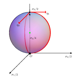
Figure 14: The GNO charge ${\mathds{Q}}=\sigma_{3}/2$ supports an unstable solution of the ${\rm SU}(2)$ YM theory over the two-sphere. Its $\nu=2$ negative modes are recovered as the tangents to the energy-reducing two-sphere whose top is ${\mathds{Q}}=\sigma_{3}/2$ is and whose bottom is the vacuum. The vertical axis is the Cartan algebra of ${\mathfrak{su}}(2)$.

Let us first consider loops. According to (8.224) our two-sphere of loops is

$$h_{\xi}(t)=e^{i\pi t\xi}e^{i\pi t\sigma_{3}},$$ (8.238)

where $\xi\in S=g^{-1}\sigma_{3}g$, $g\in{\rm SU}(2)$. Parametrizing ${\rm SU}(2)$ with Euler angles $(\tau,\varrho,\psi)$, $0\leq\tau\leq\pi,\,0\leq\varrho\leq 2\pi,\,0\leq\psi\leq 4\pi$,

$$g=e^{i\varrho\sigma_{3}/2}e^{i\tau\sigma_{2}/2}e^{i\psi\sigma_{3}/2}=\left(\begin{array}[]{cc}e^{i\frac{\varrho+\psi}{2}}\cos\frac{\tau}{2}&e^{i\frac{\varrho-\psi}{2}}\sin\frac{\tau}{2}\\[6.0pt] -e^{-i\frac{\varrho-\psi}{2}}\sin\frac{\tau}{2}&e^{-i\frac{\varrho+\psi}{2}}\cos\frac{\tau}{2}\end{array}\right),$$

yields the parametrization with polar angles $(\tau,\psi)$ of the $\xi$-sphere,

$$\xi=\left(\begin{array}[]{ll}\cos\tau&e^{-i\psi}\sin\tau\\[6.0pt] e^{i\psi}\sin\theta&-\cos\tau\end{array}\right)\in{\mathfrak{su}}(2)\,.$$

Then

$$e^{i\pi t\xi}=\left(\begin{array}[]{ll}\cos\pi t+i\sin\pi t\cos\tau&ie^{-i\psi}\sin\pi t\sin\tau\\[8.0pt] ie^{i\psi}\sin\pi t\sin\tau&\cos\pi t-i\sin\pi t\cos\tau\end{array}\right),\quad e^{i\pi t\sigma_{3}}=\left(\begin{array}[]{ll}e^{i\pi t}&0\\[8.0pt] 0&e^{-i\pi t}\end{array}\right)$$ (8.241)

so that our sphere of loops (8.238) reads

$$h_{\xi}(t)=\left(\begin{array}[]{cc}\left(\cos\pi t+i\sin\pi t\cos\tau\right)e^{i\pi t}&ie^{-i\left(\psi+\pi t\right)}\sin\pi t\sin\tau\\[12.0pt] ie^{i\left(\psi+\pi t\right)}\sin\pi t\sin\tau&\left(\cos\pi t-i\sin\pi t\cos\tau\right)e^{-i\pi t}\end{array}\right).$$ (8.244)

Calculating the speed of our loops,

$$h^{-1}{\partial}_{t}h=i\pi\left(\begin{array}[]{cc}1+\cos\tau&e^{-i(\psi+2\pi t)}\sin\tau\\[8.0pt] e^{i(\psi+2\pi t)}\sin\tau&-1-\cos\tau\end{array}\right),$$ (8.245)

[$h\equiv h_{\xi}$] allows us to infer that the energy of the loop with parameter $\xi$ is simply the height function on the unit $\xi$-sphere,

$$L^{(\tau,\psi)}=\pi(1+\cos\tau).$$ (8.246)

This result is also consistent with (8.228). The intuitive picture is that of Fig. 3 with the “sphere” meaning now ${\rm SU}(2)\approx{\mathds{S}}^{3}$.

In YM terms, (8.234) yields in turn the $2$-sphere of YM configurations reads

$$A_{\theta}^{\ \xi}=0,\;A_{\varphi}^{\ \xi} = \hbox{$\textstyle\frac{1}{4}$}(1-\cos\theta)\Big{\{}(1+\cos\tau)\sigma_{3}-\sin\tau(e^{-i(\varrho+\varphi)}\sigma_{+}+e^{i(\varrho+\varphi)}\sigma_{-})\Big{\}}$$

$$= \hbox{$\textstyle\frac{1}{4}$}(1-\cos\theta)\Big{\{}(1+\cos\tau)\sigma_{3}-\sin\tau\big{(}\cos(\varrho+\varphi)\sigma_{1}+\sin(\varrho+\varphi)\sigma_{2}\big{)}\Big{\}}\quad$$

in $N$, and similarly in $S$.

$\bullet$ For $\tau=0,\ \xi=\sigma_{3}$ and so we get ${\bm{A}}=(\sigma_{3}/2){\bm{A}}^{D}$ i.e. the monopole we started with.

$\bullet$ For $\tau=\pi,\ \xi=-\sigma_{3}$, and we get instead ${\bm{A}}=0$, the vacuum. The energy field strength tensor reads

$$F_{\theta\varphi}^{\xi}=\hbox{$\textstyle\frac{1}{4}$}\sin\theta\Big{\{}(1+\cos\tau)\sigma_{3}-\sin\tau\big{(}\cos(\varrho+\varphi)\sigma_{1}+\sin(\varrho+\varphi)\sigma_{2}\big{)}\Big{\}},$$ (8.248)

whose energy is

$$E^{(\tau,\psi)}=\pi(1+\cos\tau),$$ (8.249)

the same as the loop energy (8.246).

Higher charges support more instabilities. Fig.15 shows, for example, what happens for the GNO charge ${\mathds{Q}}=\sigma_{3}$, which has $\nu=6$ negative modes and sits at the top of $3$ energy-reducing two-spheres.

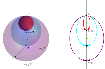
Figure 15: The ${\rm SU}(2)$ monopole with GNO charge $Q=\sigma_{3}$ has $\nu=6$ negative modes. It sits at the top of $3$ energy-reducing two-spheres whose bottoms are the lower-lying charges $\sigma_{3}/2,\,0$ and $-\sigma_{3}/2$.

Example 2: $H={\rm SO}(3)$

For $H={\rm SO}(3)$ the topologically trivial sector is the same as for $H={\rm SU}(2)$. Non-trivial topology arises for

$${\stackrel{{\scriptstyle{\,\raise 0.5pt\hbox{$\scriptstyle\circ$}\,}}}{{{\mathds{Q}}}}}{}^{(1)}=\frac{\sigma_{3}}{4},$$ (8.250)

which is the unique stable charge with $m=1\in{\mathds{Z}}_{2}$.

The ${\rm SO}(3)$ monopole with GNO charge

$${\mathds{Q}}=\frac{3}{4}\sigma_{3},$$ (8.251)

for example, is unstable. Its $\nu=2$ negative modes are tangent to the energy-reducing two-sphere

$$A_{\theta}^{\ \xi}=0\qquad{\left(A_{\varphi}^{\ \xi}\right)}_{\pm}=\hbox{$\textstyle\frac{1}{4}$}\displaystyle{(\pm 1-\cos\theta)}\big{(}e^{-i\varphi{\hbox{$\textstyle\frac{1}{2}$}}\sigma_{3}}\,\xi\,e^{i\varphi{\hbox{$\textstyle\frac{1}{2}$}}\sigma_{3}}+2\sigma_{3}\big{)},$$ (8.252)

which interpolates between ${\mathds{Q}}=\frac{3}{4}\sigma_{3}$ and the stable monopole with ${\stackrel{{\scriptstyle{\,\raise 0.5pt\hbox{$\scriptstyle\circ$}\,}}}{{{\mathds{Q}}}}}{}^{(1)}=\frac{1}{4}\sigma_{3}$, see Fig.16. This sphere is in fact obtained from (8.3) by shifting its bottom from the origin to ${\stackrel{{\scriptstyle{\,\raise 0.5pt\hbox{$\scriptstyle\circ$}\,}}}{{{\mathds{Q}}}}}{}^{(1)}=\sigma_{3}/4$.

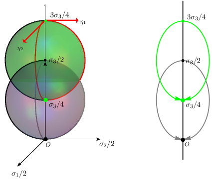
Figure 16: For $H={\rm SO}(3)$ the vacuum sector is that of ${\rm SU}(2)$. In the non-trivial $m=1\in{\mathds{Z}}_{2}$ sector the only stable monopole has GNO charge ${\stackrel{{\scriptstyle{\,\raise 0.5pt\hbox{$\scriptstyle\circ$}\,}}}{{{\mathds{Q}}}}}{}^{(1)}=\sigma_{3}/4$. The monopole with charge ${\mathds{Q}}=\frac{3}{4}\sigma_{3}$ is unstable with $\nu=2$ negative modes, which are tangent to the energy-reducing two-sphere whose top is ${\mathds{Q}}=\frac{3}{4}\sigma_{3}$ is and whose bottom is ${\stackrel{{\scriptstyle{\,\raise 0.5pt\hbox{$\scriptstyle\circ$}\,}}}{{{\mathds{Q}}}}}{}^{(1)}$.

Example 3: $H={\rm U}(2)$

The case $H={\rm U}(2)$ has already been studied in Section 3. The Bott diagram of ${\rm U}(2)$ is as on Fig.9. The horizontal lines are the topological sectors labelled by $m$. In each sector, the [up to conjugation unique] stable charge is the one which is the closest to the central ${\mathfrak{u}}(1)$, namely $2{\stackrel{{\scriptstyle{\,\raise 0.5pt\hbox{$\scriptstyle\circ$}\,}}}{{{\mathds{Q}}}}}{}^{(m)}={\stackrel{{\scriptstyle{\,\raise 0.5pt\hbox{$\scriptstyle\circ$}\,}}}{{Q}}}{}^{(m)}$ in (3.76).

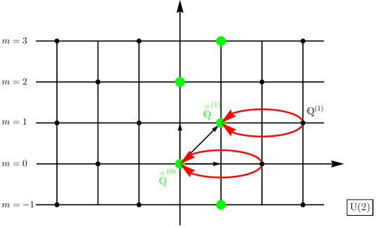
Figure 17: For ${\rm U}(2)$ the vacuum sector $m=0$ is that of ${\rm SU}(2)$ imbedded into of ${\rm U}(2)$. The $m=2k+1$ odd sector is obtained from that of $m=0$ by shifting the origin to ${\stackrel{{\scriptstyle{\,\raise 0.5pt\hbox{$\scriptstyle\circ$}\,}}}{{{\mathds{Q}}}}}{}^{(m)}=\frac{m}{4}\sigma_{3}$. Alternatively, it is identical to the $m=1\in{\mathds{Z}}_{2}$ sector of ${\rm SO}(3)$. For example, the monopole with charge ${\mathds{Q}}=\frac{1}{4}{\rm diag}(3,-1)$ lies in the $m=1$ sector and is unstable with Morse index $\nu=2$. An energy-reducing $2$-sphere links it to the stable monopole of the sector with GNO charge ${\stackrel{{\scriptstyle{\,\raise 0.5pt\hbox{$\scriptstyle\circ$}\,}}}{{{\mathds{Q}}}}}{}^{(1)}$.

Any other monopole charge of sector $m$ is

$${\mathds{Q}}^{(m)}={\hbox{$\textstyle\frac{1}{2}$}}{\stackrel{{\scriptstyle{\,\raise 0.5pt\hbox{$\scriptstyle\circ$}\,}}}{{Q}}}{}^{(m)}+\frac{n}{2}P_{1}={\hbox{$\textstyle\frac{1}{2}$}}{\stackrel{{\scriptstyle{\,\raise 0.5pt\hbox{$\scriptstyle\circ$}\,}}}{{Q}}}{}^{(m)}+\;\frac{1}{2}{\rm diag}(n,-n).$$

Those monopoles for which $n\neq 0$ are unstable with index $\nu=2(2n-1)$ for $m$ even, and $\nu=4n$ for $m$ odd (Fig. 17).

For example, when $G={\rm SU}(3)$ is broken to $H={\rm U}(2)$ by an adjoint Higgs $\Phi$ [54], the vacuum sector contains a configuration whose non-Abelian charge is [conjugate to]

$${\mathds{Q}}={\rm diag\ }({\hbox{$\textstyle\frac{1}{2}$}},-{\hbox{$\textstyle\frac{1}{2}$}},0),$$ (8.253)

where we considered $H={\rm U}(2)$ as imbedded into $G={\rm SU}(3)$. Note that (8.253) is precisely in the ${\rm SU}(2)$ monopole imbedded into the topologically trivial sector of ${\rm U}(2)$ considered in Example 1 and depicted on Fig.14. This configuration is therefore unstable as conjectured in [54], and has indeed $2$ negative modes, namely

$$a_{\theta}^{\pm}=e^{\mp i\varphi}\,\frac{\sigma_{\pm}}{2},\qquad a_{\varphi}^{\pm}=\mp e^{\mp i\varphi}\sin\theta\,\frac{\sigma_{\pm}}{2}\,.$$ (8.254)

tangent to the energy-reducing two-sphere (8.3).

Example 4: $H={\rm U}(3)$.

The physically most relevant example is when the Higgs little group is $H={\rm U}(3)$ i.e. locally ${\mathfrak{su}}(3)_{c}+{\mathfrak{u}}(1)_{em}$, the symmetry group of strong and electromagnetic interactions. The Bott diagram is shown on Fig. 12.

The topological sectors are labelled by an integer $m$; the unique stable charge in the $m$-sector is $2{{\stackrel{{\scriptstyle{\,\raise 0.5pt\hbox{$\scriptstyle\circ$}\,}}}{{{\mathds{Q}}}}}}{}^{(m)}={{\stackrel{{\scriptstyle{\,\raise 0.5pt\hbox{$\scriptstyle\circ$}\,}}}{{Q}}}}{}^{(m)}$ in (3.86). Any other monopole in the sector has charge

$$2{{\mathds{Q}}}^{(m)}={{\stackrel{{\scriptstyle{\,\raise 0.5pt\hbox{$\scriptstyle\circ$}\,}}}{{Q}}}}{}^{(m)}+Q^{\prime}={{\stackrel{{\scriptstyle{\,\raise 0.5pt\hbox{$\scriptstyle\circ$}\,}}}{{Q}}}}^{(m)}+n_{1}P_{1}+n_{2}P_{2}={{\stackrel{{\scriptstyle{\,\raise 0.5pt\hbox{$\scriptstyle\circ$}\,}}}{{Q}}}}{}^{(m)}+{\rm diag}(n_{1},n_{2}-n_{1},-n_{2}).$$ (8.255)

Those configurations with $Q^{\prime}\neq 0$ are unstable.

For example, the ${\mathds{Q}}={\rm diag}(1,0,-1)$ (Fig.18) belongs to the vacuum sector, because its charge is in $\mathfrak{k}={\mathfrak{su}}(3)$.

$$\alpha_{1}(2{\mathds{Q}})=2,\quad\alpha_{2}(2{\mathds{Q}})=2,\quad\theta(2{\mathds{Q}})=4,$$

and so there are $10$ negative modes, given by (5.163). Equation (8.224) yields in turn $5$ energy-reducing $2$-spheres, which end at

$${\mathds{Q}}_{\alpha_{1}}={\rm diag\ }(1,-1/2,-1/2),\qquad{\mathds{Q}}_{\alpha_{2}}={\rm diag\ }(1/2,1/2,-1),$$ (8.256)

$${\mathds{Q}}_{\theta}^{(1)}={\rm diag\ }(1/2,0,-1/2),\quad{\mathds{Q}}_{\theta}^{(2)}=0,\quad{\mathds{Q}}_{\theta}^{(3)}={\rm diag\ }(-1/2,0,1/2),$$

respectively.

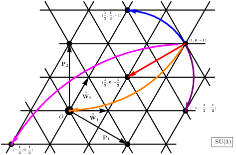
Figure 18: The $H={\rm SU}(3)$ monopole with GNO charge ${\mathds{Q}}={\rm diag}(1,0,-1)$ is unstable with 10 negative modes, tangent to $5$ energy-reducing spheres, which connect ${\mathds{Q}}$ to $5$ lower-energy monopoles.

Example 5: $H={\rm SU}(3)/{\mathds{Z}}_{3}$

In Ref. [55] the authors consider a $6$-dimensional pure ${\rm SU}(3)/{\mathds{Z}}_{3}$ Yang–Mills model, defined over $M^{4}\times{\mathds{S}}^{2}$, where $M^{4}$ is Minkowski space. They claim that any (Poincaré)$\times{\rm SO}(3)$ symmetric configuration is unstable against the formation of tachyons. This is not so, however; a counterexample is given by Forgács et al. [56], who show that the “symmetry-breaking vacuum”

$$A_{i}=0,\quad i=1,\dots 4,\qquad{\bm{A}}=\hbox{$\textstyle\frac{1}{6}$}\,{\rm diag}(2,-1,-1)\,{\bm{A}}^{D}$$ (8.257)

(where ${\bm{A}}$ is a $2$-vector on the extra-dimensional ${\mathds{S}}^{2}$), is indeed stable.

These observations have a simple explanation: the assumption of spherical symmetry in the extra dimensions leads to asymptotic monopole configurations on ${\mathds{S}}^{2}$ with gauge group $H={\rm SU}(3)/{\mathds{Z}}_{3}$. Since $\pi_{1}({\rm SU}(3)/{\mathds{Z}}_{3})\simeq{\mathds{Z}}_{3}$, there are three topological classes corresponding to the three central elements $z^{*}_{0}=1,\,z^{*}_{1}=e^{2\pi i/3},\,z^{*}_{2}=e^{4\pi i/3}$ of $H={\rm SU}(3)$ (Fig. 11).

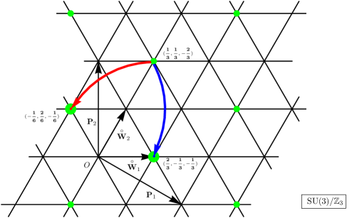
Figure 19: The YM theory on ${\mathds{S}}^{2}$ with gauge group $H={\rm SU}(3)/{\mathds{Z}}_{3})\simeq{\mathds{Z}}_{3}$ has $3$ topological sectors labelled by the central element $z_{a}\in Z$ of $SU(3)$. Each sector contains exactly one minimal charge ${\stackrel{{\scriptstyle{\,\raise 0.5pt\hbox{$\scriptstyle\circ$}\,}}}{{W}}}_{j},\ j=0,1,2,$ representing the [up to conjugation] only stable monopole of the sector. The one with charge $2{\mathds{Q}}=2{\stackrel{{\scriptstyle{\,\raise 0.5pt\hbox{$\scriptstyle\circ$}\,}}}{{W}}}_{2}={\rm diag}(1,-{\hbox{$\textstyle\frac{1}{2}$}},-{\hbox{$\textstyle\frac{1}{2}$}}),$ for example, belongs to the sector the sector labelled by $z_{1}=e^{4\pi i/3}$, and is unstable with $4$ independent negative modes. It lies at the top of two energy-reducing $2$-spheres whose bottoms are ${\stackrel{{\scriptstyle{\,\raise 0.5pt\hbox{$\scriptstyle\circ$}\,}}}{{W}}}_{1}$ and its conjugate.

The configuration (8.257) is indeed stable, because it is an [asymptotic] monopole with charge

$${\stackrel{{\scriptstyle{\,\raise 0.5pt\hbox{$\scriptstyle\circ$}\,}}}{{{\mathds{Q}}}}}={\hbox{$\textstyle\frac{1}{2}$}}{\stackrel{{\scriptstyle{\,\raise 0.5pt\hbox{$\scriptstyle\circ$}\,}}}{{W}}}_{1},$$ (8.258)

which is the unique stable charge of the Sector characterized by $z^{*}_{2}$.

On the other hand, any other configuration, e.g. [56]

$${\bm{A}}=\hbox{$\textstyle\frac{1}{3}$}{\rm diag}(1,1,-2)\,{\bm{A}}^{D}$$ (8.259)

is unstable. Counting the intersections with the root planes shows that there are $\nu=4$ negative modes.

Both configuration (8.257) and (8.259) belong to the same sector, and the construction of Sec. 7 provides us with two energy-reducing two-spheres from the monopole (8.259) to those with charges (8.257)) and its conjugate,

$$\hbox{$\textstyle\frac{1}{6}$}{\rm diag}(2,-1,-1)\qquad\hbox{and}\qquad\hbox{$\textstyle\frac{1}{6}$}{\rm diag}(-1,2,-1)$$ (8.260)

Choosing instead ${\stackrel{{\scriptstyle{\,\raise 0.5pt\hbox{$\scriptstyle\circ$}\,}}}{{{\mathds{Q}}}}}={\hbox{$\textstyle\frac{1}{2}$}}{\stackrel{{\scriptstyle{\,\raise 0.5pt\hbox{$\scriptstyle\circ$}\,}}}{{W}}}_{2}$ would obviously lead to another stable configuration.

Example 5: $H={\rm Spin}(5)\simeq{\rm SO}(5)$.

As a final example, let us consider $H={\rm SO}(5)$ in Example 5 of Section 3.

It may be worth noting that, in contrast to the $K={\rm SU}(N)$ case, ${\mathds{Q}}={\hbox{$\textstyle\frac{1}{2}$}}W_{1}$ is an unstable monopole in the vacuum sector which has index $2(\theta(W_{1})-1)=2$ .

The negative modes are expressed once more by (8.254), but this time $\sigma_{\pm}$ mean

$$\sigma_{+}={\hbox{$\textstyle\frac{1}{2}$}}\left(\begin{array}[]{cccc}0&1&&\\ 0&0&&\\ &&0&-1\\ &&0&0\end{array}\right),\qquad\sigma_{-}={\hbox{$\textstyle\frac{1}{2}$}}\left(\begin{array}[]{cccc}0&0&&\\ 1&0&&\\ &&0&0\\ &&-1&0\end{array}\right)\ .$$ (8.261)

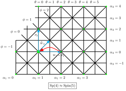
Figure 20: For ${\rm Spin}(5)$, the two co-weights are $W_{1}={\rm diag}(1,0,-1,0)$ and ${\stackrel{{\scriptstyle{\,\raise 0.5pt\hbox{$\scriptstyle\circ$}\,}}}{{W}}}_{2}={\rm diag}({\hbox{$\textstyle\frac{1}{2}$}},{\hbox{$\textstyle\frac{1}{2}$}},-{\hbox{$\textstyle\frac{1}{2}$}},-{\hbox{$\textstyle\frac{1}{2}$}})$ but only ${\stackrel{{\scriptstyle{\,\raise 0.5pt\hbox{$\scriptstyle\circ$}\,}}}{{W}}}_{2}$ is minimal. The monopole with charge ${\mathds{Q}}={\hbox{$\textstyle\frac{1}{2}$}}W_{1}$ is unstable with two negative modes. It lies on the top of an energy-reducing $2$-sphere which ends at the vacuum.

9 Conclusion

This review is devoted to the study of various aspects of “Brandt–Neri–Coleman” instability of monopoles . Our clue is to reduce the problem to pure YM theory on the “sphere at infinity” with the residual group $H$ as gauge group. Studying the Hessian we have proved the Theorem announced by Goddard an Olive [10], and by Coleman [3], which says that each topological sector admits a unique stable monopole whereas all other solutions of the YM equations are unstable with an even Morse index [=number of negative modes].

Turning to the global aspects, we have shown that to each such unstable monopole with Morse index $\nu=2n$ sits on the top of $n$ energy-reducing two-sphere whose bottom is some lower-energy monopole .

An unstable monopole should decay by radiating away its energy. Describing such a process would require solving the time-dependent YM(H) field equations with initial conditions close to a static solution cf. [58]. But this is beyond the reach of present technical knowledge.

An approximate approach would be to argue first that, under suitable conditions, a monopole can be considered a classical object which preserves its identity during the process; then radiation could act as a sort of effective potential.

Intuitively, our monopole could “roll down” to some lower-lying critical point, from which it would continue to “roll” further down as a sort of “cascade” until it ends up at the stable lowest-lying state. It is tempting to figure that our energy-reducing spheres could provide us with possible decay routes for an unstable monopole.

Realizing this picture in a physical framework is quite challenging an we have not been able to carry it out yet. All what we did so far has been to construct a sort “monopole landscape”: no dynamics has been considered.

Would like to hint at an analogy, namely that with monopole scattering following Manton’s ideas [48]. Remember first that the space of static self-dual monopoles of the Bogomolny–Prasad–Sommerfield type [2, 3, 28, 4, 6] form a finite dimensional submanifold called the moduli space, whose dimension is the number of independent zero modes. Every point in the moduli space labels such a solution which saturates the Bogomolny bound of the energy. All of them have therefore the same [namely the lowest possible] energy, determined by the topological charge.

Then the kinetic term in the Yang–Mills–Higgs action defines a metric on the moduli space, and slowly moving monopoles follow approximately geodesics [48, 51].

Intuitively, the moduli space is the horizontal “bottom” on Fig. 2, and monopole scattering corresponds to a point “rolling” along such a flat direction with no resistance.

Acknowledgments. The investigations presented in this review started quarter of a century ago [8, 9], and were revived at the occasion of a Lecture presented by one of us (PAH) at the meeting “Nonlinear phenomena: a view from mathematics and physics”, organized by the National Taiwan University and the Taida Institute for Mathematical Sciences. Taipei, Jan. 2011. We dedicate our paper to the memory of late L. O’Raifeartaigh in collaboration with whom some of the results presented here were obtained. P.A.H and P.M.Z are indebted to the Institute of Modern Physics of the Lanzhou branch of the Chinese Academy of Sciences and to the Laboratoire de Mathématiques et de Physique Théorique of Tours University for hospitality, respectively. This work has been partially supported by the National Natural Science Foundation of China (Grant No. 11035006) and by the Chinese Academy of Sciences visiting professorship for senior international scientists (Grant No. 2010TIJ06).

References

- [1] G. ’t Hooft, “Magnetic Monopoles in Unified Gauge Theories,” Nucl. Phys. B79, 276 (1974); A. M. Polyakov, “Particle Spectrum in the Quantum Field Theory,” JETP Lett. 20, 194 (1974)
- [2] P. Goddard and D. Olive, “New Developments in the Theory of Magnetic Monopoles,” Rep. Prog. Phys. 41 (1978) 1357
- [3] S. Coleman, “The magnetic monopole fifty years later,” in The Unity of Fundamental Interactions, ed. A. Zichichi (Plenum New York, 1983); Aspects of Symmetries. Selected Erice Lectures. Cambridge UP (1885).
- [4] P. A. Horváthy, Introduction to monopoles, Naples, Italy: Bibliopolis (1988). Monographs and Textbooks in Physical Science. Lecture Notes, 6.
- [5] N. Manton and P. Sutcliffe, Topological solitons, Cambridge Monographs on Mathematical Physics (2004) Book DOI: 10.1017/CBO9780511617034.
- [6] K. Konishi, “The magnetic monopoles seventy-five years later,” Lect. Notes Phys. 737 (2008) 471 [arXiv:hep-th/0702102].
- [7] R. A. Brandt and F. Neri, “Stability analysis for singular non-Abelian magnetic monopoles,” Nucl. Phys. B161 (1979) 253
- [8] P. A. Horváthy and J. H. Rawnsley, “On the stability of monopoles,” in Proceedings of the International Conference on Differential Geometric Methods in Theoretical Physics. Clausthal’1986. p.108 (World Scientific, Singapore); P. A. Horváthy, “Monopole geography,” Proc. Non-perturbative Methods in QFT, ed. Z. Horváth, L. Palla and A. Patkós. p.39. Singapore: World Scientific (1987).
- [9] P. A. Horváthy, L. O’Raifeartaigh and J. H. Rawnsley, “Monopole-charge instability”, Int. Journ. Mod. Physics A3 (1988) 665-702. Available as arXiv:0909.2523 [hep-th].
- [10] P. Goddard and D. I. Olive, “The magnetic charges of stable selfdual monopoles,” Nucl. Phys. B191 (1981) 528.
- [11] Th. Friedrich and L. Habermann, “Yang–Mills equations on the two-dimensional sphere,’ Commun. Math. Phys. 100 (1985) 231;
- [12] W. Nahm and K. Uhlenbeck, “The equivalence of quantized gauge fields on and the quantum mechanics of a particle moving on the group manifold.”. Unpublished notes, Chicago (1988).
- [13] J. Milnor, Morse Theory, Ann. Math. Studies 51. Princeton University Press, New Jersey (1963); R. Bott, Bull. Amer. Math. Soc. 7 (3) (1982) 331
- [14] J. Arafune, P. G. O. Freund and C. J. Goebel, “Topology of Higgs fields,” J. Math. Phys. 16 (1975) 433.
- [15] A. S. Schwarz, “Magnetic monopoles in gauge theories,” Nucl. Phys. B112, 358 (1976)
- [16] C. H. Taubes, “Surface integrals and monopole charges in non-Abelian gauge theories,” Commun. Math. Phys. 81, 299 (1981)
- [17] P. A. Horváthy and J. H. Rawnsley, “Topological charges in monopole theories” Commun. Math. Phys. 96 (1984) 497; “Monopole charges for arbitrary compact gauge groups and Higgs fields in any representation” Commun. Math. Phys. 99 (1985) 517; P. A. Horvathy and J. H. Rawnsley, “Monopole invariants,” J. Phys. A 20 (1987) 747. In a rather peculiar way, the same topological charge arises for non-topological “Jackiw-Pi” vortex solutions, see P. A. Horvathy, “Topology of non-topological Chern-Simons vortices,” Lett. Math. Phys. 49, 67 (1999).
- [18] E. Lubkin, “Geometric definition of gauge invariance,” Annals Phys. 23 (1963) 233.
- [19] P. Goddard, J. Nuyts, and D. Olive, “Gauge Theories and Magnetic Charge,” Nucl. Phys. B125 (1977) 1;
- [20] M. F. Atiyah and R. Bott, “The Yang–Mills equations over Riemann surfaces,” Philos. Trans. Roy. Soc. London Ser. A 308 (1983) 523.
- [21] J. M. Speight, “The ground state energy of a charged particle on a Riemann surface,” arXiv:1012.3337 [hep-th].
- [22] R. Bott, in Representation Theory of Lie Groups. Proc. Oxford’77, ed. Atiyah (Cambridge University Press, 1979) p. 63.
- [23] I. Singer, “The Geometry of the Orbit Space for Non-Abelian Gauge Theories.” Phys. Scripta 24 (1984) 817
- [24] N. S. Manton, “Topology in the Weinberg-Salam theory,” Phys. Rev. D28 (1983) 2019;
- [25] C. Taubes, “Stability in Yang–Mills theories,” Commun. Math. Phys. 91, 235 (1983).
- [26] P. Forgács and Z. Horváth, “Topology and saddle points in field theories,” Phys. Lett. 138B 397 (1984);
- [27] L. M. Sibner, J. Talvacchia, “The Existence of nonminimal solutions of the Yang-Mills Higgs equations over R**3 with arbitrary positive coupling constant,” Commun. Math. Phys. 162, 333-351 (1994).
- [28] E. B. Bogomolny, “Stability of classical solutions,” Sov. J. Nucl. Phys. 24 (1976) 449, M. K. Prasad and C. M. Sommerfield, “An exact classical solution for the ’t Hooft monopole and the Julia–Zee dyon,” Phys. Rev. Lett. 35 (1975) 760;
- [29] P. A. M. Dirac, “Quantized singularities in the electromagnetic field,” Proc. Roy. Soc. Lond. A 133 (1931) 60.
- [30] N. Steenrod, Topology of fibre bundles, Princeton Univ. Press (1951)
- [31] S. Kobayashi and K. Nomizu, Foundations of differential geometry, Vol. I N.Y. Interscience (1963); Vol. II N.Y. Interscience (1969)
- [32] R. Bott and L. Tu, Differential forms in algebraic topology. (Springer Verlag, New York, Heidelberg, Berlin 1982);
- [33] T. T. Wu and C. N. Yang, “Concept of nonintegrable phase factors and global formulation of gauge fields,” Phys. Rev. D 12, 3845 (1975).
- [34] T. T. Wu and C. N. Yang, “Dirac’s monopole without strings: Classical Lagrangian theory,” Phys. Rev. D 14 (1976) 437.
-
[35]
P. A. Horváthy,
“Classical action, the Wu-Yang phase factor and prequantization,”
Proc. Int. Coll. on Diff. Geom. Meths. in Math. Phys., Aix-en Provence ’79.
Ed. Souriau.
Springer Lecture Notes in Math. 836, 67 (1980). - [36] J. Sniatycki, “Prequantization of charge,” Journ. Math. Phys. 15, 619 (1974)
- [37] W. Greub and H. R. Petry, “Minimal coupling and complex line bundles,” Journ. Math. Phys. 16, 1347 (1975)
- [38] A. Trautman, “Solutions of the Maxwell and Yang-Mills Equations Associated with Hopf Fiberings,” Int.J.Theor.Phys. 16 561 (1977).
- [39] P. A. Horváthy, “Rotational Symmetry And Dirac’s Monopole,” Int. J. Theor. Phys. 20 (1981) 697.
- [40] A. Trautman, Differential geometry for physicists. Stony Brook lectures. Monographs and Textbooks in Physical Sciences. Bibliopolis: Napoli (1984).
- [41] A. Salam, “Weak And Electromagnetic Interactions,” In the Proceedings of 8th Nobel Symposium, Lerum, Sweden, 19-25 May 1968, pp. 367-377. ed. Alqvist and Wicksell, Stockholm (1968);
- [42] H. Georgi and S. L. Glashow, “Unified weak and electromagnetic interactions without neutral currents,” Phys. Rev. Lett. 28 (1972) 1494. “Partial Symmetries Of Weak Interactions,” Nucl. Phys. 22 (1961) 579.
-
[43]
Z. Horváth and L. Palla,
“Monopoles and Grand Unification Theories,”
Phys. Lett. B 69 (1977) 197;
“On the structure of generalized monopole solutions in gauge theories,”
Nucl. Phys. B 116 (1976) 500.
C. P. Dokos and T. N. Tomaras, “Monopoles and dyons in the SU(5) model,” Phys. Rev. D 21 (1980) 2940. - [44] J.E. Humphreys, Introduction to Lie Algebras and Representation Theory. (Berlin, Springer Verlag 1972).
- [45] P. A. Horváthy and J. H. Rawnsley: “Internal symmetries of non-Abelian gauge field configurations.” Phys. Rev. D32, 968 (1985).
- [46] P. Goddard and D. I. Olive, “Charge quantization in theories with an adjoint representation Higgs mechanism,” Nucl. Phys. B 191 (1981) 511;
- [47] T. T. Wu and C. N. Yang, “Dirac monopole without strings: monopole harmonics,” Nucl. Phys. B107 (1976) 365;
-
[48]
N. S. Manton,
“A remark on the scattering of BPS monopoles,”
Phys. Lett. B 110 (1982) 54;
“Monopole interactions at long range,”
Phys. Lett. B 154 (1985) 397
[Erratum-ibid. 157B (1985) 475].
M. F. Atiyah and N. J. Hitchin, “Low-energy scattering of non-Abelian magnetic monopoles,” Phil. Trans. Roy. Soc. Lond. A 315 (1985) 459.
M. F. Atiyah and N. J. Hitchin, “Low-Energy Scattering Of Non-abelian Monopoles,” Phys. Lett. A 107 (1985) 21.
M. F. Atiyah and N. J. Hitchin, “The geometry and dynamics of magnetic monopoles.” M. B. Porter Lectures. Princeton, USA, Univ. Press (1988). - [49] M. Spiegelglass, “Supersymmetric quantum mechanics on the sphere,” Phys. Lett. 166B (1986) 160.
- [50] L. Fehér, P. A. Horváthy, and L. O’Raifeartaigh, “Applications of chiral supersymmetry for spin fields in self-dual backgrounds.” Int. J. Mod. Phys. A4 5277 (1989).
-
[51]
E. J. Weinberg and P. Yi,
“Magnetic monopole dynamics, supersymmetry, and duality,”
Phys. Rept. 438 (2007) 65
[arXiv:hep-th/0609055];
E. J. de Vries and B. J. Schroers, “Supersymmetric Quantum Mechanics of Magnetic Monopoles: A Case Study,” Nucl. Phys. B 815 (2009) 368 [arXiv:0811.2155 [hep-th]]. - [52] P. A. Horváthy, “Extended Feynman formula for harmonic oscillator.” Int. Journ. Theor. Phys. 18, 245 (1979); “The Maslov correction in the semiclassical Feynman integral.” C. Eur. J. Phys. 9 (2011) 1 [quant-ph/0702236].
- [53] P. Forgács and N. S. Manton, “Space-time symmetries in gauge theories,” Commun. Math. Phys. 72, 15 (1980).
- [54] E. Corrigan, D. Olive, D. B. Fairlie J. Nuyts, “Magnetic monopoles in SU(3) gauge theories” Nucl. Phys. B106 (1976) 475.
- [55] S. Randjbar-Daemi, A. Salam and J. Strathdee, “Instability of higher dimensional Yang–Mills systems,” Phys. Lett. 124B (1983) 345;
- [56] P. Forgács, Z. Horváth and L. Palla, “Stable compactifying Einstein Yang–Mills systems,” Phys. Lett. 147B (1984) 311
- [57] F. A. Bais, “To be or not to be? Magnetic monopoles in non-Abelian gauge theories,” In *’t Hooft, G. (ed.): 50 years of Yang-Mills theory* pp. 271-307. [hep-th/0407197].
- [58] H. Guo and E. J. Weinberg, “Instabilities of chromodyons in SO(5) gauge theory,” Phys. Rev. D 77 (2008) 105026 [arXiv:0803.0736 [hep-th]].