A Unifying Statistical Model for Atmospheric Optical Scintillation

Abstract

In this paper we develop a new statistical model for the irradiance fluctuations of an unbounded optical wavefront (plane and spherical waves) propagating through a turbulent medium under all irradiance fluctuation conditions in homogeneous, isotropic turbulence. The major advantage of the model is that leads to closed-form and mathematically-tractable expressions for the fundamental channel statistics of an unbounded optical wavefront under all turbulent regimes. Furthermore, it unifies most of the proposed statistical models for the irradiance fluctuations derived in the bibliography providing, in addition, an excellent agreement with the experimental data.

I Introduction

Atmospheric optical communication is receiving considerable attention recently for use in high data rate wireless links. However, even in clear sky conditions, wireless optical links experience fluctuations in both the intensity and the phase of an optical wave propagating through this medium [1] due to time varying inhomogeneities in the refractive index of the atmosphere. The reliability of an optical system operating in such environment can be deduced from a mathematical model for the probability density function (pdf) of the randomly fading irradiance signal (scintillation). For that reason, one of the goals in studying optical wave propagation through turbulence is the identification of a tractable pdf of the irradiance under all intensity fluctuation regimes.

Over the years, many irradiance pdf models have been proposed with different degrees of success. Perhaps the most successful models are the log-normal [2], the lognormal-Rician (or Beckmann model) [3] and the gamma-gamma [4]. The scope of the lognormal model is restricted under weak irradiance fluctuations. The Beckmann model, although shows excellent agreement with experimental data, however a closed-form solution for its integral is unknown in addition to its inherent poor convergence properties. Finally, the gamma-gamma pdf was suggested as a reasonable alternative to Beckmann’s pdf because of its much more tractable mathematical model.

Now, through this paper, we propose a new and generic propagation model and, from it, we obtain a new and unifying statistical model for the irradiance fluctuations. The proposed model is valid under all range of turbulence conditions (weak to strong) and it is found to provide an excellent fit to experimental data. Furthermore, the statistical model presented here can be written in a closed-form expression and it contains most of the statistical models for the irradiance fluctuations that have been proposed in the bibliography. Thus, the utility of our model can be extended to many other areas of application as the study of fading in radiofrequency channels.

II The proposed model of propagation

Assume an electromagnetic wave is propagating through a turbulent atmosphere with a random refractive index. As the wave passes through this medium, part of the energy is scattered and the form of the irradiance probability distribution is determined by the type of scattering involved. In the physical model we present in this paper, the observed field at the receiver is supposed to consist of three terms: the first one is the line-of-sight (LOS) contribution, $U_{L}$, the second one is the component which is quasi-forward scattered by the eddies on the propagation axis, $U_{S}^{C}$, and coupled to the LOS contribution; whereas the third term, $U_{S}^{G}$, is due to energy which is scattered to the receiver by off-axis eddies, this latter contribution being statistically independent from the previous two other terms. The inclusion of this coupled to the LOS scattering component is the main novelty of the model and it can be justified by the high directivity and the narrow beamwidths of laser beams in atmospheric optical communications. The model description is depicted in Fig. 1.

Accordingly, we can write the total observed field as:

$$\begin{split}U=&\Bigl{(}U_{L}+U_{S}^{C}+U_{S}^{G}\Bigr{)}\exp{(\chi+jS)}\end{split}$$ (1)

where $U_{L}=\sqrt{G}\sqrt{\Omega}\exp{(j\phi_{A})}$, $U_{S}^{C}=\sqrt{G}\sqrt{\rho 2b_{0}}\exp{(j\phi_{B})}$ and $U_{S}^{G}$=$\sqrt{(1-\rho)}U^{\prime}_{S}$, being $U_{S}^{C}$ and $U_{S}^{G}$ statistically independent stationary random processes. Of course, $U_{L}$ and $U_{S}^{G}$ are also independent random processes. In (1), $G$ is a real variable following a gamma distribution with $E[G]$=$1$. It represents the slow fluctuation of the LOS component. Following [5], the parameter $\Omega$=$E[|U_{L}|^{2}]$ represents the average power of the LOS term whereas the average power of the total scatter components is denoted by $2b_{0}$ = $E[|U_{S}^{C}|^{2}$+$|U_{S}^{G}|^{2}]$. $\phi_{A}$ and $\phi_{B}$ are the deterministic phases of the LOS and the coupled-to-LOS scatter terms, respectively. On another note, $0$$\leq$$\rho$$\leq$$1$ is the factor expressing the amount of scattering power coupled to the LOS component. Finally, $U^{\prime}_{S}$ is a circular Gaussian complex random variable, and $\chi$ and $S$ are real random variables representing the log-amplitude and phase perturbation of the field induced by the atmospheric turbulence, respectively. A plausible justification for the coupled-to-LOS scattering component, $U_{S}^{C}$, is given in [6].

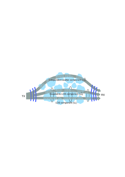
Figure 1: Proposed propagation geometry for a laser beam.

III Málaga (${\rm{}}{\cal M}$) probability density function

From Eq. (1), the observed irradiance of the proposed propagation model can be expressed as:

$$\begin{array}[]{l}{\rm{\emph{I}}}=\Bigl{|}U_{L}+U_{S}^{C}+U_{S}^{G}\Bigr{|}^{2}\exp{(2\chi)}=YX,\\ \left\{\begin{array}[]{l}Y\buildrel\Delta\over{=}\Bigl{|}U_{L}+U_{S}^{C}+U_{S}^{G}\Bigr{|}^{2}\hskip 1.42271pt({\hbox{small-scale fluctuations}})\\ X\buildrel\Delta\over{=}\exp{(2\chi)}\hskip 41.25641pt({\hbox{large-scale fluctuations}}),\\ \end{array}\right.\end{array}$$ (2)

where the small-scale fluctuations denotes the contributions to scintillation associated with turbulent cells smaller than either the first Fresnel zone or the transverse spatial coherence radius, whichever is smallest. In contrast, large-scale fluctuations of the irradiance are generated by turbulent cells larger than that of either the Fresnel zone or the so-called “scattering disk”, whichever is largest. From Eq. $\eqref{EqCampoDistribucionM}$, we can rewrite the lowpass-equivalent complex envelope as:

$$\begin{split}R(t)=&\Bigl{(}U_{L}+U_{S}^{C}+U_{S}^{G}\Bigr{)}=\sqrt{G}\Bigl{[}\sqrt{\Omega}\exp{(j\phi_{A})}\\ &\hskip 28.45274pt+\sqrt{\rho}\sqrt{2b_{0}}\exp{(j\phi_{B})}\Bigr{]}+\sqrt{(1-\rho)}U^{\prime}_{S},\end{split}$$ (3)

so that we have the identical shadowed Rice single model employed in [5], composed by the sum of a Rayleigh random phasor (the independent scatter component, $U^{\prime}_{S}$) and a Nakagami distribution, $\sqrt{G}$. Then, we can apply the same procedure exposed in [5] consisting in calculating the expectation of the Rayleigh component with respect to the Nakagami distribution and then deriving the pdf of the instantaneous power. Hence, the pdf of $Y$ is given by:

$$\begin{split}f_{Y}\left(y\right)=\frac{1}{{\gamma}}\left[{\frac{{\gamma\beta}}{{\gamma\beta+\Omega^{{}^{\prime}}}}}\right]^{\beta}\exp\left[{-\frac{y}{{\gamma}}}\right]~{}_{1}F_{1}\left({\beta;1;\frac{1}{{\gamma}}\frac{\Omega^{{}^{\prime}}}{{\left({\gamma\beta+\Omega^{{}^{\prime}}}\right)}}y}\right)\end{split}$$ (4)

where $\beta\buildrel\Delta\over{=}(E[G])^{2}/$Var$[G]$ is the amount of fading parameter with Var[$\cdot$] as the variance operator, being $|\cdot|$ the absolute value. We have denoted $\gamma=2b_{0}(1-\rho)$ and $\Omega^{{}^{\prime}}=\Omega+\rho 2b_{0}+2\sqrt{2b_{0}\Omega\rho}\cos{(\phi_{A}-\phi_{B})}$. Finally, $~{}_{1}F_{1}\left(a;c;x\right)$ is the Kummer confluent hypergeometric function of the first kind.

Otherwise, the large-scale fluctuations, $X\buildrel\Delta\over{=}\exp{(2\chi)}$, is widely accepted to be a lognormal amplitude [3] but, as in [4, 5], this distribution is approximated by a gamma one, this latter with a more favorable analytical structure. Then:

$$\begin{split}f_{X}\left(x\right)=\frac{{\alpha^{\alpha}}}{{\Gamma\left(\alpha\right)}}x^{\alpha-1}\exp\left({-\alpha x}\right),\end{split}$$ (5)

where $\alpha$ is a positive parameter related to the effective number of large-scale cells of the scattering process, as in [4].

Now, the statistical characterization of $I$ can be obtained. It is said that $I$ follows a ${\rm{}}{\cal M}$ distribution if $X$ and $Y$ are random variable distributions according to Eqs. $\eqref{EqPDFX}$ and $\eqref{EqPDFY2}$, respectively, with $\beta$ being a natural number (a generalized expression for $\beta$ being a real number can be also derived, with an infinite summation, but it is less interesting due to the high degree of freedom of the proposed distribution). Then, the pdf is represented by:

$$\begin{split}f_{I}\left(I\right)=A\sum\limits_{k=1}^{\beta}{a_{k}I^{\frac{{\alpha+k}}{2}-1}K_{\alpha-k}\left({2\sqrt{\frac{{\alpha\beta I}}{{\gamma\beta+\Omega^{\prime}}}}}~{}\right)}\end{split}$$ (6)

where

$$\left\{\begin{split}&A\buildrel\Delta\over{=}\frac{{2\alpha^{\frac{\alpha}{2}}}}{{\gamma^{1+{\alpha\over 2}}\Gamma\left(\alpha\right)}}\left({\frac{{\gamma\beta}}{{\gamma\beta+\Omega^{{}^{\prime}}}}}\right)^{\beta+\frac{\alpha}{2}};\\ &a_{k}\buildrel\Delta\over{=}\left({\begin{array}[]{*{20}c}{\beta-1}\\ {k-1}\\ \end{array}}\right){\left({\gamma\beta+\Omega^{{}^{\prime}}}\right)^{1-\frac{k}{2}}\over\left(k-1\right)!}\left({\Omega^{{}^{\prime}}\over\gamma}\right)^{k-1}\left({\frac{\alpha}{\beta}}\right)^{\frac{k}{2}}.\end{split}\right.$$ (7)

In Eq. (6), $K_{\nu}(\cdot)$ is the modified Bessel function of the second kind and order $\nu$. In the interest of clarity, the algebraic manipulation to prove this result is moved to Appendix A.

Finally, the $k^{th}$ centered moments of the irradiance signal following a ${\rm{}}{\cal M}$ distribution, denoted by $m_{k}\left(I\right)$, are given by:

$$\begin{split}m_{k}\left(I\right)\buildrel\Delta\over{=}E\left[{I^{k}}\right]=\frac{{\Gamma\left({\alpha+k}\right)}}{{\Gamma\left(\alpha\right)\alpha^{k}}}\frac{1}{\gamma}\left({\frac{{\gamma\beta}}{{\gamma\beta+\Omega^{{}^{\prime}}}}}\right)^{\beta}~{}\\ \times\sum\limits_{r=0}^{\beta-1}{\beta-1\choose r}\frac{1}{{r!}}\left({\frac{{\Omega^{{}^{\prime}}}}{{\gamma\left({\gamma\beta+\Omega^{{}^{\prime}}}\right)}}}\right)^{r}\frac{{\Gamma\left({k+r+1}\right)}}{{\left({\frac{\beta}{{\gamma\beta+\Omega^{{}^{\prime}}}}}\right)^{k+r+1}}}.\end{split}$$ (8)

The proof of this result is, again, moved to Appendix B.

To conclude this section, we attach in Table I a list of most of the existing distribution models for atmospheric optical communications and how they can be generated from the ${\rm{}}{\cal M}$ distribution model proposed here. The analytical expression for the different distribution models include in Table I can be consulted in the references provided next to their names.

TABLE I: Generation of different statistical models from the proposed ${\rm{}}{\cal M}$ distribution model.

Distribution model	Generation
Rice-Nakagami [1]	$\rho=0$
	Var$[|U_{L}|]=0$
	$\rho=0$
Lognormal [1, 7]	Var$[|U_{L}|]=0$
	$\gamma\rightarrow 0$
Gamma [4]	$\rho=0$
	$\gamma=0$
Shadowed-Rician distribution [5]	Var$[|X|]=0$
K distribution[4, 8]	$\Omega=0$ and $\rho=0$
	or $\beta=1$
	$\Omega=0$
HK (Homodyned K) distribution [8]	$\rho=0$
	$X=\gamma$
	$\Omega=0$
Exponential distribution [4]	$\rho=0$
	$\alpha\rightarrow\infty$
Gamma-gamma [4]	$\rho=1$, then $\gamma=0$
distribution	$\Omega^{{}^{\prime}}=1$
Gamma-Rician distribution [3]	$\beta\rightarrow\infty$

IV Comparison with experimental data

In this section, we compare the ${\rm{}}{\cal M}$ distribution model with some of the published numerical simulation data plots in [9] and [10] of the log-irradiance pdf, covering a range of conditions that extends from weak irradiance fluctuations far into the saturation regime. It is remarkable the evident analytical tractability by directly employing Eq. (6), with a finite summation of $\beta$ terms. Some results are shown in Fig. 2 emphasizing its extremely high accuracy. Thus, we plot in Figs. 2 (a)-(c) the predicted log-irradiance pdf associated with the ${\rm{}}{\cal M}$ distribution (black solid line) for comparison with some of the simulation data illustrated in Figs. 4, 5 and 7 of [9]. The simulation pdf values are plotted as a function of $(\ln I-<\ln I>)/\sigma$, as in [9], where $<\ln I>$ is the mean value of the log-irradiance and $\sigma=\sqrt{\sigma_{\ln I}^{2}}$, the latter being the root mean square (rms) value of $\ln I$. For sake of brevity, and as representative of typical atmospheric propagation, we only use the inner scale value $l_{0}=0.5R_{F}$ so we can include the effect of $l_{0}$ in our results, where the quantity $R_{F}$ is the scale size of the Fresnel zone. We also plot the gamma-gamma pdf (red dashed line) obtained in [4] for the sake of comparison. In Fig. 2 (a) we use a Rytov variance $\sigma_{1}^{2}=0.1$ corresponding to weak irradiance fluctuations, in Fig. 2 (b) we employ $\sigma_{1}^{2}=2$ corresponding to a regime of moderate irradiance fluctuations whereas in Fig. 2 (c), $\sigma_{1}^{2}$ was established to $25$ for a particular case of strong irradiance fluctuations. Values of the scaling parameter $\sigma$ required in the plots for the ${\rm{}}{\cal M}$ pdf are obtained from Andrews’ development [4] in the presence of inner scale.

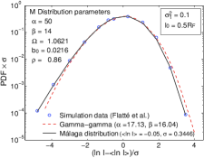
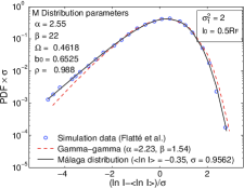
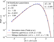
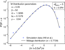
Figure 2: The pdf of the scaled log-irradiance for a plane wave (Figures (a), (b) and (c)) and a spherical wave (Figure (d)) in the case of: (a) weak irradiance fluctuations ($\sigma_{1}^{2}=0.1$ and $l_{0}/R_{F}=0.5$); (b) moderate irradiance fluctuations ($\sigma_{1}^{2}=2$ and $l_{0}/R_{F}=0.5$); (c) strong irradiance fluctuations ($\sigma_{1}^{2}=25$ and $l_{0}/R_{F}=0.5$); and (d) strong irradiance fluctuations ($\sigma_{Rytov}^{2}=5$ and $l_{0}/R_{F}=0.5$). The blue open circles represent simulation data, the dashed red line is from the gamma-gamma pdf with $\alpha$ and $\beta$ predicted in [9] and the solid black line is from our ${\rm{}}{\cal M}$ distribution model.

Finally, in Fig. 2 (d) we have obtained a very good fitting to the simulation data for a spherical wave in the case of strong irradiance fluctuations. Following Hill’s representation [10], the simulation pdf data and pdf values predicted by the ${\rm{}}{\cal M}$ distribution are displayed as a function of $(\ln I+0.5\sigma^{2})/\sigma$, where $\sigma$ was defined above. In this particular case of propagating a spherical wave, an additional parameter is needed: the Rytov parameter, $\sigma_{Rytov}^{2}$, defined as the weak fluctuation scintillation index in the presence of a finite inner scale.

For the particular case displayed in Fig. 2 (d), the gamma-gamma pdf does not fit with the simulation data and, even more, the Beckmann pdf did not lend itself directly to numerical calculations and so are omitted. Nevertheless, the ${\rm{}}{\cal M}$ pdf shows very good agreement with the data once again, with the advantage of a simple functional form, emphasized by the fact that its $\beta$ parameter is a natural number, which leads to a closed-form representation.

V Concluding remarks

In this paper, a novel statistical model for atmospheric optical scintillation is presented. Unlike other models, our proposal appears to be applicable for plane and spherical waves under all conditions of turbulence from weak to super strong in the saturation regime. The proposed model unifies in a closed-form expression the existing models suggested in the bibliography for atmospheric optical communications (see Table I). In addition to the mathematical expressions and developments, we have introduced a different perturbational propagation model that gives a physical sense to such existing models. Hence, the received optical intensity is due to three different contributions: first, a line of sight component, second, a coupled-to-LOS scattering component, as a remarkable novelty in the model, that includes the fraction of power traveling very closed to the line of sight, and eventually suffering from almost the same random refractive index variations than the LOS component; and third, the scattering component affected by refractive index fluctuations completely different to the other two components. The first two components are governed by a gamma distribution whereas the scattering component is depending on a circular Gaussian complex random variable. All of them let us model the amplitude of the irradiance (small-scale fluctuations), while the multiplicative perturbation that represents the large-scale fluctuations is approximated to follow a gamma distribution.

Finally, we have made a number of comparisons with published plane wave and spherical wave simulation data over a wide range of turbulence conditions (weak to strong) that includes inner scale effects. The ${\rm{}}{\cal M}$ distribution model is found to provide an excellent fit to the simulation data in all cases tested making computations extremely easy due to its closed-form expression.

Appendix A: proof of Equation (6)

To prove Eq. (6), we can obtain the Laplace transform, ${\rm{}}{\cal L}[f_{Y}\left(y\right);s]$, of the shadowed Rice single pdf, $f_{Y}(y)$, written in Eq. (4), in a direct way, with the help of Eq. (7) of Ref. [5], since the moment generating function (MGF) and the Laplace transform of the pdf $f_{Y}(y)$ are related by $M[f_{Y}(y);-s]={\rm{}}{\cal L}[f_{Y}(y);s]$:

$$\begin{split}{\rm{}}{\cal L}[f_{Y}\left(y\right);s]=\left({\frac{{\gamma\beta}}{{\gamma\beta+\Omega^{{}^{\prime}}}}}\right)^{\beta}\frac{{\left({1+\gamma s}\right)^{\beta-1}}}{{\left({\frac{{\gamma\beta}}{{\gamma\beta+\Omega^{{}^{\prime}}}}+\gamma s}\right)^{\beta}}}=\\ =\frac{1}{\gamma}\left({\frac{{\gamma\beta}}{{\gamma\beta+\Omega^{{}^{\prime}}}}}\right)^{\beta}\frac{{\left({\frac{1}{\gamma}+s}\right)^{\beta-1}}}{{\left({\frac{\beta}{{\gamma\beta+\Omega^{{}^{\prime}}}}+s}\right)^{\beta}}}.\end{split}$$ (9)

Now, let us consider the following Laplace-transform pair

$$\begin{split}\Gamma\left({\nu{\rm{+1}}}\right)\left({s-\lambda}\right)^{n}\left({s-\mu}\right)^{-\nu-1}\Leftrightarrow n!t^{\nu-n}e^{\mu t}L_{n}^{\nu-n}\left[{\left({\lambda-\mu}\right)t}\right],\\ {\mathop{\rm Re}\nolimits}(\nu)>n-1;\end{split}$$ (10)

given in [11], Eq. (4) in pp. 238, where the minor error in the sign of the argument of the Laguerre polynomial found and corrected in [12] has already taken into account. If we denote $\lambda=-\frac{1}{\gamma}$, $\mu=-\frac{\beta}{{\gamma\beta+\Omega^{{}^{\prime}}}}$, $n=\beta-1$ and $\nu=\beta-1$, then

$$\begin{split}\left({\beta-1}\right)!\left({s+\frac{1}{\gamma}}\right)^{\beta-1}\left({s+\frac{\beta}{{\gamma\beta+\Omega^{{}^{\prime}}}}}\right)^{-\beta}\Leftrightarrow\\ \Leftrightarrow\left({\beta-1}\right)!e^{-\frac{\beta}{{\gamma\beta+\Omega^{{}^{\prime}}}}t}L_{\beta-1}\left[{\frac{{-\Omega^{{}^{\prime}}}}{{\gamma\beta+\Omega^{{}^{\prime}}}}\frac{t}{\gamma}}\right],\end{split}$$ (11)

where $L_{n}[\cdot]$ is the Laguerre polynomial of order $n$. If we substitute Eq. (11) into Eq. (9), then the pdf of $Y$ can be expressed as:

$$\begin{split}f_{Y}\left(y\right)=\frac{1}{\gamma}\left({\frac{{\gamma\beta}}{{\gamma\beta+\Omega^{{}^{\prime}}}}}\right)^{\beta}\exp{\left(-\frac{\beta}{{\gamma\beta+\Omega^{{}^{\prime}}}}y\right)}\\ \times L_{\beta-1}\left[{\frac{{-\Omega^{{}^{\prime}}y}}{\left({\gamma\beta+\Omega^{{}^{\prime}}}\right)\gamma}}\right].\end{split}$$ (12)

Now, to obtain the unconditional ${\rm{}}{\cal M}$ distribution, from Eqs. (5) and (12), we can form:

$$\begin{split}f_{I}(I)&=\int_{0}^{\infty}{f_{Y}(I|x)f_{X}(x)\hbox{d}x}=\frac{{\alpha^{\alpha}}}{{\Gamma\left(\alpha\right)}}\frac{1}{\gamma}\\ &\times\left({\frac{{\gamma\beta}}{{\gamma\beta+\Omega^{{}^{\prime}}}}}\right)^{\beta}\int_{0}^{\infty}{\frac{1}{x}\exp{\left(-\frac{\beta}{{\gamma\beta+\Omega^{{}^{\prime}}}}\frac{I}{x}\right)}}\\ &\times{L_{\beta-1}\left[{\frac{-\Omega^{{}^{\prime}}}{{\gamma\beta+\Omega^{{}^{\prime}}}}\frac{I}{{\gamma x}}}\right]x^{\alpha-1}\exp\left({-\alpha x}\right)dx}.\end{split}$$ (13)

By expressing the Laguerre polynomial in a series,

$$\begin{split}L_{n}\left[x\right]=\sum\limits_{k=0}^{n}{(-1)^{k}\left({\begin{array}[]{*{20}c}n\\ k\\ \end{array}}\right)}\frac{{x^{k}}}{{k!}},\end{split}$$ (14)

as was shown in Eq. (8.970-1) of Ref. [13], and using Eq. (3.471-9) of Ref. [13], it follows that Eq. (13) becomes

$$\begin{split}f_{I}\left(I\right)=&\frac{{2\alpha^{\frac{\alpha}{2}}}}{{\Gamma\left(\alpha\right)}}\frac{1}{{\gamma^{1+\frac{\alpha}{2}}}}\left({\frac{{\gamma\beta}}{{\gamma\beta+\Omega^{{}^{\prime}}}}}\right)^{\beta}\left({\frac{{\gamma\beta}}{{\gamma\beta+\Omega^{{}^{\prime}}}}}\right)^{\frac{\alpha}{2}}\\ &\times\sum\limits_{k=1}^{\beta}{\left({\begin{array}[]{*{20}c}{\beta-1}\\ {k-1}\\ \end{array}}\right)}\frac{1}{{k-1!}}\left({\frac{{\Omega^{{}^{\prime}}}}{{\gamma\left(\gamma\beta+\Omega^{{}^{\prime}}\right)}}}\right)^{k-1}\\ &\times\left({\frac{\beta}{{\alpha\left({\gamma\beta+\Omega^{{}^{\prime}}}\right)}}}\right)^{-\frac{k}{2}}I^{\frac{{\alpha+k}}{2}-1}K_{\alpha-k}\left({2\sqrt{\frac{{\alpha\beta I}}{{\gamma\beta+\Omega^{{}^{\prime}}}}}}\right).\end{split}$$ (15)

Finally, Eq. (15) can be rewritten as Eq. (6), as was already anticipated in Section III.

Appendix B: proof of Equation (8)

From Eq. (2), the observed irradiance, $I$, of our proposed propagation model can be expressed as: $I=XY$, where the pdf of variables $X$ and $Y$ were written in Eqs. (5) and (4), respectively. Based on assumptions of statistical independence for the underlying random processes, $X$ and $Y$, then:

$$\begin{split}m_{k}\left(I\right)=E\left[{X^{k}}\right]E\left[{Y^{k}}\right]=m_{k}\left(X\right)m_{k}\left(Y\right).\end{split}$$ (16)

From Eq. (2.23) of Ref. [14], the moment of a Nakagami-m pdf is given by:

$$\begin{split}m_{k}\left(X\right)=\frac{{\Gamma\left({\alpha+k}\right)}}{{\Gamma\left(\alpha\right)\alpha^{k}}}.\end{split}$$ (17)

On the other hand, from Eqs. (12) and (14), and employing Eq. (3.381-4) of Ref. [13], obtain the moment of the Rician-shadowed distribution, given by:

$$\begin{split}m_{k}\left(Y\right)=&\frac{1}{\gamma}\left({\frac{{\gamma\beta}}{{\gamma\beta+\Omega^{{}^{\prime}}}}}\right)^{\beta}\sum\limits_{r=0}^{\beta-1}{\left({\begin{array}[]{*{20}c}{\beta-1}\\ r\\ \end{array}}\right)}\frac{1}{{r!}}\\ &\times\left({\frac{\Omega^{{}^{\prime}}}{{\gamma\left({\gamma\beta+\Omega^{{}^{\prime}}}\right)}}}\right)^{r}\frac{{\Gamma\left({k+r+1}\right)}}{{\left({\frac{\beta}{{\gamma\beta+\Omega^{{}^{\prime}}}}}\right)^{k+r+1}}}.\end{split}$$ (18)

Finally, when performing the product of Eq. (17) by Eq. (18), we certainly obtain Eq. (8).

References

- [1] L. C. Andrews and R. L. Phillips, Laser Beam Propagation Through Random Media. Bellingham, Washington, 1998.
- [2] X. Zhu and J.M. Kahn, “Free-space optical communication through atmospheric turbulence channels,” IEEE Trans. on Communications, vol.50, no.8, pp. 1293 – 1300, Aug 2002
- [3] J. H. Churnside and S.F. Clifford, “Log-normal Rician probability-density function of optical scintillations in the turbulent atmosphere,” J. Opt. Soc. Am. A, vol. 4, no. 10, pp. 1923–1930, Oct. 1987.
- [4] M.A. Al-Habash, L.C. Andrews and R.L. Phillips, “Mathematical model for the irradiance probability density function of a laser beam propagating through turbulent media,” Opt. Engineering, vol. 40, no. 8, pp. 1554–1562, Aug. 2001.
- [5] A. Abdi, W.C. Lau, M.-S. Alouini and M.A. Kaveh, “A new simple model for land mobile satellite channels: first- and second-order statistics,” IEEE Tran. Wir. Comm. vol. 2, no. 3, pp. 519–528, May 2003.
- [6] R.S. Kennedy, “Communication through optical scattering channels: an introduction,” Proc. IEEE, vol. 58, no. 10, pp. 1651–1665, Oct. 1970.
- [7] J. W. Strohbehn, “Modern theories in the propagation of optical waves in a turbulent medium,” in Laser Beam Propagation in the Atmosphere, J.W. Strohbehn ed. Springer, New York, 1978, pp. 45–106.
- [8] E. Jakerman, “On the statistics of K-distributed noise,” J. Phys. A, vol. 13, no. 1, pp. 31–48, Jan. 1980.
- [9] S.M. Flatté, C. Bracher, and G.-Y. Wang, “‘Probability-density functions of irradiance for waves in atmospheric turbulence calculated by numerical simulations,” J. Opt. Soc. Amer. A, vol. 11, no.7, pp. 2080–2092, Jul. 1994.
- [10] R. J. Hill and R. G. Frehlich, “Probability distribution of irradiance for the onset of strong scintillation,” J. Opt. Soc. Amer. A, vol. 14, no. 7, pp. 1530–1540, Jul. 1997.
- [11] A. Elderlyi, Table of Integral Transforms, Vol. I, McGraw-Hill, New York, 1954.
- [12] J.F. Paris, “Closed-form expressions for Rician shadowed cumulative distribution function,” Electron. Lett. vol 46, no. 13, pp. 952 –953, Jun. 2010.
- [13] I. S. Gradshteyn and I.M. Ryzhik, Table of Integrals, Series and Products, 6th ed. Academic, New York, 2000.
- [14] M.K. Simon and M.S. Alouini, Digital Communications over Fading Channels, 2nd ed. Willey, New Jersey, 2005.