Continuous interpolation between the fully frustrated Ising and quantum dimer models

Abstract

We propose a new quantum model interpolating between the fully frustrated spin-1/2 Ising model in a transverse field and a dimer model. This model contains a resonating-valence-bond phase, including a line with an exactly solvable ground state of the Rokhsar–Kivelson type. We discuss the phase diagrams of this model on the square and triangular (in terms of the dimer representation) lattices.

I Introduction

The concept of the resonating-valence-bond (RVB) phase Lhuillier2 has remained for many years one of the most fascinating topics in the physics of strongly correlated systems. This phase was originally proposed for frustrated spin systems Fazekas and for high-temperature superconductors, PWA but to date no confirmed examples of physical frustrated magnets with the RVB phase have been found and the relevance of RVB physics to high-temperature superconductivity remains at the level of conjecture. However, many model systems have been proposed to exhibit the RVB phase, Balents-Fisher-Girvin ; Senthil-Motrunich ; Ioffe-Feigelman ; Seidel including quantum dimer models, MS01prl ; Misguich-Serban-Pasquier where this phase is most easily accessible. Interest in the model studies of the RVB phase has been further stimulated by experimental kagome-experiment and theoretical kagome-numerics works on the spin-1/2 Heisenberg model on the kagome lattice, which suggested a spin-liquid phase. More recently, it has been suggested that this kagome-lattice model is closely related to a certain class of quantum dimer models. kagome-poilblanc In view of these developments, model studies of phase diagrams of various systems involving the RVB phase may be useful for further search and identification of this phase. In the present work, we propose a new class of models that realize an interpolation between quantum dimer models (QDMs) and fully frustrated spin-1/2 Ising models in a transverse field (FFIMs) with an exactly solvable RVB ground state.

There is a well-known correspondence between QDMs and FFIMs. MSCh ; MS01prb When these two models are formulated on dual lattices (so that the sites of the Ising lattice correspond to the plaquettes of the dimer lattice and vice versa), frustrated and unfrustrated bonds of the Ising model can be put into correspondence with the presence and absence of a dimer, respectively. Therefore, in the limit of a strong Ising coupling (compared to the transverse field), the number of frustrated bonds at each Ising plaquette should be odd and minimal, which implies the QDM constraint of fully packed dimers.

An exact mapping between the two models exists, however, only in the above-mentioned limit of the strong Ising coupling. In the well-studied examples of square and triangular latices, this limit belongs to the crystallized phase (dimers or Ising spins order and break the translational symmetry of the lattice). MS01prl ; Sachdev89 ; Syl06 On the other hand, in the opposite limit of a strong transverse field FFIM is in the disordered phase quite similar to the RVB phase realizable in QDMs on nonbipartite lattices. The characteristic features of the RVB phase are unbroken translational invariance (on lattices with a single site per unit cell), exponential decay of correlations, topological order on multiply connected domains, and Z₂ vortices (visons) as elementary excitations. Read-Chakraborty ; KRS ; Senthil-Fisher

Although a conjecture was made that the disordered phase of the FFIM is continuously connected to the RVB phase of the QDM,MS01prl ; Misguich-Mila this never was demonstrated explicitly. In the present work we provide a justification for such an identification of the disordered FFIM phase and the RVB dimer phase by constructing a more general model which realizes a continuous interpolation between FFIMs and QDMs. This model is exactly solvable (in terms of its ground state) along a line belonging to the RVB phase and connecting the high-field limit of the FFIM to the Rokhsar–Kivelson point of the QDM.

The paper is organized as follows. In Sec. II, we briefly review the QDM and the FFIM and their RVB phases. In Sec. III, we construct the interpolating model connecting the QDM and the FFIM on mutually dual lattices. In Secs. IV and V, we analyze in more detail the phase diagrams of this interpolating model on the square and triangular (in terms of the dimer representation) lattices, respectively. Finally, in Sec. VI, we summarize and discuss our findings.

II RVB states in dimer and spin models

II.1 Quantum dimer model

The simplest QDM is the so-called Rokhsar–Kivelson (RK) dimer model: RK

$$H_{\rm RK}=\sum\Big{(}-t\left|\lower 2.15277pt\hbox{ \includegraphics[width=8.61108pt]{fig-hor.eps}}\,\,\right\rangle\left\langle\lower 2.15277pt\hbox{ \includegraphics[width=8.61108pt]{fig-vert.eps}}\,\,\right|+v\left|\lower 2.15277pt\hbox{ \includegraphics[width=8.61108pt]{fig-hor.eps}}\,\,\right\rangle\left\langle\lower 2.15277pt\hbox{ \includegraphics[width=8.61108pt]{fig-hor.eps}}\,\,\right|\,\Big{)}$$ (1)

where the sum is taken over all tetragonal plaquettes of the lattice. At $v=t$, both on square and triangular lattices, the ground state of the RK model (or, possibly, one of the ground states, depending on the topology of the lattice cluster) is given exactly by the sum of all possible dimer configurations with equal amplitudes (the RK state). RK

On the triangular lattice, the RK state is an exemplary RVB state: it has a finite gap and exponentially decaying correlations, topological degeneracy and visons as excitations. MS01prl ; FMS ; IIF ; Ivanov04 It however lies at the phase boundary: at $v>t$, the model crystallizes via a first-order phase transition into the so-called staggered (or nonflippable) state. On the other side, at $v<t$, there is a finite window of RVB states. According to numerical studies, MS01prl ; Ralko this window extends to approximately $v/t=0.83(2)$.

On the square lattice, at $v=t$, the RK state is critical: it has gapless excitations and power-law correlations. On both sides of the point $v=t$, the system crystallizes as soon as one deviates from this point. Syl06 ; LChR ; RPM ; FHMOS

The difference between the square and triangular lattices results from one of them being bipartite while the other is not. There is a vast literature on the phase diagram of the RK dimer models on both lattices and on the properties of the RVB states (for a review, see Ref. moessner-raman, ).

II.2 Fully frustrated Ising model

The Hamiltonian of the FFIM reads

$$H_{\rm FFIM}=-J\sum_{\{ij\}}M_{ij}\sigma^{z}_{i}\sigma^{z}_{j}-\Gamma\sum_{i}\sigma^{x}_{i}$$ (2)

where the coefficients $M_{ij}=\pm 1$ are chosen in such a way that their product over any plaquette of the Ising lattice is negative (with both parameters $J$ and $\Gamma$ assumed to be positive). MS01prb Here and below we denote the positions of Ising spins by Latin indices $i$, $j$, etc., whereas the first sum in Eq. (2) is taken over all pairs of nearest neighbors $ij$.

In this model, the RVB state is obviously realized in the limit of strong transverse magnetic field $\Gamma\gg J$. In this limit, the ground state has all spins almost fully polarized along the field, their transverse components being disordered. Since each spin aligned in the $x$ direction is a linear combination of spins $\sigma^{z}=\pm 1$ with equal amplitudes, the resulting ground state contains all sets of $z$ projections of spins with almost equal amplitudes,MS01prl which resembles the RVB state in the RK model. This state is translationally invariant, has only local correlations, and has an excitation gap of order $\Gamma$. The Ising spins in the FFIM model correspond to the vison operators in the QDM. Misguich-Serban-Pasquier ; MS03

II.3 Relation between the two models

A rigorous mapping between the FFIM and the QDM exists only in the zero-field limit ($\Gamma/J\to 0$) of the FFIM when it becomes equivalent to the RK model with $v/t=0$. MSCh This mapping involves FFIMs and QDMs on mutually dual lattices (i.e., plaquettes of one lattice correspond to sites of the other). While the construction of the interpolating model developed in the next section is generally applicable to any dual pair of lattices, we will further illustrate it with specific examples of the triangular and square QDM lattices (which corresponds to the hexagonal and square FFIM lattices, respectively). On both of these lattices, the point at which there exists a rigorous mapping between the FFIM and the QDM corresponds to crystallized phases. MS01prb ; Sachdev89 ; Syl06

Below we explicitly construct a model which realizes a continuous interpolation between the FFIM and the QDM on mutually dual lattices and is exactly solvable along the line connecting the FFIM at $\Gamma/J\to\infty$ (the limit of noninteracting spins) to the RK model at $v=t$. Along this line the system belongs to the RVB phase.

III Interpolating model

III.1 Construction of an RK-type model

For the interpolating model, we use the same Hilbert space as in the FFIM. It will be convenient to introduce the basis ${\cal Z}$ defined in terms of projections of spins on axis $z$. Then we first postulate the ground state of the interpolating model parametrized by a “chemical potential” $\mu$:

$$\Psi_{\mu}=\sum_{|c\rangle\in{\cal Z}}\exp\left[\frac{\mu}{2}\sum_{\{ij\}}M_{ij}\sigma^{z}_{i}\sigma^{z}_{j}\right]\,|c\rangle\,,$$ (3)

where the sum is taken over all Ising-spin configurations $|c\rangle$ from the basis ${\cal Z}$. To avoid confusion, the lattice at whose sites the variables $\sigma_{j}$ are defined is called below the FFIM lattice and the lattice dual to it the QDM lattice. The sites of the latter are denoted by Greek letters. Note that the construction described in this section is rather general and does not require the lattices to be periodic.

In terms of the dimer representation, the quantity

$$\tau_{ij}=M_{ij}\sigma^{z}_{i}\sigma^{z}_{j}\,$$ (4)

describes the number of dimers $n_{\alpha\beta}=(1-\tau_{ij})/2$ on the bond $\alpha\beta$ of the QDM lattice which crosses the bond $ij$ of the FFIM lattice (i.e., $\tau_{ij}$ equal to plus or minus one corresponds to the absence or presence of a dimer, respectively). Because of the frustration of the parameters $M_{ij}$, each site of the dimer model lattice must belong to an odd number of dimers. In the limit $\mu\to\infty$ only configurations with exactly one dimer per site survive, thus the ground state (3) continuously interpolates between the state which is fully polarized in the $x$ direction (the ground state of FFIM in the limit $\Gamma/J\to\infty$) at $\mu=0$ and the RK state (the ground state of RK dimer model at $v=t$) at $\mu\to\infty$.

At the next step, we construct the Hamiltonian whose ground state is given by (3). This is performed in the “supersymmetric” way suggested by Henley Henley ; namely, the Hamiltonian is assumed to have a form of a quadratic sum

$$H=\sum_{\alpha}Q^{\dagger}_{A}Q_{A}\;,$$ (5)

where the operators $Q_{A}$ are such that they annihilate the chosen ground state. We call such a class of models the RK-type models.

The decomposition (5) for the standard RK model (1) is well known, with the operators $Q_{A}$ removing two dimers on one tetragonal plaquette $\alpha$ in two possible ways with opposite signs. moessner-raman In a shorthand notation, this operator may be written as

$$Q_{A}=\left\langle\lower 2.15277pt\hbox{ \includegraphics[width=8.61108pt]{fig-vert.eps}}\,\,\right|_{A}-\left\langle\lower 2.15277pt\hbox{ \includegraphics[width=8.61108pt]{fig-hor.eps}}\,\,\right|_{A}\,.$$ (6)

Note that this operator does not acts in the physical Hilbert space but maps physical configurations of dimers onto configurations in some auxiliary space with one plaquette removed.

The above construction can be directly generalized to Ising-type systems to annihilate the ground state (3). The simplest choice of operators $Q_{A}$ involves removing one Ising spin,

$$Q_{i}=\Big{(}\left\langle\uparrow\right|-\left\langle\downarrow\right|\Big{)}_{i}\,\exp\left[-\frac{\mu}{2}\sum_{j={\rm n.n.}(i)}\tau_{ij}\right]\,,$$ (7)

where the sum over $j$ is taken over the nearest neighbors of the site $i$ denoted ${\rm n.n.}(i)$.

After some simple algebra, the Hamiltonian (5) with operators $Q_{i}$ given by (7) can be rewritten as

$$H=\sum_{i}\exp\left[-\mu\sum_{j={\rm n.n.}(i)}\tau_{ij}\right]-\sum_{i}\sigma^{x}_{i}\,,$$ (8)

where the sums over $i$ are taken over all sites of the FFIM lattice. The sum over $j$ for each $i$ is taken over the nearest neighbors of $i$.

In terms of the dimer representation the first term in Eq. (8) can be rewritten as $\sum_{i}\exp\left[-{\mu}(m_{i}-2n_{i})\right]$. Here $m_{i}$ is the number of nearest neighbors of site $i$ on the FFIM lattice (i.e., the number of bonds belonging to ${\cal P}_{i}$, the corresponding plaquette of the QDM lattice) and $n_{i}=\sum_{\{\alpha\beta\}\in{\cal P}_{i}}n_{\alpha\beta}$ is the total number of dimers on ${\cal P}_{i}$. In the case of a simple periodic lattice $m_{i}={\rm const}$. At the same time, operator $\sigma^{x}_{i}$ corresponds to the inversion of dimer occupation numbers ($n_{\alpha\beta}\mapsto 1-n_{\alpha\beta}$) on all bonds belonging to ${\cal P}_{i}$.

The resulting Hamiltonian (8) is an RK-type model which continuously interpolates between the system of non-interacting spins in a uniform magnetic field [in other terms, the $\Gamma/J\to\infty$ limit of the FFIM (2)] at $\mu\to 0$ and a dimer model with the RK ground state at $\mu\to\infty$. More precisely, in the $\mu\to\infty$ limit, the model (8) splits into sectors with different number of dimers (including possible overlaps of dimers), and it is the sector with the minimal number of dimers (i.e., with non-overlapping dimers) which contains the RK ground state (3).

Furthermore, we can show that on the whole line $0<\mu<\infty$ the ground state (3) has a finite correlation length (at least, on the commonly used lattices). It follows from the observation that the equal-time correlations in the ground state (3) are exactly the same as in the classical fully frustrated Ising model without the field defined on the same lattice at the dimensionless temperature $T=1/\mu$. For quite a number of two-dimensional lattices the properties of such models are known from the exact solutions (for a review, see, e.g., Ref. Liebmann, ). In particular, the models on square and triangular lattices are critical at $T=0$ and acquire a finite correlation radius at an arbitrarily low temperature, whereas the models on honeycomb, kagome and pentagon lattices have a finite correlation radius already at zero temperature. In all these cases the correlation radius continuously decreases with the increase in $T$ and at $T\rightarrow\infty$ shrinks to zero.

We can also claim that this model (at $0<\mu<\infty$) has topological order. Indeed, different topological sectors of the dimer representation in terms of the Ising representation correspond to different boundary conditions for spins, MS03 and the absence of translational symmetry breaking in combination with a finite correlation radius guarantees that these sectors are degenerate in the thermodynamic limit, as expected in a topologically ordered state.

Note that for $\mu<\infty$ this topological order is of the Z₂ type regardless of the lattice geometry (e.g., also for the square lattice). This contrasts with the properties of the pure RK dimer model, which is of the U(1) type on bipartite lattices, i.e., incorporates an infinite number of topological sectors which can be characterized by integer “winding numbers.” The reason for this reduction of symmetry is that the U(1) conservation law for the dimer model on the square lattice breaks down to Z₂ as soon as non-dimer states are allowed. A Z₂ topological order implies also the existence of vortexlike Z₂ excitations (visons). KRS In fact, vison excitations in the Ising-spin language are generated by the $\sigma^{z}_{i}$ operators. Misguich-Serban-Pasquier ; MS03

While the ground state (3) of our model is exactly known for any lattice, the excitations are not. However, since the model is of the RK type, then, as pointed out by Henley, the spectrum of the lowest excitations can be efficiently computed with the classical Monte Carlo method. Henley ; Henley97 In principle, the spectra of both vison and non-vison excitations can be computed by modeling a classical stochastic walk in the space of configurations. Ivanov04 ; LCA08

III.2 Generalized two-parameter model and its reduction to the FFIM

A continuous interpolation between the FFIM with an arbitrary ratio $\Gamma/J>0$ and a QDM with a variable parameter describing the relative strength of different terms can be achieved by a slight modification of the Hamiltonian (8). It consists in ascribing independent amplitudes to the potential and kinetic terms,

$$H(U,W)=U\sum_{i}\exp\left[-\mu\sum_{j={\rm n.n.}(i)}\tau_{ij}\right]-W\sum_{i}\sigma^{x}_{i}\,.$$ (9)

Obviously, only the dimensionless ratio of $U$ and $W$ is of relevance for the phase diagram.

This model reduces to an FFIM in the limit when $\mu$ is taken to $0$ at a constant value of the product $U\mu$. In this limit, one can expand the exponent in the first term of Eq. (9) and keep only the terms linear in $\mu$, because the coefficients in front of all higher order terms vanish. The summation of contributions from different plaquettes then immediately leads to the FFIM Hamiltonian (2) with $J=2U\mu$ and $\Gamma=W$. This approach is universal in the sense that it works for any lattice.

The reductions of the model (9) to dimer models are more delicate and have to be discussed separately for different types of lattices. Below we explicitly analyze the model (9) on the square (Sec. IV) and honeycomb (Sec. V) lattices, which correspond to dimer models on square and triangular lattices, respectively.

IV Square lattice

On the square lattice, quantum dimer models can be obtained from the model (9) in two different limits.

IV.1 QDM at $\mu\to 0$

One possible reduction to the standard RK model (1) is obtained from (9) by taking the limit $\mu\to 0$ in a way different from that described in Sec. III.2. At $0<\mu\ll 1$, the dimer states (in which each site belongs to only one dimer) are separated from all other states (not satisfying this rule) by the gap of the order of $U\mu$. Therefore, if $U$ goes to infinity faster than $\mu$ goes to zero, the energies of all states with overlapping dimers go to infinity and the Hilbert space of the system is reduced to that of the dimer model. In particular, when $\mu\to 0$ at $U\mu^{2}=\mbox{const}$, only the second-order terms in the expansion of the exponential remain finite. One can show that their contribution to the potential energies of different dimer states is proportional to the number of square plaquettes populated by two parallel dimers, which means that the potential energy acquires the form of the first term in Eq. (1) with $v=4U\mu^{2}$.

When only the dimer states are allowed, the action of the kinetic term from Eq. (9) on them is reduced to the possibility of dimer flipping [like in Eq. (1)] with amplitude $t=W$. Thus, when $\mu$ tends to zero at a finite value of $U\mu^{2}$, the model (9) is reduced to the RK model (1) with $v=4U\mu^{2}$ and $t=W$.

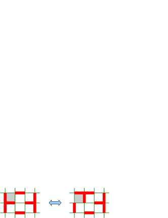
Figure 1: (Color online) “Star” configurations of dimers on the square lattice and their possible hopping.

IV.2 QDM at $\mu\to\infty$

Quite remarkably, another reduction to a dimer model is implemented in the opposite limit $\mu\to\infty$ (at finite values of $U$ and $W$). In this limit, potential energy vanishes for all plaquettes without dimers and for plaquettes with one dimer, is equal to $U$ for plaquettes with two dimers and is infinite for plaquettes with three or more dimers. This splits the Hilbert space of the system into sectors with different number of dimers, because all processes changing this number are prohibited. In particular, the sector with the smallest possible number of dimers corresponds to the standard situation when any site belongs to only one dimer. Within this sector the Hamiltonian (9) is completely equivalent to the RK Hamiltonian (1) with $v=U$ and $t=W$.

Other sectors involve configurations with overlapping dimers (see Fig. 1) that we call below “stars.” Since each star adds one extra dimer, these sectors can be labeled by the total number of stars in the system. We can therefore refer to the model obtained in the $\mu\to\infty$ limit as a “star-dimer model.” In terms of the height representation for dimer coverings of the square lattice, Levitov90 ; Henley97 each star corresponds to a screw dislocation, whose sign depends on to which of the two sublattices this star belongs.

A relevant question in such a situation is whether the “starless” sector is indeed the lowest-energy sector of the model. At $U=W$, one can show that, while a single-star configuration has the same zero energy as the RK ground state, starting from two stars, the ground-state energy becomes positive. This is a consequence of a contact repulsive interaction between stars: when stars are close to each other, some flips on plaquettes with two dimers would produce plaquettes with three dimers and therefore are prohibited. Accordingly, the kinetic energy cannot fully compensate the potential one. Since on a bipartite lattice stars are “charged” (with each star occupying three sites from one sublattice and only one from the other), they can appear in a finite system only in pairs, and therefore the one-star sector can be disregarded. We can then summarize our conclusion that, at $U=W$, the starless sector has the lowest ground-state energy.

Is is also possible to prove that the starless sector gives the lowest-energy state at $U>W$. In this case, the staggered state, in which each plaquette contains only one dimer and therefore no fluctuations are possible, realizes the ground state of the model [the same nonflippable state is known RK to be the ground state of the RK model (1) at $v>t$]. Indeed, since the full Hamiltonian may be represented as

$$H(U,W)=H(W,W)+H(U-W,0)\,,$$ (10)

and the nonflippable state is a ground state of both $H(W,W)$ and $H(U-W,0)$ (at $U>W$), it must also be a ground state of $H(U,W)$ (without regard to a sector).

For $U<W$, the situation is more complicated: the sectors with stars may, in principle, have lower energy than the ground state of the RK model. While the latter is known to be crystal-ordered (with the plaquette or columnar type of order LChR ; Sachdev89 ; Syl06 ; RPM ), it may be possible that in some interval of $Y$ stars are energetically favorable (which would possibly modify or destroy the crystal order). A simple perturbative study of stars doped into the liquid at the RK point $Y=1$ suggests that stars are not energetically favorable in the star-dimer model near the RK point. However, for a rigorous justification of the absence of stars, a more careful (possibly numerical) study is necessary, which takes into account the presence of a crystalline order. We do not address this issue in the present work, but leave it for future studies.

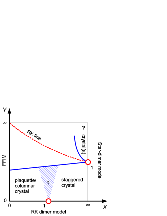
Figure 2: (Color-online) A schematic representation of the phase diagram of the two-parameter model (9) on the square lattice, in the coordinates (11).

IV.3 Phase diagram

Constructing a full phase diagram of the model (9) is a challenging problem. The model depends on two dimensionless parameters $\mu$ and $U/W$, and already the boundary of this parameter domain contains several interesting models, including those discussed above (FFIM, RK dimer model, and the star-dimer model).

For a better visualization of the discussed limiting cases, we choose the coordinates for the phase diagram as follows:

$$X=\frac{U}{W}\sinh^{2}(2\mu)\,,~{}~{}~{}Y=\frac{W}{U}\coth(2\mu)\,.$$ (11)

Our proposal for the phase diagram in these coordinates is schematically shown in Fig. 2. The vertical axis $X=0$ corresponds to the FFIM with $\Gamma/J=Y$, and the horizontal axis $Y=0$ to the RK model with $v/t=X$. The $X\to\infty$ limit corresponds to the star-dimer model whose starless sector is given by the RK dimer model with $t/v=Y$. At least for $0\leq Y\leq 1$, the true ground state of the model (9) belongs to this sector.

In terms of the original variables $U$, $W$ and $\mu$, the point $X=\infty$, $Y=0$ corresponds to $W=0$ and, naturally, can be achieved at any $\mu$ (which in terms of Fig. 2 corresponds to approaching this point from any direction within the square). For any $\mu$ the potential energy of the considered model is minimized in the staggered states in which all plaquettes contain exactly one dimer, $n_{i}\equiv 1$. Comparison of this energy with the potential energy of the states with small numbers of plaquettes with $n_{i}\neq 1$ suggests that for $W/U\ll\max(1,\mu)$ the quantum fluctuations on the background of a staggered state are weak and cannot destroy it. In conjunction with knowing that the staggered states are the ground states of the model both at $X\geq 1$, $Y=0$ and at $X=\infty$, $Y\leq 1$, this allows one to expect that in a finite region of the phase diagram the ground state has the same type of ordering.

The “RK line” $U=W$ at which the ground state is given by Eq. (3) corresponds to $Y=1+1/\sqrt{X}$. Since at this line the system is in the RVB state with a finite correlation radius, one expects that the RVB state occupies a finite region on the phase diagram (in the vicinity of the RK line). This region has to extend to the upper part of the axis $X=0$, which corresponds to the translationally invariant disordered phase of the FFIM.

Below a certain critical value of $Y$, the FFIM is in an ordered phase with a broken translational invariance. At $\Gamma/J=0$ (which corresponds to the point $X=Y=0$ in the lower left corner of our phase diagram), this phase is connected to the crystal phase of the RK dimer model at small values of $v/t$.

Furthermore, one can argue that the crystalline orders present in the RK dimer model (i.e., at $Y=0$) extend to a finite region of the phase diagram at $Y>0$. Indeed, at small $Y$, the potential energy of a star is large, $E_{\rm st}\approx 4U\mu\approx 2t/Y$. Therefore, at $Y\ll 1$, star configurations appear only as virtual pairs and may be taken into account as perturbative corrections within the quantum dimer model. In particular, the lowest order processes lead to the renormalization of $v$ and to the appearance of an additional kinetic term related to a cyclic flip of three dimers belonging to two neighboring plaquettes. The amplitude of these corrections is proportional to $1/Y$, and therefore their presence cannot destroy the crystalline phases of the RK model in some region above the $Y=0$ line.

As revealed by numerical studies of the RK dimer model, LChR ; Syl06 ; RPM at $0<v/t<1$ its phase diagram contains at least two different crystal phases: the plaquette and columnar ones. Therefore, the lower left part of our phase diagram must also contain two or more crystal phases.

It follows from the analysis of Ref. FHMOS, that the transition between the rightmost of these phases and the staggered crystal occupying the lower right part of the phase diagram may occur along one of the two scenarios: either as a first-order transition line terminating at the RK point ($X=1$, $Y=0$) or as a devil’s staircase (complete or incomplete) of intermediate commensurate phases. In either case, we do not expect any RVB region in the vicinity of the RK point.

Yet another crystal region is expected to exist at the vertical axis $X=\infty$ above the RK point $Y=1$. As mentioned in the previous subsection, a simple variational analysis of stars doped into the RK state indicates that they should be energetically unfavorable just above the $Y=1$ point. Therefore a plaquette crystal is expected in the dimer-star model adjacent to this point.

A deviation from the $X=\infty$ axis leads to the mixing between the different sectors of the star-dimer model. The difference from the region just above the line $Y=0$ is that, in the vicinity of the $X=\infty$ axis, the proper energy of a star is not high. However, at $X\gg 1$, the amplitude of the formation of a pair of stars is low. In addition to that, the presence of the crystalline order in the starless sector induces a linear in distance attraction between the stars. It appears because, in terms of the height representation, stars correspond to screw dislocations. The combination of these factors leads to the confinement of stars and does not allow them to destroy a crystalline order in some vicinity of the $X=\infty$ axis (more precisely, of its part where the star-dimer model is in the crystal phase). On the other hand, when deviation from the $X=\infty$ axis takes place at $Y=1$, the confining interaction between the stars induced by the crystalline order is absent and one immediately gets into the RVB phase.

Further interesting phases may be possible in the upper right corner of the phase diagram, with stars playing a role in the energetic balance. In the present work, we do not explore this region of the phase diagram, but leave this for future studies.

V Triangular QDM / Honeycomb FFIM lattice

In this section, we consider the same model (9) in the case of the triangular QDM lattice, which corresponds to the honeycomb FFIM lattice. As on the square lattice, the FFIM limit is achieved in the limit $\mu\rightarrow 0$ taken at $U\mu/W={\rm const}$, as is explained in more detail in Sec. III.2. The dimer limit is, however, rather different from the square-lattice case. The reason for this difference is that, on the triangular lattice, the constraint of nonoverlapping dimers prohibits direct flips induced by operators $\sigma^{z}_{j}$, and the dynamics of dimers has to be mediated by virtual flips via intermediate non-dimer states. Since the magnitude of the gap to the nondimer states in the Hamiltonian (9) is of the order of $U\sinh\mu$, the dimer model can be expected to be realized when $W/(U\sinh\mu)\to 0$. In this limit, the only terms which survive in the effective Hamiltonian for the dimer model come from the second order of the perturbation theory.

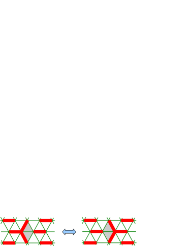
Figure 3: (Color online) “Star” configurations of dimers on the triangular lattice and their possible hopping.

Similarly to the “star-dimer” limit on the square lattice, the peculiarity of the limit $W/(U\sinh\mu)\to 0$ on the triangular QDM / honeycomb FFIM lattice is that the potential term in Hamiltonian (9) does not impose the rigorous dimer constraint but prohibits only having more than one dimer on every triangular plaquette. In addition to the usual (non-overlapping) dimer coverings this also permits the star-like overlaps of three dimers forming angles $120^{\circ}$ with respect to each other (see Fig. 3). As a consequence, the effective model obtained in the considered limit contains not only the dimer sector, but also the sectors with such three-dimer stars. As in the star-dimer model on a square lattice these sectors differ by the number of dimers: each star adds one extra dimer.

V.1 Rokhsar–Kivelson limit

We first discuss the RK-point limit, which is realized when $W/(U\sinh\mu)\to 0$ while $\mu\to\infty$. In this limit, the only terms which survive in the effective Hamiltonian for the dimer model are related to virtual flips on triangular plaquettes with one dimer. Analogous flips on plaquettes without dimers can be neglected since they lead to intermediate states with three dimers per plaquette (which for $\mu\to\infty$ are infinitely higher in energy than the intermediate states with two dimers per plaquette). Then, in the dimer sector (without stars), we arrive at the RK Hamiltonian with $v=t=W^{2}/(2U\sinh\mu)$.

In the case of sectors with stars, however, second-order perturbation theory shows an imbalance between the potential and the kinetic terms. Namely, for each star, there is a positive potential contribution of the order $W^{2}/(U\sinh\mu)$, which is not compensated by a kinetic term. We then conclude that configurations with stars are separated by a finite gap from the RK dimer sector, the magnitude of the gap being of the order of the coupling constant of the RK model.

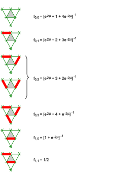
Figure 4: (Color online) The coefficients $f_{n,\bar{n}}$ entering Eq. (12) for different configurations of dimers on the plaquette ${\cal P}_{i}$ (shaded triangle in the middle) and the three neighboring plaquettes.

V.2 QDM at finite $\mu$

A more general QDM is obtained when the limit $W/(U\sinh\mu)\to 0$ is taken at a finite value of $\mu$. In this case, the effective kinetic term is also of the RK type with $t=W^{2}/(2U\sinh\mu)$. The effective potential energy becomes, however, more complicated, because at $\mu<\infty$ the virtual flips on triangular plaquettes without dimers also have to be taken into account.

In any configuration with only nonoverlapping dimers, a virtual flip on the plaquette ${\cal P}_{i}$ produces a gain of the potential energy

$$E_{i}=-\frac{W^{2}}{2U\sinh\mu}\,f_{n_{i},\bar{n}_{i}}(\mu)\,,$$ (12)

where factors $f_{n_{i},\bar{n}_{i}}(\mu)$ depend on $n_{i}$, the number of dimers on ${\cal P}_{i}$, and $\bar{n}_{i}$, the total number of dimers belonging to the three neighboring plaquettes of ${\cal P}_{i}$ but not belonging to ${\cal P}_{i}$. Fig. 4 shows the values of these factors for all possible configurations of dimers on ${\cal P}_{i}$ and the three neighboring plaquettes. It is not hard to notice that $1/f_{n,\bar{n}}(\mu)$ depends linearly on both $n$ and $\bar{n}$, which allows us to replace the six formulas shown in Fig. 4 by a single expression,

$$f_{n,\bar{n}}(\mu)=[(1-n)e^{2\mu}+1+\bar{n}+(4-3n-\bar{n})e^{-2\mu}]^{-1}.$$ (13)

The potential energy given by the sum $\sum_{i}E_{i}$ may be alternatively described in terms of local interactions between dimers. In this description, in addition to $v$, the energy of the interaction of nearest-neighbor dimers [see Fig. 5(a)], one needs to introduce two other coupling constants describing the interaction of next-nearest-neighbor dimers. We denote the pairwise interaction of such dimers as $v_{2}$ [see Figs. 5(b) and 5(c)], whereas $K$ denotes an additional three-body interaction in a loop of next-nearest-neighbor dimers [Fig. 5(d)]. These definitions imply that the dimer configurations shown in Figs. 5(b) and 5(c) are ascribed the energy $v_{2}$, whereas the configuration of Fig. 5(d) is ascribed the energy $3v_{2}+K$. After straightforward algebra one obtains

$$v/t = \tanh\mu-2(f_{0,0}-f_{0,1})\,,$$ (14a)

$$v_{2}/t = -(f_{0,0}-2f_{0,1}+f_{0,2})\,,$$ (14b)

$$K/t = f_{0,0}-3f_{0,1}+3f_{0,2}-f_{0,3}\,,$$ (14c)

where the argument of the functions $f_{0,\bar{n}}(\mu)$ is omitted.

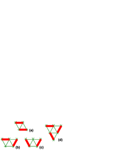
Figure 5: (Color online) The potential energy given by the sum $\sum_{i}E_{i}$ may be reproduced by attributing energy $v$ to each pair of neighboring dimers (a), energy $v_{2}$ to each pair of next-nearest-neighbor dimers [(b) and (c)] and an additional energy $K$ to each three-dimer loop (d).

In Eq. (14a), the relative magnitude of the second (negative) term never exceeds $0.12$ and vanishes in the limit $\mu\to\infty$. The functional dependence of $v/t$ on $\mu$ is monotonic, with $v/t$ ranging from $0$ to $1$ as $\mu$ ranges from zero to infinity. Since the magnitudes of coupling constants $v_{2}$ and $K$ are always numerically small ($-0.0042<v_{2}/t<0$ and $0<K/t<0.0012$, for any $\mu$ between zero and infinity, see Fig. 6), the resulting QDM can be understood as a small deformation of the RK Hamiltonian with $v/t$ given by Eq. (14a). At $\mu\to 0$ and at $\mu\to\infty$ both $v_{2}$ and $K$ tend to zero and one recovers the RK model (1) with $v=0$ and $v=t$ respectively.

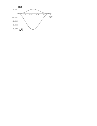
Figure 6: $v_{2}$ and $K$ as functions of $v$.

As for the star configurations, we have not analyzed their energies between the two limits $\mu\to 0$ and $\mu\to\infty$. Since at $\mu\to\infty$ their energy is positive and at $\mu\to 0$ it becomes infinite, we conjecture that it remains positive also at intermediate values of $\mu$, so that the dimer sector is always the lowest-energy sector of the model. However, a rigorous verification of this property is probably possible only numerically.

V.3 Phase diagram

Based on the above consideration of the two limits, it is convenient to plot the phase diagram of the model (9) on the triangular lattice in the coordinates $\mu$ and

$$y=\frac{W}{2U\sinh\mu}\,,$$ (15)

see Fig. 7. The vertical axis ($\mu=0$) corresponds to the FFIM with $\Gamma/J=y$, and the horizontal axis ($y=0$) to the QDM. This QDM differs slightly from the RK model with $v/t\approx\tanh\mu$ due to the presence of the additional interactions between the next-to-nearest dimers described by the coupling constants $v_{2}$ and $K$ [see Eqs. (14b) and (14c)]. However these interactions are always very weak and vanish when $\mu\to 0$ and $\mu\to\infty$ when the model (9) becomes (in its dimer sector) exactly equivalent to the RK model (1) with $v=0$ and $v=t$ respectively.

At $v/t=0.83(2)$ the RK dimer model on the triangular lattice experiences a phase transition from the RVB to the crystal phase. Ralko A possible structure of this crystal phase has been discussed not only in the context of the RK dimer model but also in the context of the FFIM on the honeycomb lattice. The most likely crystal configuration has a 12-site unit cell in the QDM formulation MS01prb ; Ralko corresponding to a 24-site unit cell in the FFIM formulation. Coletta We expect that, similarly to the RK model, our limiting dimer model obtained in the limit $y\to 0$ behaves in the same way. It seems to us unlikely that the very weak additional interactions by which this model differs from the RK model can lead to the formation of other (more complicated) crystals. Since the crystal phase with the same structure exists also in the FFIM at small enough values of $y$, it can be expected to occupy a finite region in the lower left corner of the phase diagram (see Fig. 7).

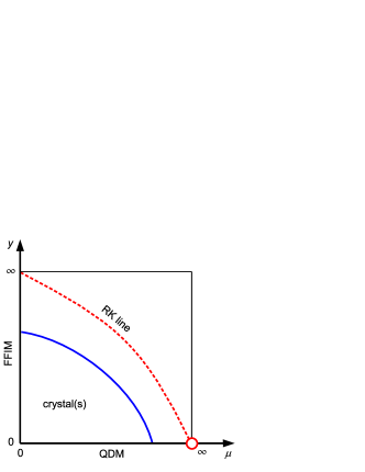
Figure 7: (Color online) A schematic representation of the phase diagram of the two-parameter model (9) on the triangular lattice in the coordinates $\mu$ and $y=W/(2U\sinh\mu)$.

The RVB phase of the RK model spans the interval between $v/t\approx 0.83$ and $v/t=1$, which corresponds to $\mu>1.22$, according to Eq. (14a). In this region, the next-nearest-neighbor interactions are very weak. In particular, at the transition point $-v_{2}/t\sim 10^{-3}$ and $K/t\sim 10^{-4}$ with a further rapid decay at $v/t\to 1$, the asymptotic behavior being $v_{2}/t\approx-(1/4)(1-v/t)^{3}$ and $K/t\approx({3}/{8})(1-v/t)^{4}$. This suggests that the presence of the additional interactions cannot induce a noticeable shift of the position of phase transition in comparison with the RK model or have any influence on the properties of the RVB phase.

The exactly solvable line is given in our coordinates by $y=1/(2\sinh\mu)$. It follows from the exact solution of the classical antiferromagnetic Ising model on the triangular lattice Stephenson that the ground state (3) has a finite correlation length everywhere on this line, and therefore we expect that this line lies fully outside the crystal phase in our phase diagram. Note that the staggered (non-flippable) phase of the RK dimer model, which appears at $v/t>1$, is not present in our phase diagram, since this region of parameters cannot be reached within our model. We can only span the region between $v/t=0$ and $v/t=1$, with additional interactions of next-nearest-neighbor dimers which are always too weak to stabilize the staggered phase.

VI Conclusion

In this work, we have constructed a model interpolating between a quantum dimer model and a fully frustrated Ising model in a transverse field and studied its phase diagram for square and triangular (in terms of the dimer representation) lattices. This interpolating model exhibits an RVB phase, including a special “RK line” with an exactly solvable ground state. This RK-type ground state generalizes the construction at the RK point of the quantum dimer model, with its equal-time correlations given by the classical fully frustrated Ising model (without a field) at a finite temperature.

While the RK dimer model is a well-known “prototype model” of the RVB phase, our construction may be considered as its generalization including “star” configurations. It can be useful for studying the role of spin and charge degrees of freedom in RVB states.

Indeed, a qualitative description of the RVB state in a spin system contains elementary spin excitations (spinons) and vortexlike excitations (visons). In application to high-temperature superconductivity, it has been also suggested that doping RVB liquids gives rise to charge excitations (vacancies or holons).Read-Chakraborty ; KRS ; Senthil-Fisher At the same time, the RVB state in the pure dimer model only contains visons as elementary excitations, with spinons and holons prohibited by the close-packing dimer constraint. From this point of view, the model constructed in the present work may serve as a prototype model of an RVB state including both visons and holons (since star configurations carry extra charge).

Finally, we would like to note a certain similarity between the appearance of RVB states on the square lattice close to the critical RK points in the model of the present work (the point $X=\infty$, $Y=1$ in the phase diagram in Fig. 2) and in that of Ref. Strubi, . In both situations, the initial RK state is deformed into an RVB state by introducing a small concentration of charged objects (stars in the present work and diagonal dimers in Ref. Strubi, ). One may note that, in both cases, the charged defects cost initially zero energy and the deformation is achieved by tuning the amplitude of their creation and annihilation. On the other hand, if one starts with charged defects of infinite energy (which is the case at the point $X=1$, $Y=0$ in the phase diagram in Fig. 2), then the critical dimer state on the bipartite square lattice cannot be continuously deformed into an RVB state (see also the discussion in Refs. FHMOS, and Vishwanath, ).

There is also an interesting possibility that new phases may become possible in our interpolating model, e.g., superfluid or supersolid ones. We did not explore those possibilities in our analysis, but leave this question for future studies.

- (1) C. Lhuillier and G. Misguich, in High Magnetic Fields, Lecture Notes in Physics, Vol. 595, edited by C. Berthier, L. P. Lévy, and G. Martinez (Springer, Berlin, 2002); C. Lhuillier, arXiv:cond-mat/0502464 and references therein.
- (2) P. Fazekas and P. W. Anderson, Philos. Mag. 30, 423 (1974).
- (3) P. W. Anderson, Science 235, 1196 (1987).
- (4) L. Balents, M. P. A. Fisher, and S. M. Girvin, Phys. Rev. B 65, 224412 (2002).
- (5) T. Senthil and O. Motrunich, Phys. Rev. B 66, 205104 (2002); O. I. Motrunich and T. Senthil, Phys. Rev. Lett. 89, 277004 (2002).
- (6) L. B. Ioffe and M. V. Feigel’man, Phys. Rev. B 66, 224503 (2002); B. Douçot, M. V. Feigel’man and L. B. Ioffe, Phys. Rev. Lett. 90, 107003 (2003).
- (7) A. Seidel, Phys. Rev. B 80, 165131 (2009).
- (8) R. Moessner and S. L. Sondhi, Phys. Rev. Lett. 86, 1881 (2001).
- (9) G. Misguich, D. Serban, V. Pasquier, Phys. Rev. Lett. 89, 137202 (2002).
- (10) J. S. Helton et al, Phys. Rev. Lett. 98, 107204 (2007); P. Mendels et al, Phys. Rev. Lett. 98, 077204 (2007); O. Ofer et al, arXiv:cond-mat/0610540.
- (11) C. Waldtmann et al, Eur. Phys. J. B 2, 501 (1998).
- (12) D. Schwandt, M. Mambrini, and D. Poilblanc, Phys. Rev. B 81, 214413 (2010).
- (13) R. Moessner, S. L. Sondhi, and P. Chandra, Phys. Rev. Lett. 84, 4457 (2000).
- (14) R. Moessner and S. L. Sondhi, Phys. Rev. B 63, 224401 (2001).
- (15) S. Sachdev, Phys. Rev. B 40, 5204 (1989).
- (16) O. F. Syljuåsen, Phys. Rev. B 73, 245105 (2006).
- (17) N. Read and B. Chakraborty, Phys. Rev. B 40, 7133 (1989).
- (18) S. A. Kivelson, D. S. Rokhsar, and J. P. Sethna, Phys. Rev. B 35, 8865 (1987).
- (19) T. Senthil and M. P. A. Fisher, Phys. Rev. B 62, 7850 (2000); ibid. 63, 134521 (2001).
- (20) G. Misguich and F. Mila, Phys. Rev. B 77, 134421 (2008).
- (21) D. S. Rokhsar and S. A. Kivelson, Phys. Rev. Lett. 61, 2376 (1988).
- (22) P. Fendley, R. Moessner, and S. L. Sondhi, Phys. Rev. B 66, 214513 (2002).
- (23) A. Ioselevich, D. A. Ivanov, and M. V. Feigel’man, Phys. Rev. B 66, 174405 (2002).
- (24) D. A. Ivanov, Phys. Rev. B 70, 094430 (2004).
- (25) A. Ralko, M. Ferrero, F. Becca, D. Ivanov, and F. Mila, Phys. Rev. B 71, 224109 (2005); ibid. 74, 134301 (2006); ibid. 76, 140404(R) (2007).
- (26) P. W. Leung, K. C. Chiu, and K. J. Runge, Phys. Rev. B 54, 12938 (1996).
- (27) A. Ralko, D. Poilblanc and R. Moessner, Phys. Rev. Lett. 100, 037201 (2008).
- (28) E. Fradkin, D. A. Huse, R. Moessner, V. Oganesyan, and S. L. Sondhi, Phys. Rev. B 69, 224415 (2004).
- (29) R. Moessner and K. S. Raman, in Introduction to Frustrated Magnetism, edited by C. Lacroix, P. Mendels and F. Mila (Springer Verlag, Heidelberg, 2011); arXiv:0809.3051.
- (30) R. Moessner and S. L. Sondhi, Phys. Rev. B 68, 054405 (2003).
- (31) C. L. Henley, J. Phys.: Condens. Matter 16, S891 (2004).
- (32) R. Liebmann, Statistical Mechanics of Periodic Frustrated Ising Systems (Springer, Berlin, 1986).
- (33) C. L. Henley, J. Stat. Phys. 89, 483 (1997).
- (34) A. M. Läuchli, S. Capponi, and F. F. Assaad, J. Stat. Mech. P01010 (2008).
- (35) L. S. Levitov, Phys. Rev. Lett. 64, 92 (1990).
- (36) T. Coletta, J.-D. Picon, S. E. Korshunov, and F. Mila, Phys. Rev. B 83, 054402 (2011).
- (37) J. Stephenson, J. Math. Phys. 11, 413 (1970).
- (38) G. Strübi and D. A. Ivanov, EPL 94, 57003 (2011).
- (39) A. Vishwanath, L. Balents and T. Senthil, Phys. Rev. B 69, 224416 (2004).