Effects of rotation on stellar p-mode frequencies

Abstract

Effects of stellar rotation on adiabatic oscillation frequencies of pressure modes are discussed. Methods to evaluate them are briefly exposed and some of their main results are presented.

1 Introduction

Many pulsating stars oscillate with pressure (or p-) normal modes for which pressure gradient is the main restoring force. A nonrotating star keeps its spherical symmetry; consequently, frequencies of its free vibrational modes are $2\ell+1$ degenerated when using a description by means of spherical harmonics, $Y_{\ell}^{m}$ ($\ell$ the degree, $m$ the azimuthal indice) for the angular dependence of the variations. However, stars are rotating and their rotation affects their oscillation frequencies. This is an advantage since rotation breaks the spherical symmetry of the star; as a consequence, the $2\ell+1$ degeneracy is lifted and gives access to information about the internal rotation. The information is relatively easy to extract if the star rotates slowly provided observations are of high quality enough that they enable to achieve the necessary high accuracy of frequency measurements. On the other hand, when the star is rotating fast, one must properly take into account the consequences of the spheroidal shape of the star on the oscillation frequencies before extracting seismological information on the internal structure or the rotation profile of the star. Three methods have been used to investigate the effect of rotation on oscillation frequencies of stellar pressure modes: a variational principle, perturbation techniques and direct numerical integration of a two dimensional eigenvalue system. We briefly describe the 3 methods and their main results. All these methods assume the knowledge of the structure of the distorted star, which is obtained either by perturbation or by 2D calculations. This is also sketched when appropriate.

This lecture is priorily adressed to PhD students who possess some basic background in stellar seismology but wish to learn with some details how to handle the impacts of the rotation on the oscillation frequencies of a star. The present lecture cannot be exhaustive neither in the credit to authors nor to the numerous effects of rotation on stellar pulsation. Indeed, due to the importance of stellar rotation in a more general astrophysical context, a tremendous amount of work has been performed on stellar rotation and its interaction with stellar oscillations since the 1940-1950s. For more details, we refer the reader to standard text books such as Ledoux & Walraven (1958); Cox (1980); Unno et al (1989) and to litterature on the subject: Gough,Thompson (1991), Gough (1993), Christensen-Dalsgaard (2003, CD03) and references therein.

The organization of this contribution is as follows: as a start, some definitions and orders of magnitude are given in Sect.2. Sect.3 introduces the basic background in deriving the wave equation and eigenvalue problem modelling the adiabatic pulsations of a rotating star. Sect.4 discusses the existence and consequence of a variational principle for rotating stars. Sect.5 and 6 respectively concern calculation of the oscillation frequencies of respectively slowly and modetately rotating stars by means of perturbation methods. Sect.7 then turns to fast rotating stars and the computation of their oscillation frequencies with nonperturbative techniques. Some comparisons of the results of perturbative and nonpertubative methods and comments on the range of validity of the first ones are given in the case of polytropic models. Sect.8 briefly discusses observations of real stars and forward inferences on stellar internal rotation sofar derived. Sect.9 turns to inverse methods specifically applied to obtain the internal rotation profile. Finally results of inversions for the rotation profiles of some stars are presented in Sect.9. To keep up with the allowed number of pages, the choice has been to show almost no figures and rather to refer in the text to plots in the litterature. Some illustrations of the consequences of rotation on pulsations of stars can also be found in Goupil et al. (2006).

2 Definitions and orders of magnitude

We will denote $\omega^{(0)}_{n,\ell}$ the pulsation of an oscillation mode with radial order $n$ and degree $\ell$ for a nonrotating star and $\nu^{(0)}_{n,\ell}=\omega^{(0)}_{n,\ell}/2\pi$ the associated frequency in $Hz$. For a symmetric star of radius $R$ and mass $M$ and for any given eigenfrequency $\omega$, we define the dimensionless frequency, $\sigma$:

$$\sigma={\omega\over(GM/R^{3})^{1/2}}$$ (1)

Consider now a star which rotates with a rotational period $P_{rot}$. We denote $\Omega=2\pi/P_{rot}$, its angular rotational velocity. One also defines the equatorial velocity $v_{eq}=R_{eq}\Omega$ where $R_{eq}$ is the equatorial stellar radius, this is the velocity of the fluid at the equatorial level generated by rotation. One also uses the projected velocity $v\sin i$ where $i$ is the angle between the line of sight and the rotation axis.

2.1 Why are the oscillation frequencies of a rotating star modified compared to those a nonrotating star ?

(i) A first effect is easy to understand as it is purely geometric. Let consider a uniformaly rotating star which oscillates with a pulsation frequency $\omega^{(0)}_{n,\ell}$ in the rotating frame. In an inertial frame, an observer will see oscillations with frequencies given by $\omega_{n,\ell,m}=\omega^{(0)}_{n,\ell}+m\Omega$ with $m\in[-\ell,\ell]$ with progade ($m>0$) et retrograde ($m<0$) modes. Each $(n,\ell)$ mode appears in a power spectrum as a frequency multiplet split by rotation composed of $2\ell+1$ components.

(ii) At the same level (i.e. linear in the rotational angular velocity $O(\Omega)$), one must also take into account intrinsic effects of rotation in the rotating frame related to the Coriolis force which directly acts on the oscillating fluid velocity, deflecting the wave. Ledoux (1951) has shown that the Coriolis acceleration modifies the pulsation such that in the observer frame, it becomes:

$$\omega_{n,\ell,m}=\omega^{(0)}_{n,\ell}+m\Omega(1-C_{n,\ell})+O(\Omega^{2})$$ (2)

where $C_{n,\ell}$ is the Ledoux constant. The rotation rate then is simply given by

$$\Omega=(\omega_{n,\ell,m}-\omega^{(0)}_{n,\ell})/(m(1-C_{n,\ell}))$$ (3)

where the Ledoux constant is assumed to be known from a nonrotating stellar model. However, the rotation of a star is not necessarily uniform: it can vary with latitude and depth; this again results in modifications of the frequencies. Actually these modifications are those one really wishes to identify. Indeed current open issues are: what are the regions inside the star where the rotation is uniform and where it is not? how strong are rotational gradients? what are the mechanisms which make the region uniform or in contrary generate differential rotation? how to model them ot test the validity of their modelling?

The magnitude of the above effects are proportional to $\Omega$. For a slowly rotating star indeed, effects of the centrifugal force, proportional to $\Omega^{2}$, on oscillation frequencies are small and one usually ignores them. The rotational splitting of a mode with given $(n,\ell)$ then is defined as:

$$\delta\omega_{n,\ell}={\omega_{n,\ell,m}-\omega_{n,\ell,0}\over m}$$ (4)

where $\omega_{n,\ell,0}$ can reasonably be identified with $\omega^{(0)}_{n,\ell}$ for a slow rotating star.

(iii) For stars rotating faster, one must take into account the various effects due to the distorsion of the star by the centrifugal force:

‘mechanical’ impact: the centrifugal force affects the wave propagation by deforming the resonant cavity where they propagate. Pioneer studies were due to Ledoux (1945) and Cowling, Newing (1949). Ledoux (1945) studied radial oscillations of a uniformaly rotating star by means of a variational principle and assuming uniform dilation and compression motions. He obtained the squared frequency of the fundamental radial mode under the influence of the centrifugal force as

$$\omega^{2}=-(3\Gamma_{1}-4){E_{g}\over I_{0}}+(5-3\Gamma_{1})2T$$

where $I_{0},\Gamma_{1},E_{g},T$ respectively denote the moment of inertia, the adiabatic exponent (assumed constant throughout the star), gravitational potential and rotational kinetic energies. For a homogeneous spheroid in uniform rotation (Simon, 1969), $E_{p}/I_{0}\sim 4\pi G\rho$ decreases whereas $T={\cal M}/I_{0}\sim\Omega^{2}/3$ increases (${\cal M}$ is the total angular momentum) when $\Omega$ increases. Cowling, Newing (1949) extended the study to nonradial oscillations of a rotating configuration and obtained numerical results for radial oscillations of a polytrope.

In order to obtain the rotational profile, one defines the generalized rotational splitting of a mode with given $(n,\ell)$ as:

$$S_{m}={\omega_{m}-\omega_{-m}\over 2m}$$ (5)

This 2nd definition eliminates second order perturbation effects (cf Sect.6.2) that-is eliminates the mechanical effects of the nonspherically symmetric distorsion of the star on the oscillation frequencies.

‘thermal’ impact: Works by Von Zeipel (1924ab), Eddington (1929), Vogt (1929), Sweet (1950) showed that the non spherical shape of a rotating star causes a departure from thermal equilibrium which generates large scale meridional currents. As already emphasized by Ledoux (1945), this meridional circulation can influence the pulsations. Indeed it generates a differential rotation which causes hydrodynamical instabilities. The net effect results in transport of chemical elements and angular momentum in radiative regions and modifications of the thermodynamical state of the star. All these processes influence the star evolution and structure (Tassoul (1978), Zahn (1992); see also Meynet , Maeder, (2000); Mestel (2003); Zahn (2003) for reviews), in particular the adiabatic sound speed and the rotation profile, the two main quantities accessible with seismology. Hence it is important to note that even for a star which is assumed to be in near spherical symmetry and with a given rotation profile at the time of observation, there exists a nonzero difference between the zeroth order eigenfrequencies of a rotating model which has been evolved taking into account the effect of rotation and that of an ’equivalent’ model at the same age evolved without rotation in which effect of rotation law is imposed afterward or which has been evolved with rotation included only through the effective gravity. For a slow rotating star however, this difference can often be neglected.

2.2 How to determine the frequency changes due to rotation?

The methods which must be used in order to determine precisely how and how much the oscillation frequencies are affected by rotation can be divided into 2 groups (apart from the variational technique): the perturbative methods on one hand and the direct numerical approaches or non perturbative methods on the other hand. The choice will depend whether the star is a rather slow or rather fast rotator. This classification can be loosely made according to values of dimensionless parameters. The ratio of the time scales related to Coriolis force and pulsation is roughly given:

$$\mu={P\over P_{rot}}={\Omega\over\omega}$$ (6)

Another important parameter is the ratio of rotational kinetic energy to the gravitational one. As an order of magnitude, it can be evaluated as

$$\epsilon_{eq}={\Omega^{2}R_{eq}^{2}\over GM/R_{eq}}={\Omega^{2}\over(GM/R_{eq}^{3})}=\mu^{2}~{}\sigma^{2}$$ (7)

where $M$ is the mass of the star ; $R_{eq}$ its radius at the equator; $G$ is the gravitational constant. One also uses the flatness, $f$, as defined by $f=1-{R_{pol}/R_{eq}}$ where $R_{pol}$ is the radius at the pole.

In the following sections, we will then distinguish fast, moderate and slow rotators with respect to the pulsations of the stars according to these parameters. Stars for which these parameters obey ($\mu,\epsilon<<1$ ),  ($\mu,\epsilon<0.3$) or ( $\mu$ or $\epsilon>0.3$) are classified respectively as slow, moderate or fast rotators. For slow rotators, a first order perturbation is enough; for a moderate rotator, a perturbation method can still be valid provided higher order contributions are included. Studying oscillations of fast rotators requires the use of 2D equilibrium models as well as solving a 2D eigenvalue system. However one must keep in mind that the above classification depends on the star as it depends on the frequency range of its excited modes. Perturbation methods cease indeed to be valid whenever the wavelength of the mode reaches the order of $\sim\epsilon~{}R$ where $R$ is the stellar radius that-is for p-modes with high enough frequencies.

In the solar case, $P_{rot,\odot}$ varies from $\sim 25$ days at the equator up to $P_{rot,\odot}\sim 35$ days at the poles then $\epsilon_{eq,\odot}=2.1~{}10^{-5}$ is very small. The splitting is of the order $0.456\mu$Hz with a Coriolis strength $\mu=1,4~{}10^{-4}$. With $\mu,\epsilon<<1$, the Sun is considered as a slow rotator with respect to its pulsations. However, measurements of the rotational splittings are so accurate for the Sun- one is able to determine the internal rotation velocity of the Sun as a function of radius and latitude with unprecedented spatial resolution and accuracy- that one measures second order effects in the rotational splittings which must be taken into account in order to obtain information on the solar magnetic field (Gough, Thompson, 1990 (GT90); Dziembowski & Goode, 1992 (DG92)) and to determine the gravitational quadrupole moment of the Sun with much higher accuracy (Pijpers, 1998).

For a $\delta$ Scuti-type variable star ($~{}2M_{\odot},2R_{\odot}$), observations show that $v\sin i=70-280$ km/s that-is $P_{rot}\sim 1,45$ days to $\sim 8$ hours ; this yields $\Omega=5$ to $20~{}10^{-5}$ rad/s and a rotational splitting of the order of $\nu_{rot}=8$ to $32\mu$Hz. Typical values for the dimensionless parameters then are $\epsilon=0.025-0.41$ and $\mu=0.06-0.6$ for an oscillation frequency range of $200-500\mu$Hz. Altair is an exemple of a rapidly rotating $\delta$ Scuti star with a rotation velocity between 190 and 250 km/s (Royer et al.  2002) which has been discovered to pulsate over at least 7 frequencies in the range 170-350 $\mu$Hz (Buzasi et al.  2005). With $M=1.72\pm 0.05M_{\odot}$ and $R=1.60\pm 0.12$ for its mass and radius as found in the litterature, one obtains $\epsilon\sim 0.305$ and $\mu\sim 0.09-0.2$ which definitely classes this star as a rapid rotator with respect to its pulsations.

A $\beta$ Cepheid-type variable star ($~{}9M_{\odot},5R_{\odot}$) can reach $v\sin i=300$ km/s that-is $P_{rot}<20$ hours.This yields $\Omega>8.6~{}10^{-5}$rad/s and $\nu_{rot}>14\mu$Hz. For the dimensionless parameters, one derives $\epsilon>0.26$ and for $\nu\sim 500\mu Hz$ , $\mu>2.710^{-2}$

A much more evolved star such as a Cepheid is a radially pulsating star and a slow rotator. However period ratios of radial modes can be quite significantly affected by rotation as mentionned by Pamyatnykh (2003, Fig.6) for a $\delta$ Scuti star and quantified by Suarez et al.  (2006a, 2007) for a Cepheid.

The above figures and classifications must be seen as illustrative and only a comparison between perturbative and nonperturbative approaches can give more precise delimitations between the different classes (Sect.7.3).

3 A wave equation for a rotating star

A derivation of the wave equation for a rotating star can be found in Unno et al. (1989). The basic equations for a non magnetic, self gravitating fluid are written as :

$${\partial{\bf v}\over\partial t} + {\bf v}\cdot{\bf\nabla}{\bf v}=-{1\over\rho}{\bf\nabla}p-{\bf\nabla}\psi$$ (8)

$${\partial\rho\over\partial t} + \nabla\cdot(\rho{\bf v})=0$$ (9)

$$\rho T{\partial\vec{S}\over\partial t} + \rho T({\bf v\cdot\nabla})S=\rho\epsilon-{\bf\nabla\cdot{\cal F}}$$ (10)

$$\nabla^{2}\psi = 4\pi G\rho$$ (11)

where the quantities take their usual meaning and

$$\psi(\vec{r},t)=G\int_{V}~{}{\rho(\vec{r}^{\prime},t)\over|\vec{r}-\vec{r}^{\prime}|}~{}\vec{d}^{3}r^{\prime}$$

In an inertial frame, the effect of rotation appears through the inertial term ${\bf v\cdot\nabla v}$. In the frame rotating with the star, the inertial term acts as 2 fictive forces: the Coriolis force $(-2\rho{\bf\Omega}\times{\bf v})$ which modifies the dynamics and insures the conservation of angular momentum and the centrifugal force ($-\rho{\bf\Omega}\times{\bf\Omega}\times{\bf r}$) which affects the structure of the equilibrium configuration of the star, i.e. the star is distorted and loses its spherical symmetry. The oscillations are described as a linear perturbation about an equilibrium or steady-state configuration which is assumed to be known.

3.1 Equilibrium structure for a rotating star

We assume a steady state configuration i.e. all local time derivatives vanish, the quantities describing this equilibrium are given a subscript 0, for instance the steady state velocity field is noted $\vec{v}_{0}$. The assumption of stationarity leads to:

$${1\over\rho_{0}}{\bf\nabla}p_{0}+{\bf\nabla}\psi_{0} = -{\bf v_{0}\cdot\nabla\vec{v}_{0}}$$ (12)

$${\bf\nabla\cdot}(\rho_{0}{\bf v}_{0}) = 0$$ (13)

$$\rho_{0}T_{0}({\bf v}_{0}{\bf\cdot\nabla})S_{0} = \rho_{0}\epsilon_{0}-{\bf\nabla\cdot\vec{\cal F}}_{0}$$ (14)

$$\nabla^{2}\psi_{0} = 4\pi G\rho_{0}$$ (15)

We consider an axisymmetric rotation ${\bf\Omega}$. In spherical coordinates, one has:

$$\vec{\Omega}(r,\theta)=\Omega(r,\theta)\left(\cos\theta~{}{\bf e_{r}}-\sin\theta~{}{\bf e_{\theta}}\right)$$

The large scale velocity field $\vec{v}_{0}=v_{\Omega}+\vec{U}$ is composed of the rotational velocity and the meridional circulation. We consider here that the meridional circulation has no direct effect on the dynamics of the pulsation ($U<<c_{s}$), hence one neglects it in the velocity field which therefore is only due to rotation and has the expression:

$${\bf v}_{0}({\bf r})={\bf\Omega}\times{\bf r}=\Omega(r,\theta)~{}r\sin\theta~{}{\bf e_{\phi}}$$ (16)

The steady state configuration is then given by:

$$-{1\over\rho_{0}}{\bf\nabla}p_{0}-{\bf\nabla}\psi_{0}={\bf\Omega}\times{\bf\Omega}\times{\bf r}=-r\Omega^{2}\sin\theta~{}{\bf e_{s}}$$ (17)

where ${\bf e_{s}}=\sin\theta~{}{\bf e_{r}}+\cos\theta~{}{\bf e_{\theta}}=\partial{\bf e_{\phi}}/\partial\phi$. Note that $-\vec{\Omega}\times\vec{\Omega}\times\vec{r}=r\Omega^{2}{\bf e_{r}}$ for $\theta=\pi/2$ is directed toward the $r>0$ and we recognize the centrifugal acceleration.

Particular cases: barotropy and uniform rotation

When the centrifugal force can be considered as deriving from a potential (conservative rotation law), it can be included similarly to the gravity and the equilibrium equation becomes:

$$-{1\over\rho_{0}}{\bf\nabla}p_{0}-{\bf\nabla}(\psi_{0}-|{\bf\Omega}\times{\bf r}|^{2}/2)=0$$

One sets $\psi_{eff}\equiv\psi_{0}-|{\bf\Omega}\times{\bf r}|^{2}/2$ and obtains

$${dp_{0}\over dr}=-\rho_{0}~{}g_{eff}~{}~{}~{}~{}~{}~{}~{}~{}~{}~{}~{}~{}~{}~{}{\bf\nabla\psi}_{eff}=g_{eff}$$

The star keeps it spherical symmetry. This happens for a uniform rotation or for a cylindrical rotation $d\Omega/dz=0$ in a cylindrical coordinate system (Tassoul, 1978). The Von Zeipel (1924) law states that for a barotrope and a conservative rotation law, isobars and isopycnics coincide with the level surfaces (constant potential): $\rho=\rho(\psi_{eff});T=T(\psi_{eff})$ with $\psi_{eff}=\psi+r\sin\theta\Omega$. Consequently the heat flux is proportional to local effective gravity $T_{eff}^{4}\propto g_{eff}$ and poles are hotter than the equator (gravity darkening; see Tassoul 1978 for details).

Shellular rotation $\Omega(r)$

Zahn (1992) considered that in stellar radiative regions, highly anisotropic turbulence developes: this leads to an efficient homogeneization in the horizontal plane but not in the vertical direction due to the stable stratification which inhibes vertical motions hence generating a shellular rotation. This was verified by Charbonneau (1992) by means of 2D numerical simulations. The combined effects of rotation and turbulence induce a process of advection/diffusion of angular momentum and diffusion of chemical elements. The turbulence itself can arise from a dynamical shear instability generated by the differential rotation $\Omega(\theta)$ due to the advection of angular momentum by the meridional circulation (see for a review, JP. Zahn (2005), web site of the Brasil Corot meetings, CB2; see also Talon, 2006). For rotators with no angular momentum loss, a weak meridional circulation exists only to balance transport by differential rotation induced turbulence. For rotators which lose angular momentum through a wind, the meridional circulation must adjust so as to transport momentum toward the surface. Hence effects of a complex rotationally induced 2D process can be described in a 1D framework (Zahn, (1992); Maeder, Zahn, (1998); Mathis, Zahn (2004))

2D rotation: $\Omega(r,\theta)$

Several studies have developped numerical schema in order to build more and more realistic 2D rotating stellar models. As the full problem is quite difficult, simplifying assumptions have been made depending on the purpose of the study (Clement’s series of papers from 1974 to 1998; Deupree from 1990 to 2001; see for a detailed historical review, M. Rieutord (2007), web site of the Brasil Corot meetings, CB3).

With the initial purpose of modelling the rapidly rotating, oblate Be star, Achernar, Jackson et al. (2004, 2005) neglected the evolution and dynamics of the star and focused their studies on a specified conservative rotation law. This allows them to solve a 2D partial differential equation for Poisson equation while dealing with only ordinary differential equations for the other equilibrium quantities. They were able to build stellar rotating models for a wide mass range ($2M_{\odot}$ to $9M_{\odot}$) and for equatorial velocity up to 250 km/s for the most massive ones. Roxburgh (2004) on the other hand computed 2D uniformaly rotating, barotrope zero age main sequence models again over a wide mass range and rotational velocities. The determination of the adiabatic nonradial oscillation frequencies of a rotating star only depends on the knowledge of $p_{0}(r,\theta)$, $\rho_{0}(r,\theta)$ and $\Gamma_{1}(r,\theta)$ and does not require that the thermal equilibrium be satisfied. Roxburgh (2005) takes advantage of this property to build 2-dimensional acoustic models of rapidly rotating stars with a prescribed rotation profile $\Omega(r,\theta)$. The initial density profile at a given angle $\theta_{m}$ can be taken as the density profile of a 1D stellar model (which can include effects of transport and mixing due rotation as described in the above section). Roxburgh (2005) then solves iteratively the 2D hydrostatic and Poisson equations; the adiabatic index $\Gamma_{1}$ is then obtained through the equation of state and the knowledge of the hydrogen profile (again possibly derived from the 1D spherically averaged stellar model).

In all the above studies, the $\Omega$ profile is prescribed and stellar models are built at a given evolutionary stage with no inclusion of any feedback of rotation on evolution and structure. To proceed a step further with the purpose of including effects of evolution and internal dynamics, Rieutord (2005, 2006), Espinosa Lara, Rieutord (2007) worked at building more and more realistic rotating models using spectral methods for both directions $r$ and $\theta$. Espinosa Lara, Rieutord (2007) succeeded in computing a fully radiative, baroclinic model in which the microphysics is treated in a simplified form and the star is assumed to be enclosed in a rigid sphere. Some interesting conclusions could nervertheless be drawn. For a stellar model rotating at $82\%$ of the rotational break up velocity, the baroclinic model is much less centrally condensed than a radiative polytrope. The steady state is characterized by poles hotter but rotating less rapidly than the equator. The authors found that the temperature contrast between poles and equators is less than that given by the Von Zeipel model although this might be reduced with the use of a more realistic surface boundary condition. This is also found by Lovekin & Deupree (2006) using the 2D rotating stellar code of Deupree. With increasing rotation, the equator cools down enough that a convective region seems to be able to develope. It is also found that the isothermals are more spherical that the isobars. As a consequence and in constrast with the Boussinesq case, the meridional currents circulate from equator to poles: the meridional velocity $U_{\phi}$ component decreases outward, because $T$ decreases on a isobar from pole to equator. Worth to be noting also, differential rotation in latitude seems to keep the same general form for increasing $\Omega$ between 0.01 to 0.08 of the critical rotation rate (Fig.10, Espinosa Lara, Rieutord, 2007).

3.2 Oscillations: linearization about the equilibrium

For the oscillating, rotating fluid of interest here, the velocity field in each point of the space can be split into 2 components $\vec{v}=\vec{v}_{0}+\vec{v}^{\prime}$ where $\vec{v}^{\prime}$ is the Eulerian perturbation of the velocity due to the oscillation. Similarly for any scalar quantity $f$ (such as $p,\rho,\psi$), one writes $f=f_{0}+f^{\prime}$. The quantities with a prime represent the oscillations which are modelled as linear Eulerian perturbations about the equilibrium. One inserts these decompositions into the basic equations Eq.9 and then linearizes with respect to the perturbations $\vec{v}^{\prime},\rho^{\prime}$ etc… about the equilibrium quantities. Only adiabatic oscillations are studied here, the system is then closed by using the linearized adiabatic relation:

$${\delta p\over p_{0}}=\Gamma_{1}\left({\delta\rho\over\rho_{0}}\right)~{}~{}~{}{\rm where}~{}~{}~{}~{}\Gamma_{1}\equiv\left({\partial p\over\partial\rho}\right)_{S}$$ (18)

since $\delta S=0$ ($S$ entropy) where $\delta$ denotes Lagrangian variations or in the Eulerian form:

$${p^{\prime}\over p_{0}}=\Gamma_{1}\left({\rho^{\prime}\over\rho_{0}}+{\vec{\xi}\cdot A}\right)~{}~{}{\rm where}~{}~{}{\bf A}={1\over\Gamma_{1}}{\vec{\nabla}p_{0}\over p_{0}}-{\vec{\nabla}\rho_{0}\over\rho_{0}}$$

The system of linearized equations for adiabatic nonradial oscillations of a rotating star takes the form:

$${\partial{\vec{v}^{\prime}}\over\partial t} + {\vec{v}^{\prime}\cdot\vec{\nabla}\vec{v}}_{0}+{\vec{v}}_{0}{\cdot\vec{\nabla}\vec{v}^{\prime}}=-{1\over\rho_{0}}{\vec{\nabla}}p^{\prime}+{\rho^{\prime}\over\rho_{0}^{2}}{\vec{\nabla}}p_{0}-{\vec{\nabla}}\psi^{\prime}$$ (19)

$${\partial\rho^{\prime}\over\partial t} + {\vec{\nabla}\cdot}(\rho^{\prime}{\vec{v}}_{0}+\rho_{0}{\vec{v}}^{\prime})=0$$ (20)

$${p^{\prime}\over p_{0}} = \Gamma_{1}\left({\rho^{\prime}\over\rho_{0}}-{\vec{\xi}\cdot A}\right)$$ (21)

$$\nabla^{2}\psi^{\prime} = 4\pi G\rho^{\prime}$$ (22)

The displacement is related to the Lagrangian velocity by

$${\vec{\delta}v}={D{\vec{\xi}}\over Dt}={\partial{\vec{\xi}}\over\partial t}+{\vec{v}_{0}\cdot\vec{\nabla}\vec{\xi}}$$

where ${D/Dt}$ is the Lagrangian derivative (Lebovitz, 1970). Using the linearized relation between the Lagrangian and Eulerian velocities is: ${\vec{v}^{\prime}}=\delta{\vec{v}}-({\vec{\xi}\cdot\vec{\nabla})\vec{v}_{0}}$ the Eulerian velocity perturbation ${\bf v^{\prime}}$ is related to the displacement ${\vec{\xi}}$ by:

$${\vec{v}^{\prime}}={\partial{\vec{\xi}}\over\partial t}+({\vec{v}_{0}\cdot\vec{\nabla})\vec{\xi}-(\vec{\xi}\cdot\vec{\nabla})\vec{v}_{0}}$$ (23)

3.3 Time and azimutal dependances of the oscillation

One adopts a spherical coordinate system with the polar axis coinciding with the star rotation axis. For an axisymmetric star, the system Eq.13 is separable in $\phi$ and one can then seek quite generally for a solution of the form:

$${\vec{\xi}}({\vec{r}},t)\propto{\vec{\xi}}(r,\theta,t)~{}e^{im\phi}$$

In a description based on spherical harmonics, an eigenfunction will be decomposed on the spherical harmonics with the same $m$. Because of the assumed existence of a steady state configuration, one can represent all scalar perturbations by : $f^{\prime}({\bf r},t)=f^{\prime}(r,\theta)~{}e^{i(\omega t+m\phi)}$ and for the fluid displacement vector $\vec{\xi}({\bf r},t)=\vec{\tilde{\xi}}(r,\theta)~{}e^{i(\omega t+m\phi)}$ The relation between ${\bf v^{\prime}}$ and the displacement (Eq.23) becomes:

$$\vec{v}^{\prime}=i(\omega+m\Omega)\vec{\tilde{\xi}}-(\vec{\tilde{\xi}}\cdot\vec{\nabla}\Omega)r\sin\theta\vec{e}_{\phi}$$ (24)

From now on, we drop the tilde for the displacement vector field.

3.4 The eigenvalue system

One assumes that the configuration is axisymmetric and that the motion is purely rotational i.e. one then has: $B={\bf v_{0}\cdot\nabla}=\Omega~{}{\partial/\partial\phi}$ and $Bf\equiv{\vec{v}_{0}\cdot\nabla}f=\Omega{\partial f\over\partial\phi}$ for a scalar $f$. Using Eq.13, Eq.23, Eq.24, and the equality:

$$B{\vec{\xi}}\equiv{\bf\vec{v}_{0}\cdot\vec{\nabla}}{\vec{\xi}} = im\Omega{\vec{\xi}}+{\vec{\Omega}\times\vec{\xi}}$$ (25)

for a vector field ${\vec{\xi}}$, one obtains the wave equation:

$${1\over\rho_{0}}{\cal L}{\vec{\xi}}-\hat{\omega}^{2}{\vec{\xi}}+2\hat{\omega}~{}i~{}{\vec{\Omega}}\times{\vec{\xi}}-({\vec{\xi}}{\bf\cdot}{\vec{\nabla}}\Omega^{2})~{}r\sin\theta~{}{\vec{e}_{s}}=0$$ (26)

where we have defined

$${\cal L}\vec{\xi}=\vec{\nabla}p^{\prime}-{\rho^{\prime}\over\rho_{0}}\vec{\nabla}p_{0}+\rho_{0}~{}\vec{\nabla}\psi^{\prime}$$ (27)

and $\hat{\omega}=\omega+m\Omega(r,\theta)$. The continuity equation in Eq.13 becomes :

$$\rho^{\prime}+\vec{\nabla}\cdot(\rho_{0}{\vec{\xi}})=0$$ (28)

The system is completed with the linearized adiabatic relation Eq.18. The first two terms in Eq.26 susbist in absence of rotation and provide the eigenvalue problem for a nonrotating star: ${\cal L}{\vec{\xi}}-\omega^{2}\rho_{0}{\vec{\xi}}=0$. The first additional term in Eq.26 is due to the Coriolis force, the second additional term only exists in presence of a nonuniform rotation. The centrifugal force comes into play through its effects on the structure i.e. through the quantities $p_{0},\rho_{0},..$. The usual boundary conditions are the requirements that the solutions must keep a regular behavior in the center and at the surface. More specifically one usually asks that $\delta p=0$ at the surface and the gravity potential goes to zero at infinity. At the center the regularity conditions are expressed as $f^{\prime}=O(r^{\ell})$ for a scalar quantity for instance (see Unno et al (1989)).

Eq.26, 27, 28 together with the perturbed adiabatic and Poisson equations plus the boundary conditions give rise to an eigenvalue problem for the oscillation of a rotating star. One looks for $\omega$ et ${\bf\xi}$, given $\Omega$ and the equilibrium structure. Although it is not necessary, the angular dependence of the eigenfunctions are most commonly seeked under the form of a decomposition over the basis formed with the spherical harmonics (with a given $m$):

$$\vec{\xi}_{m}({\bf r}) = \sum^{+\infty}_{\ell\geq|m|}\left(\right.\xi_{r,\ell}(r)~{}Y_{\ell}^{m}(\theta,\phi)~{}{\bf e_{r}}+\xi_{h,\ell}(r)~{}{\vec{\nabla}}~{}Y_{\ell}^{m}(\theta,\phi)$$ (30)

$$~{}~{}~{}~{}~{}~{}~{}~{}~{}~{}~{}~{}~{}+\tau_{\ell}(r)~{}{\bf e_{r}\times}~{}{\vec{\nabla}}Y_{\ell}^{m}(\theta,\phi)\left.\right)$$

$$f^{\prime}_{m}({\bf r}) = \sum^{+\infty}_{\ell\geq|m|}f^{{}^{\prime}m}_{\ell}(r)~{}Y_{\ell}^{m}(\theta,\phi)$$ (31)

The first two terms in $\vec{\xi}_{m}({\bf r})$ represent the spheroidal part of the oscillation whereas the 3rd represents the toroidal part. If the star possesses the equatorial symmetry $\theta\Longrightarrow\pi-\theta$ (with $\Omega(r,\pi-\theta)=\Omega(r,\theta)$), the eigenmodes can be classified into 2 groups: symmetric (or even) modes and anti symmetric (or odd) modes with respect to the equator. One then obtains two different systems of differential equations, one for each parity (see Unno et al.  1989; Hansen et al.  2006). Symmetry with respect to the equatorial plane induces the property

$$\omega_{n,\ell,-m}(\Omega)=-\omega_{n,\ell,m}(\Omega)$$ (32)

3.5 Symmetry properties of the operators and orthogonality relations

Symmetries of the operators in Eq.26, 27, 28 and their consequences were studied by Lynden-Bell and Ostriker (1967); Dyson, Schutz (1979), Schutz (1980), Clement (1989), see also Unno et al (1989) and Reese (2006); Reese et al.  (2006) for a polytrope in uniform rotation. One first introduces the inner product between two arbitrary vector fields $\vec{\eta}$ and ${\vec{\xi}}$:

$$<{\vec{\eta}}|{\vec{\xi}}>\equiv\int_{V}\left({\vec{\eta}}^{*}({\vec{r}}){\bf\cdot\vec{\xi}}({\bf r})\right){\bf d^{3}r}$$ (33)

where $\vec{\eta}^{*}$ is the complex conjugate of $\vec{\eta}$. We also recall that the adjoint operator ${\cal Q}^{+}$ of an operator ${\cal Q}$ is defined such that $<{\cal Q}^{+}({\vec{\eta}})|{\vec{\xi}}>\equiv<{\vec{\eta}}|{\cal Q}({\vec{\xi}})>$ for any ${\vec{\xi}}\in$ domain of ${\cal Q}$. An operator ${\cal Q}$ is symmetric with respect to an inner product if for any nonsingular vector fields ${\vec{\eta}}$ and ${\vec{\xi}}$ defined in the unperturbed volume and having continuous first derivatives everywhere, one has

$$<{\cal Q}({\vec{\eta}})|{\vec{\xi}}>=<{\vec{\eta}}|{\cal Q}({\vec{\xi}})>$$ (34)

This is equivalent to

$$\int\vec{\eta}^{*}\cdot{\cal Q}(\vec{\xi}){\bf d^{3}r}=\left(\int{\cal Q}(\vec{\eta})\cdot\vec{\xi}^{*}{\bf d^{3}r}\right)^{*}$$

Let start from the fluid motion equation

$${D{\bf v}\over Dt}=({\partial\over\partial t}+B){\bf v}=-{1\over\rho}\vec{\nabla}p+\vec{\nabla}\psi$$

with $B$ is defined in Eq.25 above. If the configuration is assumed to be in steady state, $B$ commutes with ${\partial/\partial t}$. Using this property, Lynden-Bell and Ostriker (1967) have shown that the wave equation Eq.26 can be cast under the form:

$${D^{2}{\vec{\xi}}\over Dt^{2}}=\delta\left(-{1\over\rho}{\vec{\nabla}}p+{\vec{\nabla}}\psi\right)$$

where ${\vec{\xi}}$ is the fluid Lagrangian displacement, $\delta$ represents a Lagrangian variation. As

$${D^{2}{\vec{\xi}}\over Dt^{2}} = {\partial^{2}{\vec{\xi}}\over\partial t^{2}}+2~{}B{\partial{\vec{\xi}}\over\partial t}+B^{2}{\vec{\xi}}$$ (35)

one must then solve:

$${\partial^{2}{\vec{\xi}}\over\partial t^{2}}+2~{}B{\partial{\vec{\xi}}\over\partial t}=~{}C({\vec{\xi}})$$ (36)

where the Lagrangian expression for $C({\vec{\xi}})$ can be found in Lynden-Bell and Ostriker (1967) or Dyson and Schutz (1979) for instance. It is also given by

$${\cal C}({\vec{\xi}}_{m})=-B^{2}({\vec{\xi}}_{m})-{1\over\rho_{0}}{\cal L}({\vec{\xi}}_{m})+K({\vec{\xi}}_{m})$$

where ${\cal L}({\vec{\xi}})$ is defined by Eq.27 and

$$K(\vec{\xi})=\vec{\xi}\cdot\vec{\nabla}\left(-{1\over\rho_{0}}\vec{\nabla}p_{0}+\vec{\nabla}\psi_{0}\right)=\vec{\xi}\cdot\vec{\nabla}\left(-\Omega^{2}r\sin\theta\vec{e}_{s}\right)$$

where we have used Eq.17. Eq.36 is valid for any axisymmetric rotation law for a steady state rotating configuration. Assuming again a time dependence $e^{i\omega t}$ for ${\vec{\xi}}$ and the scalar variables, the linear adiabatic perturbations of a differentially rotating, axisymmetric stellar model Eq.26,27 are then cast into the form (Dyson, Schutz 1979):

$${\cal Q}({\vec{\xi}}_{m})\equiv-\omega^{2}\rho_{0}{\vec{\xi}}_{m}+i~{}\omega{\cal B}({\vec{\xi}}_{m})+C({\vec{\xi}}_{m})=0$$ (37)

where we have defined

$${\cal B}({\vec{\xi}}_{m})=2\rho_{0}\left({\vec{\Omega}}\times{\vec{\xi}}_{m}+im\Omega{\vec{\xi}}_{m}\right)$$ (38)

Lynden-Bell & Ostriker (1967) have shown that $C$ is symmetric and $B$ is antisymmetric i.e, for any ${\vec{\eta}}$ and ${\vec{\xi}}$,

$$<{\vec{\eta}}|C({\vec{\xi}})>=<C({\vec{\eta}})|{\vec{\xi}}>~{}~{};~{}~{}<{\vec{\eta}}|{\cal B}({\vec{\xi}})>=-<{\cal B}({\vec{\eta}})|{\vec{\xi}}>$$

and actually $C$ is real, ${\cal B}$ is purely imaginary. Dyson & Schutz (1979) and Schutz (1980) studied the general properties of eigenfunctions of a rotating star. We focus here on a much simpler issue, for later use. Let $\vec{\xi}_{1}$ and $\vec{\xi}_{2}$ two eigenfunctions associated with 2 eigenvalues $\lambda_{1}$ and $\lambda_{2}$, they verify the equalities:

$${\cal Q}({\vec{\xi}}_{1}) = \lambda_{1}^{2}\rho_{0}{\vec{\xi}}_{1}+\lambda_{1}{\cal B}({\vec{\xi}}_{1})+{\cal C}({\vec{\xi}}_{1})=0$$ (39)

$${\cal Q}({\vec{\xi}_{2}}) = \lambda_{2}^{2}\rho_{0}{\vec{\xi}}_{2}+\lambda_{2}{\cal B}({\vec{\xi}}_{2})+{\cal C}({\vec{\xi}}_{2})=0$$ (40)

Taking the inner product of Eq.39 with $<\vec{\xi}_{2}|$, one gets:

$$\lambda_{1}^{2}<\vec{\xi}_{2}|\rho_{0}{\vec{\xi}}_{1}>+\lambda_{1}<\vec{\xi}_{2}|{\cal B}({\vec{\xi}}_{1})>+<\vec{\xi}_{2}|{\cal C}({\vec{\xi}}_{1})>=0$$ (41)

Similarly taking the inner product of Eq.40 with $<\vec{\xi}_{1}|$, one obtains:

$$\lambda_{2}^{2}<\vec{\xi}_{1}\rho_{0}|{\vec{\xi}}_{2}>+\lambda_{2}<\vec{\xi}_{1}|{\cal B}({\vec{\xi}}_{2})>+<\vec{\xi}_{1}|{\cal C}({\vec{\xi}}_{2})>=0$$ (42)

We now make use of the symmetry properties of $C$ and $B$, ie $<\vec{\xi}_{1}|{\cal C}({\vec{\xi}}_{2})>=<{\cal C}({\vec{\xi}}_{1})|\vec{\xi}_{2}>$ and $<\vec{\xi}_{1}|{\cal B}({\vec{\xi}}_{2})>=-<{\cal B}({\vec{\xi}}_{1})|\vec{\xi}_{2}>$ which give for the last equality Eq.42

$$\lambda_{2}^{2}<\vec{\xi}_{1}\rho_{0}|{\vec{\xi}}_{2}>-\lambda_{2}<{\cal B}({\vec{\xi}}_{1})|\vec{\xi}_{2}>+<{\cal C}({\vec{\xi}}_{1})|\vec{\xi}_{2}>=0$$

Taking the complexe conjugate of this equation yields:

$$\lambda_{2}^{*2}<\vec{\xi}_{2}|\rho_{0}\vec{\xi}_{1}>-\lambda_{2}^{*}<\vec{\xi}_{2}|{\cal B}({\vec{\xi}}_{1})>+<\vec{\xi}_{2}|{\cal C}({\vec{\xi}}_{1})>=0$$

which can be compared to Eq.41. The difference between these 2 equations yields the relation:

$$(\lambda_{1}^{2}-\lambda_{2}^{*2})<\vec{\xi}_{2}|\rho_{0}{\vec{\xi}}_{1}>+(\lambda_{1}+\lambda_{2}^{*})<\vec{\xi}_{2}|{\cal B}({\vec{\xi}}_{1})>=0$$ (43)

For a pure imaginary eigenfrequency $\lambda=i\omega$, this reduces to $(\omega_{1}^{2}-\omega_{2}^{2})<\vec{\xi}_{2}|\rho_{0}{\vec{\xi}}_{1}>+i(\omega_{1}-\omega_{2})<\vec{\xi}_{2}|{\cal B}({\vec{\xi}}_{1})>=0$. For $\omega_{1}\not=\omega_{2}$, one obtains the orthogonality relation:

$$<\vec{\xi}_{2}|(\omega_{1}+\omega_{2})\rho_{0}+i{\cal B}({\vec{\xi}}_{1})>=0$$ (44)

which is valid for any rotating, axisymmetric star. A similar relation although in the context of a perturbative third order approach was derived in Soufi et al (1998).

4 A variational principle

Chandrashekhar (1964) has shown that nonradial oscillations of a nonrotating star can be treated as a variational problem. This was extented to uniformaly rotating bodies by Chandrasekhar and Lebovitz (1968) and nonuniform axisymmetric rotation for a steady state configuration by Lebovitz (1970). The symmetry properties of the operators in Eq.26,27 indeed leads to the existence of a variational principle which states: let a real number $\zeta$ and a function $\eta(r)$ related by the relation

$$\zeta^{2}<\eta|\rho_{0}\eta>+\zeta<\eta|B\eta>+<\eta|C\eta>=0$$

where ${\cal B,C}$ are antisymmetric and symmetric operators. One assumes that $\eta(r)$ is a trial function close enough but not equal to the unknown true eigenfunction $\xi(r)$ and one sets $\eta=\xi+\delta\xi$. The value of $\zeta$ will be close but different of the true unknown eigenvalue $\lambda$ with $\zeta=\lambda+\delta\lambda$. Inserting the expressions pour $\zeta$ et $\eta$ in the above equation and linearizing, one gets:

$$2(\delta\lambda)\lambda<\xi|\rho\xi>+\lambda^{2}\delta(<\xi|\rho\xi>)=$$ (45)

$$(\delta\lambda)<\xi|B\xi>+\lambda(\delta<\xi|B\xi>)+\delta(<\xi|C\xi>)$$ (46)

which is rewritten as:

$$\delta\lambda = {2~{}{\cal R}(<\delta\xi|(-\lambda^{2}\rho\xi+\lambda B\xi+C\xi)>)\over(2\lambda<\xi|\rho\xi>-<\xi|B\xi>)}$$ (47)

where ${\cal R}$ means real part. The numerator in the right hand side of Eq.47 vanishes since $\xi$ is the eigenfunction associated to $\lambda$; one then has $\delta\lambda=0$ (i.e. $\zeta=\lambda$) for any arbitrary $\delta\xi\not=0$. The reciprocal is also true. Hence the eigenfrequencies are invariant to first order to a change in the function $\xi$. The existence of such a variational principle has the consequence that any trial function used instead of the true eigenfunction gives an estimation of the eigenvalue accurate enough: the error on $\lambda$ is quadratic in the error on the eigenfunction.

Variational expressions for the eigenfrequencies

It is possible to use Eq.37 to derive an integral expression for the eigenfrequency. Taking the inner product with ${\bf\xi}^{*}$ and integrating over the entire volume of the star, one gets $-\omega^{2}+\omega b+c=0$ where

$$b={i\over I}~{}\int_{0}^{R}~{}\vec{\xi}_{m}^{*}\cdot{\cal B}(\vec{\xi}_{m}){\bf d^{3}r}~{}~{}~{}~{}~{}~{}~{}~{}~{}~{};~{}~{}~{}~{}~{}~{}~{}~{}~{}c={1\over I}\int_{0}^{R}~{}\vec{\xi}_{m}^{*}\cdot C(\vec{\xi}_{m}){\bf d^{3}r}$$

and

$$I=\int_{0}^{R}~{}(\vec{\xi}_{m}^{*}\cdot\vec{\xi}_{m})~{}\rho_{0}{\bf d^{3}r}$$ (48)

$b$ and $c$ are real since the operators are Hermitian. Then one obtains $\omega=\left(b\pm\sqrt{b^{2}+4c}\right)/2$ For $\Omega=0$, one recovers $\omega^{2}=c={1\over I}\int_{0}^{R}~{}\vec{\xi}_{m}^{*}\cdot{\cal L}({\bf\xi}_{m}){\bf d^{3}r}\equiv\omega^{2}_{0}$. Since $c$ does not depend on m $(-\ell<m<\ell)$, the eigenfrequencies of nonradial pulsations in a nonrotating star are $(2\ell+1)$-fold degenerate.

Clement (1984) applied the variational principle to compute eigenfrequencies of polytropes. Clement (1989) again used a variational approach to compute the nonaxisymmetric modes for a $15M_{\odot}$ uniformly rotating 2D model. For the p-mode eigenfunctions entering the integral expression, as they have a dominant contribution from the poloidal part, Clement chose trial functions in the form of the gradiant of a longitudinal potential ${\bf\xi_{p}}\sim{\bf\nabla}\phi_{1}$, the potential $\phi_{1}$ is then expanded in powers of Legendre polynomials and the expansion coefficients are determined by the stationary condition on the eigenfrequency. Saio (2002) neglected the perturbation of gravitational potential $\psi^{\prime}$ in Eq.37 (which is justified in the case of high frequency p-modes) and derived simplified expression for the coefficients b and c. As the error on the frequencies is much smaller than that of the eigenfunctions, it is possible to use the numerical eigenfunctions (obtained by solving numerically the eigensystem Eq.26) in the integrals for the coefficients $b$ and $c$ defined above. The resulting eigenfrequencies $\omega_{var}$ can be compared to the numerical ones. If an error $\delta\xi$ exists for $\xi$ in the numerical calculation, the resulting error on $\omega$ will be : $\omega_{var}=\omega+O(||\delta\xi||^{2})$. This property has been used for instance by Christensen-Dalsgaard and Mullan (1994) to check the accuracy of their numerical computations of eigenfrequencies of nonrotating polytropes. Reese et al.  (2006) used it to check the numerical accuracy of the results of their 2D eigenvalue system for a rotating polytrope.

5 Slow rotators

At the lowest order, $O(\Omega)$, only the Coriolis force plays a role and one can ignore the direct effect of the centrifugal oblatness on the oscillation frequencies for slow rotators like the Sun for exemple. From here on , we use the DG92 notations. The eigensystem Eq.26, Eq.27 then reduces to:

$${\cal L}({\bf\xi})-\hat{\omega}^{2}\rho_{0}~{}\xi+2\hat{\omega}\rho_{0}~{}i{\bf\Omega}\times{\bf\xi}=0$$

The scalar perturbations $f=(p^{\prime},\rho^{\prime},\psi^{\prime})$ are expanded up to first order $f^{\prime}=f^{\prime}_{0}+f^{\prime}_{1}$ and similarly for the fluid displacement: ${\bf\xi}={\bf\xi_{0}}+{\bf\xi_{1}}$, this yields ${\cal L}={\cal L}_{0}+{\cal L}_{1}$ where the operators ${\cal L}_{0},{\cal L}_{1}$ take the same form than ${\cal L}$ with the perturbed quantities subscribed with 0 and 1 respectively. Note that the equilibrium quantities entering ${\cal L}$ can come from a rotating stellar model, although strictly speaking, this would be somewhat inconsistent. The eigenfrequency is written as $\omega=\omega_{0}+\omega_{1}$ and $\hat{\omega}=\omega+m\Omega=\omega_{0}+\omega_{1}+m\Omega$. The subscript 0 refers to solutions of the problem at the zeroth order which is specified by

$${\cal L}_{0}~{}{\vec{\xi}}_{0}-~{}\omega^{2}_{0}\rho_{0}~{}{\vec{\xi}}_{0}=0$$ (49)

this yields the zeroth order eigenvalues $\omega_{0}$ and eigenfunctions ${\vec{\xi}_{0}}$ for a given $(\ell,n)$ set. We recall that the zeroth order operator ${\cal L}_{0}$ is selfadjoint

$$<{\vec{\xi}}_{0}|{\cal L}_{0}~{}{\vec{\xi}}_{0}>=<{\cal L}_{0}{\vec{\xi}}_{0}|~{}{\vec{\xi}}_{0}>$$ (50)

consequently the right- and left-eigenfunctions are identical and orthogonal to one another.

$$<{\vec{\xi}}_{0i}|{\vec{\xi}}_{0j}>=\int\rho_{0}({\vec{\xi}}_{0i}^{*}{\vec{\cdot}\xi}_{0j}){\bf d^{3}r}=I~{}\delta_{ij}$$

with $I$ the oscillatory moment of inertia Eq.48 and $\delta_{ij}$ is the Kronecker symbol, $i,j$ label eigenfunctions and are shortcuts for the subscripts $(n_{i},\ell_{i})$ and $(n_{j},\ell_{j})$. Using the integral form, the zeroth order solution is then given by

$$\omega^{2}_{0}={1\over I}<\vec{\xi}_{0}|{\cal L}_{0}~{}\vec{\xi}_{0}>$$ (51)

In practice, $\omega^{2}_{0}$ is obtained as the numerical solution of the zeroth order eigensystem. At the first order in $\Omega$, one must solve

$${\cal L}_{0}~{}{\vec{\xi}}_{1}-~{}\omega^{2}_{0}~{}\rho_{0}~{}{\vec{\xi}}_{1}=2\omega_{0}~{}\rho_{0}~{}(\omega_{1}+K)~{}{\vec{\xi}}_{0}$$ (52)

with $K=m\Omega-i{\vec{\Omega}}\times$. One seeks a solution for the correction $\omega_{1}$. The integral solution is again obtained by projecting Eq.52 onto the eigenfunction ${\vec{\xi}_{0}}$ using the inner product Eq.33: $<{\vec{\xi}}_{0}|{\cal L}_{0}{\vec{\xi}}_{1}>-\omega^{2}_{0}<{\vec{\xi}}_{0}^{*}|\rho_{0}{\vec{\xi}}_{1}>=2\omega_{0}<{\vec{\xi}}_{0}|\rho_{0}(\omega_{1}+K){\vec{\xi}}_{0}>$ which admits a solution provided that $<{\vec{\xi}}_{0}|(\omega_{1}+K){\vec{\xi}}_{0}>=0$ is satisfied, which yields

$$\omega_{1}=-{1\over I}<{\vec{\xi}}_{0}|K~{}{\vec{\xi}}_{0}>$$ (53)

Due to the existence of the variational principle discussed in Sect.4, if one is interested only in the eigenfrequency, one needs not to know the correction to the eigenfunction ${\vec{\xi}_{1}}$. Note however that one obtains the correction $\omega_{1}$ numerically by integrating the O($\Omega$) eigensystem as shown by Hansen et al. (1978). Comparison of the variational expression and the numerical one can be used to check the results.

Rotational splitting:

The integral expression of Eq.53 is:

$$\omega_{1} = {1\over I}~{}\int\rho_{0}\left(m\Omega|{\vec{\xi}}_{0}|^{2}-i~{}{\vec{\xi}}^{*}_{0}{\bf\cdot}({\vec{\Omega}\times\xi}_{0})\right){\bf d^{3}r}$$ (54)

which requires the knowledge of the zeroth order displacement eigenfunction ${\vec{\xi}}_{0}$. Each mode is usually determined as a sum of spherical harmonics Eq.30. Solving the zeroth order eigensystem Eq.49 shows that actually the zeroth order solution can be written with a single spherical harmonics:

$${\vec{\xi}}_{0}(\vec{r})=\xi_{r}(r)Y_{\ell}^{m}~{}{\bf e_{r}}+\xi_{h}(r){\bf\nabla}_{h}Y_{\ell}^{m}$$ (55)

where the gradient $\vec{\nabla}_{h}$ is defined as:

$$\vec{\nabla}_{h}={\bf e_{\theta}}{\partial\over\partial\theta}+{\bf e_{\phi}}{1\over\partial\sin\theta}{\partial\over\partial\phi}$$

Using this expression, it is straightforward to show that

$$m\Omega|{\vec{\xi}}_{0}|^{2} -i~{}{\vec{\xi}}^{*}_{0}{\bf\cdot}({\vec{\Omega}\times\vec{\xi}}_{0})=$$ (58)

$$m\Omega\left[\right.(|\xi_{r}|^{2}-(\xi^{*}_{r}\xi_{h}+cc))|Y_{\ell}^{m}|^{2}+$$

$$|\xi_{h}|^{2}({\vec{\nabla}}_{h}Y^{*}_{\ell,m}{\bf\cdot\vec{\nabla}}_{h}Y_{\ell}^{m}-{\cos\theta\over\sin\theta}{\partial|Y_{\ell}^{m}|^{2}\over\partial\theta})\left.\right]$$

Inserting this expression into Eq.54 yields the rotation splitting, Eq.4, in the compact form:

$$\delta\omega_{m}={\omega_{1,j}\over m}=\int_{0}^{R}\int_{0}^{\pi}K_{n,\ell,m}(r,\theta)~{}\Omega(r,\theta)~{}rd\theta dr$$ (59)

where $K_{n\ell}$ is called rotational kernel; its expression can be found in Schou et al (1994a,b), Pijpers (1997) or CD03. For instance, the sectoral modes ($|m|=\ell$) for increasing $\ell$, get increasingly confined toward the equator. Hence the measure of the splittings of sectoral modes provide a measure of the equatorial velocity.

Shellular rotation $\Omega(r)$

When the rotation can be assumed independent of $\theta$, the expression of the rotational splitting reduces to

$$\delta\omega_{n,\ell}=\int_{0}^{R}~{}K_{n,\ell}(r)~{}\Omega(r)~{}dr$$ (60)

with

$$K_{n\ell}(r)={1\over I}\left(\xi_{r}^{2}+\Lambda\xi_{h}^{2}-2\xi_{r}\xi_{h}+\xi_{h}^{2}\right)~{}\rho_{0}~{}r^{2}~{}$$

and

$$I=\int_{0}^{R}\rho_{0}r^{2}~{}(\xi_{r}^{2}+\Lambda\xi_{h}^{2})dr$$

and $\Lambda=\ell(\ell+1)$ and $R$ stellar radius. One also finds in the litterature:

$$\delta\omega_{n,\ell}=m\bar{\Omega}(1-C_{n,\ell}-J_{n,\ell})$$ (61)

in the observer frame with $\bar{\Omega}$ an averaged or the surface rotation rate. The Ledoux constant is:

$$C_{n,\ell}={1\over I}\int_{0}^{R}~{}\rho_{0}r^{2}~{}(2\xi_{r}\xi_{h}+\xi_{h}^{2})dr$$

and

$$J_{n,\ell}={1\over I}\int_{0}^{R}~{}\rho_{0}r^{2}~{}(\Omega(r)-\bar{\Omega})~{}(\xi_{r}^{2}+\Lambda\xi_{h}^{2}-2\xi_{r}\xi_{h}-\xi_{h}^{2})dr$$

A particular case is that of solid-body rotation for which one derives $\delta\omega_{n,\ell}=m\Omega(1-C_{n\ell})$. It is worth noting that for $|\xi_{h}|<<|\xi_{r}|$, $C_{n,\ell}\rightarrow 0$. As

$${\xi_{h}\over|\xi_{r}|}\propto{1\over\sigma^{2}}$$

where $\sigma$ is the normalized frequency, $C_{n\ell}\sim 0$ for high frequency p-modes and the measure of the rotational splitting $\delta\omega_{n,\ell,m}=\Omega$ then is a quasi direct measure of the rotational angular velocity.

Forward techniques compute the splittings with Eq.59, 60 by assuming a rotation profile. The rotational kernels $K_{n\ell}$ are assumed to be known and calculated for the appropriate stellar model. The results are compared with the observed splittings. The integral relations Eq.59, Eq.60 can be inverted to provide $\Omega$. The observed splittings for several differents modes $(n,\ell)$ constitute the data set (see Sect.9).

Latitudinal dependence

It is convenient to assume a rotation of the type:

$$\Omega(r,\theta)=\sum_{s=0}^{s_{max}}~{}\Omega_{2s}(r)~{}(\cos\theta)^{2s}$$ (62)

The expression for the rotational splitting then becomes (see for instance Hansen et al.  1977; DG92; CD03):

$$\delta\omega_{m}=\sum_{s=0}^{s_{m}ax}~{}\int_{0}^{R}~{}\Omega_{2s}(r)~{}K_{n,\ell,m,s}(r)~{}\rho_{0}r^{2}dr$$

with

$$K_{n,\ell,m,s}(r)=|\xi_{r}|^{2}-(\xi^{*}_{r}\xi_{h}+cc){\cal S}_{s}+|\xi_{h}|^{2}((2s-1){\cal S}_{s-1}-\Lambda{\cal S}_{s}$$

where

$${\cal S}_{s}=\int_{0}^{\pi}d\theta\sin\theta(\cos\theta)^{2s}~{}|Y_{\ell}^{m}(\theta,\phi)|^{2}$$

and ${\cal S}_{-1}=0;{\cal S}_{0}=1$. For later purpose, we also give

$${\cal S}_{1} = {1\over 4\Lambda-3}(-2m^{2}+2\Lambda-1)$$ (63)

$${\cal S}_{2} = {1\over 4\Lambda-15}\left[{\cal S}_{1}(-2m^{2}+2\Lambda-9)+1\right]$$ (64)

More generally ${\cal S}_{s}$ for any $s$ is given by a recurrent relation (Eq.31 in DG92). Results of 2D inversion in the solar case are discussed in Sect.9.3.

6 Moderately rotating pulsating stars

For moderate rotators, one needs to include second order corrections to the frequency $\omega_{2}$ (not to say higher order contributions, see Sect.6.2). At the second order level, several contributions must be included.

1- The eigenfunction is modified by the Coriolis acceleration and becomes ${\bf\xi}={\bf\xi}_{0}+{\bf\xi}_{1}$ with the eigenfunction correction including a spheroidal (${\bf\xi}_{1p}$) and a toroidal (${\bf\xi}_{1t}$) components respectively: ${\bf\xi}_{1}={\bf\xi}_{1p}+{\bf\xi}_{1t}$ which result in frequency corrections labelled $\omega_{2P}$ et $\omega_{2T}$.

2- Oscillatory inertia is also modified $I=I_{0}+I_{2}$ where $I_{2}=<{\bf\xi}_{1}|{\bf\xi}_{1}>$. We recall that $<{\bf\xi}_{0}|{\bf\xi}_{1}>=0=<{\bf\xi}_{1}|{\bf\xi}_{0}>$ and $<{\bf\xi}_{0}|{\bf\xi}_{2}>=0=<{\bf\xi}_{2}|{\bf\xi}_{0}>$. This causes a second order frequency correction $\omega^{I}_{2}$.

3- The centrifugal force generates changes in the structure of the star:

i) geometrical distorsion which can be split into 2 components :

- spherically symmetric distorsion due to the latitudinally averaged centrifugal force which generates an effective gravity

$$g_{eff}(r)=g(r)-(2/3)r\Omega^{2}$$ (65)

Its principal effect is to decrease slightly the central density and to modify the radius of the star. The corresponding frequency change is proportional to a quantity which we denote $Z_{1}$,

- non spherically symmetric distorsion. This is the dominant second order effect and is denoted $\omega_{2D}$ as in DG92.

ii) rotationally induced transport and mixing modify the internal stratification and influence the evolution of the steady configuration. This effect is responsible for a frequency change which is proportional to a quantity denoted $Z_{2}$. The frequency correction induced by modifications of the the steady configuration is then proportional to $Z_{1}+Z_{2}$. Finally the (second order) frequency correction is given by :

$$\omega_{2,n,\ell,m}={\Omega^{2}\over\omega^{(0)}}~{}(Z_{1}+Z_{2})+\omega_{2I}+\omega_{2P}+\omega_{2T}+\omega_{2D}+{\omega_{1}^{2}\over\omega_{0}}$$ (66)

In order to obtain explicit expressions and quantitative estimates for these corrections, one starts again with Eq.26. The expansions are carried out up to second order $f^{\prime}=f^{\prime}_{0}+f^{\prime}_{1}+f^{\prime}_{2}$ for any scalar perturbed quantity and for the displacement vector field ${\bf\xi=\xi_{0}+\xi_{1}+\xi_{2}}$. Assuming that the zeroth order and first order systems have been solved, it remains to solve for the second order system of equations. The knowledge of the first order correction to the eigenfunction is indeed required to compute $\omega_{2}$. One also needs to include the effects of the centrifugal force on the equilibrium structure. For moderate rotation, it is enough to use a perturbative technique to compute the centrifugal distorsion. Two approaches have been used: a mapping technique and a direct perturbative method.

6.1 Mapping technique

Because the shape of the star is distorted, one must in principle work in a spheroidal coordinate system and take into account the oblateness of the surface in the boundary conditions. It is possible however to work in a spherical coordinate system with simple (classical) boundary conditions by defining a mapping between the coordinate system $(r,\theta,\phi)$ in the spheroidal volume of the star and the corresponding one $(\zeta,\theta,\phi)$ in a spherical volume. This mapping then consists in defining a transformation $(r,\theta,\phi)\Longrightarrow(\zeta,\theta,\phi)$ where $r$ and $\zeta$ are related through the transformation:

$$r(\zeta,\theta)=\zeta~{}(1-h_{2}(\zeta,\Omega)P_{2}(\cos\theta))$$ (67)

where $P_{2}(\theta)$ is the second order Legendre polynomial. The function $h_{2}$ is chosen so that surfaces of constant $\zeta$ are surfaces of constant pressure in particular the surface of the star is given by $\zeta=R$. This gives for the oblatness of the star $r_{eq}-r_{pole}=(3/2)h_{2}(\zeta,\Omega)~{}\zeta$ between the equatorial and polar radii.

This approach was carried out by Simon (1969) and Lebovitz (1970). Gough, Thompson (1990) developed the formalism under the Cowling approximation - which consists in neglecting the Eulerian perturbation to the gravitational potential- for a general stellar model and a prescribed rotation law $\Omega(r,\theta)$. The authors considered the wave equation Eq.26 from Lynden-Bell and Ostriker (1967) which in our notation is (see also Sect.4):

$${\cal L}(\vec{\xi})-\rho_{0}\omega^{2}(\vec{\xi})=i\omega{\cal B}(\vec{\xi})+{\cal N}(\vec{\xi})$$

where

$${\cal L}(\vec{\xi}) = \vec{\nabla}\left(\right.(p_{0}-\rho_{0}c_{s0}^{2})\nabla\cdot\vec{\xi}$$ (68)

$$- \vec{\xi}\cdot\nabla p_{0}\left.\right)-p_{0}\vec{\nabla}(\vec{\nabla}\cdot\vec{\xi})+\vec{\xi}\cdot\vec{\nabla}(ln\rho_{0})\nabla p_{0}$$ (69)

with ${\cal N}\xi=\rho_{0}\left[\vec{\xi}_{0}\cdot\vec{\nabla}(\vec{v}_{0}\cdot\vec{\nabla}\vec{v}_{0})-(\vec{v}_{0}\cdot\nabla)^{2}\vec{\xi}\right]$ and ${\cal B}(\vec{\xi})$ is defined in Eq.38. GT90 actually were interested in the effects of a magnetic field on adiabatic oscillation frequencies and included the Lorenz force contribution to the above equation which we disregard here. The equilibrium quantities $p_{0},\rho_{0}$ and the adiabatic sound speed $c_{s0}^{2}$ can be expanded about their values in the spherical volume, so for exemple:

$$p_{0}({\bf r})=p_{00}(\zeta)+\epsilon^{2}p_{2}(\zeta)~{}P_{2}(\cos\theta)$$ (70)

This procedure has the advantage of retaining simplicity in the boundary conditions which are $\delta P=0$ at surface and $\psi^{\prime}=0$ matching the solution of Laplace equation away outward from the surface. GT90 found that for slow rotation, these boundary conditions are far enough. However, they also discussed in detail the boundary conditions obtained by matching the interior with an isothermal atmosphere in hydrostatic equilibrium.
The price to pay for the change of coordinate system Eq.67 is additional terms coming from the decomposition of the gradients such that $\nabla=\nabla_{0}+\nabla_{\Omega}$ where

$$\nabla_{0} = {\bf e_{r}}{\partial\over\partial\zeta}+{\bf e_{\theta}}{1\over\zeta}{\partial\over\partial\theta}+{\bf e_{\phi}}{1\over\zeta\sin\theta}{\partial\over\partial\phi}$$ (71)

$$\nabla_{\Omega} = {\bf e_{r}}~{}{d(\zeta h_{2})\over d\zeta}~{}P_{2}(\theta){\partial\over\partial\zeta}+{\bf e_{\theta}}\left(h_{2}{dP_{2}(\theta)\over d\theta}{\partial\over\partial\zeta}+{1\over\zeta}h_{2}P_{2}(\theta){\partial\over\partial\theta}\right)$$ (72)

$$+ {\bf e_{\phi}}h_{2}P_{2}(\theta){1\over\zeta\sin\theta}{\partial\over\partial\phi}$$ (73)

so that ${\cal L}={\cal L}_{0}+{\cal L}_{\Omega}$. An inhomogeneous differential equation and boundary conditions for $h_{2}(\zeta)$ are obtained by matching the gravitational potential onto the vacuum potential in $\zeta>R$ and requiring the transformation be regular at $\zeta=0$.

Simon (1969) carried the expansion up to 2nd order. He derived an integral expression for the second order eigenfrequency correction for nonradial p-modes for a prescribed rotation law $\Omega(r,\theta)$. He then studied the particular case of a uniformly rotating homogeneous spheroid and computed the frequency for the radial fundamental mode which was found to be of the form: $\sigma=\sigma_{0}+\beta~{}\hat{\Omega}^{2}$, $\bar{\Omega}$ is the dimensionless rotation rate $\Omega/(GM/R^{3})^{1/2}$, retrieving results similar to those of Ledoux (1945) and Chandrashekhar and Lebovitz (1962). Chlebowski (1978) derived the expressions for the correcting coefficients for non radial modes and wrote the frequencies under the form

$$\sigma=\sigma_{0}-m(1-C_{n,\ell})~{}\hat{\Omega}+{1\over 2\sigma_{0}}(P_{n,\ell}-m^{2}~{}Q_{n,\ell})~{}\hat{\Omega}^{2}$$ (74)

Numerical results were obtained for g-modes of white dwarfs. Later Saio (1981) developed an equivalent procedure and applied it to the study of a polytrope in uniform rotation. He put the scaled eigenfrequency under the convenient form

$$\sigma_{n,\ell,m} = \sigma_{0,n,\ell}+m~{}\hat{\Omega}~{}(1-C_{nl})+~{}{\hat{\Omega}^{2}\over\sigma_{0}}\left((Z+X_{1}+X_{2})\right.$$ (75)

$$+ m^{2}(Y_{1}+Y_{2})\left.\right)$$ (76)

in the observed frame. $\sigma_{0}$ is the dimensionless frequency of a nonrotating polytrope having the same central pressure and density than the rotating one. Saio found a significant departure from equidistance due to both spherical Z and non spherical X2,Y2 distorsion. GT90 applied this formalism to a shellular rotation for a solar model. Burke, Thompson (2006) used the same approach and correct some errors in GT90. They did not include the poloidal correction of the first order correction to eigenfunction ${\bf\xi_{1p}}$. They computed p-mode eigenfrequencies for stellar models with a variety of masses and ages in the Cowling approximation.

6.2 Perturbative approach

This procedure has been first developped by Hansen et al. (1978) and DG92.

Perturbative approach for the structure

Eq.17 is decomposed as

$$-{1\over\rho_{0}}{\partial p_{0}\over\partial r} = {\partial\psi_{0}\over\partial r}+{2\over 3}r\Omega^{2}(r,\theta)~{}(1-P_{2}(\cos\theta))$$ (77)

$$-{1\over\rho_{0}}{\partial p_{0}\over\partial\theta} = {\partial\psi_{0}\over\partial\theta}+{1\over 3}r^{2}\Omega^{2}(r,\theta)~{}{dP_{2}(\cos\theta)\over d\theta}$$ (78)

where the acceleration term $-r\Omega^{2}\sin\theta\vec{e}_{s}$ has been written in terms of Legendre polynomials. Pressure, density and gravitational potential are then expanded in terms of even Legendre polynomials due to the equatorial symmetry. One keeps only the first two terms i.e. for the pressure, for instance one sets

$$p_{0}(r,\theta)=p_{00}(r)+p_{2}(r)~{}P_{2}(\cos\theta)$$ (79)

Inserting this expansion into Eq.77,78, one gets on one hand one equation for the spherically symmetric perturbed part of the stellar model $p_{00},\rho_{00},\psi_{00}$ and on the other hand equations for the nonspherical part of the stellar model $p_{2},\rho_{2},\psi_{2}$.

Spherically symmetric distorsion For a shellular rotation $\Omega(r)$, Eq.79 and Eq.77 yield:

$$-{1\over\rho_{00}}{dp_{00}\over dr}={d\psi_{00}\over dr}+{2\over 3}r\Omega^{2}$$ (80)

This equation replaces the hydrostatic equation for a non-rotating star. The horizontally averaged centrifugal force modifies the effect of gravity and the equilibrium pressure must adjust in order to balance an ‘effective’ gravity $g_{\rm eff}$ (Eq.65 . This effect can easily be implemented in an evolutionary code by solving numerically for a classical spherically symmetric (non-rotating) stellar model but using the effective gravity (Kippenhahn et Weigert, 1994).

Nonspherically symmetric distorsion of the equilibrium structure For a shellular rotation $\Omega(r)$, Eq.79,77,78 yield two equations:

$${dp_{2}\over dr} = -\rho_{00}{d\psi_{2}\over dr}-\rho_{2}{d\psi_{00}\over dr}-{2\over 3}r\rho_{00}~{}\Omega^{2}$$ (81)

$$p_{2}(r) = -\rho_{00}(\psi_{2}+{1\over 3}r^{2}\Omega^{2})$$ (82)

The perturbed part of the Poisson equation writes:

$${1\over r^{2}}{d\over dr}\left(r^{2}{d\psi_{2}\over dr}\right)-{6\over r^{2}}\psi_{2}=4\pi G\rho_{2}$$ (83)

Details for the integration of the system can be found in DG92, Soufi et al. (1998). Generalisation to the case of $\Omega(r,\theta)$ is treated in DG92 and GT90.

Second order effects from uniform rotation: centrifugal force and uniform rotation

For pedagogical reasons, the effects of the Coriolis force are ignored in this section. Including only the frequency corrections due to the centrifugal force remains a good approximation for high frequency p-modes. Indeed the Coriolis force becomes negligible for large $\mu$ (Eq.6)). We also restrict the study to uniform rotation. In this simplified case, the eigenfrequency and eigenfunction are expanded as $\omega_{0}+\omega_{2}$ and $\xi_{0}+\xi_{2}$ respectively. One starts again with Eq.26, 27:

$${\cal L}_{0}({\bf\xi}_{0}+{\bf\xi}_{2})+{\cal L}_{2}({\bf\xi}_{0}) - \hat{\omega}^{2}(\rho_{00}+\rho_{2})~{}({\bf\xi_{0}}+{\bf\xi_{2}})=0$$ (84)

where

$${\cal L}_{0}\vec{\xi} = \vec{\nabla}p^{\prime}-{\rho^{\prime}\over\rho_{00}}\vec{\nabla}p_{00}+\rho_{00}\vec{\nabla}\psi^{\prime}$$ (85)

$${\cal L}_{2}\vec{\xi} = {\rho_{2}}~{}({\rho^{\prime}\over\rho_{00}}\vec{\nabla}p_{00}+\vec{\nabla}\psi^{\prime})-{\rho^{\prime}\over\rho_{00}}\vec{\nabla}p_{2}$$ (86)

Effect of uniform rotation on $\omega_{0}$

From Eq.84, one first gets the zeroth order system Eq.49 with the zeroth order solution given by Eq.51, 55. However, now, second order effects are indirectly inscribed in $\omega_{0}$ as the equilibrium quantities $p_{00},\rho_{00},\psi_{00}$ are modified by the effective gravity Eq.65. This effect is taken into account for instance in Soufi et al.  (1998), Goupil et al. (2000), Daszynska-Daszkiewicz et al.  (2002, 2003), Suarez et al.(2006a,b). It is quite small in general: it slightly changes the radius of the star for given mass and age compared to a nonrotating model. Therefore the tracks of a nonrotating equilibrium model and a model with same mass but including spherical distorsion do not coincide. Fig.1 of Goupil et al. (2000) shows evolutionary tracks of main sequence $1.80M_{\odot}$ stellar models where gravity is modified by rotation for initial rotational velocities 50 km/s, 100 km/s and 150 km/s. Local conservation of angular momentum is assumed for the evolution of the rotation with age. The evolutionary track for a spherically distorted model is shifted to lower luminosities than that of non-rotating model with same mass. It therefore corresponds to a track of nonrotating models with smaller masses, the larger the initial rotation velocity, the smaller the mass of the nonrotating model. The rotation modification of gravity corresponds to a change of mass smaller than $0.02M_{\odot}$ for initial velocities and masses in the above ranges.

This has the consequence that a comparison of the oscillation frequencies of a non-rotating model and a model including rotation, depends on the choice of the non-rotating model. Several choices of non-rotating models are possible. Indeed, for given physical input, chemical composition and rotation rate, two additional parameters must be specified to define a model. The simplest and meaningful choice is that these parameters be fixed at the same value for both models. Saio (1981) compared frequencies of polytropes with and without rotation keeping the central pressure and density constant (by keeping the polytropic index constant). For realistic stellar models, other possible choices are the mass and the radius; the mass and the central hydrogen content for main sequence stars; the effective temperature and the luminosity. The frequency difference for a given mode between a nonrotating model and a rotating model depends on the choice of these two constants. Christensen-Dalsgaard and Thompson (1999) kept the luminosity and the effective temperature constant and showed that the results for radial modes for a polytrope are quite similar to those obtained for realistic models. They also found that the frequency difference obtained between nonrotating and rotating polytropes keeping constant mass and radius as they chose can simply be modelled by adding a constant value to the difference obtained by keeping constant central density and pressure (as in Saio(1981)) at least for asymptotic ie high $n$ radial modes : ${\delta\sigma/\sigma}=\hat{\Omega}^{2}~{}(X_{1}+Z)/\sigma^{2}+0.33$ where Z is interpolated from Saio’s table.

Behavior of $\omega_{2}$ The second order correction to the eigenfrequency, $\omega_{2}$, is obtained from Eq.84 written under the form:

$${\cal L}_{0}{\vec{\xi}}_{2}-\rho_{00}~{}\omega_{0}^{2}{\vec{\xi}}_{2}=2\rho_{00}~{}\omega_{0}~{}\omega_{2}~{}{\vec{\xi}}_{0}-\left({\cal L}_{2}-\omega_{0}^{2}\rho_{2}\right){\vec{\xi}}_{0}$$ (87)

together with the second order perturbed continuity and Poisson equations. Projection of ${\bf\xi_{0}}$ onto this equation (recalling that $<{\bf\xi}_{0}|{\cal L}_{0}{\bf\xi}_{2}>=<{\cal L}_{0}{\bf\xi}_{0}|{\bf\xi}_{2}>=<\rho_{0}\hat{\omega}_{0}^{2}{\bf\xi}_{0}|{\bf\xi}_{2}>$) yields:

$$\omega_{2}={1\over 2\omega_{0}I}~{}\int_{V0}~{}{\bf\xi}_{0}^{*}{\bf\cdot}\left({\cal L}_{2}-\omega_{0}^{2}\rho_{2}\right){\bf\xi}_{0}~{}d^{3}r$$ (88)

Some algebraic manipulations leads to :

$$\omega_{2,n\ell,m}={\Omega^{2}\over\omega_{0,n,\ell}}~{}(D_{1,n,\ell}+m^{2}D_{2,n,\ell})$$

for each mode $(n,\ell,m)$ (DG92). The $m,\Omega$ dependence of Eq.88 can be understood as a consequence of symmetry properties.

Consequences of symmetry properties

When only the centrifugal force is considered, the eigenfrequencies obtained by perturbation are of the form: $\omega_{n,\ell,m}=w^{(0)}_{n,\ell,m}+\Omega^{2}~{}w^{(2)}_{n,\ell,m}+...$ More generally, following Lignière et al. (2006) and Reese et al.  (2006), we write the frequency as an expansion in power of $\Omega$

$$\omega_{n,\ell,m}(\Omega)=\sum_{j\geq 0}w^{(j)}_{n,\ell,m}~{}\Omega^{j}$$

where $j$ is an integer. The symmetry property $\omega_{n,\ell,m}(\Omega)=\omega_{n,\ell,m}(-\Omega)$ which exists in absence of the Coriolis force imposes $\omega^{(2j-1)}_{n,\ell,m}=0$. Hence the perturbative expansion of the frequency in powers of $\Omega$ only involves even powers in $\Omega$. Further the reflexion symmetry also imposes $\omega_{n,\ell,-m}(-\Omega)=\omega_{n,\ell,m}(\Omega)$ that-is $\omega^{(2j)}_{n,\ell,m}=\omega^{(2j)}_{n,\ell,-m}$. Hence the even order coefficients are even functions of $m$. As a consequence, the generalized rotational splitting vanishes $S_{m}=(\omega_{n,\ell,m}-\omega_{n,\ell,-m})/m=0$ in absence of the Coriolis force.

Near-degeneracy

Chandrasekhar & Lebovitz (1962) discussed the effect of near-degeneracy in the stellar oscillation context that-is the existence of small denominators which is a classical problem of the perturbation methods in quantum mechanics for instance. Indeed the n-th order correction of an eigenfunction usually involves small denominators of the form $1/(\omega_{0j}-\omega_{0k})$ which can make this correction as large as the (n-1)-th order eigenfunction correction, thereby invalidating the perturbation expansion. Hence when 2 modes, labelled say $j$ and $k$, are such that $(\omega_{0j}-\omega_{0k})\sim 0$, one must consider them as degenerate or ’coupled’. This leads to an additional correction to the eigenfrequencies. Several works in the context of stellar pulsation have included this correction: Simon (1969), DG92 , Suarez et al.  (2006, 2007) , Soufi et al.  (1998), Karami et al.  (2005). The eigenfunction correction, $\vec{\xi}_{2k}$ for the mode labelled $k$, is obtained by assuming that it can be written in the zeroth order normal mode basis as:

$$\vec{\xi}_{2k}=\sum_{j\not=k}\alpha_{j}\vec{\xi}_{0j}$$ (89)

where the unknowns now are the $\alpha_{j}$ coefficients. Inserting Eq.89 into Eq.87, one obtains

$$\sum_{j\not=k}\alpha_{j}~{}({\cal L}_{0} - \rho_{00}~{}\hat{\omega}_{0k}^{2})~{}{\vec{\xi}}_{0j}$$ (90)

$$= 2\rho_{00}~{}\omega_{0k}~{}\omega_{2k}~{}{\vec{\xi}}_{0k}-\left({\cal L}_{2}{\vec{\xi}}_{0k}-\omega_{0k}^{2}\rho_{2}{\vec{\xi}}_{0k}\right)$$ (91)

Taking the inner product Eq.33 with ${\vec{\xi}}_{0k}$ yields the solution for $\omega_{2k}$.

$$\alpha_{j}=-{1\over\left(\omega^{2}_{0j}-\omega^{2}_{0k}\right)I_{j}}\int_{0}^{R}\vec{\xi}^{*}_{0j}\cdot\left({\cal L}_{2}-\omega_{0k}^{2}\rho_{2}\right)\vec{\xi}_{0k}~{}{\bf d^{3}r}$$ (92)

Hence the correction to the eigenfunction of mode $k$ is given by

$$\vec{\xi}_{2k}=-\sum_{j\not=k}{D_{jk}\over\left(\omega^{2}_{0k}-\omega^{2}_{0j}\right)}~{}$$ (93)

where

$$D_{jk}={1\over I_{j}}~{}\int_{V}{\vec{\xi}}^{*}_{0j}{\bf\cdot}\left({\cal L}_{2}-\omega_{0k}^{2}\rho_{2}\right){\vec{\xi}}_{0k}~{}{\bf d^{3}r}$$ (94)

Note that $D_{jj}=2\omega_{0j}\omega_{2j}$, the second order (nondegenerate) frequency correction for mode $j$. Let 2 degenerate modes such that $\omega_{a}\sim\omega_{b}$ with $\omega_{a}=\omega_{0a}+\omega_{2a}$ and $\omega_{b}=\omega_{0b}+\omega_{2b}$ where $\omega_{0a}$, et $\omega_{2a}$ are given by Eq.51 and Eq.88. One seeks for an eigenfunction of the form: ${\vec{\xi}}_{0ab}=c_{a}~{}{\vec{\xi}}_{0a}+c_{b}~{}{\vec{\xi}}_{0b}$ associated with an eigenvalue $\omega$. Let define

$$\bar{\omega}={\omega_{0a}+\omega_{0b}\over 2}~{}~{}~{}~{}~{}~{}~{}~{}~{}~{};~{}~{}~{}~{}~{}~{}~{}~{}\delta\omega=\omega_{0a}-\omega_{0b}$$

Inserting these expressions into Eq.87 and taking the inner product with ${\bf\xi}_{0a}$ and ${\bf\xi}_{0b}$ respectively yield the following system of linear equations:

$$c_{a}\left(\omega^{2}_{0a}+2\omega_{0a}~{}\omega_{2a}-\omega^{2}\right)+c_{b}~{}D_{ab} = 0$$ (95)

$$c_{a}~{}D_{ba}+c_{b}\left(2\omega_{0b}~{}\omega_{2b}+\omega_{0b}^{2}-\omega^{2}\right) = 0$$ (96)

where $D_{jk}$ is given by Eq.94 above. Up to second order in $\Omega$, one can write $\omega^{2}_{0a}+2\omega_{0a}~{}\omega_{2a}\sim\omega^{2}_{a}$ so that

$$c_{a}\left(\omega^{2}_{a}-\omega^{2}\right)+c_{b}D_{ab} = 0~{};~{}c_{a}D_{ba}+c_{b}\left(\omega^{2}_{b}-\omega^{2}\right)=0$$ (97)

The solutions must then verify:

$$\omega^{4}-\omega^{2}(\omega^{2}_{a}+\omega^{2}_{b})+\omega^{2}_{a}\omega_{b}^{2}-D_{ab}~{}D_{ba}=0$$

Accordingly, the frequencies of modified degenerate modes are

$$\omega^{2}_{\pm}={1\over 2}(\omega^{2}_{a}+\omega^{2}_{b})\pm{1\over 2}\sqrt{(\omega^{2}_{a}-\omega^{2}_{b})^{2}+4D_{ab}D_{ba}}$$ (98)

The corresponding eigenfunctions ${\bf\xi}_{\pm}$ are composed of contributions from both zeroth order modes $a$ and $b$ in respective parts determined by the ratio $c_{b}/c_{a}$. For vanishing coupling coefficients or negligible in front of the frequency difference i.e. $4\sqrt{D_{ab}D_{ba}}<<|\omega^{2}_{a}-\omega^{2}_{b}|$, one recovers the uncoupled second order eigenfrequencies $\omega_{\pm}=\omega_{a,b}=\omega_{0a,b}+\omega_{2a,b}$.

When the effect of the Coriolis force is taken into account up to 3rd order and for non uniform rotation, the calculation is slightly more complicated but the procedure remains in the same spirit (Soufi et al. 1998).

Full second order and beyond and shellular rotation

In this section, we consider both the Coriolis and the centrifugal forces and assume a shellular rotation $\Omega(r)$, unless otherwise stated. At the end of this section, we also briefly discuss the extention of the calculation up to third order included. Let then return to the eigenvalue system Eq.26, 27 which includes both forces and a differential rotation. When compared to Eq.84, additional terms are present which are due to Coriolis; another additional term is proportional to the gradient of $\Omega$ i.e.

$${\bf f} \equiv {\cal L}_{0}{\bf\xi}-\hat{\omega}^{2}\rho_{00}~{}{\bf\xi}+2\hat{\omega}\rho_{00}~{}i{\bf\Omega}\times{\bf\xi}-\rho_{00}~{}({\bf\xi\cdot\nabla}\Omega^{2})~{}r\sin\theta{\bf e_{s}}$$ (100)

$$+\left({\cal L}_{2}{\bf\xi}-\hat{\omega}^{2}\rho_{2}{\bf\xi}\right)+2i\hat{\omega}\rho_{2}\Omega\times\xi=0$$

where the operators ${\cal L}_{0},{\cal L}_{2}$ have been defined in Eq.85,86.

Effects of a shellular rotation on $\omega_{0}$

When solving the zeroth order eigensystem (Eq.49), the quantities $p_{00},\rho_{00}$ can be provided by solving a 1D spherically symmetric stellar model which includes rotationally induced mixing of chemical elements and transport of angular momentum. which can significantly change the evolution of a rotating star compared to one which is not rotating. Exemples of comparison of evolutionary tracks of models with and without rotationally induced transport can be found in the litterature: evolutionary tracks for a $9M_{\odot}$ stellar model evolved with an initial rotational velocity of $v=$ 100 and 300 km/s (Talon et al.  1997); for massive stars (Meynet & Maeder, (2000)) ; for a $~{}1.85M_{\odot}$ stellar model evolved with an initial rotational velocity of $v=70$km/s or 100 km/s (Goupil & Talon, 2002); for low mass stars (Palacios et al.  2003). The main sequence lasts longer for the rotating model as mixing fuels fresh H to the burning core. This also causes for the rotational model a larger increase of its luminosity with time. The evolution of the rotating star can then be quite different from that of a nonrotating one. For an intermediate mass main sequence star with a convective core, the evolution is closer to that of a nonrotating model with overshoot. The inner structure in the vicinity of the core is therefore quite different. Hence, at zeroth order, the eigenfrequency $\omega_{0}$ differs from the eigenfrequency $\omega^{(0)}$ of a nonrotating star or that of a uniformaly rotating star because one must take into account the rotationally induced transport which are likely to occur in presence of a differential rotation. At the same location in the HR diagram, the Brunt-Väissälä frequencies in the central regions are similar for the rotating and nonrotating stars (both with no overshoot) but the Brunt-Väissälä frequency for the overshoot model is quite different (see Fig.4. Goupil & Talon, 2002). Hence, one expects large frequency differences for low frequency and mixed modes which are are sensitive to these layers between a rotating (no overshoot) model and a nonrotating model with overshoot one.

Consequences of mixing on solar-like oscillations have been studied for several specific stars. An exemple is a $1.5M_{\odot}$ stellar model with an initial velocity of 150 km/s (Eggenberger, PhD; Mathis et al., 2006). At the same location in the HR diagram, the evolutionary stages respectively are $X_{c}=0.33$ and $X_{c}=0.443$ for the central hydrogen relative mass content. The effect remains small on the averaged large separation as mass and radius are similar ($<\omega_{n,\ell}-\omega_{n-1,\ell}>_{n}/(2\pi)\sim 70.40\mu$Hz without rotation against $69.94\mu$Hz with rotation). The difference for the averaged small separation between $\ell=0,2$ ($<\omega_{n,\ell}-\omega_{n-1,\ell+2}>_{n}/(2\pi)\sim 5.07\mu$Hz without rotation against $5.76\mu$Hz with rotation) is large enough to be detected with the space seismic experiment CoRoT (Baglin et al. 2006).

For lower mass stars, undergoing angular momentum losses, the effects might be more subtil. $\beta$ Vir is a solar like star with a mass $1.21-1.28M_{\odot}$ and an effective temperature $\sim 6130K$. It was selected as one best candidate target for the unfortunate seismic space missiom EVRIS (Michel et al.  1995, Goupil et al.  1995). Solar like oscillations for this star have later been detected from ground with Harps: 31 frequencies between 0.7 and 2.4 $\mu$Hz. This star is a slow rotator with a $v\sin i$ between 3 and 7 km/s. Eggenberger & Carrier (2006) have modelled this star with the evolutionary Geneva code with the assumption of rotational mixing of type I (Zahn, 1992; Maeder, Zahn 1998; Mathis et al. 2004). The computed frequencies show that one cannot reproduce simultaneously the large and small separations. The authors stress that a large dispersion of the large separation for the nonradial modes exists which could be attributed to non resolved splittings. Three models with initial velocity $v=4;6.8;8.2$ km/s (ie with magnetic breaking) have been studied (Fig.8 of Eggenberger & Carrier (2006)). As the rotation is so slow, its effect on the structure, hence on $\omega_{0}$ and the small separation, is very small. This small separation however is found larger than for a corresponding nonrotating model. The rotationally induced transport is not efficient enough to impose a uniform rotation in the radiative zone. The models give $\Omega_{c}/\Omega_{s}\sim 3.12$. Such a $\Omega$ gradient ought to be detectable with the rotational splittings, provided they could be detected. The mean value of the splitting is found smaller when the rotation is uniform (0.6 instead of 0.8-0.9 n$\mu$Hz). Hence if futur observations indicate that this 1.3 $M_{\odot}$ star, like the Sun, is uniformaly rotating, one will have to call for an additional mechanism to transport angular momentum as in the solar case.

A precise knowledge of $\omega_{0}$ can also serve as a test for the transport efficiency of the horizontal turbulence as reported by Mathis et al. 2006. The investigated case is that of a calibrated solar model. The initial rotational velocity is taken to be 0, 10, 30 or 100 km/s. The seismic properties are compared for 3 different prescriptions for the horizontal turbulence transport coefficient, $D_{h}$ given respectively by Zahn (1992), Maeder (2003) and Mathis et al. (2004). The more recent prescriptions lead to increased transport and mixing and therefore to a larger effect on the eigenfrequencies compared to nonrotating model . Increasing the rotation leads to an increase of the value of the small separation but its variation with frequency remains similar. Going from Zahn’s transport coefficient to Maeder’s coefficient results in the increase with $\Omega$ to be larger when $\omega$ is increased.

Solving for the first order eigenfunction correction $\vec{\xi}_{1}$

The resolution for the first order frequency correction has been discussed in Sect.5 above. However solving for the second order frequency correction, $\omega_{2}$, requires the knowledge of the first order eigenfunction,

$${\bf\xi_{1}}={\bf\xi^{P}_{1}}+{\bf\xi^{T}_{1}}$$ (101)

which is composed of a poloidal part ${\bf\xi^{P}_{1}}$ and a toroidal part ${\bf\xi^{T}_{1}}$. DG92 provide a detailed procedure for calculating $\xi_{1}$ and $\omega_{2}$ and the nonspherical distortion of the star for a differential rotation $\Omega(r,\theta)$ for a prescribed rotation law Eq.62. The toroidal part is obtained by taking the radial curl of Eq.52. One can obtain the poloidal part by two possible methods: the first one consists in expanding the poloidal part in terms of unperturbed eigenvectors, one then gets the standard expression as Eq.93. However as stressed by DG92, this method involves an infinite sum which in practice must be truncated at some level. An alternative approach is to solve Eq.52 directly following Hansen, Cox and Carroll (1978) and Saio (1981) in deriving equations for the radial eigenfunctions corresponding to $\xi_{1}^{P}$. DG92 generalized it so as to include latitudinally differential rotation. For a shellular rotation, the poloidal and toroidal parts are seeked under the respective form

$$\vec{\xi}^{P}_{1,\ell,m} = \xi_{1r}(r)~{}Y_{\ell}^{m}~{}{\bf e_{r}}+\xi_{1h}(r){\vec{\nabla}_{h}}Y_{\ell}^{m}$$ (102)

$$\vec{\xi}^{T}_{1,\ell,m} = \sum_{\ell,m}~{}\tau_{1}(r)~{}{\bf e_{r}}\times\vec{\nabla}_{h}Y_{\ell}^{m}$$ (103)

For the vector field ${\vec{f}}$ defined in Eq.100 to vanish, one must impose:

$$\int~{}Y_{\ell}^{m*}~{}(\vec{e}_{r}\cdot\vec{f})~{}d{\underline{\Omega}}=0\rightarrow(\xi^{P}_{1})_{r,\ell}$$ (104)

$$\int~{}Y_{\ell}^{m*}~{}(\vec{\nabla}_{h}\cdot\vec{f})~{}d{\underline{\Omega}}=0\rightarrow(\vec{\xi}^{P}_{1})_{h,\ell}$$ (105)

$$\int~{}Y_{\ell}^{m*}~{}(\vec{e}_{r}\cdot\vec{\nabla}\times\vec{f})~{}d{\underline{\Omega}}=0\rightarrow\tau_{1,\ell+1}(r),\tau_{1,\ell-1}(r)$$ (106)

with $d{\underline{\Omega}}=r^{2}\sin\theta d\theta d\phi$. These conditions provide differential equations for the two components $\xi_{1r},\xi_{1h}(r)$ and analytical expressions for $\tau_{1}(r)$ . The components $\xi_{1r},\xi_{1h}(r)$ of the poloidal part are obtained numerically; the numerical resolution of this system also provides the first order correction $\omega_{1}$ which can be compared to the integral value Eq.54 (Hansen et al.1978, DG92). For near degenerate modes $a$ and $b$, the solution is

$$\omega_{1\pm}=\bar{\omega}_{1}\pm\sqrt{(\Delta\omega_{1})^{2}+4\omega^{2}_{1,ab}}$$

where

$$\bar{\omega}_{1}={\omega_{1a}+\omega_{1b}\over 2}~{}~{}~{};~{}~{}~{}\Delta\omega_{1}=\omega_{1a}-\omega_{1b}$$

and for the coupling coefficient:

$$\omega_{1,ab}=-<{\bf\xi}_{0a}|(m\Omega-i{\bf\Omega}\times){\bf\xi}_{0b}>$$

i.e. for a shellular rotation (see also Suarez et al. (2006)),

$$\omega_{1,ab} =m{1\over I}\delta_{\ell_{a},\ell_{b}}\delta_{m_{a},m_{b}}\int_{0}^{R}dr\rho_{0}r^{2}~{}\Omega(r)$$ (108)

$$~{}(\xi_{ra}\xi_{rb}+\Lambda\xi_{ha}\xi_{hb}-\xi_{ra}\xi_{hb}-\xi_{ha}\xi_{rb}-\xi_{ha}\xi_{hb})$$

where $\delta_{\ell_{a},\ell_{b}}$ and $\delta_{m_{a},m_{b}}$ are Kroenecker symbols and $\Lambda=\ell_{a}(\ell_{a}+1)$

Solving for the second order frequency correction $\omega_{2}$: Once the first order system is fully solved, the second order system can be solved with the same procedure described in Sect.6.2 above:

$${\cal L}_{0}{\vec{\xi}_{2}} - \omega_{0}^{2}\rho_{00}{\vec{\xi}_{2}}=(2\omega_{0}\omega_{2}+2m\Omega\omega_{1}+m^{2}\Omega^{2}+\omega_{1}^{2})\rho_{00}~{}{\vec{\xi}_{0}}$$ (109)

$$+ 2\omega_{0}(m\Omega+\omega_{1})\rho_{00}~{}{\vec{\xi}_{1}}-2\omega_{0}\rho_{00}i{\bf\Omega}\times{\vec{\xi}_{1}}$$ (110)

$$+ \rho_{00}({\vec{\xi}_{0}\cdot\nabla}\Omega^{2})~{}r\sin\theta{\bf e_{s}}-\left({\cal L}_{2}{\vec{\xi}_{0}}-\omega_{0}^{2}\rho_{2}{\vec{\xi}_{0}}\right)$$ (111)

where the operators ${\cal L}_{0},{\cal L}_{2}$ have been defined in Eq.85,86. DG92 finally obtained : $\omega_{2}=\omega^{T}_{2}+\omega^{P}_{2}+\omega^{I}_{2}+\omega^{D}_{2}+{\omega^{2}_{1}\over 2\omega_{0}}$. DG92 established the integral expressions for each of the above contributions to $\omega_{2}$ in the general case of a rotation law  Eq.62 and showed that for a given $(n,\ell,m)$ mode, $\omega_{2,n,\ell,m}$ is a polynome in $m^{2}$. Following the notations of Eq.74, Eq.76, the frequency computed up to second order for a shellular rotation can be cast under of the form:

$$\omega_{n,\ell,m}=\omega^{(0)}_{n,\ell}+m\bar{\Omega}(1-C_{n\ell}-J_{n,\ell})+\Omega^{2}~{}(D_{1,n,\ell,m}+m^{2}D_{2,n,\ell,m})$$ (112)

Suarez et al. (2006b) provided the equivalence between Saio’s and DG92 notations for a shellular rotation included effect of degeneracy up to second order .

Including third order effects

In order to compute the third order frequency correction, a classical perturbation procedure requires the knowledge of the second order eigenfunction ${\bf\xi_{2}}$. However it is possible to build a pseudo zeroth order system which avoids the lengthy computations of eigenfunctions at two successive orders including degeneracy. The procedure is developped in Soufi et al (1998), see also Karami et al.(2005). The wave equation Eq.26 is written as ${\cal F}_{0}(\xi,\omega)+{\cal F}_{c}(\xi,\omega)=0$. Part of the Coriolis force is included in the pseudo zeroth order ${\cal F}_{0}(\xi,\omega)$. As a consequence, the first order frequency and eigenfunction corrections are implicitely included in the pseudo zeroth order solution; first order degeneracy is implicitely included as well. one seeks for a eigenfrequency of the form: $\tilde{\omega}_{0}+\omega_{c}$ where $\tilde{\omega}_{0}$ is solution of the pseudo zeroth order eigensystem and $\omega_{c}$ is a frequency correction. The solution is then expanded as ${\bf\xi}={\bf\tilde{\xi}}_{0}+{\bf\xi}_{c}+O(\Omega^{4})$ where ${\bf\tilde{\xi}}_{0}$ takes the form

$${\bf\tilde{\xi}}_{0}(\vec{r}) = \xi_{r,m}(r)Y_{\ell}^{m}{\bf e_{r}}+\xi_{h,m}(r){\bf\nabla}_{h}Y_{\ell}^{m}+$$ (113)

$$+ \tau_{\ell+1,m}(r)\vec{e}_{r}\times\vec{\nabla}_{h}Y_{\ell+1}^{m}+\tau_{\ell-1,m}(r)\vec{e}_{r}\times\vec{\nabla}_{h}Y_{\ell-1}^{m}$$ (114)

The pseudo zeroth order system is ${\cal F}_{0}(\tilde{\xi}_{0},\tilde{\omega}_{0})=0$ and ${\bf\tilde{\xi}}_{0}$ is then solution of a differential equation system which must be numerically solved and provides the pseudo zeroth order eigenfrequency $\tilde{\omega}_{0}$. ${\bf\xi}_{c}$ is a correction to the eigenvector field ${\bf\tilde{\xi}}_{0}$ and is solution of the system ${\cal F}_{0}(\xi,\omega)+{\cal F}_{c}(\tilde{\xi}_{0},\tilde{\omega}_{0})-{\cal F}_{0}(\tilde{\xi}_{0},\tilde{\omega}_{0})=0$ arising from $O(\Omega^{2})$ contributions. The solvability condition for this equation yields the frequency correction $\omega_{c}$. Part of the third order contribution due to Coriolis force is implicitely included in pseudo zeroth order. The price to pay is that 1)- the pseudo zeroth order numerical eigensystem is now m-dependent and 2)- the eigenfunctions are no longer orthogonal with respect to the inner product Eq.33. However they are orthogonal with respect to Eq.44.
For a given nondegenerate $(n,\ell,m)$ mode, the frequency is then obtained as:

$$\omega_{n,\ell,m} = \tilde{\omega}_{0,n,\ell,m}+\bar{\Omega}^{2}~{}(D_{1,n,\ell,m}+m^{2}~{}D_{2,n,\ell,m})$$ (115)

$$+ \bar{\Omega}^{3}~{}m~{}(T_{1,n,\ell,m}+m^{2}~{}T_{2,n,\ell,m})$$ (116)

where $\bar{\Omega}$ is a constant rotation (for instance a depth average or the surface value). For convenience we define a frequency $\omega_{0,n,\ell,m}$ such that

$$\omega_{0,n,\ell,m}=\tilde{\omega}_{0,n,\ell,m}-m\bar{\Omega}(1-C_{n,\ell,m}-J_{n,\ell,m})$$ (117)

so that one writes the eigenfrequency in a more familiar form:

$$\omega_{n,\ell,m} = \omega_{0,n,\ell,m}+m\bar{\Omega}(1-C_{n,\ell,m}-J_{n,\ell,m})$$ (118)

$$+ \bar{\Omega}^{2}~{}(D_{1,n,\ell,m}+m^{2}~{}D_{2,n,\ell,m})$$ (119)

$$+ \bar{\Omega}^{3}~{}m~{}(T_{1,n,\ell,m}+m^{2}~{}T_{2,n,\ell,m})$$ (120)

To a good approximation, when cubic order effects are not too large, one has $\omega_{0,n,\ell,m}\sim\omega_{0,n,\ell}$ where $\omega_{0,n,\ell}$ includes only the $O(\Omega^{2})$ effects of spherically symmetric distorsion. Because of the symmetry property

$$\omega_{n,\ell,m}(\Omega)=\omega_{n,\ell,-m}(-\Omega)$$

the coefficients in Eq.120 verify:

$$\tilde{\omega}_{0,n,\ell,m}=\tilde{\omega}_{0,n,\ell,-m}~{};~{}D_{j,n,\ell,m}=D_{j,n,\ell,-m}~{};~{}T_{j,n,\ell,m}=T_{j,n,\ell,-m}$$ (121)

for $j=1,2$. It is also convenient to cast the result under the following form

$$\omega_{n,\ell,m} = \omega_{0,n,\ell,m}+m\bar{\Omega}(1-C_{n,\ell,m}-J_{n,\ell,m})$$ (122)

$$+ {\bar{\Omega}^{2}\over\tilde{\omega}_{0}}~{}\left((X_{1}+m^{2}Y_{1})+(X_{2}+m^{2}Y_{2})\right)$$ (123)

$$+ {\bar{\Omega}^{3}\over\tilde{\omega}^{2}_{0}}~{}m~{}({\cal S}_{1}+m^{2}~{}{\cal S}_{2})$$ (124)

where notations similar to Saio81’s are used but generalised to shellular rotation (Suarez et al 2006b). When modes are degenerate, one uses the same procedure as described in the above paragraph and for a two mode degenerate coupling, the frequencies are then given by (Soufi et al, 1998, Daszynska-Daszkiewicz et al. 2002)

$$\omega_{\pm} = \bar{\omega}_{n,\ell,m}\pm h_{n,\ell,m}$$ (125)

where

$$\bar{\omega}_{n,\ell,m} = {1\over 2}(\omega_{n,\ell,m}+\omega_{n-1,\ell+2,m})$$ (126)

$$h_{n,\ell,m} = {1\over 2}\sqrt{d^{2}_{n,\ell,m}+4H^{2}_{n,\ell,m}}~{}~{};~{}~{}d_{n,\ell,m}=\omega_{n,\ell,m}-\omega_{n-1,\ell+2,m}$$ (127)

This generalizes to 3 mode coupling which becomes quite common when rotation is large.

Rotation splitting

Using Eq.120 and symmetry properties, one derives for the rotational splittings Eq.5 the following expression:

$$S_{m}=\bar{\Omega}~{}(1-C_{n,\ell,m}-J_{n,\ell,m})+\bar{\Omega}^{3}~{}(T_{1,n,\ell,m}+m^{2}T_{2,n,\ell,m})$$ (128)

which is free of second order nonspherically symmetric distorsion effect. For degenerate modes, the expression for the splittings $S_{m}$ is more complicated and can be derived from Eq.125 Asymmetry of the split multiplets, or departure from equal splittings for nondegenerate modes, is measured by:

$$\Delta\omega_{n,\ell,m}=\omega_{n,\ell,m=0}-{1\over 2}(\omega_{n,\ell,m}+\omega_{n,\ell,-m})$$ (129)

Using Eq.120, its expression becomes:

$$\Delta\omega_{n,\ell,m} = (\omega_{0,n,\ell,0}-\omega_{0,n,\ell,m})$$ (130)

$$+ \bar{\Omega}^{2}~{}((D_{1,n,\ell,0}-D_{1,n,\ell,m})-m^{2}~{}D_{2,n,\ell,m})$$ (131)

where we have used the symmetry properties Eq.121. When cubic order effects on $\omega_{0,n,\ell,m}$ are small, $D_{2,n,\ell,m}$ dominates over the third order differences $(\omega_{0,n,\ell,m}-\omega_{0,n,\ell,0})$ and $(D_{1,n,\ell,0}-D_{1,n,\ell,m})$ so that one can most often considers:

$$\Delta\omega_{n,\ell,m}\sim-m^{2}~{}\bar{\Omega}^{2}~{}D_{2,n,\ell,m}$$ (132)

6.3 Some theoretical results : case of a polytrope

As mentionned in Sect.6.1, Simon (1969) built a mapping between a spheroidal coordinate system and a spherical one and computed the second order effects for radial modes of a polytrope of index $n_{polyt}=3$ and specific heat coefficient $\Gamma_{1}=5/3$. He found for the dimensionless squared frequency (in units of $4\pi G\rho_{c}$, $\rho_{c}$ being the central density): $\sigma^{2}=\sigma^{2}_{0}+\beta\Omega^{2}$ with $\sigma^{2}_{0}=0.057,\beta=-3.858$ for the fundamental radial mode which includes the effect of the first order toroidal contribution ${8\over 3}\Omega^{2}$ ($m=0$, $X_{1}=8/3$, $X_{2}=0$ in Eq.124) to $\sigma$ and the approximate effect of distorsion. This results agreed with the earlier work by Cowling & Newing (1949), but in a somewhat desagreement with results of other previous works such as Chandrasekhar and Lebovitz (1962). Clement (1965) using a variational principle computed the frequency for an axisymmetric $\ell=2$ mode, he found $\sigma^{2}=8.014-0.255\hat{\Omega}^{2}$.
Saio (1981) studied the effect of uniform rotation upon nonradial oscillation frequencies up to second order $O(\Omega^{2})$ and computed the frequency corrections for a polytrope of index $n_{polyt}=3$ and $\gamma=5/3$ and for $\ell=0,1,2,3$ modes with radial order $n$ up to $n=6$ for p-modes. His numerical results were in agreement with those of Simon (1969), Clement (1965), Chlebowski (1978). For the radial fundamental mode, he found $\sigma^{2}=9.252-3.79~{}\hat{\Omega}^{2}$ to be compared to Simon’s result in the same units $\sigma=9.249-3.86\hat{\Omega}^{2}$. He wrote the corrected frequency under the convenient form Eq.76 The quantity $Z+X_{2}+m^{2}Y_{2}$ arises from the distorsion of the equilibrium model. The first order eigenfunctions were computed by solving directly the appropriate system of equations which he gave in appendix, generalising the approach derived by Hansen et al. (1978) in the Cowling approximation. Perturbations of the structure were obtained from the tabulated results of Chandrashekhar and Lebovitz (1962). Eq.76 shows that second order effects break the symmetry of the rotational splitting which exists at first order. For non radial p-modes, he found that the effect of distorsion of the equilibrium model dominates the frequency correction: $Z$ is large and negative and dominates over $X_{2}$ which is also large and positive; $Y_{2}$ is negative and much larger than $Y_{1}$ which is positive. $|Z|,X_{2},|Y_{2}|$ increase with radial order of the p-modes.

Table 1 gives values of the coefficients in Eq.124 for a polytrope with $n=3$ and $\gamma=5/3$ computed using Soufi et al.(1998)’s approach. Columns $S_{1}$ and $S_{2}$ are the cubic order coefficients appearing explicitely in Eq.124, they are found to increase steadily with the radial order as for the second order distorsion coefficients but they are smaller and increase more slowly with the frequency. The last column lists the asymptotic coefficient $<{\cal W}_{2}>$ defined in Eq.134.

Table 1: Coefficients of Eq.120 assuming a uniform rotation for a polytrope with polytropic index $3$ and adiabatic index $\gamma=5/3$. The squared frequency $\sigma^{2}_{0}$ is the dimensionless squared frequency $\omega^{2}/(GM/R^{3})$. Spherical distorsion of the polytrope has not been included.

				$\ell=1$
n	$\sigma^{2}_{0}$	$C_{n,\ell}$	$X_{1}$	$Y_{1}$	$X_{2}$	$Y_{2}$	$S_{1}$	$S_{2}$	$<{\cal W}_{2}>$
1	11.400	0.028	0.776	0.980	2.898	-4.347	0.694	-0.243	0.127
2	21.540	0.034	0.773	0.919	5.829	-8.743	0.345	0.231	0.135
3	34.896	0.033	0.773	0.872	9.677	-14.515	-0.038	0.767	0.139
4	51.467	0.031	0.776	0.839	14.427	-21.641	-0.436	1.334	0.140
5	71.234	0.027	0.778	0.815	20.069	-30.103	-0.835	1.906	0.141
6	94.177	0.024	0.781	0.798	26.593	-39.890	-1.233	2.483	0.141
7	120.280	0.021	0.783	0.785	33.995	-50.992	-1.634	3.067	0.141
8	149.529	0.019	0.785	0.775	42.269	-63.404	-2.031	3.647	0.141
9	181.911	0.017	0.787	0.768	51.413	-77.119	-2.426	4.226	0.141
10	217.417	0.015	0.788	0.761	61.422	-92.134	-2.818	4.803	0.141
11	256.040	0.013	0.789	0.756	72.296	-108.445	-3.207	5.377	0.141
12	297.770	0.012	0.790	0.752	84.033	-126.050	-3.593	5.948	0.141
13	342.604	0.011	0.791	0.748	96.631	-144.947	-3.976	6.515	0.141
14	390.535	0.010	0.792	0.744	110.090	-165.136	-4.355	7.077	0.141
15	441.560	0.009	0.793	0.741	124.410	-186.615	-4.730	7.633	0.141
16	495.676	0.008	0.793	0.739	139.590	-209.386	-5.101	8.184	0.141
17	552.879	0.008	0.794	0.736	155.631	-233.447	-5.466	8.727	0.141
18	613.167	0.007	0.794	0.734	172.533	-258.800	-5.825	9.262	0.141
19	676.539	0.006	0.795	0.731	190.296	-285.445	-6.178	9.787	0.141
20	742.992	0.006	0.795	0.729	208.922	-313.383	-6.524	10.302	0.141
21	812.525	0.006	0.796	0.727	228.411	-342.616	-6.861	10.805	0.141
22	885.139	0.005	0.796	0.725	248.764	-373.145	-7.190	11.295	0.141
23	960.830	0.005	0.796	0.723	269.982	-404.972	-7.509	11.772	0.140

6.4 Some theoretical results: realistic stellar models

Frequency comparisons between polytropic and realistic stellar models

Tab.2 of DG92 compares results from a polytropic and a realistic stellar models for the first order splitting coefficient $C_{n,\ell}$ and the second order coefficient $D_{L}=Y_{1}+Y_{2}$ appearing in Eq.124. The authors computed $D_{L}$ assuming rigid rotation for a 2 $M_{\odot}$ at two evolutionary stages one with a central hydrogen content $X_{c}=0.699$ (ZAMS) and a more evolved model with $X_{c}=0.313$. They compared with the results for a $n_{polyt}=3$ polytrope. Apart for mixed modes, the polytropic and realistic values for $D_{L}$ are comparable $D_{L}<0,|D_{L}|$ increases with $n$. Differences were found larger for $C_{L}$ coefficients than for $D_{L}$ ones. The largest differences arise for modes in avoided crossing on the $C_{l}$ coefficients.

The solar case and solarlike pulsators

GT90 computed the high p-mode frequencies up to second order for a solar model assuming uniform rotation as well as several shellular rotation laws. They found that centrifugal distorsion is the dominant second order effect, of the order of a few dozen nanoHz for a surface rotation frequency $\nu_{s}$ of about 0.5 $\mu$Hz and either a uniform rotation or a rotation profile with a core rotation of $\sim 2\nu_{s}$ and a first order splitting of $\sim 440$ nanoHz. DG92 investigated these effects for a realistic solar model and a differential rotation $\Omega(r,\theta)$. The authors studied the 2nd order effects on the splittings $\delta_{m}$ (Eq.59) for the Sun and found that of the nonspherical distorsion $Y_{2}$ in Eq.124 dominates (hence Eq.132) with values as $\Omega^{2}/\omega_{0}\sim 0.1$ nanoHz which must be mulitplied by $\sigma^{2}~{}\sim 100-1000$ for solar p-mode, in agreement with GT90. Because the nonspherically symmetric distorsion dominates for high frequency nondegenerate modes, one can write for these modes:

$$\omega_{2,n,\ell,m}\sim\omega_{2}^{D}~{}(DG92)={\bar{\Omega}^{2}\over\omega_{0}}(X_{2}+m^{2}Y_{2})~{}(Saio81)$$

It is also convenient to write the quantity $X_{2}+m^{2}Y_{2}$ as:

$$X_{2}+m^{2}Y_{2} \sim {\cal Q}_{2\ell,m}~{}{\cal D}_{asymp}~{}~{}{\rm with}~{}~{}{\cal Q}_{2,\ell,m}={\Lambda-3m^{2}\over 4\Lambda-3}$$ (133)

For high radial order, an asymptotic analysis indeed shows that ${\cal D}_{asymp}\sim\sigma^{2}_{0}~{}<{\cal W}_{2}>$ where $<{\cal W}_{2}>$ is an integral over the distorted structure quantities which depends on the non spherically rotational perturbation of the gravitational potential (DG92, Fig.8 of Goupil et al.  2001). This explains the linear increase with the frequency, $\omega_{0}$, of the second order correction (Saio81, GT90, DG92, Goupil et al.  2004) which in dimensionless form behaves as

$$\sigma_{2m}=\hat{\Omega}^{2}~{}{\cal Q}_{2,\ell,m}~{}\sigma_{0}~{}<{\cal W}_{2}>$$ (134)

The asymptotic quantity $<{\cal W}_{2}>$ is listed in Tab.1 for a polytrope with $n_{polyt}=3$ and $\Gamma_{1}=5/3$. Burke and Thompson (2007) computed the second order effects for a 1 $M_{\odot}$ evolving along the main sequence and for a 1.5 ZAMS model They also find that the second order dimensionless coefficients vary little with age for a 1 $M_{\odot}$ and vary in a homologous way for different masses along the ZAMS.

A linear increase with radial order is also the case for the degenerate second order coupling coefficient (Suarez et al, 2006b): for two modes $a$ and $b$ ($\omega_{0a}\sim\omega_{0b}$):

$$H_{ab}\sim\omega_{2D,ab}\sim{\Omega^{2}\over\omega_{0}}~{}{\cal Q}_{2,\ell,m}~{}{\cal D}_{ab,asymp}$$

with ${\cal D}_{ab,asymp}\sim\sigma_{0}~{}<{\cal W}_{2}>$ as it is also dominated by nonspherically symmetric distorsion.

Near-degeneracy and small separation

P-mode frequency small separations, defined as $\omega_{n-1,\ell,0}-\omega_{n,\ell+2,0}$ are of the order of a few dozen $\mu$Hz for solar like main sequence low and intermediate mass stars. When the star is rotating fast enough (F,G,K main sequence stars have surface projected rotational velocities between 10 and 40 km/s), the frequencies are modified by an amount which can be significant, particularly when they are degenerate. Close frequencies as those involved in small separations favor the occurence of degeneracy induced modifications. As a consequence, the small separation can be quite affected by rotation. This was stressed by Soufi et al (1998). Quantitative estimates have been obtained by Dziembowski & Goupil (1998) for a $1M_{\odot}$ and $v=10$ and $20$ km/s and Goupil et al.  (2004) for a 1.4 $M_{\odot}$ and a $1.54M_{\odot}$ rotating stellar models with a surface rotational velocity of 20, 30, 35 km/s. Changes in the small separations are of the order of $0.1-0.2\mu$Hz (corresponding to a change of 0.1-0.2 Gyr for the age of the star) and increase with the frequency. Provided enough components of the rotational splittings are available, it is possible to remove most of these contamination effects in order to recover a ’classical’ small separation (Dziembowski & Goupil (1998) and Fig.4 in Goupil et al.  (2004)). As rotation induced distorsion of the equilibrium significantly affects the small separation of high order p-modes, it also affects the shape of the ridges in an echelle diagram. The effect is larger in the upper part of the diagram ie at high frequency (Goupil & Dupret (2007), Fig.6) but as one can decontaminate the small separation, it is also possible to recover an echelle diagram free of rotationally induced pollution effects (Goupil et al.  2006; Lochard et al.  2008 in prep.)

Delta Scuti stars

DG92 computed the second order frequencies for a 2 $M_{\odot}$ with a uniform rotation velocity of 100 km/s and discussed the departure from equal rotational splittings induced by distorsion $\omega_{2D}$ for low frequency modes in the range of the fundamental radial mode. The distorsion, hence the departure from equal splitting, is larger for the trapped mode (or mixed mode) in this low frequency regime where all the other modes have a predominantly g-mode character. Goupil et al. (2000) investigated the effects of moderate rotation (initial radial velocity of 100 km/s) on rotational splittings of $\delta$ Scuti stars using the 3rd order perturbative approach of Soufi et al. (1998). A $1.8M_{\odot}$ stellar model half way on the main sequence was studied. Effects of successive perturbation order contributions on the oscillation frequencies are shown for modes $\ell=0,\ell=2$ modes (Fig.3). Changes in the frequency pattern appearence in a power spectrum are mainly due to centrifugal distorsion and are shown in the particular case of the $\delta$ Scuti star FG Vir for 3 values of the initial rotation velocity $10,46,92km/s$. The first order equidistant pattern of the rotational splittings is totally lost at 92 km/s. The 3rd order effects effects in the generalised rotational splittings (Eq.128) computed for a uniform rotation are found relatively small. Although the rotation is uniform, $S_{m}$ show strong variations of the order of $\mu$Hz with the frequency due to the presence of mixed modes (Fig.6). The true (uniform) rotation rate can however be recovered when combining well chosen components of the multiplets. Departure from equal splittings for nondegenerate modes as measured by Eq.129 is again found to be dominated by the nonspherically symmetric centrifugal distorsion contribution. The splitting asymmetry then becomes

$$\Delta\omega_{m}\sim m^{2}~{}\omega_{0}~{}{3\over 4\Lambda-3}~{}{\Omega^{2}\over(GM/R^{3})}~{}<{\cal W}_{2}>$$

Pamyatnykh (2003) give quantitative estimates of the effect of mode near- degenerate coupling on nonradial p-mode frequencies (Fig.5) and on period ratios of radial modes (Fig.6) for a 1.8 $M_{\odot}$ main sequence model with a surface rotational velocity of 92 km/s. The induced modifications can be quite significant. Suarez et al (2006a,b) studied second order effects for a 1.5 $M_{\odot}$ mass star, representative of a delta Scuti star and for a prescribed shellular rotation law with assuming a surface velocity of 100 km/s. Comparing frequencies for models assuming a uniform rotation on one hand and a shellular rotation law on the other hand, they found differences of about 1-3 $\mu$Hz for high frequency p-modes and larger for lower frequencies. The authors ivestigated consequences of degeneracy due to rotation which are also illustrated in Goupil et al. (2006). Burke and Thompson (2007) computed the second order frequencies for a 1.98 $M_{\odot}$ mid main sequence star representative of a $\delta$ Scuti star. Their Fig.3 shows that the coefficients vary little with radial order $n$ except for mixed modes.

7 Fast rotators: nonperturbative approaches

Several types of fast rotating pulsating stars are known to exist. One good exemple is the nearby A-type star, Altair. This star is rotating fast with a $v\sim 227$ km/s and is flattened with a ratio $R_{eq}/R_{pole}\sim 1.23-1.28$; $\mu=0.08-0.2$. Interferometric observations has revealed a gravity darkening effect in accordance with Von Zeipel theory for this star with the equatorial layers cooler ($\sim$ 6800 K instead of $\sim$ 8700K) and $60-70\%$ darker than the poles (Domiciano de Souza et al 2005, Monnier et al 2007). Altair is a delta Scuti stars and its power spectrum shows 7 frequencies from WIRE observations (Buzasi et al.  2005). Modelling of these pulsations has been attempted by Suarez et al (2005). For such a star, it is likely that a perturbative approach is no longer valid neither for the equilibrium model nor for the computation of the oscillation properties.

7.1 Formalisms

Oscillation properties are computed for a stellar model which is considered in static equilibrium. The rotating model is no longer perturbative but is assumed to keep the axisymmetry and must then be described as a 2D configuration. Hence, the equations are separable in $\phi$ but no longer in $(r,\theta)$ variables in a spherical coordinate system. In order to study the structure of a rotating star, several works have developped various techniques with the goal of building 2D rotating equilibrium configurations as mentionned in Sect.3.1.

Eigenvalue problem

Once the equilibrium configuration is built, the goal is to calculate the adiabatic oscillations of a given model defined by the quantities $\rho(r,\theta),p((r,\theta)$ etc…. When the star is rotating fast, as the latitudinal and radial dependences (in $\theta$, $r$) are no longer separable, one here again one deals with a 2D computation. Linearization of the equations, $\phi$ variable separation and the hypothesis of a steady state configuration allow to write the displacement eigenfunction as: $\xi\propto e^{i(\omega t-m\phi)}$ where $m$ is an integer. Solving the associated eigenvalue problem has led to series of different studies starting with Clement (1981), see Reese (2006) for a detailed bibliography. One of the techniques is to expand the solution as a series of spherical harmonics for the angular dependence:

$$\vec{\xi}_{m}=e^{i\omega t}~{}r~{}\sum^{\infty}_{\ell\geq|m|} ~{}\left(\right.S_{\ell}(r)Y_{\ell}^{m}(\theta,\phi)\vec{e}_{r}+H_{\ell}(r)\vec{\nabla}_{h}Y_{\ell}^{m}(\theta,\phi)$$ (136)

$$+T_{\ell}(r)~{}\vec{e}_{r}\times\vec{\nabla}_{h}Y_{\ell}^{m}(\theta,\phi)\left.\right)$$

and $f^{\prime}=\sum^{\infty}_{\ell\geq|m|}f^{\prime}_{\ell}(r)Y_{\ell}^{m}(\theta,\phi)e^{i\omega t}$. One obtains a infinite set of coupled differential equations for the depth dependence of the eigenfunctions. The properties of axisymmetry and symmetry with respect to the equator $(\theta\rightarrow\pi-\theta)$ cause a decoupling of the problem into 2 independent eigenvalue systems (Unno et al. 1989; Lee & Saio 1986). For any integer $j\geq 0$:

Even modes (i.e sym/equator) are $\ell=|m|+2j+2,\ell^{\prime}=\ell+1$ i.e. $(m=0,\ell=0,2,4..);(m\pm 1,\ell=1,3,5..);..$

Odd modes (i.e. antisym/equator) are $\ell=|m|+2j-1,\ell^{\prime}=\ell-1$ i.e. $(m=0,\ell=1,3,5,..);(m\pm 1,\ell=2,4,5..);..$

Lee and Saio (1986) used this technique to study the g-modes of a 10 $M_{\odot}$ stellar model, the frequencies were computed by keeping only the first two harmonics in the series Eq.136. Note that the equilibrium model was obtained by means of perturbation as developped by Kippenhan, Meyer-Hofmeister, Thomas (1970).

More recently, Espinosa (2004) considered the effect of the centrifugal force only, neglecting the Coriolis force, assumed the Cowling approximation and neglected the Brünt- Väissälä frequency in the adiabatic oscillation equation $(N^{2}<<\omega^{2})$. These above assumptions are valid for high frequency p-modes. He also assumed a uniform rotation. The numerical resolution was based on a finite difference method. Espinosa(2004) studied first a model with a uniform density then turned to a realistic model built by Claret with $\epsilon^{2}$ between 0 and 0.3. An alternative approach has been developed by Reese et al.  (2006) who studied a polytrope in uniform rotation, that-is the structure is built according to

$$p_{0} = K\rho_{0}^{\gamma}~{}~{};~{}~{}\Delta\psi_{0}=4\pi G\rho_{0}$$ (137)

$$0 = -\nabla p_{0}-\rho_{0}\nabla\left(\psi_{0}-{1\over 2}\Omega^{2}s^{2}\right)$$ (138)

The computation of adiabatic oscillation frequencies of p-modes is based on a 2D approach which uses spectral methods in both dimensions $r,\theta$ with expansions in spherical harmonics for the angular part and in Chebitchev polynomials for the radial dependence. For any function, $f$,

$$f(r,\theta,\phi)=\sum_{\ell=0}^{\infty}\sum_{m=|\ell|}^{\infty}f_{m}^{\ell}(r)Y_{\ell}^{m}(\theta,\phi)$$

Each of the radial functions $f_{m}^{\ell}$ is written as: $f_{m}^{\ell}(r)=\Sigma_{j=0}^{\infty}a_{j}^{\ell,m}~{}T_{j}(2r-1)$. For the velocity field:

$$\vec{v}(r,\theta,\phi)=\Sigma_{\ell=0}^{\infty}\left(\Sigma_{m=|\ell|}^{\infty}u_{m}^{\ell}(r)\vec{R}_{\ell}^{m}+v_{m}^{\ell}(r)\vec{S}_{\ell}^{m}+w_{m}^{\ell}(r)\vec{T}_{\ell}^{m}\right)$$

where $\vec{R}_{\ell}^{m},\vec{S}_{\ell}^{m},\vec{T}_{\ell}^{m}$ constitute a basis which becomes the usual spherical basis $Y_{\ell}^{m}\vec{e}_{r},\vec{\nabla}Y_{\ell}^{m},\vec{e}_{r}\times\vec{\nabla}Y_{\ell}^{m}$ (as in Eq.136) when $\Omega\rightarrow 0$. According to the authors, 120 points with a spectral method correspond to 5000 points with a finite difference method at least when the structure is smooth as is that of a polytrope. Furthermore, the authors chose a coordinate system which is better adapted to the oblate geometry $(\zeta,\theta,\phi)$ as proposed earlier in another context by Bonazzola et al. (1998). The relation between the star radius in spherical (r) and oblate ($\zeta$) coordinate systems is given by:

$$r(\zeta,\phi)=\zeta\left(1-\epsilon+{5\zeta^{2}-3\zeta^{4}\over 2}(R_{s}(\theta)-1+\epsilon)\right)$$

where $R_{s}(\theta)$ is the surface radius, $\epsilon$ is the oblatness parameter. The surface boundary condition is taken as $\psi^{\prime}=0$ at large distance of the surface of the star. The numerical computation solves a full matrix system.

7.2 Some results and conclusions

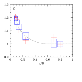
Figure 2: Inversion for the rotation profile for a model of $\epsilon$ Cep, a $\delta$ Scuti star. Data are the splittings computed for an input stellar model (1.8 $M_{\odot}$ main sequence star with $T_{eff}=7588K$ and a surface rotational velocity $v=120$km/s). The input prescribed rotation profile $\Omega$ normalized to its surface value is represented by dotted lines. Squares show the results of a SOLA inversion using the input model; crosses represent a SOLA inversion using a different model than the input one with a 1.90 $M_{\odot}$ mass and $T_{eff}=7906K$ with no rotation but with the same large separation $50\mu$Hz. from Goupil et al. 2000, unpublished)

Espinosa (2004) and Lignières et al. (2006) studied the effect of the centrifugal force. The first study chose an oblateness parameter in the range $\epsilon=0-0.3$ while the second one investigated the range $\epsilon=0-0.15;\Omega/\Omega_{k}=0$ up to 0.59 that-is a rotational velocity up to 150 km/s for a $\delta$ Scuti where $\Omega_{k}=({GM/R_{eq}^{3}})^{1/2}$ with $M$ the stellar mass and $R_{eq}$ the equatorial radius. The effects of the centrifugal force increase with increasing $\omega$ (Fig.2 of Lignières et al 2006). Frequencies of even and odd modes behave differently: frequencies of even modes tend to increase whereas those of odd modes decrease. The effect of the centrifugal force on p-modes is to contract the eigenfrequency spectrum. These effects are more important for high $n$ and low $\ell$ (see Fig.3 of Lignière et al 2006). Reese et al.  (2006) computed frequencies of a polytrope with a polytropic index $n=3$, using 70-80 $\ell$ degree spherical harmonics and 60-80 points for the radial grid in the spectral decompositions. Both the centrifugal and Coriolis forces are included. The Coriolis effects are found to decrease with increasing $\omega$. For high frequency modes, the effects du to the centrifugal force dominate. Visualisation of oscillations of a distorted rotating star can be seen on the web site of D. Reese or Fig.4 of Espinosa (2004).

Mode classification In general, the oscillation modes of a fast rotating star look like modes for a spherically symmetric star and a mode classification remains possible: the dominant $\ell$ degree most often corresponds to the degree of the mode for a zero rotation. This is shown by following the mode starting from a zero rotation and progressively increasing the rotation rate. However following the mode with increasing rotation rate is made more complicated by the presence of mixed modes. For the highest rotational velocities, the dominant degree $\ell$ is no longer the degree of the mode with zero rotation. The dominant $\ell$ can be as large as $\ell_{0}+6$ where $\ell_{0}$ is the degree of the mode for the nonrotating model. In that case, one can wonder whether the mode would still be visible in disk integrated light from ground? Would that contribute to explain the complicated patterns seen in power spectra of fast rotating $\delta$ Scuti stars where no frequency are detected in large domains in between frequency ranges where many frequencies are detected for the same star?

Mode pairing Espinosa (2004) found that the numerical frequencies computed assuming a uniform rotation and with the aforementioned approximation obey the relation $\omega_{n,\ell,m}=\bar{\omega}_{n,\ell,m}+m\Omega-f_{n,\ell}(m^{2},\Omega)-(-)^{\ell+m}g_{n,\ell}(m^{2},\Omega)$ where $f$ and $g$ are positive definite and monotonically increasing functions with $m^{2}$. The combined effect of the 3rd and last terms produces compressions of the frequencies within the multiplets which generate pairing of modes with different types of symmetry. Indeed for increasing rotation, frequencies tend to assemble by pair of modes with different values of $m$ (Fig.1 of Espinosa 2004, Lignières et al.  2006, Reese et al.  2006). This effect starts to appear for larger $\ell$ when the rotation is increased. The origin of such a pairing is attributed to the nonspherical distorsion of the structure. This effect might have already been observed in the Fourier spectra of $\delta$ Scuti star light curves.

New regularities in frequency spectra Fig.7.3 in PhD thesis of Reese (2006) shows that when the radial order $n$ increases, the large separation still tends toward a constant value but the small separation no longer decreases to 0 . Fig.7.2 also shows that the small separation between $\ell=0,n$ and $\ell=2,n-1$ modes for instance increases for increasing rotation as the frequency of the $\ell=2$ mode decreases whereas that of the radial one remains almost constant until some rotation is reached beyond which the small separation is now between the $\ell=2,n-1$ and the radial mode below ie $\ell=0,n-1$. This behavior is reminiscent of the avoided crossing behavior of the same modes when the (non-rotating) stellar model evolves i.e. with decreasing effective temperature or central hydrogen content. Reese et al. (2006a,b) modelled the behavior of the numerical frequencies as : $\omega_{n,\ell,m}=\Delta_{n}n+\Delta_{\ell}\ell-m\Omega+\Delta_{m}|m|+\alpha_{\pm}$ where the $\Delta$ coefficients are constant depending on $\Omega$ but not on $n,\ell,m$, $\alpha_{\pm}$ depends on $\Omega$ and on the $(\ell+m)$ parity of the mode.

Concentration of the amplitude toward the equator: The centrifugal distorsion is found to cause a high concentration of the mode amplitude toward the equator (Fig.8 of Lignière et al (2006)).

From a rotating polytrope to a more realistic stellar model Most of the above effects obtained for a polytrope appear to be also verified when one turns to the oscillation frequencies of a more realistic stellar model (Espinosa, 2004, PhD thesis). However, the effect of mode couplings seems to be stronger in the realistic case. This perhaps might be expected as the structure of a polytrope is smoother than that of a more realistic stellar model.

7.3 Validity of the results from perturbation techniques

From the previous chapter and what has been described in this chapter, one concludes that some results of perturbative and non pertubative methods are qualitatively similar. On the other hand, some new types of behavior seem to appear when the perturbative methods are no longer valid. For concrete studies, one then needs to quantify the domain of validity of perturbation methods. In order to do so, one must compare the results coming from the perturbation methods under the form Eq.120 with the numerical frequencies computed with a nonperturbative approach. Reese et al (2006) determined the dependence of the frequency $\omega$ in function of the rotation rate $\Omega$ by means of a polynomial fit of the form

$$\omega_{fit}(\Omega)=A_{0}+A_{1}~{}\Omega+A_{2}~{}\Omega^{2}+A_{3}~{}\Omega^{3}+O(\Omega^{4})$$

The $A_{j}$ coefficients are determined by fitting the numerical frequencies computed with the non perturbative approach. The authors then compared the numerical frequencies to their conterpart at a given level of approximation. The comparison is carried out with the differences $\delta_{j}=\omega-\omega_{app,j}$ where $\omega_{app,j}=\sum_{1}^{j}A_{j}\Omega^{j}$ . When only the centrifugal force in included, the error between second order perturbative and nonperturbative frequencies is $\sim 11\mu$Hz for $\Omega/\Omega_{K}=0.24$ for a typical delta Scuti star with a rotational velocity of 100 km/s (Fig.12, Lignières et al 2006). The relative error reaches $3\%$ at $\Omega/\Omega_{K}=0.3$. Reese et al.(2006) considered more appropriate quantities for the comparison:

$${\omega_{n,\ell,m}+\omega_{n,\ell,-m}\over 2} =\omega^{0}_{n,\ell,m}+\omega^{2}_{n,\ell,m}\Omega^{2}+\omega^{4}_{n,\ell,m}\Omega^{4}$$ (139)

$${\omega_{n,\ell,m}-\omega_{n,\ell,-m}\over 2} =\omega^{1}_{n,\ell,m}\Omega+\omega^{3}_{n,\ell,m}\Omega^{3}+\omega^{5}_{n,\ell,m}\Omega^{5}$$ (140)

Frequency differences between perturbative and nonperturbative computations are the same for two modes with opposite $m$ and same $\ell,n$. Reese et al.(2006) found that the error which is introduced between perturbative frequencies and non perturbative ones is larger than the accuracy of frequency measurement (0.4 $\mu$Hz) for 150 days of observation for a solar like oscillating star. (0.08 $\mu$Hz) (Fig.4 of Reese et al 2006). In the frequency range considered and with COROT’s accuracy, it is found that complete calculations are required beyond $vsini=50kms^{-1}$ for a $R=2.3R_{\odot},M=1.9M_{\odot}$ polytropic star. Furthermore, it is shown that the main differences between complete and perturbative calculations come essentially from the centrifugal distortion. A comparison between the results of nonperturbative calculations and those from perturbative computations as described in the previous section is also necessary and is currently being carried out.

8 Observed rotational splittings and forward inferences

8.1 Solar-like pulsators

Several low to intermediate mass main sequence stars are known to oscillate with solar like oscillations. However, they are rotating too slow and in all but one instance and apart for the Sun, their splittings have not been detected yet.

$\alpha$ Cen A :

50 days of space photometric observations of this star with Wire led to the detection of 18 frequencies in the range 1700-2650 $\mu$Hz which were measured with an accuracy of 1-2 $\mu$Hz (Fletcher et al. 2006). Detected modes have $\ell=0$ to 2 and radial order $n=14-18$. These observations allowed to determine an average value for the rotational splitting of $0.54\pm 0.22\mu$Hz.

Procyon:

Solar like oscillations for Procyon have been detected in velocity measurements (Claudi et al. 2005, Leccia et al.  2007, Heeker et al.  2007). Some controversy exists as to whether these oscillations can be detected in photometry even from space. As a prototype for a 1.5 $M_{\odot}$ main sequence star, Bonanno et al. (2007) have modelled the latitudinally differential rotation in the outer convective layers for this star. Their models give a flatness of order 0.1-0.45 which is comparable with the solar case 0.25. The authors computed a latitudinal averaged $\Omega(r)$. The splittings differ by a few nanoHz depending on the latitudinal shear obtained in the models generating the differential rotation. Such a small value could be detected with Corot after averaging over several multiplets.

HD 49933:

The space experiment Corot, which was successfully launched in december 2006, seems to be able to keep its promises and makes possible to detect mean splitting values as well as individual splittings at least in some favorable cases. As the first solar-like target for this mission, HD49933 was observed from ground with the spectrograph HARPS (Mosser et al, 2005). These observations confirmed the expectation that this star is a solar like oscillator. The star shows a high degree of stellar activity and the rotation appears to be quite rapid with a period of the order of 4-8 days. The star was the object of a hare and hound exercise in order to see whether splittings can indeed be detected and which accuracy can be expected. This exercice indicated that for an assumed rotation of 1.4-2.9$\mu$ Hz, many splittings could be detected. Only a few correct ones however were measured within $0.5\mu$Hz from the correct value and with error bars less that $0.5\mu$Hz (Appourchaux et al. 2006).

8.2 $\delta$ Scuti stars

These stars are nonradial multiperiodic variables with excited modes in the vicinity of the fundamental. The main problem for these stars is mode identification. As it is not yet possible to assign $n,l,m$ values with full confidence to the observed frequencies, it is difficult to get information on the star. As far as rotational splitting is concerned, a few detections have been claimed:

GX Peg

belongs to a spectroscopic binary system. Knowing the surface rotation from the binarity, the identification of a splitting led to the conclusion that the core is rotating faster than the outer layers (Goupil et al.  1993). The rotationally split multiplet was found asymmetric which could be attributed to distorsion of the star by the centrifugal force.

FG Vir

is one of the best studied delta Scuti star. Its variability has been extensively observed and analysed and the results have been the subject of many observations and theoretical studies over the past 20 years (Breger et al. 2005; Pamyatnykh, Daszynska-Daskiewicz et al.  2005; Zima et al.  2006). Among about 70 detected frequencies, a dozen $\ell$ and $m$ values can be assigned. The star appears to be moderately rotating with a equatorial velocity of $66\pm 16km/s$. Most of the identified modes are axisymmetric but Zima et al.  (2006) found that one $\ell=1$ triplet is observed with a splitting value of 6.13 $\mu$Hz. Failure to find a stellar model which frequencies match the observed frequencies of FG Vir subsists even when taking into account second order rotational effects.

44 Tauri

has been observed for a long time and is known to pulsate with at least 13 frequencies. Mode identification indicates a few possible splitting components among them which indicate that the star is a slow rotator with 26 km/s as an equatorial velocity (Poretti et al.  1992, Antoci et al.  2006 and references therein).

HD104237:

Detecting the rotational splittings of oscillating PMS stars ought to be relatively easy as they are fast rotators and their power spectra are expected to be much simpler than those of their postZAMS counterparts i.e. delta Scuti stars (Suran et al. 2001). Determining their rotation profiles and internal structures can give us clues about temporal evolution of rotation profiles and transport of internal angular momentum. In this spirit, the binary PMS system HD104237 is being studied as one of its two components has been identified as a $\delta$ Scuti star (Alecian et al.  2005, 2007; Goupil et al.  2005 ; Dupret et al.  2006).

8.3 $\beta$ Cephei stars:

More massive than $\delta$ Scuti stars, B-type main sequence stars oscillate with periods between 1.5 h and 8 h corresponding to low radial order p and g -modes. Their projected rotational velocities can reach up to 300 km/s. Rotational splittings for $\ell=1$ and $\ell=2$ modes seem to have been detected for a few stars (see for instance Fig.1 of Pigulski, 2007).

HD129929, a $\sim 8-9M_{\odot}$ $\beta$ Cephei star:

This star is known to oscillate with at least 6 identified frequencies. From one $\ell=1$ multiplet, the rotational splitting yields a rotational velocity of 3.61 km/s when assuming a uniform rotation. On the other hand, 2 successive components of a $\ell=2$ multiplet indicate a rotational velocity of 4.20 km/s. This leads to the likely conclusion that the rotation varies with depth with a ratio of the angular velocity at the center to that the surface $\Omega_{c}/\Omega_{s}=3.6$ (Dupret et al. 2004).

$\nu$ Eridani

is another $\beta$ Cepheid which shows a rich frequency spectrum but with only a few of them identified (see Fig. 1 of Ausseloos et al.2004). Pamyatnykh et al.(2004) used the identified $\ell=1$, $g1$ triplet and two components of the $\ell=1$, $p1$ to determine a non uniform rotation for this star with $\Omega_{c}/\Omega_{s}\sim 3$, close to what is found for HD 129929. Using an assumed depth dependent profile, Suarez et al (2007) computed the splittings and their associated departures from equidistant in order to reproduce the observed 3 $\ell=1$ multiplets obtained by Jerzykiewicz et al (2005). The observed asymmetries are in favor of a non uniform rotation profile although they are too small to allow a definitive conclusion.

$\theta$ Ophuichi

is a $\sim 8-9M_{\odot}$ $\beta$ Cepheid with 7 identified frequencies (Handler et al., 2005): a $\ell=1,p1$ triplet and 4 components of a $\ell=2,g1$ quintuplet (Fig.6 of Handler et al., 2005). The splittings indicate a rotation velocity of $29\pm 7$ km/s, large enough to cause detected departure from equal splittings (Briquet et al. 2007).

9 Inversion for rotation

We consider the simplified problem of determining the depth dependent rotation law of a star from the measurements of its rotational splittings. For more general 2D inversions which yields $\Omega(\theta,r)$ as well as for more details on inversion methods and results on the solar internal rotation, we refer the reader to general such as reviews Gough (1985); Gough & Thompson, (1991), Thompson et al.(2003).
According to Eq.60, a 1D rotation profile is related to the splittings by the integral relation

$$\delta\omega_{j}+\delta(\delta\omega_{j})=\int_{0}^{R}~{}K_{j}(r)~{}\Omega(r)dr$$ (141)

where for shortness $j$ represents the set of values $(n,\ell)$ and $\delta(\delta\omega_{j})$ is the incertainty pf the measured splitting values. In general, only a finite number, $N$, of discrete splittings values associated with $N$ modes, are available. The measurements are polluted with some observational errors $\delta S_{j}$ which are assumed uncorrelated with a variance $\sigma_{j}^{2}$. In order to derive the rotation profile from the observed splittings, one must invert the relation Eq.141. As the data are related to the rotation profile by a linear functional, one is confronted to a linear inverse problem.

9.1 Splittings of high frequency p-modes and the Abel equation

For modes with high radial orders or degrees, the eigenfunctions vary more rapidely than the equilibrium quantities; hence the scale of spatial variations of the eigenfunctions being smaller than that of the basic state, a local analysis is valid. One then assumes that the solution can be cast under the form of a plane wave: $\vec{v^{\prime}}\propto e^{i(\omega t-\vec{k}\cdot\vec{r})}$ with $\vec{k}$ the wavenumber and $|\vec{k}|^{2}=k_{r}^{2}+k_{h}^{2}$, with $k_{r},k_{h}$ the radial and horizontal components. One can also neglect the perturbation of the gravitational field (Cowling approximation) as well as the derivatives of the equilibrium quantities. For high frequency p-modes which nature is mainly acoustic, the eigenfrequency is much larger than the Brünt-Väissälä frequency ($\omega^{2}>>N^{2}$) which therefore can be neglected in the problem considered here. With these approximations, one recovers the expected dispersion relation for an acoustic wave $\omega^{2}=k^{2}~{}c_{s}^{2}$ where $k^{2}=k^{2}_{r}+k^{2}_{h}$ and $k_{h}={S^{2}_{\ell}/c_{s}^{2}}={\Lambda/r^{2}}$ with $\Lambda=\ell(\ell+1)$ and $c_{s}(r)$ is the adiabatic sound speed profile, $S_{\ell}^{2}={c^{2}_{s}\Lambda/r^{2}}$ is the squared Lamb frequency. One then has:

$$k^{2}_{r}(r)\approx{1\over c_{s}^{2}}(\omega^{2}-S_{\ell}^{2})={\omega^{2}\over c_{s}^{2}}-{\Lambda\over r^{2}}$$

Let recall first that for a 1 dimensional acoustic wave with a wavenumber $k$ with a node at one end ($r=0$) and a free boundary at the other end ($r=R$), the resonant condition for the existence of a normal mode in a homogeneous medium is $kR=n\pi-\pi/2$ for some integer $n$. In the stellar 3D (inhomogeneous) medium, this condition becomes

$$\int^{R}_{r_{t}}~{}k_{r}(r)~{}dr=(n-{1\over 2})\pi$$ (142)

where $r_{t}$ is the radius of the mode inner turning point.

Taking for the mode frequency, the frequency corrected for the first order effect of rotation, $\omega\sim\omega_{0}+(\delta\omega+m\Omega)$ where $\omega_{0}$ is the zeroth order frequency (ie the frequency of the mode in abscence of rotation), one obtains

$$k_{r}(r)={\cal Q}+\left({\omega^{(0)}\over c_{s}^{2}{\cal Q}}\right)(\delta\omega+m\Omega)$$

with

$${\cal Q}=\left({\omega^{(0)2}\over c_{s}^{2}}-{\Lambda^{2}\over r^{2}}\right)^{1/2}={\omega^{(0)}\over c_{s}}\left(1-{a^{2}\over W^{2}}\right)^{1/2}$$

and $a=c_{s}(r)/r$ et $W=\omega_{0}/\Lambda$. Recalling that at zeroth order, one has

$$\int_{r_{t}}^{R}{\cal Q}(r)dr=(n-{1\over 2})\pi~{}~{}~{}~{}~{}~{}~{}~{}~{},$$

the resonant condition Eq.142 becomes:

$$\delta\omega={1\over S}~{}\int^{R}_{r_{t}}~{}m~{}\Omega(r)\left(W^{2}-a^{2}\right)^{-1/2}~{}{dr\over c_{s}}$$ (143)

with

$$S=\int^{R}_{r_{t}}\left(W^{2}-a^{2}\right)^{-1/2}~{}{dr\over c_{s}}$$

Note that for very high radial order modes, $a/W<<1$ and

$$\delta\omega=m~{}\int_{r_{t}}^{R}\Omega(r){dr\over c_{s}}~{}\left(\int_{r_{t}}^{R}{dr\over c_{s}}\right)^{-1}$$ (144)

which shows that the perturbation of the frequency by the rotation can be expressed as an average of the rotation weighted by the acoustic propagation time in the radial direction inside the cavity.
Eq.143 is of Abel type. Indeed the Abel (integral) equation is defined as:

$$\int_{0}^{x}{f(y)\over(x-y)^{\alpha}}dy=g(x)~{}~{}~{}~{}~{}0<\alpha<1~{}~{}~{}g(0)=0$$ (145)

and has the formal solution (Gough, 1985):

$$f(y)={1\over\pi}\sin(\pi\alpha){d\over dx}\int_{0}^{y}{g(x)\over(y-x)^{1-\alpha}}dx$$ (146)

Eq.143 then admits an analytical inverse solution. The angular velocity is given by:

$$\Omega(r)=-{2a\over\pi}{d\over d\ln r}\int_{a_{s}}^{a}(a^{2}-W^{2})^{-1/2}{\cal H}(W)dW$$ (147)

where $a_{s}=a(R)$ and ${\cal H}(w)$ represents the data set derived from the observed splittings.

The Abel equation, Eq.145, is known to be an ill-posed inverse problem in the sense of Hadamard (1923). The existence of an analytical solution to the inverse problem does not suppress the ill-posed nature of the numerical inversion, particularly when the observational data are noisy.

Ill-posed nature of an inverse problem

A well-posed problem in the sense of Hadamard (1923) is defined as follows: let consider the equation ${\cal H}(f)=g$ where ${\cal H}$ is an operator $\in{\cal F}\longrightarrow{\cal O}$ where ${\cal F}$ et ${\cal O}$ are closed vectorial spaces and more specifically here the integral equation:

$$\int_{0}^{R}K(x,y)f(y)dy=g(x)$$ (148)

The three Hadamard conditions are :

- existence of a solution: $\forall g\in{\cal O}$, $\exists f\in{\cal F}$ such that ${\cal H}(f)=g$

- unicity of the solution: $\forall g\in{\cal O},\exists$ at most one $f\in{\cal F}$ such that ${\cal H}(f)=g$

- stability of the solution with respect to the data: $\forall f_{n}$, any sequence $\in{\cal F}$ such that

$$\lim_{n\rightarrow+\infty}{\cal H}(f_{n})={\cal H}(f)~{}~{}~{}~{}~{}~{}~{}{\rm then}~{}~{}~{}~{}~{}\lim_{n\rightarrow+\infty}f_{n}=f$$

This last condition can be understood in a more practical sense as

$$|{\delta g\over g}|<<1\rightarrow|{\delta f\over f}|<<1$$

Existence and unicity are the classical conditions for solving an equation and the stability condition, on the other hand, is an additional condition which requires that, for a well-posed problem, any small perturbation of the data can only lead to a small error on the solution. This condition is barely verified in practice for inverse problems. In particular, inversions of integral equations often are ill-posed problems: noise, even small, in the data can cause the derived solution to be very far from the true one.

Nonuniqueness and sensitivity to noise

One must recall that the inverse problem Eq.148 admits the set of solutions $f(y)+h(y)$ provided that
$\int_{0}^{R}K(x,y)h(y)dy=0$

Furthermore, the Riemann-Lebesgue theorem states that:

$$~{}\int_{a}^{b}K(x,y)\cos(my)dy=0~{};~{}\int_{a}^{b}K(x,y)\sin(my)dy=0$$

when $m\rightarrow\infty$, valid for any integrable $K(x,y)$. Consequences:

i) on one hand, high frequency components of the solution $f(y)$ are not accessible as they are smoothed by the kernel $K(x,y)$ to an arbitrary small amplitude level in the data. As an illustration, let some perturbation of the source function $f$ in Eq.145, be of the form: $\delta f(y)=A\sin(2\sqrt{\lambda y})$ (Craig & Brown, 1986). It causes a perturbation of the data of the form:

$$\delta g(x)=A\sqrt{\pi}\Gamma(1-\alpha)\lambda^{\beta}x^{(3/2-\alpha)/2}J_{3/2-\alpha}(2\sqrt{\lambda y})$$ (149)

where $\beta=(\alpha-1/2)/2$ and $J_{3/2-\alpha}$ is a Bessel function of 1st kind of order $3/2-\alpha$. For high frequencies (i.e. $\lambda\longrightarrow\infty$), one can use $|J_{\nu}(z)|\sim|{2/\pi z}|^{1/2}$ and Eq.149 becomes $|\delta g(x)|\sim\Gamma(1-\alpha)\lambda^{(\alpha-1)/2}x^{(1-\alpha)/2}$ so that for any amplitude $A$ and $\forall\alpha<1$, $\delta g(x)\longrightarrow 0$ when $\lambda\longrightarrow\infty$. Any discontinuity can be represented by an infinite Fourier series but all the high frequency components are smoothed out and contribute to the data at a small amplitude level; they can not be distinguished from the high frequency noise in the data. The smoothing properties of the operators and/or kernels in the process $f\rightarrow g$ remove any real discontinuity of the solution $f$ and which is therefore difficult, if not impossible, to bring out from the data.

ii) on the other hand, high frequency small perturbations in the data (noise) appear as large amplitude oscillating components in the calculated source. These large amplitude contributions can dominate the inverse solution even if they are totally spurious as due to small perturbations in the data due to noise. An exemple given by Craig & Brown (1986) illustrates this issue (cf Fig.1). One considers the particular kernel $K(x,y)=1$ in Eq.148 (differentiation). Let 2 functions $g_{1}(y)$ et $g_{2}(y)$ differing only by the addition of a sinusoidal component with a given frequency $\Delta g$. We choose for instance $g_{1}(x)=1-e^{-\alpha x}~{}~{};~{}~{}g_{2}(x)=g_{1}(x)+\beta\sin\omega x$. The difference appears in the source functions $f_{1}$ and $f_{2}$ as $\Delta f(y)=f_{2}(x)-f_{1}(x)=\omega\beta\cos\omega y$. Fig.1 shows the data and the source functions for $\alpha=0.8;\beta=0.04;\omega=20$. Although the difference $g_{1}-g_{2}$ is very small, the corresponding difference in the source functions is an oscillatory behavior with a large amplitude.

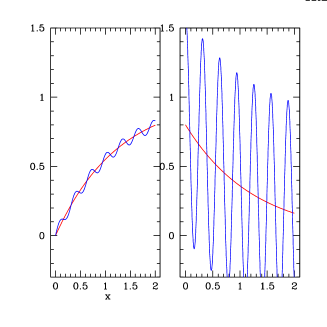
Figure 1: The left pannel displays the noise free data function $g1$ and the slightly noisy data function $g2$ where the perturbed part is represented by a small (5 %) amplitude oscillation. The right pannel shows the true inverse solution, $f1$, and the inverse solution of the noisy function $g2$, $f2$, which is dominated by a spurious large (100 %) amplitude oscillation (adapted from Craig & Brown (1986)).

Hence since observations cannot in general be noise free, a simple ’ naive’ inversion is not able to give the correct inverse solution.

Discretisation and a measure of the ill-posed nature of the problem

Although the first inversions for the solar rotational splittings using Eq. 143 were successfull enough, the asymptotic integral relation remains an approximation. In practice, one actually considers the general relation Eq.59 and inversions are carried out first by discretizing the integral. Let write the resulting discretized relation as : $\Delta=AX$ where $\Delta$ represents the data vector and $X$ is the rotation vector to be determined. The stability can be measured with the conditionning of the matrix $A$. If $A$ is regular, its conditionnement is defined as $cond(A)=||A||~{}||A^{-1}||$ where $||A||$ is a matrix norm for close $A$. Note that $cond(A)\geq 1$ is always verified. A well conditionned matrix is such $cond(A)$ remains close to 1. Using the norm $||A||=max_{j}(\mu_{j})$ where $\mu_{j}$ are the singular values of $A$ (i.e. the square root of the eigenfrequencies of the squared symmetric matrix $AA^{t}$), one shows that $cond(A)={\mu_{max}/\mu_{min}}$. A small perturbation $\delta\Delta$ of the data generates a perturbation $\delta X$ of the solution then $\delta\Delta=A(\delta X)$ and it is easy to deduce from the matrix norm properties that

$${||\delta X||\over||X||}\leq cond(A){||\delta\Delta||\over||\Delta||}$$

Accordingly, if $A$ is well conditionned ($cond(A)\sim 1$), the stability condition is satisfied whereas for $condA>>1$ which is most often the case, $||\delta X||$ can become large compared with $||X||$ and the problem is ill-posed.

Once the ill-posed nature of the inverse problem is recognized, one is then force to carry out a regularization of the calculated solution. As seen above, helio- and astero- seismic inversions are ill-posed problems which therefore require regularisation inverse techniques.

9.2 Inversion with regularisation

Several classes of inversion techniques with regularisation exist. They are based on the addition of a priori information on the solution, often on the shape of the solution. One wants a solution which remains insensitive to errors in the data. Most methods involve one or two parameters which control the sensitivity of the solution to errors in the data. We briefly present two of the most currently used ones in the stellar context.

Inverse methods with a priori douceur or Tikhonov’s methods :

The inversion strategy consists in determining a solution where high frequency variations -which cannot be identified as real or due to noise magnification- have been removed. One then seeks for a global solution which reproduces at best the data without reproducing the noise (seen as the high frequency components). The procedure is to find a least square solution submitted to a regularisation constrain : $min(||AX-\Delta||^{2}+\gamma~{}\sigma^{2}~{}B(X))$ where $\sigma$ is the variance of the noise and $\gamma$ a trade-off parameter and $B$ a discretized regularising function. This is equivalent to solve the normal form equation: $(A^{t}A+\gamma B^{t}B)X=A^{t}\Delta)$ where $A^{t}$ is the transposed matrix. The regularising function $B(X)$ is often taken as the second derivative of the solution since one wishes to eliminate the high frequency part of the solution. The trade-off parameter $\gamma$ must be adjusted to realize the best compromise between a noise insensitive but distorted solution (large $\gamma$) and a solution which is not regularised enough (small $\gamma$).

Optimally Localized averages: OLA and its variants

One looks for a local solution that-is- an averaged value of the solution over a small interval about a given radius. The SOLA method is a variant of the OLA technique (Backus & Gilbert 1970) developed by Pijpers and Thompson (1992, 1994, 1996). It aims at building localised kernels ${\cal K}$ about a predefined value, $r=r_{0}$ as linear combinations of the rotational kernels $K_{j}(r)$: ${\cal K}(r,r_{0})=\Sigma_{j}c_{j}(r_{0})~{}K_{j}(r)$. The coefficients $c_{j}$ must be determined by a minimisation process:

$$min_{cj}(|\int({\cal K}-T)^{2}~{}dr|^{2}+\gamma E^{2})$$

where $T(r,r_{0})$ is a predefined target, $E$ is the noise covariant matrix; $\gamma$ a trade-off parameter in order to obtain a satisfying compromise between magnification of the error and the width of the target ie the interval over which the solution is averaged. The SOLA method with a predefined target presents the advantage over the original OLA method that the inverse matrix is computed once and for all. Once the $c_{j}(r_{0})$ are determined, one computes the average rotation value as $<\Omega(r)>_{r0}=\sum_{j}c_{j}(r_{0})~{}\delta\omega_{j}$. Indeed one has

$$\sum_{j}c_{j}(r_{0})\delta\omega_{j} = \sum_{j}c_{j}(r_{0})(\int K_{j}(r)\Omega(r)dr)$$ (150)

$$= \int(\sum_{j}c_{j}(r_{0})K_{j}(r))\Omega(r)dr$$ (151)

$$= \int{\cal K}(r,r_{0})\Omega(r)dr\sim\int T(r,r_{0})\Omega(r)dr$$ (152)

If the target $T$ is a Dirac function i.e. $T=\delta(r-r_{0})$ , then $\sum_{j}c_{j}\delta\omega_{j}=\Omega(r_{0})$. However one seldomely has enough information in the data to succeed in building Dirac function as localised kernels. Usually the target function takes the form of gaussian with a given width. Again a compromise must be obtained between the magnification of the error and the width of the target ie the interval over which the solution is averaged.

9.3 Application to stellar seismology

The solar rotation profile

With the high quality helioseismic data available for the past 2 decades or so, highly accurate frequency splittings were obtained and allowed to derive the 2D rotation profile in the 3/4 outer part of the Sun. See Fig.5 of Schou et al.  (1998) for instance for the result of an inversion based on SoHo data. Several 2D inversion methods have been applied with various adjustements and adaptations to the available helioseismic data sets over the years (Schou et al.  (1994ab, 1998), Antia et al. (1998)). This has provided the internal rotation profile for the Sun with quite a number of surprises at the time: latitudinal dependence of rotation in the convective outer region and uniform rotation in the radiative region. Only the rotation of the inner part is still not yet accessible.

The inversion results have generated many studies in order to explain these seismic results. Several studies have led to identify the shear of the Reynolds stress as responsible for differential rotation in latitude in the convective outer layers of the Sun; others have studied the importance and the role of the tachocline in the solar magnetogydrodynamical processes, see for instance Rüdiger et al.  2003, 2005; Miesch et al.  2007, Zahn et al. 2007.

The discovery of the uniform rotation of the solar radiative zone drove the developement of models able to transport angular momentum from the inner to the outer part. It was found type I rotationally induced mixing models are not efficient enough and predict an incorrect increase of the rotation rate with decreasing radius (Talon et al.  1997; Matias & Zahn, 1998)). Internal waves, on the other hand, are very efficient in transporting the angular momentum from center upward to the surface and inforce a uniform rotation in the radiative zone. (Charbonnel & Talon , 2005; Talon, 2006 and references therein). Fig.1 of Charbonnel Talon (2005) shows the evolution of the rotation profile for a $1.2M_{\odot}$ stellar model from 0.2 Gyrs up to 4.8 Gyrs when rotational induced mixing of type I is included and the successful approach of uniform rotation when mixing of type II is included.

One current issue is the role of the magnetic field, another is to determine to what extent these results and explanations are valid for other stars than the Sun, particularly young stars which rotate faster than the Sun. In that context, information from 3D simulations will be of great help (Brun et al.  2006, Ballot et al.  2007).

Solar like stars

The observed high frequency solar p- modes do not give access to the core rotation. For stars slightly more massive and slightly more evolved than the Sun such as $\eta$ Boo for instance, a small number of mixed modes does indeed exist in the high frequency domain of modes excited by the turbulent convection of the outer layers. A theoretical study was carried out with SOLA inversions for the rotation profile on simulated data for a 1.5 $M_{\odot}$ stellar model with a surface velocity of $\sim 30$ km/s and a ratio between the rotation rate at the center to that at the surface $\Omega_{c}/\Omega_{s}\sim 3$ (Lochard et al.  2005). The incertainties were estimated in function of the expected Corot performances. Fig.8 of Lochard et al.  (2005) shows that the variation for the rotation profile with radius in the vicinity of the convective core - varying from $\Omega/\Omega_{s}=1.5$ at $r=0.2$, (with a incertainty on the recovered value $\pm 0.2$) to $\Omega/\Omega_{s}=2.4$ at $r\leq 0.1$ (with a incertainty on the recovered value $\pm 0.6$)- is accessible.

Inversion for rotation for $\delta$ Scuti like oscillations

Other stars oscillate with modes with lower frequencies in the vicinity of the fundamental, driven by an opacity mechanism. These stars are slightly more massive than the Sun and develope a convective core on the main sequence which receeds with time. This generates the existence of mixed modes in the excited frequency range. Only one or two such modes are enough to give access to $\Omega_{c}$ the core rotation rate (Goupil et al. 1996). One illustrative exemple is $\epsilon$ Cep. Assuming that one has obtained a seismic model for this star that-is a model as close as possible of reality with the same mean large separation, a SOLA inversion was performed with a data set of $\ell=1,6$ linearly unstable modes. The variation of the rotation profile with depth is well recovered.

This theoretical study assumed a noise level according to Corot performances. The inversion was carried out with linear splittings Eq.60 although for a real case, distorsion effects on the splittings ought to be included for such a moderately rapid rotator ($v~{}\sin i=91$km/s, Royer et al.  2002). Several frequencies have recently been detected for this star but its complex frequency pattern has not yet been fully elucidated (Bruntt et al.  2007).

References

- (1) Alecian, E. and Catala, C. and van’t Veer-Menneret, C. and Goupil, M.-J. and Balona, L., 2005, AA 442, 993
- (2) Alecian, E. and Goupil, M.-J. and Lebreton, Y. and Dupret, M.-A. and Catala, C., 2007, AA 465, 241
- (3) Antia, H. M. and Basu, S. and Chitre, S. M., 1998, MNRAS 298, 543
- (4) Antoci, V., Breger, M., Bishof, K., Garrido, R., 2006, PASP 349, 181, eds. C. Sterken, C. Aerts
- (5) Appourchaux, T. and Berthomieu, G. and Michel, E. et al. , 2006, ESA Special Publication, vol. 1306, p. 377
- (6) Ausseloos, M. and Scuflaire, R. and Thoul, A. and Aerts, C., 2004, MNRAS, 355, 352
- (7) Backus, G. & Gilbert, F., 1970, Phil. Trans. R. Soc. London, A 266, 123
- (8) Baglin, A., Auvergne, M., Barge P. Deleuil, M., Catal, C. Michel, E., Weiss, W., and the CoRoT team, 2006, ESA Special Publication, vol. 1306, 33
- (9) Ballot, J. and Brun, A. S. and Turck-Chièze, S., 2007, ApJ 669, 1190
- (10) Bonazzola, S. and Gourgoulhon, E. and Marck, J.-A., prd, arXiv:astro-ph/9803086, 58,
- (11) Bonanno, A. and Küker, M. and Paternò, L., 2007, AA 462, 1031
- (12) Breger, M. and Lenz, P. and Antoci, V. et al. , 2005, A&A, 435, 955
- (13) Briquet, M. and Morel, T. and Thoul, A. and Scuflaire, R. and Miglio, A. and Montalbán, J. and Dupret, M.-A. and Aerts, C., 2007, MNRAS 381, 1482
- (14) Brun, A. S. and Miesch, M. S. and Toomre, J., 2006, ArXiv Astrophysics e-prints, astro-ph/0610073
- (15) Bruntt, H., Suarez, J.C. , Bedding, T.R., et al., 2007, AA 461, 619
- (16) Burke, K. D. and Thompson, M. J., 2006, in Proceedings of SOHO 18/GONG 2006/HELAS I, Beyond the spherical Sun, ESA Special Publication, 624,
- (17) Buzasi, D. L. and Bruntt, H. and Bedding, T. R. et al. , 2005, AA 619, 1072
- (18) Chaboyer, B. and Zahn, J.-P., 1992, AA 253, 173
- (19) Chandrasekhar, S. and Lebovitz, N. R., 1962a, ApJ 136, 1069
- (20) Chandrasekhar, S. and Lebovitz, N. R., 1962b, ApJ 136, 1082
- (21) Chandrasekhar, S. and Lebovitz, N. R.,1962c, ApJ 136, 1105
- (22) Chandrasekhar, S., 1964, ApJ 140, 599
- (23) Chandrasekhar, S. and Lebovitz, N.R., 1968, ApJ 152, 152
- (24) Charbonnel, C. and Talon, S., 2005, Science, 309, 2189
- (25) Charbonneau, P., 1992, AA 259, 134
- (26) Chlebowski, T.,1978, Acta Astronomica, 28, 441
- (27) Christensen-Dalsgaard, J. and Mullan, D. J., 1994, MNRAS 270, 921
- (28) Christensen-Dalsgaard, J. and Thompson, M. J., 1999, AA 350, 852
- (29) Christensen-Dalsgaard, J., 2003 (CD03), Lecture Note on Stellar Oscillation, 5th edition, http://www.phys.au.dk/ jcd/oscilnotes/)
- (30) Claudi, R. U. and Bonanno, A. and Leccia, S. et al. , 2005, AA 429, L17
- (31) Clement, M. J., 1965a, ApJ 141, 210
- (32) Clement, M. J., 1965b, ApJ 142, 243
- (33) Clement, M. J., 1981, ApJ 249, 746
- (34) Clement, M.J., 1984, ApJ 276, 724
- (35) Clement, M. J., 1989, ApJ 339, 1022
- (36) Cowling, T. G. and Newing, R. A., 1949, ApJ 109, 149
- (37) Cox, J. P., 1980 , ”Theory of stellar pulsation”, Research supported by the National Science Foundation Princeton, NJ, Princeton University Press
- (38) Craig, I.J.D, Brown, J.C., 1986, Inverse problems in Astronomy, Ed Adam Hilger Ltd
- (39) Daszynska-Daszkiewicz Dziembowski, W.A., Pamyatnykh, A.A., Goupil, M.J., 2002, AA 392, 151
- (40) Daszynska-Daszkiewicz, J., Dziembowski, W.A., Pamyatnykh, 2003, AA 407, 999
- (41) Deupree, R. G., 1990, ApJ 357, 175
- (42) Deupree, R. G., 2001, ApJ 552, 268
- (43) Domiciano de Souza, A. and Kervella, P. and Jankov, S. et al. , 2005, AA 442, 567
- (44) Dupret, M.-A. and Thoul, A. and Scuflaire, R. et al. , 2004, AA 415, 251
- (45) Dupret, M.-A. and Böhm, T. and Goupil, M.-J. et al. , 2006 Communications in Asteroseismology 147, 72
- (46) Dyson, J. and Schutz, B. F., 1979, in Royal Society of London Proceedings Series A, 368, 389
- (47) Dziembowski, W. A. and Goupil, M.-J., 1998, in The First MONS Workshop: Science with a Small Space Telescope, held in Aarhus, Denmark, June 29 - 30, 1998, Eds.: H. Kjeldsen, T.R. Bedding, Aarhus Universitet, p. 69., eds. Kjeldsen, H. and Bedding, T. R., p. 69
- (48) Dziembowski, W. A. and Goode, P. R., 1992 (DG92), ApJ 394, 670
- (49) Eddington, A. S., 1929, MNRAS 90, 54
- (50) Eggenberger, P., Carrier, F., 2006, AA 449, 293
- (51) Espinosa, F. , 2004, PhD thesis
- (52) Espinosa, F. and Pérez Hernández, F. and Roca Cortés, T., 2004 in SOHO 14 Helio- and Asteroseismology: Towards a Golden Future, ESA Special Publication, vol. 559, ed. Danesy, D., p. 424
- (53) Espinosa Lara, F. and Rieutord, M., AA 470, 1013
- (54) Fletcher, S. T. and Chaplin, W. J. and Elsworth, Y. and Schou, J. and Buzasi, D., 2006, MNRAS 371, 935-944
- (55) Gough, D., 1985, Sol. Phys 100, 65
- (56) Gough, D. O. and Thompson, M. J., 1990 (GT90), MNRAS 242, 25
- (57) Gough, D.O., Thompson, M.J., 1991, ‘The inversion probleme, in Solar interior and atmosphere Eds A.N. Cox; W.C. Livingston, M.S. Matthews, University of Arizona Press p. 519
- (58) Gough, D.O., 1993, ‘Linear adiabatic stellar pulsation’, in Astrophysical fluid fluid dynamics, Les Houches Session XLVII 1987, Eds J.P. Zahn, J. Zinn-Justin, Elsevier Science Publishers B.V., p. 399
- (59) Goupil, M. J. and Michel, E. and Lebreton, Y. and Baglin, A. , 1993, AA 268, 546
- (60) Goupil, M. J. and Michel, E. and Cassisi, S. et al. , 1995, IAU Colloq. 155: Astrophysical Applications of Stellar Pulsation, Astronomical Society of the Pacific Conference Series, 83, eds Feast, M. W., 453
- (61) Goupil, M.-J. and Dziembowski, W. A. and Goode, P. R. and Michel, E., 1996, AA 305, 487
- (62) Goupil, M.-J. and Dziembowski, W. A. and Pamyatnykh, A. A. and Talon, S., 2000 in Delta Scuti and Related Stars, Astronomical Society of the Pacific Conference Series, 210, eds. Breger, M. and Montgomery, M., p. 267
- (63) Goupil, M. J. and Talon, S., 2002, in IAU Colloq. 185: Radial and Nonradial Pulsations as Probes of Stellar Physics, Astronomical Society of the Pacific Conference Series, 259, eds Aerts, C. and Bedding, T. R. and Christensen-Dalsgaard, J. , 306
- (64) Goupil, M. J. and Samadi, R. and Lochard, J. et al. , 2004, in Stellar Structure and Habitable Planet Finding, ESA Special Publication, 538, eds Favata, F. and Aigrain, S. and Wilson, A., 133
- (65) Goupil, M.-J. and Dupret, M. A. and Samadi, R. and et al. , 2005, JApA vol. 26, 249
- (66) Goupil, M. J. and Moya, A. and Suarez, J. C. and et al. , 2006, ESA Special Publication, vol. 1306, p. 51
- (67) Goupil, M. J. and Dupret, M. A.,2007, EAS Publications Series, 26, 93
- (68) Hadamard J., 1923, ’Lectures on Cauchy’s Problem in Linear Partial Differential Equations’, (New Haven, CT: Yale University Press)
- (69) Handler, G. and Shobbrook, R. R. and Mokgwetsi, T., 2005, MNRAS 362, 612
- (70) Hansen, C. J. and Cox, J. P. and van Horn, H. M., ApJ 217, 151
- (71) Hansen, C. J. and Cox, J. P. and Carroll, B. W., 1978, Apj, 226, 210
- (72) Hekker, S. and Arentoft, T. and Kjeldsen, H. et al. , ArXiv e-prints, 0710.3772
- (73) Jackson, S. and MacGregor, K. B. and Skumanich, A., 2005, ApJS 156, 245
- (74) Jackson, S. and MacGregor, K. B. and Skumanich, A., 2004, ApJ 606, 1196
- (75) Jerzykiewicz, M. and Handler, G. and Shobbrook, R. R. et al. , 2005, MNRAS 360, 619
- (76) Karami, K. and Christensen-Dalsgaard, J. and Pijpers, F. P. et al. , 2005, ArXiv Astrophysics e-prints, astro-ph/0502194,
- (77) Kippenhahn, R. and Meyer-Hofmeister, E. and Thomas, H. , 1970, AA 5, 155
- (78) Kippenhahn, R. W. A., 1994, Stellar Structure and Evolution, Springer-Verlag, Berlin Heidelberg New York. Also Astronomy and Astrophysics Library
- (79) Kjeldsen, H. and Arentoft, T. and Bedding, T. et al. , in Structure and Dynamics of the Interior of the Sun and Sun-like Stars, 1998, ESA Special Publication, 418, Ed. Korzennik, S., p.385
- (80) Lebovitz, N. R., 1970a, ApJ 160, 701
- (81) Lebovitz, N. R., 1970b, Ap&SS 9, 398
- (82) Leccia, S. and Kjeldsen, H. and Bonanno, A. et al. , 2007, AA 464, 1059
- (83) Ledoux, P., 1945, ApJ 102, 143
- (84) Ledoux, P., 1951, ApJ 114, 373
- (85) Ledoux, P. and Walraven, T., 1958, Handbuch der Physik, 51, 353
- (86) Lee, U. and Saio, H., 1986, MNRAS 221, 365
- (87) Lignières, F. and Rieutord, M. and Reese, D., 2006, AA 455, 607
- (88) Lochard, J. and Samadi, R. and Goupil, M. J., 2005, AA 438, 939
- (89) Lovekin, C.C. & R.G. Deupree, 2006, Mem S.A., It, vol.77, 137
- (90) Lynden-Bell, D. and Ostriker, J. P., 1967, MNRAS 136, 293
- (91) Maeder, A. and Zahn, J.-P., 1998, AA 334, 1000
- (92) Maeder, A. and Meynet, G., 2000, ARAA 38, 143
- (93) Maeder, A. and Meynet, G. and Hirschi, R. and Ekström, S., 2006, Chemical Abundances and Mixing in Stars in the Milky Way and its Satellites, ESO ASTROPHYSICS SYMPOSIA. ISBN 978-3-540-34135-2. Springer-Verlag, p. 308
- (94) Mathis, S. and Zahn, J.-P., 2004, AA 425, 229
- (95) Mathis, S. and Palacios, A. and Zahn, J.-P., 2004, AA 425, 243
- (96) Mathis, S. and Eggenberger, P. and Decressin, T. et al. , 2007, in EAS Publications Series, Vol. 26, 65
- (97) Mathis, S. and Zahn, J. -., 2007, ArXiv e-prints, 0706.2446,
- (98) Mathis, S. and Palacios, A. and Zahn, J.-P., 2007, AA 462, 1063
- (99) Mathis, S. and Decressin, T. and Palacios, A. et al. , 2006, in Proceedings of SOHO 18/GONG 2006/HELAS I, Beyond the spherical Sun, ESA Special Publication, 624
- (100) Maeder, A. and Meynet, G., 2003, AA 411, 543
- (101) Maeder, A., 2003, AA 399, 263
- (102) Meynet, G. and Maeder, A., 2000, AA 361, 101
- (103) Mestel, L., 2003, in ’Stellar astrophysical fluid dynamics’, eds M. J. Thompson, J. Christensen-Dalsgaard, Cambridge University Press, ISBN 0-521-81809-5, 2003, p. 75
- (104) Michel, E. and Chevreton, M. and Goupil, M. J. et al. , 1995, in 4th SOHO Workshop Helioseismology, vol. 2, 533
- (105) Miesch, M. S. and Brun, A. S. and DeRosa, M. L. and Toomre, J, 2007, American Astronomical Society Meeting Abstracts, 210, 17
- (106) Monnier, J. D. and Zhao, M. and Pedretti, E. et al. , 2007, Science 317, 342
- (107) Mosser, B. and Bouchy, F. and Catala, C. et al. , 2005, AA 431, L13
- (108) Palacios, A., Talon, S., Charbonnel, C., Forestini, M., 2003 AA 399, 603
- (109) Pamyatnykh, A. A. and Handler, G. and Dziembowski, W. A., 2004, MNRAS 350, 1022
- (110) Pamyatnykh, A. A., 2003, PASP 284, 97
- (111) Daszynska-Daszkiewicz, J., Dziembowski, W.A., Pamyatnykh, A.A., et al. 2005, 438, 653
- (112) Pigulski, A. and Kopacki, G. and Kolaczkowski, Z., 2001, Acta Astronomica, 51, 159
- (113) Pijpers, F. P. and Thompson, M. J., 1992, MNRAS 262, L33
- (114) Pijpers, F. P. and Thompson, M. J., 1994, AA 281, 231
- (115) Pijpers, F. P. and Thompson, M. J., 1996, MNRAS 279, 498
- (116) Pijpers, F. P., 1997, AA 326, 1235
- (117) Pijpers, F. P., 1998, MNRAS 297, L76
- (118) Pigulski, A., 2007, Coast 150, 159
- (119) Poretti, E., Mantegazza, L., Riboni, E., 1992, AA 256, 113
- (120) Reese, D., 2006 , PhD thesis, AA(Université Toulouse III - Paul Sabatier)
- (121) Reese, D. and Lignières, F. and Rieutord, M., 2006, AA 455, 621
- (122) Reese, D., 2007, in EAS Publications Series, 26, 111
- (123) Rieutord, M., 2006a, AA 451, 1025
- (124) Rieutord, M., 2006b, ArXiv Astrophysics e-prints, astro-ph/0608431
- (125) Rieutord, M., 2007, ArXiv Astrophysics e-prints, astro-ph/0702384
- (126) Roxburgh, I. W., 2004, AA 428, 171
- (127) Roxburgh, I. W., 2006, AA 454, 883
- (128) Royer, F. and Grenier, S. and Baylac, M.-O. and Gómez, A. E. and Zorec, J., 2002, AA 393, 897
- (129) Rüdiger, G. and Kitchatinov, L. L. and Arlt, R., 2005, AA 444, L53
- (130) Rüdiger, G. and Küker, M. and Chan, K. L., 2003, AA 399 743
- (131) Saio H., 1981, ApJ 244, 299
- (132) Saio, H., 2002 in IAU Colloq. 185: Radial and Nonradial Pulsationsn as Probes of Stellar Physics, Astronomical Society of the Pacific Conference Series, 259, eds. Aerts, C. and Bedding, T. R. and Christensen-Dalsgaard, J., p. 177
- (133) Schou, J., Christensen-Dalsgaard, J., Thompson, M.J., 1994a ApJ 433, 389
- (134) Schou, J. and Brown, T. M., 1994b, Apj 434, 378
- (135) Schou, J. and Antia, H. M. and Basu, S. et al. , 1998, ApJ 505, 390
- (136) Schutz, B. F., 1980a, MNRAS 190, 7
- (137) Schutz, B. F., 1980b, MNRAS 190, 21
- (138) Simon, R., 1969, AA 2, 390
- (139) Soufi, F. and Goupil, M. J. and Dziembowski, W. A., 1998, AA 334, 911
- (140) Suárez, J. C. and Bruntt, H. and Buzasi, D., 2005, AA 438, 633
- (141) Suárez, J. C. and Garrido, R. and Goupil, M. J., 2006a, AA 447, 649
- (142) Suárez, J. C. and Goupil, M. J. and Morel, P., 2006b, AA 449, 673
- (143) Suárez, J. C. and Garrido, R. and Moya, A., 2007, AA 474, 971
- (144) Suárez, J. C., 2007, EAS Publications Series, 26, 121
- (145) Suran, M. and Goupil, M. and Baglin, A. et al. , 2001, AA 372, 233
- (146) Sweet, P. A., 1950, MNRAS 110, 548
- (147) Talon, S. and Zahn, J.-P. and Maeder, A. and Meynet, G., 1997, AA 322, 209
- (148) Talon, S., 2006, Proceedings of SOHO 18/GONG 2006/HELAS I, Beyond the spherical Sun, ESA Special Publication, 624,37
- (149) Talon, S., 2007, in proceedings of the Aussois school ”Stellar Nucleosynthesis: 50 years after B2FH” ArXiv e-prints, vol. 708,
- (150) Tassoul, J.-L., 1978, ’Theory of rotating stars’, Princeton Series in Astrophysics, Princeton: University Press
- (151) Thompson, M. J. and Toomre, J. and Anderson, E. et al. , Science, 1996, 272, 1300
- (152) Thompson, M. J., J.Christensen-Dalsgaard, M.S. Miesh, J.Toomre, 2003, The internal rotation of the Sun Ann. Rev. Astron. Astrophys. 41, 599
- (153) Unno, W. and Osaki, Y. and Ando, H. et al. , 1989, Nonradial oscillations of stars, Tokyo: University of Tokyo Press, 1989, 2nd ed.
- (154) Vogt, H., 1929, Astronomische Nachrichten, 234, 93
- (155) von Zeipel, H., 1924a, MNRAS 84, 665
- (156) von Zeipel, H., 1924b, MNRAS 84, 684
- (157) Zahn, J.-P., 1992, AA 265, 115
- (158) Zahn, J.-P., 2003, in ’Stellar astrophysical fluid dynamics’, eds M.J. Thompson, J. Christensen-Dalsgaard, Cambridge University Press, ISBN 0-521-81809-5, 2003, p. 205
- (159) Zahn, J.-P. and Brun, A. S. and Mathis, S., 2007, AA 474, 145
- (160) Zima, W., Wright, D., Bentley, P.L. et al. 2006, AA 455, 235
- (161)
Index
- 44 Tauri §8.2
- Abel equation §9.1
- centrifugal force §2.1
- Cepheid §2.2
- Coriolis force §5
- distorsion §2.1
- FG Vir §8.2
- forward techniques §5
- gravity darkening §3.1
- GX Peg §8.2
- ill-posed §9.1
- ill-posed inverse problem §9.1
- inverse problem §9, §9.1
- Near-degeneracy §6.2
- OLA method §9.2
- orthogonality relation §3.5
- pulsation §2, Effects of rotation on stellar p-mode frequencies
- regularisation §9.2
- regularization §9.1
- rotational kernel §5
- rotational splitting §2.1, §2.2, Effects of rotation on stellar p-mode frequencies
- rotationally induced transport §6.2
- splitting asymmetry §6.2
- Tikhonov method §9.2
- variational principle §4, §4
- vibrational mode §1, Effects of rotation on stellar p-mode frequencies
- Cephei §8.3
- Scuti §8.2
- Scuti star §2.2
- Ophuichi §8.3
- Eridani §8.3