Nonparametric regression with filtered data

Abstract

We present a general principle for estimating a regression function nonparametrically, allowing for a wide variety of data filtering, for example, repeated left truncation and right censoring. Both the mean and the median regression cases are considered. The method works by first estimating the conditional hazard function or conditional survivor function and then integrating. We also investigate improved methods that take account of model structure such as independent errors and show that such methods can improve performance when the model structure is true. We establish the pointwise asymptotic normality of our estimators.

, , and

1 Introduction

This paper concerns the nonparametric estimation of a regression function $g(x)$ that regresses $Y$ on $X=x$, where the nonnegative variable $Y$ is subject to various filtering schemes and where $X$ is an observed vector of regressors. We consider both the mean and the median regression case. A common particular case is the standard censored regression model $Y=g(X)+\varepsilon$, where $X$ is an observed $d$-dimensional vector of regressors, $Y$ is subject to random right censoring and $\varepsilon$ is an unobserved error satisfying $E(\varepsilon|X)=0$. We make two contributions. First, we present a completely nonparametric estimation methodology. This is done under more general censoring patterns than in previous papers. Second, we assume that the error is independent of the covariate and we show how to construct a more efficient estimator that takes account of the common shape.

Parametric and semiparametric estimators of censored regression models include Heckman [15], Buckley and James [6], Koul, Susarla and Van Ryzin [23], Powell [32, 33, 34], Duncan [9], Fernandez [13], Horowitz [20, 21], Ritov [36], Honoré and Powell [19], Buchinsky and Hahn [5] and Heuchenne and Van Keilegom [16]. Many of these authors either assume $g(x)=\beta^{\top}x$ or some other parametric form, provide estimates of average derivatives only up to an unknown scale or assume that the error distribution is parametric. The fully nonparametric $g(x)$ model we consider is important because of the sensitivity of the parametric and semiparametric estimators to misspecification of functional form. A small number of estimators exist for nonparametric censored regression models, in most cases focusing on the standard random censoring model. Dabrowska [8] and Van Keilegom and Veraverbeke [42] proposed nonparametric censored regression estimators based on quantile methods. Lewbel and Linton [24] considered the above standard censoring model, except that the censoring time $C$ is taken to be a degenerate random variable (i.e., it is constant), while Heuchenne and Van Keilegom [17, 18] considered the standard model when it is supposed that $\varepsilon$ is independent of $X$.

In this paper, we propose a unified approach to the estimation of the regression function from filtered data. Filtering, for example, left truncation or right censoring, means that even though some information is available about $Y$, $Y$ itself is sometimes not observed, even though $X$ is observed. It is imperative for us that our estimation principles are natural and well known in the simple case of independent identically distributed errors with no filtering. Our approach makes use of tools from the field of counting process theory; see [2] and [14].

First, we recognize that the generic regression model can be reformulated through the counting process $N(y)=I(Y<y)$ such that $Y=\int_{0}^{\infty}I(Y>y)\,\mathrm{d}y=\int_{0}^{\infty}yN(\mathrm{d}y).$ The advantage of the counting process approach is that it readily lends itself to quite general filtering mechanisms, allowing for complicated left truncation and right censoring patterns.

We reformulate the regression model in terms of a counting process $N$ having stochastic intensity function

$$\lambda(y)=\alpha_{X}(y)Z(y)$$

with respect to the increasing, right-continuous and complete filtration $\mathcal{F}_{y}=\{X,N(u)\mid 0<u\leq y\}$. Here, $Z(y)=1-N(y)$ and $\alpha_{x}(y)$ is the conditional hazard function of $Y$ given that $X=x$. With these definitions, we have that the conditional mean is given by

$$g_{\mathrm{mn}}(x)=E(Y|X=x)=-\int_{0}^{\infty}yS_{x}(\mathrm{d}y)=\int_{0}^{\infty}u\alpha_{x}(u)\exp\biggl{(}-\int_{0}^{u}\alpha_{x}(v)\,\mathrm{d}v\biggr{)}\,\mathrm{d}u$$ (1)

and the conditional median is given by

$$g_{\mathrm{med}}(x)=S_{x}^{-1}(0.5),$$ (2)

where the relation between the conditional survival function $S_{x}(\cdot)$ and the conditional hazard function $\alpha_{x}(\cdot)$ is given by

$$S_{x}(y)=\exp\biggl{\{}-\int_{0}^{y}\alpha_{x}(u)\,\mathrm{d}u\biggr{\}}.$$

This connection between the hazard function and the regression function is the basis of our estimation.

For the first contribution of this paper, we consider $\alpha_{x}(y)$ as estimated from a local constant least-squares principle or a local linear least-squares principle. Plugging these estimators into the expressions (1) and (2) results in, respectively, a local constant $\hat{g}_{C}$ and a local linear estimator $\hat{g}_{L}$ of the conditional mean or median. It is important to note that in the absence of filtering, the traditional local constant and local linear kernel regression estimators are special cases of the estimators $\hat{g}_{C}$ and $\hat{g}_{L}$.

The second contribution of this paper is concerned with the estimation of the functions $g_{\mathrm{mn}}(\cdot)$ and $g_{\mathrm{med}}(\cdot)$ when some structure is imposed on the model. If there is a substantial level of filtering, then one can envision areas where truncation or censoring imply that we do not have local information on the entire shape of the error distribution around every $x$. One can alleviate this by imposing assumptions on the shape of these local error distributions. The simplest model assumption in this connection is the multiplicative regression model

$$Y=g(X)\varepsilon_{0},$$ (3)

where the error term $\varepsilon_{0}$ is independent of $X$ and has mean or median equal to one, and where $g(X)$ is either $g_{\mathrm{mn}}(X)$ or $g_{\mathrm{med}}(X)$. Under this model,

$$\alpha_{\varepsilon_{0}|x}\equiv\alpha_{0}$$ (4)

for some function $\alpha_{0},$ where $\alpha_{\varepsilon_{0}|x}$ is the conditional hazard function of $\varepsilon_{0}$ given that $X=x$.

If model (3) is true, then it can be used to improve estimation, even in the case without filtering; see [38]. Our estimation strategy in this case is sequential. We first obtain the unrestricted estimator $\hat{g}(\cdot)=\hat{g}_{\mathrm{mn}}(\cdot)$ or $\hat{g}_{\mathrm{med}}(\cdot)$ described above. We then use the relation

$$\alpha_{x}(y)=\frac{1}{g(x)}\alpha_{0}\biggl{(}\frac{y}{g(x)}\biggr{)}$$ (5)

or, equivalently, $\alpha_{0}(u)=g(x)\alpha_{x}(ug(x))$ to obtain an estimate for $\alpha_{0}(\cdot).$ We use a minimum chi-squared approach to do this optimally, which involves replacing $g(x)$ by $\hat{g}(x)$ and $\alpha_{x}(y)$ by the completely nonparametric estimator $\hat{\alpha}_{x}(y)$. Given an estimator of $\alpha_{0}(\cdot)$, we then obtain a new estimator of $g(x)$ using the minimum chi-squared approach, again based on the relation $\alpha_{x}(y)=\alpha_{0}(y/g(x))/g(x)$, but now replacing $\alpha_{0}(u)$ by $\hat{\alpha}_{0}(u)$ and $\alpha_{x}(y)$ by $\hat{\alpha}_{x}(y)$. We will argue that our estimator fulfills a local efficiency criterion. Van Keilegom and Akritas [41] and Heuchenne and Van Keilegom [17, 18] discuss estimation of $S_{x}(y)$ and $E(Y|X=x)$, respectively, in the additive error model when $Y-E(Y|X)$ is independent of $X$. In the first two papers, $S_{x}(y)$ or $E(Y|X=x)$, respectively, is written as a functional of the error distribution and of the distribution of the covariates. The estimator is based on plugging in estimates of these distributions. In the last paper, censored observations are replaced by synthetic data points. In all three of these papers, efficiency issues are not discussed and the analysis is restricted to the case of random right censoring.

The outline of the paper is as follows. In Section 2, we describe the theoretical background in terms of the counting process formulation, including the important special case of filtered data. In Section 3, we introduce our approach to regression based on filtered data in the general situation, where we do not restrict the functional form of the error distribution. We present the local constant case in detail; the local linear case is given in the Appendix. The more efficient estimator (at least when the assumption is correct) based on the assumption on the functional form (assumption (4)) is introduced in Section 4, where we also give its asymptotic distribution. In Section 5, we present a small simulation study. In the Appendix, we give the proofs of the main distribution results contained in the text.

2 The counting process framework

Let $(X_{i},Y_{i})$, $i=1,\ldots,n$, be $n$ i.i.d. replications of the random vector $(X,Y)$, where the response $Y_{i}$ is subject to filtering and therefore possibly unobserved, and the covariate $X_{i}=(X_{i1},\ldots,X_{id})$ is completely observed.

2.1 The unfiltered case

Define $N_{i}(y)=I(Y_{i}<y)$ for all $y$ in the support of $Y_{i}$. Then $\mathbf{N}=(N_{1},\ldots,N_{n})$ is an $n$-dimensional counting process with respect to possibly different, increasing, right-continuous, complete filtrations $\mathcal{F}_{y}^{i}$; see [2], page 60. We assume that with respect to the filtration, $N_{i}$ has stochastic intensity

$$\lambda_{i}(y)=\alpha_{X_{i}}(y)Z_{i}(y),$$ (6)

where $Z_{i}(y)=I(Y_{i}\geq y)$ is a predictable process taking values in $\{0,1\}$. We have not restricted the conditional distribution of $S_{X_{i}}$ and the functional form of the conditional hazard function $\alpha_{X_{i}}$ is likewise unrestricted. With these definitions, $\lambda_{i}$ is predictable, and the processes $M_{i}(y)=N_{i}(y)-\Lambda_{i}(y),$ $i=1,\ldots,n,$ and compensators $\Lambda_{i}(y)=\int_{0}^{y}\lambda_{i}(s)\,\mathrm{d}s,$ are square-integrable local martingales on the support of $Y_{i}$.

We can allow this extremely general model description since the martingale central limit theorem dating back to Rebolledo [35] can be applied in this context; see [2], pages 82–85. Our framework is sufficiently general to include a number of interdependencies, including a variety of time series analyses.

2.2 The filtered case

In this section, we follow Andersen [1], page 50. Let $C_{i}(y)$ be a predictable process taking values in $\{0,1\}$, indicating (by the value $1$) when the $i$th individual is at risk. Note that the predictability condition of $C_{i}(y)$ allows it to depend on $X_{i}=(X_{i1},\ldots,X_{id})$ in every possible way. Let

$$\overline{N}_{i}(y)=\int_{0}^{y}C_{i}(s)\,\mathrm{d}N_{i}(s)$$

be the filtered counting process and introduce the filtered filtration $\overline{\mathcal{F}}_{y}=\sigma(\overline{N}(s),X,CZ(s);s\leq y).$ The random intensity process $\overline{\lambda}_{i}$ is then

$$\overline{\lambda}_{i}(y)=\alpha_{X_{i}}(y)C_{i}(y)Z_{i}(y)$$

and the integrated random intensity process is

$$\overline{\Lambda}_{i}(y)=\int_{0}^{y}\overline{\lambda}_{i}(s)\,\mathrm{d}s=\int_{0}^{y}\alpha_{X_{i}}(s)C_{i}(s)Z_{i}(s)\,\mathrm{d}s=\int_{0}^{y}C_{i}(s)\,\mathrm{d}\Lambda_{i}(s).$$

With these definitions, $\overline{M}_{i}(y)=\overline{N}_{i}(y)-\overline{\Lambda}_{i}(y)$ is a square-integrable martingale with respect to the filtration $(\overline{\mathcal{F}}_{y})_{y\geq 0}.$ Note that, in the filtered case, $Z_{i}(y)=I(Y_{i}\geq y)$ is not always observed, but the product $(C_{i}Z_{i})(y)$ is always observable.

3 Estimation under the completely nonparametric model

In this section, local constant and local linear estimators under the general nonparametric model are given. These estimators take the local constant and the local linear marker-dependent kernel hazard estimators of Nielsen and Linton [31] and Nielsen [30] as their starting point. In the special case of no filtering, this results in the convenient property that the regression estimator based on the local constant hazard estimator is the well-known local constant regression estimator, the Nadaraya–Watson estimator, and the local linear hazard estimator results in the local linear regression estimator; see, for example, [12].

Let $K$ be a $d$-dimensional kernel, $k$ be a one-dimensional kernel, $b=(b_{1},\ldots,b_{d})$ be a $d$-dimensional bandwidth vector and $h$ be a one-dimensional bandwidth. For any real $u$ and any $d$-dimensional vector $x=(x_{1},\ldots,x_{d})$, define $k_{h}(u)=k(u/h)/h$ and $K_{b}(x)=|b|^{-1}K(x/b),$ where $x/b=(x_{1}/b_{1},\ldots,x_{d}/b_{d})$ and $|b|=\prod_{j=1}^{d}b_{j}$. The estimator suggested by Nielsen and Linton (1995) is

$$\hat{\alpha}_{x,C}(y)=\frac{O_{x,y}^{C}}{E_{x,y}^{C}},$$ (7)

where

$$O_{x,y}^{C} = n^{-1}\sum_{i=1}^{n}\int K_{b}(x-X_{i})k_{h}(y-u)\,\mathrm{d}\overline{N}_{i}(u),$$

$$E_{x,y}^{C} = n^{-1}\sum_{i=1}^{n}\int K_{b}(x-X_{i})k_{h}(y-u)C_{i}(u)Z_{i}(u)\,\mathrm{d}u.$$

This estimator was identified as a local constant least-squares estimator in [30]. The super/subscript $C$ stands for local constant smoothing. Below, we will also introduce estimators based on local linear smoothing. This will be indicated by a super/subscript $L$ in the notation.

We wish to estimate the conditional integrated hazard $A_{x}(y)=\int_{0}^{y}\alpha_{x}(u)\,\mathrm{d}u.$ We could just integrate $\hat{\alpha}_{x,C}(y)$ with respect to $y,$ but a better strategy is to first let the bandwidth $h\rightarrow 0,$ which eliminates redundant smoothing. The resulting estimator is

$$\widehat{A}_{x,C}(y)=\lim_{h\rightarrow 0}\int_{0}^{y}\hat{\alpha}_{x,C}(u)\,\mathrm{d}u=\sum_{i=1}^{n}K_{b}(x-X_{i})\int_{0}^{y}\frac{\mathrm{d}\overline{N}_{i}(u)}{\sum_{j=1}^{n}K_{b}(x-X_{j})C_{j}(u)Z_{j}(u)}.$$ (8)

Note that $\widehat{A}_{x,C}(y)$ equals the estimator of $A_{x}(y)$ proposed by Beran [3] and Dabrowska [7] in the case of random censoring. We then estimate the conditional survivor function $S_{x}(y)$ by the product limit estimator of Johansen and Gill [22]; see [2], that is,

$$\widehat{S}_{x,C}(y)=\prod_{0\leq w\leq y}\{1-\widehat{A}_{x,C}(\mathrm{d}w)\}$$ (9)

for $y\leq T$, where $T$ satisfies assumption (A) below. The local constant estimator of $g_{\mathrm{mn}}^{T}(x)=E(YI(Y\leq T)|X=x)$ is

$$\hat{g}_{C,\mathrm{mn}}^{T}(x)=-\int_{0}^{T}y\widehat{S}_{x,C}(\mathrm{d}y).$$ (10)

A local constant estimator of $g_{\mathrm{med}}(x)=\operatorname{med}(Y|X=x)$ is given by

$$\hat{g}_{C,\mathrm{med}}(x)=\widehat{S}_{x,C}^{-1}(0.5),$$

where for any $0<p<1$, $\widehat{S}_{x,C}^{-1}(p)=\inf\{y\mathchoice{\nobreak\,\colon}{\nobreak\,\colon}{\nobreak\,\colon\;}{\nobreak\,\colon\;}\widehat{S}_{x,C}(y)\leq 1-p\}$.

Another option would have been to define $\overline{S}_{x}(y)=\exp\{-\widehat{A}_{x,C}(y)\}$ in the above formula. The advantage of the weighted product limit estimator is that we arrive at exactly the extension of the Kaplan–Meier estimator to filtered data in the absence of covariates and at the weighted empirical distribution function [37] in the absence of filtering. As a consequence, (10) reduces to the well-known Nadaraya–Watson estimator when $T=\infty$ and when all data are completely observed.

In a similar way, the local linear estimators of $S_{x}(y)$, $g_{\mathrm{mn}}^{T}(x)$ and $g_{\mathrm{med}}(x)$, denoted $\widehat{S}_{x,L}(y)$, $\hat{g}_{L,\mathrm{mn}}^{T}(x)$ and $\hat{g}_{L,\mathrm{med}}(x)$, respectively, can be defined. We refer to the Appendix for their precise definitions.

For the asymptotic properties of the unrestricted estimators $\hat{g}_{C,\mathrm{mn}}^{T}(x)$ and $\hat{g}_{L,\mathrm{mn}}^{T}(x)$ of $g_{\mathrm{mn}}^{T}(x)$, we need to assume the following for $x\in R_{X}$, where $R_{X}$ is a bounded interval in the interior of the support of $X$. All of our results are stated for the special case of a one-dimensional covariate $X$, $d=1$. The results can be easily generalized to a multivariate setting.

1. [(D6)]

2. The derivatives ${\frac{\partial^{2}\alpha_{x}(u)}{\partial x^{2}}}$ and ${\frac{\partial\alpha_{x}(u)}{\partial x}}$ exist and are uniformly continuous in $x\in R_{X},u\in[0,T]$.

3. The kernel $K$ is symmetric, continuous and has bounded support. The bandwidth $b$ satisfies $b\rightarrow 0$, $nb\rightarrow\infty$ and $nb^{5}=\mathrm{O}(1)$.

4. The truncation variable $T$ is such that $\inf_{x\in R_{X},u\in[0,T]}\varphi_{x}(u)>0$.

5. There exists a continuous function $\varphi_{x}(y)$ such that

   $$\sup_{y\in[0,T]}\Biggl{|}\frac{1}{n}\sum_{i=1}^{n}K_{b}(x-X_{i})C_{i}(y)Z_{i}(y)-\varphi_{x}(y)\Biggr{|} \stackrel{{\scriptstyle P}}{{\rightarrow}} 0,$$

   $$\sup_{y\in[0,T]}\Biggl{|}\frac{1}{n}\sum_{i=1}^{n}\frac{(x-X_{i})^{2}}{b^{2}}K_{b}(x-X_{i})C_{i}(y)Z_{i}(y)-\frac{1}{2}\mu_{2}(K)\varphi_{x}(y)\Biggr{|} \stackrel{{\scriptstyle P}}{{\rightarrow}} 0,$$

   where $\mu_{2}(K)=\int u^{2}K(u)\,\mathrm{d}u$.

6. The derivative $\frac{\partial\varphi_{x}(y)}{\partial x}$ exists and is continuous. It holds that

   $$\sup_{y\in[0,T]}\Biggl{|}\frac{1}{n}\sum_{i=1}^{n}(X_{i}-x)b^{-2}K_{b}(x-X_{i})C_{i}(y)Z_{i}(y)-\mu_{2}(K)\frac{\partial\varphi_{x}(y)}{\partial x}\Biggr{|}\stackrel{{\scriptstyle P}}{{\rightarrow}}0.$$

7. For $A\in\{C,L\}$, it holds that

   $$\sup_{y\in[0,T]}|\widehat{S}_{x,A}(y)-S_{x}(y)| \stackrel{{\scriptstyle P}}{{\rightarrow}} 0,$$

   $${\sup_{y\in[0,T]}}|{S}^{*}_{x,A}(y)-S_{x}(y)| \stackrel{{\scriptstyle P}}{{\rightarrow}} 0.$$

   Here, ${S}^{*}_{x,A}(y)$ is defined as $\widehat{S}_{x,A}(y)$ in (8), (9), (15) and (.1), but with $\overline{N}_{i}(y)$ replaced by $\overline{\Lambda}_{i}(y)$. (An explicit definition of ${S}^{*}_{x,C}(y)$ is also given in the proof of Theorem 3.1.)

These assumptions are rather standard smoothing assumptions. Assumptions (D4)–(D6) are low-level assumptions. We chose them instead of high-level assumptions to avoid more specific assumptions on the censoring. For the unfiltered case, these assumptions are classical smoothing results. For the filtered case, consider first the case of random right censoring. Then

$$n^{-1}\sum_{i=1}^{n}K_{b}(x-X_{i})C_{i}(y)Z_{i}(y)=n^{-1}\sum_{i=1}^{n}K_{b}(x-X_{i})I(Y_{i}^{*}>y),$$

where $Y_{i}^{*}$ is the minimum of the survival time $Y_{i}$ and the censoring time $C_{i}$, which are supposed to be independent of each other given $X_{i}$. It is easily seen that the latter quantity converges to $\varphi_{x}(y):=f(x)P(Y^{*}>y|X=x)$ uniformly in $x\in R_{X}$ and $y\in[0,T]$. Other examples of filtering (including, e.g., left and/or right truncation and/or censoring) can be handled in a similar way. Assumption (D5) is only needed for the asymptotic result based on local constant smoothing and not for local linear smoothing.

Theorem 3.1

Suppose that assumptions (D1)–(D6) hold. There then exist bounded continuous functions $\beta_{A}$ and $v_{A},$ $A\in\{C,L\}$, such that for all $x\in R_{X}$,

$$\sqrt{nb}\bigl{(}\hat{g}_{A,\mathrm{mn}}^{T}(x)-g_{\mathrm{mn}}^{T}(x)-b^{2}\beta_{A}(x)\bigr{)}\Longrightarrow N(0,v_{A}(x)),$$

where

$$\beta_{C}(x) = \frac{1}{2}\mu_{2}(K)\int_{0}^{T}S_{x}(y)\int_{0}^{y}\biggl{\{}\frac{\partial^{2}\alpha_{x}(u)}{\partial x^{2}}+2\frac{\partial\alpha_{x}(u)}{\partial x}\frac{\partial\varphi_{x}(u)}{\partial x}\biggr{\}}\,\mathrm{d}u\,\mathrm{d}y,$$

$$\beta_{L}(x) = \frac{1}{2}\mu_{2}(K)\int_{0}^{T}S_{x}(y)\int_{0}^{y}\frac{\partial^{2}\alpha_{x}(u)}{\partial x^{2}}\,\mathrm{d}u\,\mathrm{d}y,$$

$$v_{C}(x) = \|K\|_{2}^{2}\int\frac{\alpha_{x}(u)}{\varphi_{x}(u)}\biggl{\{}\int_{u}^{T}S_{x}(y)\,\mathrm{d}y\biggr{\}}^{2}\,\mathrm{d}u,$$

$$v_{L}(x) = v_{C}(x).$$

To be consistent with the theory for kernel regression estimators, it must be that in the absence of filtering,

$$v_{C}(x)=\|K\|_{2}^{2}\frac{\sigma^{2}(x)}{f(x)},$$

where $\sigma^{2}(x)=\operatorname{var}[Y|X=x]$ and $f(x)$ is the covariate density. Note that

$$\operatorname{var}[Y|X=x]=2\int uS_{x}(u)\,\mathrm{d}u-\biggl{(}\int S_{x}(u)\,\mathrm{d}u\biggr{)}^{2}.$$

In the absence of filtering, $\varphi_{x}(u)=f(x)S_{x}(u).$ Therefore, it should be the case that

$$\int\frac{\alpha_{x}(u)}{S_{x}(u)}\biggl{\{}\int_{u}S_{x}(y)\,\mathrm{d}y\biggr{\}}^{2}\,\mathrm{d}u=2\int uS_{x}(u)\,\mathrm{d}u-\biggl{(}\int S_{x}(u)\,\mathrm{d}u\biggr{)}^{2}.$$

This follows by integration by parts.

For $g_{\mathrm{med}}(x)$, it has been shown in [42] that $\hat{g}_{C,\mathrm{med}}(x)$ is asymptotically normal when the data are subject to random right censoring. It can be shown that this result continues to hold true for general filtering patterns.

4 Estimation under common shape of the error distribution

Under some circumstances, it may be plausible to assume that the error distribution, when adjusted for the mean or the median, is generated by the same underlying shape. If there is a substantial level of filtering, then one can envision areas where truncation or censoring imply that we do not have local information on the entire shape of the error distribution around every $x.$ One can alleviate this by imposing assumptions on the shape of these local error distributions. The simplest assumption in this connection is simply that $\alpha_{\varepsilon_{0}|x}$ does not depend on $x$, where $\varepsilon_{0}$ is the error term in model (3). This is

$$\alpha_{\varepsilon_{0}|x}(u)\equiv\alpha_{0}(u)$$ (11)

for some $\alpha_{0}$ and all $u\geq 0.$ If this assumption is true, then it can be used to improve estimation, even in the case without filtering, as we now discuss. The notion of efficiency is here tied to asymptotic variance, which yields mean-squared error holding bias constant, and comes from the classical parametric theory of likelihood. The local likelihood method was introduced in [38] and has been applied in many other contexts. Tibshirani [38], Chapter 5, presents the justification for the local likelihood method (in the context of an exponential family): the author shows that its asymptotic variance is the same as the asymptotic variance of the maximum likelihood estimator (MLE) of a correctly specified parametric model at the point of interest using the same number of observations as the local likelihood method. This type of result has been shown in other settings, for example, Linton and Xiao [28] establish efficiency of a local likelihood estimator in the context of nonparametric regression with additive errors. In generalized additive models, Linton [25, 26] shows the improvement according to variance obtainable by the local likelihood method.

In what follows, $g(x)$ is either $g_{\mathrm{mn}}(x)$ or $g_{\mathrm{med}}(x)$ and similarly for the estimators of $g(x)$.

4.1 Oracle estimation of the location $g(x)$

First, we note that both the local constant and the local linear kernel estimator of the full marker-dependent hazard model have the form

$$\hat{\alpha}_{x,A}(y)=\frac{O_{x,y}^{A}}{E_{x,y}^{A}},$$

where $A$ equals $C$ for the local constant case and $A$ equals $L$ for the local linear case. Let us suppose that an oracle told us what $\alpha_{0}$ is. We define the local constant estimator and the local linear estimators of $g$ based on the assumption (4) to be any minimizer $\hat{g}_{A}^{o}$ of the criterion function

$$\int\!\!\int\biggl{[}\hat{\alpha}_{x,A}(y)-\frac{1}{g(x)}\alpha_{0}\biggl{\{}\frac{y}{g(x)}\biggr{\}}\biggr{]}^{2}\{\hat{\alpha}_{x,A}(y)\}^{-1}E_{x,y}^{A}w(x,y)\,\mathrm{d}x\,\mathrm{d}y,$$

where $w(x,y)$ is an appropriate weight function. This is motivated by the theory of minimum chi-squared estimation [4], in which efficiency is achieved by weighting a least-squares criterion with the inverse of the asymptotic variance of the unrestricted estimator (in this case, $\hat{\alpha}_{x,A}(y),$ which has asymptotic variance $\alpha_{x}(y)/\varphi_{x}(y)$, where $\varphi_{x}(y)$ is the probability limit of the exposure $E_{x,y}^{A}).$ For a fixed $x$, this expression is minimized by minimizing the pointwise criterion

$$\hat{l}_{\alpha_{0}}(\theta;x)=\int\biggl{[}\hat{\alpha}_{x,A}(y)-\frac{1}{\theta}\alpha_{0}\biggl{\{}\frac{y}{\theta}\biggr{\}}\biggr{]}^{2}\{\hat{\alpha}_{x,A}(y)\}^{-1}E_{x,y}^{A}w(x,y)\,\mathrm{d}y$$ (12)

with respect to $\theta$ and setting $\hat{g}_{A}^{o}(x)=\widehat{\theta}=\arg\min_{\theta\in\Theta}\hat{l}_{\alpha_{0}}(\theta;x)$ for some compact set $\Theta$ not containing 0. This is a nonlinear estimator, not obtainable in closed form.

Define

$$l(\theta;x)=\int_{0}^{\infty}\biggl{[}\alpha_{x}(y)-\frac{1}{\theta}\alpha_{0}\biggl{\{}\frac{y}{\theta}\biggr{\}}\biggr{]}^{2}\{\alpha_{x}(y)\}^{-1}\varphi_{x}(y)w(x,y)\,\mathrm{d}y$$

and let $\theta_{0}=g(x).$

For the asymptotic result below, we need to assume the following:

1. [(A5)]

2. (i) The weight function $w(x,y)$ is continuous and satisfies $w(x,y)=0$ for $(x,y)\notin I$ and $0\leq w(x,y)\leq a$ for all $(x,y)\in I$, where $0<a<\infty$ and $I=\{(x,y)\mathchoice{\nobreak\,\colon}{\nobreak\,\colon}{\nobreak\,\colon\;}{\nobreak\,\colon\;}x\in R_{X},\tau_{x}\leq y\leq T_{x}\}$, where $\tau_{x}$ and $T_{x}$ are continuous functions and where, as in (D1)–(D5), $R_{X}$ is a bounded interval in the interior of the support of $X$.

   (ii) There exists a continuous function $\varphi_{x}(\cdot)$ with $\inf_{(x,y)\in I}\varphi_{x}(y)>0$ such that the convergence statements in (D4) and (D5) hold with the supremum running over $(x,y)\in I$ instead of $y\in[0,T]$. The function $\varphi_{x}(y)$ is twice continuously differentiable in $y$ for $(x,y)\in I$.

3. The function $\alpha_{x}(y)=g(x)^{-1}\alpha_{0}[g(x)^{-1}y]$ is twice continuously differentiable in $(x,y)\in I$ and $\inf_{(x,y)\in I}\alpha_{x}(y)>0$.

4. The probability density functions $K$ and $k$ are symmetric around 0 and have support $[-1,1]$, $\int uK(u)\,\mathrm{d}u=\int uk(u)\,\mathrm{d}u=0$, $\int u^{2}K(u)\,\mathrm{d}u\neq 0$, $\int u^{2}k(u)\,\mathrm{d}u\neq 0$, and $K$ and $k$ are twice continuously differentiable.

5. For all $\varepsilon>0$, $\inf_{|\theta-\theta_{0}|>\varepsilon}|l(\theta;x)-l(\theta_{0};x)|>0$, $l(\theta,x)$ is twice differentiable with respect to $\theta$ in a neighborhood of $\theta_{0}$ and $l^{\prime\prime}(\theta_{0};x)>0$.

6. The bandwidths $h$ and $b$ satisfy $h\rightarrow 0$, $b\rightarrow 0$, $nhb\rightarrow\infty$, $nh^{4}b=\mathrm{O}(1)$ and $nb^{5}=\mathrm{O}(1)$.

Conditions (A2), (A3) and (A5) are standard smoothing assumptions. Assumption (A1) is stated uniformly in $x$ because such a uniform version is required in the later Theorems 4.2 and 4.3.

Theorem 4.1

Suppose that assumptions (A1)–(A5) hold. There then exist bounded continuous functions $\beta_{A1}^{o}$ and $\beta_{A2}^{o}$, $A\in\{C,L\}$, such that for all $x\in R_{X}$,

$$\sqrt{nb}\bigl{(}\hat{g}_{A}^{o}(x)-g(x)-h^{2}\beta_{A1}^{o}(x)-b^{2}\beta_{A2}^{o}(x)\bigr{)}\Longrightarrow N(0,v_{A}^{o}(x)),$$

where, with $s_{0}(u)=1+u\alpha_{0}^{\prime}(u)/\alpha_{0}(u),$

$$v_{C}^{o}(x) = g(x)^{3}\|K\|_{2}^{2}\biggl{[}\int s_{0}^{2}\biggl{(}\frac{y}{g(x)}\biggr{)}\alpha_{0}\biggl{(}\frac{y}{g(x)}\biggr{)}\varphi_{x}(y)w(x,y)\,\mathrm{d}y\biggr{]}^{-1},$$

$$v_{L}^{o}(x) = v_{C}^{o}(x).$$

In the absence of filtering, the optimal estimator of $g(x)$, given the knowledge of $\alpha_{0}(\cdot)$ or, equivalently, of the density $f_{\varepsilon}(\cdot)$ of $\varepsilon_{0}$, is the local likelihood estimator that maximizes

$$l(\theta)=\sum_{i=1}^{n}K_{b}(x-X_{i})\biggl{\{}\ln f_{\varepsilon}\biggl{(}\frac{Y_{i}}{\theta}\biggr{)}-\ln\theta\biggr{\}},$$

which has score function

$$s_{\theta}=-\frac{1}{\theta}\sum_{i=1}^{n}K_{b}(x-X_{i})\biggl{\{}\varepsilon_{i}(\theta)\frac{f_{\varepsilon}^{\prime}}{f_{\varepsilon}}(\varepsilon_{i}(\theta))+1\biggr{\}},$$

where $\varepsilon_{i}(\theta)=Y_{i}/\theta.$ The object $s_{\varepsilon}(u)=u(f_{\varepsilon}^{\prime}/f_{\varepsilon})(u)+1$ is known as the Fisher scale score and $I_{2}(f_{\varepsilon})=\int s_{\varepsilon}^{2}(u)f_{\varepsilon}(u)\,\mathrm{d}u$ is the corresponding information. One can show that the asymptotic variance of this oracle local likelihood estimator is

$$\frac{\|K\|_{2}^{2}g(x)^{2}}{f(x)I_{2}(f_{\varepsilon})}.$$ (13)

Supposing that we had $k_{n}=\lfloor nbf(x)/\|K\|_{2}^{2}\rfloor$ observations from the model $Y=g(x)\varepsilon,$ the MLE of $\theta_{0}=g(x)$ would have asymptotic variance $g(x)^{2}/I_{2}(f_{\varepsilon})k_{n}.$ In this sense, the local likelihood method has the efficiency of the MLE from a sample of size $k_{n}.$

By Efron and Johnstone [10], we have

$$I_{2}(f_{\varepsilon})=\int\biggl{(}1+u\frac{\alpha_{0}^{\prime}(u)}{\alpha_{0}(u)}\biggr{)}^{2}f_{\varepsilon}(u)\,\mathrm{d}u,$$

which explains the form of the asymptotic variance above. Suppose that we take $w(x,y)=1$, make a change of variables $y\rightarrow u=y/g(x)$ in $v_{C}^{o}(x)$ and make use of the fact that, under no filtering, $\varphi_{x}(y)=f(x)S_{x}(y)$ and so $\alpha_{0}(u)\varphi_{x}(ug(x))=f_{\varepsilon}(u)f(x).$ Then $v_{C}^{o}(x)={}$(13). This shows that $\hat{g}_{A}^{o}(x)$ is asymptotically equivalent to the oracle local likelihood method, that is, efficient in this sense.

4.2 Estimation with unknown $\alpha_{0}$

For a given $g(\cdot)$, an estimator of $\alpha_{0}$ can be based on the minimization principle

$$\hat{\alpha}_{0,A}^{o}=\operatorname{\arg\min}\limits_{\alpha(\cdot)}\int\!\!\int\biggl{[}\hat{\alpha}_{x,A}(y)-\frac{1}{g(x)}\alpha\biggl{\{}\frac{y}{g(x)}\biggr{\}}\biggr{]}^{2}\{\hat{\alpha}_{x,A}(y)\}^{-1}E_{x,y}^{A}w(x,y)\,\mathrm{d}x\,\mathrm{d}y,$$

where the choice of weighting function is again motivated by efficiency considerations. Changing variables $y\mapsto u=y/g(x),$ the objective function becomes

$$\int\!\!\int\biggl{[}\hat{\alpha}_{x,A}(ug(x))-\frac{1}{g(x)}\alpha(u)\biggr{]}^{2}g(x)\{\hat{\alpha}_{x,A}(ug(x))\}^{-1}E_{x,ug(x)}^{A}w(x,ug(x))\,\mathrm{d}x\,\mathrm{d}u$$

$$\quad=\int\!\!\int[g(x)\hat{\alpha}_{x,A}(ug(x))-\alpha(u)]^{2}\frac{E_{x,ug(x)}^{A}}{g(x)\hat{\alpha}_{x,A}(ug(x))}w(x,ug(x))\,\mathrm{d}x\,\mathrm{d}u,$$

ignoring support considerations. Then, because $\alpha$ does not depend on $x$, we can replace it by the pointwise criteria

$$\hat{l}_{g}(\alpha;u)=\int[g(x)\hat{\alpha}_{x,A}(ug(x))-\alpha]^{2}\frac{E_{x,ug(x)}^{A}}{g(x)\hat{\alpha}_{x,A}(ug(x))}w(x,ug(x))\,\mathrm{d}x$$

for each $u,$ whence we obtain the closed form solution

$$\hat{\alpha}_{0,A}^{o}(y)=\frac{\int E_{x,yg(x)}^{A}w(x,yg(x))\,\mathrm{d}x}{\int({E_{x,yg(x)}^{A}w(x,yg(x))}/({g(x)\hat{\alpha}_{x,A}(yg(x))}))\,\mathrm{d}x}.$$

In practice, one computes $\hat{\alpha}_{0,A}(y)$ as (14) with $g(x)$ replaced by a preliminary completely nonparametric estimator $\tilde{g}$, that is,

$$\hat{\alpha}_{0,A}(y)=\frac{\int E_{x,y\tilde{g}(x)}^{A}w(x,y\tilde{g}(x))\,\mathrm{d}x}{\int({E_{x,y\tilde{g}(x)}^{A}w(x,y\tilde{g}(x))}/({\tilde{g}(x)\hat{\alpha}_{x,A}(y\tilde{g}(x))}))\,\mathrm{d}x}.$$ (14)

Let $y$ be a fixed value, that is, such that $\tau\leq y\leq T$, where $\tau>\inf_{x\in R_{X}}\frac{\tau_{x}}{g(x)}$ and $T<\sup_{x\in R_{X}}\frac{T_{x}}{g(x)}$ (and where we assume that $\inf_{x\in R_{X}}g(x)>0$). We require the following assumptions:

1. [(B3)]

2. The preliminary estimator $\tilde{g}(\cdot)$ satisfies $\sup_{x\in R_{X}}|\tilde{g}(x)-g(x)|=\mathrm{O}_{P}((nb)^{-1/2}\times\break(\log n)^{1/2})$.

3. The function $g(x)$ is twice continuously differentiable in $x\in R_{X}$ and $\inf_{x\in R_{X}}g(x)>0$.

4. The bandwidths $h$ and $b$ satisfy $h\rightarrow 0$, $b\rightarrow 0$, $nhb\rightarrow\infty$, $nb^{4}h=\mathrm{O}(1)$, $nh^{5}=\mathrm{O}(1)$ and $nh^{2}b(\log n)^{-1}\rightarrow\infty$.

Theorem 4.2

Suppose that assumptions (A1)–(A3) and (B1)–(B3) hold. There then exist bounded continuous functions $b_{A1}$ and $b_{A2}$, $A\in\{C,L\}$, such that for all $\tau\leq y\leq T$,

$$\sqrt{nh}\bigl{(}\hat{\alpha}_{0,A}(y)-\alpha_{0}(y)-h^{2}b_{A1}(y)-b^{2}b_{A2}(y)\bigr{)}\Longrightarrow N(0,s_{A}(y)),$$

where

$$s_{C}(y) = \|k\|_{2}^{2}\frac{1}{B^{o}(y)^{2}}E\{E[C(yg(X))|Y=yg(X),X]f_{X}(yg(X))w^{2}(X,yg(X))\},$$

$$s_{L}(y) = s_{C}(y),$$

$$B^{o}(y) = E[(CZ)\{yg(X)\}w\{X,yg(X)\}]/\alpha_{0}(y).$$

Finally, we compute a new estimate of $g$ using the estimate of $\alpha_{0}.$ Specifically, define the weighted least-squares objective function

$$\hat{l}_{\hat{\alpha}}(\theta;x)=\int\biggl{[}\hat{\alpha}_{x,A}(y)-\frac{1}{\theta}\hat{\alpha}_{0}\biggl{\{}\frac{y}{\theta}\biggr{\}}\biggr{]}^{2}\{\hat{\alpha}_{x,A}(y)\}^{-1}E_{x,y}^{A}w(x,y)\,\mathrm{d}y$$

with $A=C$ or $A=L$, and with $\hat{\alpha}_{0}$ equal to $\hat{\alpha}_{0,C}$, $\hat{\alpha}_{0,L}$ or another estimator of ${\alpha}_{0}$. Then let

$$\hat{g}^{2-\mathit{step}}(x)=\arg\min_{\theta\in I_{n}(x)}\hat{l}_{\hat{\alpha}}(\theta;x),$$

where the argmin runs over a shrinking neighborhood $I_{n}(x)$ of a consistent estimator of $g(x)$. In the next theorem, we state that under some conditions on the estimator $\hat{\alpha}_{0}$, we obtain the same variance and bias as in the oracle case. One possibility is to use the estimator of $g$ given in Section 3 as preliminary estimator and to base the final estimation of $g$ on the method of the above Section 4.1, but replacing the oracle $\alpha_{0}$ by $\hat{\alpha}_{0,A}$. We make use of the following additional assumptions:

1. [(C3)]

2. For a neighborhood $J(x)$ of the closed interval $[\tau_{x}/g(x),T_{x}/g(x)]$, it holds uniformly for $z\in J(x)$ that

   $$\hat{\alpha}_{0}(z)-{\alpha}_{0}(z) = \mathrm{O}_{P}(\delta_{0,n}),$$

   $$\hat{\alpha}_{0}^{\prime}(z)-{\alpha}_{0}^{\prime}(z) = \mathrm{O}_{P}(\delta_{1,n}),$$

   $$\hat{\alpha}_{0}^{\prime\prime}(z)-{\alpha}_{0}^{\prime\prime}(z) = \mathrm{O}_{P}(\delta_{2,n})$$

   for sequences $\delta_{0,n}$, $\delta_{1,n}$ and $\delta_{2,n}$ with $\delta_{0,n}=\mathrm{o}((\log n)^{-1/2}h^{1/2})$, $\delta_{1,n}=\mathrm{o}(1)$, $\delta_{2,n}=\mathrm{o}((nbh)^{1/2}(\log n)^{-1/2})$, $\delta_{0,n}\delta_{2,n}=\mathrm{o}(1)$, $\delta_{1,n}\delta_{2,n}=\mathrm{o}(1)$ and $\delta_{0,n}\delta_{1,n}=\mathrm{o}(n^{-2/5})$.

3. With a bounded function $\gamma(x)$, it holds that

   $$\int[\hat{\alpha}(y)-\alpha_{0}(y)]\rho_{0}\biggl{\{}\frac{y}{g(x)}\biggr{\}}\frac{1}{g(x)^{2}}\frac{E_{x,y}^{C}}{\alpha_{x}(y)}w(x,y)\,\mathrm{d}y-h^{2}\gamma(x)=\mathrm{o}_{P}\bigl{(}(nb)^{-1/2}\bigr{)},$$

   where $\rho_{0}(u)=\alpha_{0}(u)+u\alpha_{0}^{\prime}(u)$.

4. The bandwidths $h$ and $b$ satisfy $nhb\rightarrow\infty$, $nh^{5}=\mathrm{O}(1)$, $nb^{5}=\mathrm{O}(1)$ and $1/(nb^{5})=\mathrm{O}(1)$.

These assumptions are rather weak. Assumption (C1) is fulfilled for a standard one-dimensional kernel smoother which fulfills the conditions with $\delta_{0,n}=(\log n)^{1/2}n^{-2/5}$, $\delta_{1,n}=(\log n)^{1/2}n^{-1/5}$ and $\delta_{2,n}=(\log n)^{1/2}$. The assumption is fulfilled under much slower rates of convergence. The assumption could be replaced by another type of condition using the general approach of Mammen and Nielsen [29] based on cross-validation arguments. Assumption (C2) is a standard property of kernel smoothers: kernel smoothers are local weighted averages. Integration of the estimator leads to a global weighted average with stochastic part of parametric rate $n^{-1/2}$. Typically, the rate of the bias part does not change.

Theorem 4.3

Suppose that assumptions (A1)–(A5) and (C1)–(C3) hold. There then exist bounded continuous functions $\beta^{2-\mathit{step}}$ and $v^{2-\mathit{step}}$ such that for all $x\in R_{X}$,

$$\sqrt{nb}\bigl{(}\hat{g}^{2-\mathit{step}}(x)-g(x)-b^{2}\beta^{2-\mathit{step}}(x)\bigr{)}\Longrightarrow N(0,v^{2-\mathit{step}}(x)),$$

where $v^{2-\mathit{step}}(x)=v_{C}^{o}(x)=v_{L}^{o}(x).$

This shows that the two-step estimator achieves the desired oracle property.

5 Numerical results

In this section, we look at the small-sample performance of our estimators. The design involves a combination of commonly occurring features in the literature: we take the true underlying regression function to be identical to that of Fan and Gijbels [11], but our disturbance term has a different distribution and we also consider a different censoring mechanism. Thus,

$$Y_{i} = g_{\mathrm{mn}}(X_{i})\varepsilon_{i},$$

$$g_{\mathrm{mn}}(x) = 4.5-64x^{2}(1-x)^{2}-16(x-0.5)^{2},$$

where $X_{i}\sim U[0,1],$ $\varepsilon_{i}\sim U[0.5,1.5],$ while $X_{i}$ and $\varepsilon_{i}$ are independent and $E(\varepsilon_{i})=1$. The censoring time mechanism is independent of the covariate and constructed as follows:

$$U_{i}=\cases{V_{i}&\quad if $W_{i}<0.5$,\cr+\infty&\quad otherwise,}$$

where $V_{i}\sim\mathit{Beta}(1,3),$ $W_{i}\sim\mathit{Beta}(1,0.75)$ and we observe $\{Y_{i}\wedge U_{i},\delta_{i}=1(Y_{i}<U_{i}),X_{i}\}$, that is, an example of right censoring.

We employ two methods of estimation of $g_{\mathrm{mn}}(X)$: the simple local constant estimation of Section 3 and the feasible oracle estimation, as discussed in Section 4.2. For the purposes of illustration, we use Silverman’s rule of thumb bandwidth and the built-in minimization routine based on the golden section search and parabolic interpolation. For the more efficient estimator, we note that using the one-dimensional grid search gives a very similar estimate.

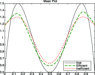
Figure 1: Plot of the mean of the estimated regression curve.

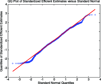
Figure 2: QQ-plot of standardized efficient estimates versus standard normal.

We use a sample of size $250$ and $15$ replications over $200$ evenly spaced grids on $[0,1]$. In this example, approximately $25\%$ of the $200$ observations are censored. Figure 1 displays the average (over replications) of the two estimates. The true regression function chosen possesses a high degree of curvature, with the function increasing less steep to the right of $0.5$ than to the left of $0.5$. Both estimates are capable of capturing the basic structure of the true curve. The efficient estimate appears to adapt better at both peaks and troughs, and the quality of fit declines with the steepness of the true curve. Although it is not shown here, the relative performance of the simple local constant estimator improves toward the feasible oracle estimates when the true regression function has lower degree variation. Figures 2 and 3 are the QQ-plots for the efficient and inefficient estimates, respectively (i.e., $(\hat{g}-E\hat{g})/\mathit{std}(\hat{g}))$. The linear trends in the QQ-plots are distinct with the efficient estimates performing a little better away from the sample means. Figure 4 plots the interquartile range (divided by 1.3) and the standard deviation (across replications) for the efficient estimate against grid points. Performance clearly worsens in the boundary region.

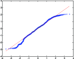
Figure 3: QQ-plot of standardized inefficient estimates versus standard normal.

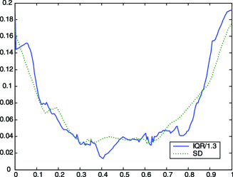
Figure 4: Normalized interquartile range and standard deviation plots for efficient estimates.

Since it is widely perceived that the Silverman’s rule of thumb bandwidth tends to oversmooth, we also performed some experiments with smaller bandwidths. Smaller bandwidth leads to much larger simulation time during optimization, due to higher variance. In terms of goodness of fit, it does not make a big difference with the feasible oracle estimation. However, the improvement of fit for the simple local constant estimation is more pronounced. In that case, the feasible oracle estimation still performs better than the simple estimator, as expected.

Appendix

.1 Local linear estimation

In this section, we first define the local linear marker-dependent estimator, $\hat{\alpha}_{x,L}(y),$ as defined in [30], page 118,

$$\hat{\alpha}_{x,L}(y)=\frac{O_{x,y}^{L}}{E_{x,y}^{L}},$$ (15)

where, with $w=(w_{j})_{j=1}^{d+1}=(x,y)$ and $W_{i}(u)=(W_{ij}(u))_{j=1}^{d+1}=(X_{i},u)$ (to simplify the notation, we consider the same kernel and bandwidth for $x$ and $y$),

$$O_{x,y}^{L} = n^{-1}\sum_{i=1}^{n}\int{K}_{w,b}\{w-W_{i}(u)\}\,\mathrm{d}\overline{N}_{i}(u),\qquad E_{x,y}^{L}=c_{0}-c_{1}^{T}D^{-1}c_{1},$$

$$K_{w,b}(v) = \{K_{b}(v)-K_{b}(v)v^{T}D^{-1}c_{1}\}\qquad(v\in R^{d+1}),$$

$$c_{0} = n^{-1}\sum_{i=1}^{n}\int K_{b}\{w-W_{i}(u)\}C_{i}(u)Z_{i}(u)\,\mathrm{d}u,$$ (16)

$$c_{1j} = n^{-1}\sum_{i=1}^{n}\int K_{b}\{w-W_{i}(u)\}\{w_{j}-W_{ij}(u)\}C_{i}(u)Z_{i}(u)\,\mathrm{d}u,$$

$$d_{jk} = n^{-1}\sum_{i=1}^{n}\int K_{b}\{w-W_{i}(u)\}\{w_{j}-W_{ij}(u)\}\{w_{k}-W_{ik}(u)\}C_{i}(u)Z_{i}(u)\,\mathrm{d}u,$$

and $c_{1}=(c_{1j})_{j=1}^{d+1}$ and $D=(d_{jk})_{j,k=1}^{d+1}$. We then consider the local linear estimator of the integrated conditional hazard function, obtained when we undersmooth in the $y$-direction. First, we define the necessary kernel constants:

$$\overline{K}_{x,b}(v) = \{K_{b}(v)-K_{b}(v)v^{T}\overline{D}^{-1}\overline{c}_{1}\}/(\overline{c}_{0}-\overline{c}_{1}^{T}\overline{D}^{-1}\overline{c}_{1})\qquad(v\in R^{d}),$$

$$\overline{c}_{0} = n^{-1}\sum_{i=1}^{n}K_{b}(x-X_{i}),$$

$$\overline{c}_{1j} = n^{-1}\sum_{i=1}^{n}K_{b}(x-X_{i})(x_{j}-X_{ij}),$$

$$\overline{d}_{jk} = n^{-1}\sum_{i=1}^{n}K_{b}(x-X_{i})(x_{j}-X_{ij})(x_{k}-X_{ik}).$$

We then get that the local linear estimator of the integrated hazard is

$$\widehat{A}_{x,L}(y)=\int_{0}^{y}\frac{\sum_{i=1}^{n}\overline{K}_{x,b}(x-X_{i})}{\sum_{j=1}^{n}\overline{K}_{x,b}(x-X_{j})C_{j}(u)Z_{j}(u)}\,\mathrm{d}\overline{N}_{i}(u).$$

We estimate correspondingly the conditional survival function $S_{x}(y)$ and the regression functions $g_{\mathrm{mn}}^{T}(x)$ and $g_{\mathrm{med}}(x)$ by

$$\widehat{S}_{x,L}(y) = {\prod_{0\leq w\leq y\leq T}}\{1-d\widehat{A}_{x,L}(w)\},$$

$$\hat{g}_{L,\mathrm{mn}}^{T}(x) = -\int_{0}^{T}y\,\mathrm{d}\widehat{S}_{x,L}(y),$$

$$\hat{g}_{L,\mathrm{med}}(x) = \widehat{S}_{x,L}^{-1}(0.5).$$

.2 Proof of results

We restrict attention in the proofs to the case of local constant smoothing (i.e., when $A=C$). The case of local linear smoothing ($A=L$) can be considered in a very similar way and is therefore omitted. Throughout this section, we use the notation $A_{n}\simeq B_{n}$ to indicate that $A_{n}=B_{n}(1+\mathrm{o}_{P}(1))$.

First, we state a useful lemma. Its simple proof is omitted. Let $h(y-)$ be the limit from the left at $y$ for any cadlag function $h$.

Lemma .1

Suppose $A_{1}$ and $A_{2}$ are cadlag functions. Let $S_{1}(y)=\prod_{w\leq y}\{1-\mathrm{d}A_{1}(w)\}$, $S_{2}(y)=\prod_{w\leq y}\{1-\mathrm{d}A_{2}(w)\}$ and

$$Q(y)=\frac{S_{1}(y-)}{S_{2}(y-)}-1\mathit{.}$$

Then

$$\mathrm{d}Q(y)=\frac{S_{1}(y-)}{S_{2}(y-)}\,\mathrm{d}(A_{1}-A_{2})(y).$$

Proof of Theorem 3.1 Define

$$A_{x,C}^{\ast}(y)=\sum_{i=1}^{n}K_{b}(x-X_{i})\int_{0}^{y}\frac{\mathrm{d}\overline{\Lambda}_{i}(u)}{\sum_{j=1}^{n}K_{b}(x-X_{j})C_{j}(u)Z_{j}(u)}.$$

Then

$$\widehat{A}_{x,C}(y)-A_{x}^{\ast}(y)=\sum_{i=1}^{n}K_{b}(x-X_{i})\int_{0}^{y}\frac{\mathrm{d}\overline{M}_{i}(u)}{\sum_{j=1}^{n}K_{b}(x-X_{j})C_{j}(u)Z_{j}(u)}.$$

Let $S_{x}^{\ast}(y)={\prod_{w\leq y}}\{1-\mathrm{d}A_{x}^{\ast}(w)\}.$ We then divide our analysis into an analysis of the variable part

$$V_{x}(y)=\widehat{S}_{x,C}(y)-S_{x}^{\ast}(y)$$ (17)

and of the stable part

$$B_{x}(y)=S_{x}^{\ast}(y)-S_{x}(y).$$ (18)

Note that $V_{x}(y)=S_{x}^{\ast}(y)Q_{x}^{V}(y),$ where $Q_{x}^{V}(y)=\widehat{S}_{x,C}(y)/S_{x}^{\ast}(y)-1,$ $B_{x}(y)=S_{x}(y)Q_{x}^{B}(y)$ and $Q_{x}^{B}(y)=S_{x}^{\ast}(y)/S_{x}(y)-1.$ Using integration by parts, we obtain

$$\hat{g}^{T}_{\mathrm{mn}}(x)-g^{T}_{\mathrm{mn}}(x)=-\int_{0}^{T}y[\widehat{S}_{x,C}(\mathrm{d}y)-S_{x}(\mathrm{d}y)]=\int_{0}^{T}[\widehat{S}_{x,C}(y)-S_{x}(y)]\,\mathrm{d}y=\mathcal{V}(x)+\mathcal{B}(x),$$

where $\mathcal{V}(x)=\int_{0}^{T}V_{x}(y)\,\mathrm{d}y$ and $\mathcal{B}(x)=\int_{0}^{T}B_{x}(y)\,\mathrm{d}y.$ By Lemma .1, we have

$$\mathcal{V}(x) = \int_{0}^{T}S_{x}^{\ast}(y)\int_{0}^{y}\mathrm{d}Q_{x}^{V}(u)\,\mathrm{d}y$$

$$= \int_{0}^{T}S_{x}^{\ast}(y)\int_{0}^{y}\frac{\widehat{S}_{x,C}(u-)}{S_{x}^{\ast}(u-)}\,\mathrm{d}\{\widehat{A}_{x,C}(u)-A_{x,C}^{\ast}(u)\}\,\mathrm{d}y$$

$$= \int_{0}^{T}S_{x}^{\ast}(y)\int_{0}^{y}\frac{\widehat{S}_{x,C}(u-)}{S_{x}^{\ast}(u-)}\sum_{i=1}^{n}K_{b}(x-X_{i})\frac{\mathrm{d}\overline{M}_{i}(u)}{\sum_{j=1}^{n}K_{b}(x-X_{j})C_{j}(u)Z_{j}(u)}\,\mathrm{d}y$$

$$= \sum_{i=1}^{n}\int_{0}^{T}\hat{h}_{x}^{i}(u)\,\mathrm{d}\overline{M}_{i}(u),$$

where

$$\hat{h}_{x}^{i}(u) = \int_{u}^{T}S_{x}^{\ast}(y)\frac{\widehat{S}_{x,C}(u-)}{S_{x}^{\ast}(u-)}K_{b}(x-X_{i})\frac{1}{\sum_{j=1}^{n}K_{b}(x-X_{j})C_{j}(u)Z_{j}(u)}\,\mathrm{d}y$$

$$= \frac{\widehat{S}_{x,C}(u-)}{S_{x}^{\ast}(u-)}\frac{K_{b}(x-X_{i})}{\sum_{j=1}^{n}K_{b}(x-X_{j})C_{j}(u)Z_{j}(u)}\int_{u}^{T}S_{x}^{\ast}(y)\,\mathrm{d}y.\$$

Let

$$\widetilde{\mathcal{V}}(x) = \sum_{i=1}^{n}\int_{0}^{T}h_{x}^{i}(u)\,\mathrm{d}\overline{M}_{i}(u),$$

$$h_{x}^{i}(u) = n^{-1}\frac{K_{b}(x-X_{i})}{\varphi_{x}(u)}\int_{u}^{T}S_{x}(y)\,\mathrm{d}y.$$

Then $\mathcal{V}(x)=\widetilde{\mathcal{V}}(x)+\mathrm{o}_{p}(1)$ and by Nielsen and Linton [31], Proposition 1, $(nb)^{1/2}\widetilde{\mathcal{V}}(x)\Longrightarrow N(0,v(x)),$ where

$$v(x) = p\lim_{n\rightarrow\infty}nb\sum_{i=1}^{n}\int h_{x}^{i}(u)^{2}\,\mathrm{d}\langle\overline{M}_{i}(u)\rangle$$

$$= p\lim_{n\rightarrow\infty}mn^{-1}b\sum_{i=1}^{n}K_{b}(x-X_{i})^{2}\int\frac{1}{\varphi_{x}(u)^{2}}\biggl{\{}\int_{u}^{T}S_{x}(y)\,\mathrm{d}y\biggr{\}}^{2}\alpha_{X_{i}}(u)C_{i}(u)Z_{i}(u)\,\mathrm{d}u$$

$$= \|K\|_{2}^{2}\int\frac{\alpha_{x}(u)}{\varphi_{x}(u)}\biggl{\{}\int_{u}^{T}S_{x}(y)\,\mathrm{d}y\biggr{\}}^{2}\,\mathrm{d}u.$$

The results given in Theorem 3.1 on the variable part follow from standard martingale theory; see, among many others, [31].

We now turn to the bias. Using (D4)–(D6), we have

$$\mathcal{B}(x) = \int_{0}^{T}S_{x}(y)\int_{0}^{y}\mathrm{d}Q_{x}^{B}(u)\,\mathrm{d}y$$

$$= \int_{0}^{T}S_{x}(y)\int_{0}^{y}\frac{{S}_{x}^{\ast}(u-)}{S_{x}(u-)}\,\mathrm{d}\{A_{x}^{\ast}(u)-A_{x}(u)\}\,\mathrm{d}y$$

$$= \int_{0}^{T}S_{x}(y)\int_{0}^{y}\frac{{S}_{x}^{\ast}(u-)}{S_{x}(u-)}\sum_{i=1}^{n}K_{b}(x-X_{i})\frac{C_{i}(u)Z_{i}(u)\{\alpha_{X_{i}}(u)-\alpha_{x}(u)\}\,\mathrm{d}u}{\sum_{j=1}^{n}K_{b}(x-X_{j})C_{j}(u)Z_{j}(u)}\,\mathrm{d}y$$

$$= \frac{1}{2}\mu_{2}(K)b^{2}\int_{0}^{T}S_{x}(y)\int_{0}^{y}\biggl{\{}\frac{\partial^{2}\alpha_{x}(u)}{\partial x^{2}}+\frac{1}{2}\frac{\partial\alpha_{x}(u)}{\partial x}\frac{\partial\varphi_{x}(u)}{\partial x}\biggr{\}}\,\mathrm{d}u\,\mathrm{d}y+\mathrm{o}_{P}(b^{2}).$$

The derivation of the asymptotic theory of the local linear case parallels the local constant case. While the variable part has the same asymptotic distribution, the stable part changes due to the bias properties of the local linear hazard estimator. By checking the derivation of the stable part of the local linear kernel hazard estimation of Nielsen [30], page 119, it is easy to see that the stable part of the local linear estimator can be written as

$$b^{L}(x)=\frac{1}{2}\mu_{2}(K)b^{2}\int_{0}^{T}S_{x}(y)\int_{0}^{y}\frac{\partial^{2}\alpha_{x}(u)}{\partial x^{2}}\,\mathrm{d}u\,\mathrm{d}y.$$

Proof of Theorem 4.1 Consistency of $\widehat{\theta}$ follows from condition (A1) and the fact that

$$\sup_{\theta\in\Theta}|\hat{l}_{\alpha_{0}}(\theta;x)-l(\theta;x)|\stackrel{{\scriptstyle P}}{{\rightarrow}}0$$ (19)

(see, e.g., [40], Theorem 5.7, page 45). The result (19) follows from assumption (A2) and the uniform consistency of $\hat{\alpha}_{x,C}(y);$ this is established in [31], Theorem 2. Actually,

$$\hat{l}_{\alpha_{0}}(\theta;x)-l(\theta;x)$$

$$\quad=\int\biggl{[}\hat{\alpha}_{x,C}(y)-\frac{1}{\theta}\alpha_{0}\biggl{\{}\frac{y}{\theta}\biggr{\}}\biggr{]}^{2}\{\hat{\alpha}_{x,C}(y)\}^{-1}E_{x,y}^{C}w(x,y)\,\mathrm{d}y$$

$$\qquad{}-\int\biggl{[}\alpha_{x}(y)-\frac{1}{\theta}\alpha_{0}\biggl{\{}\frac{y}{\theta}\biggr{\}}\biggr{]}^{2}\{\alpha_{x}(y)\}^{-1}\varphi_{x}(y)w(x,y)\,\mathrm{d}y$$

$$\quad=\int[\hat{\alpha}_{x,C}(y)-\alpha_{x}(y)]^{2}\{\alpha_{x}(y)\}^{-1}\varphi_{x}(y)w(x,y)\,\mathrm{d}y$$

$$\qquad{}+2\int[\hat{\alpha}_{x,C}(y)-\alpha_{x}(y)]\biggl{[}\alpha_{x}(y)-\frac{1}{\theta}\alpha_{0}\biggl{\{}\frac{y}{\theta}\biggr{\}}\biggr{]}\{\alpha_{x}(y)\}^{-1}\varphi_{x}(y)w(x,y)\,\mathrm{d}y$$

$$\qquad{}+\int\biggl{[}\hat{\alpha}_{x,C}(y)-\frac{1}{\theta}\alpha_{0}\biggl{\{}\frac{y}{\theta}\biggr{\}}\biggr{]}^{2}$$

$$\qquad\hphantom{+\int[}{}\times[\{\hat{\alpha}_{x,C}(y)\}^{-1}E_{x,y}^{C}-\{\alpha_{x}(y)\}^{-1}\varphi_{x}(y)]w(x,y)\,\mathrm{d}y$$

and this converges to zero in probability, uniformly in $\theta\in\Theta$.

We next establish asymptotic normality. First, we consider the Taylor expansion

$$0=\hat{l}_{\alpha_{0}}^{\prime}(\widehat{\theta};x)=\hat{l}_{\alpha_{0}}^{\prime}(\theta_{0};x)+\hat{l}_{\alpha_{0}}^{\prime\prime}(\theta^{\ast};x)(\widehat{\theta}-\theta_{0}),$$ (20)

where $\theta^{\ast}$ lies between $\widehat{\theta}$ and $\theta_{0}$. We have

$$\hat{l}_{\alpha_{0}}^{\prime}(\theta;x)=2\int\biggl{[}\hat{\alpha}_{x,C}(y)-\frac{1}{\theta}\alpha_{0}\biggl{\{}\frac{y}{\theta}\biggr{\}}\biggr{]}\rho_{0}\biggl{\{}\frac{y}{\theta}\biggr{\}}\frac{1}{\theta^{2}}\frac{E_{x,y}^{C}}{\hat{\alpha}_{x,C}(y)}w(x,y)\,\mathrm{d}y,$$

where $\rho_{0}(u)=\alpha_{0}(u)+u\alpha_{0}^{\prime}(u)$ and

$$\hat{l}_{\alpha_{0}}^{\prime\prime}(\theta;x) = 2\int\rho_{0}^{2}\biggl{\{}\frac{y}{\theta}\biggr{\}}\frac{1}{\theta^{4}}\frac{E_{x,y}^{C}}{\hat{\alpha}_{x,C}(y)}w(x,y)\,\mathrm{d}y$$

$${}-2\int\biggl{[}\hat{\alpha}_{x,C}(y)-\frac{1}{\theta}\alpha_{0}\biggl{\{}\frac{y}{\theta}\biggr{\}}\biggr{]}\rho_{0}^{\prime}\biggl{\{}\frac{y}{\theta}\biggr{\}}\frac{y}{\theta^{4}}\frac{E_{x,y}^{C}}{\hat{\alpha}_{x,C}(y)}w(x,y)\,\mathrm{d}y$$

$${}-4\int\biggl{[}\hat{\alpha}_{x,C}(y)-\frac{1}{\theta}\alpha_{0}\biggl{\{}\frac{y}{\theta}\biggr{\}}\biggr{]}\rho_{0}\biggl{\{}\frac{y}{\theta}\biggr{\}}\frac{1}{\theta^{3}}\frac{E_{xy}^{C}}{\hat{\alpha}_{x,C}(y)}w(x,y)\,\mathrm{d}y.$$

We first establish the properties of $\hat{l}_{\alpha_{0}}^{\prime}(\theta_{0};x).$ Recall from [31] that

$$\hat{\alpha}_{x,C}(y)-\alpha_{x}(y)=\frac{\mathcal{V}_{x,y}+\mathcal{B}_{x,y}}{E_{x,y}^{C}},$$ (21)

where

$$\mathcal{V}_{x,y} = \frac{1}{n}\sum_{i=1}^{n}\int K_{b}(x-X_{i})k_{h}(y-y^{\prime})\,\mathrm{d}M_{i}(y^{\prime}),$$

$$\mathcal{B}_{x,y} = \frac{1}{n}\sum_{i=1}^{n}\int K_{b}(x-X_{i})k_{h}(y-y^{\prime})[\alpha_{X_{i}}(y^{\prime})-\alpha_{x}(y)]C_{i}(y^{\prime})Z_{i}(y^{\prime})\,\mathrm{d}y^{\prime}.$$

Therefore,

$$\hat{l}_{\alpha_{0}}^{\prime}(\theta_{0};x) = 2\int[\hat{\alpha}_{x,C}(y)-\alpha_{x}(y)]\rho_{0}\biggl{\{}\frac{y}{g(x)}\biggr{\}}\frac{1}{g(x)^{2}}\frac{E_{x,y}^{C}}{\hat{\alpha}_{x,C}(y)}w(x,y)\,\mathrm{d}y$$

$$= 2\int\rho_{0}\biggl{\{}\frac{y}{g(x)}\biggr{\}}\frac{1}{g(x)^{2}}\frac{\mathcal{V}_{x,y}}{\hat{\alpha}_{x,C}(y)}w(x,y)\,\mathrm{d}y$$

$${}+2\int\rho_{0}\biggl{\{}\frac{y}{g(x)}\biggr{\}}\frac{1}{g(x)^{2}}\frac{\mathcal{B}_{x,y}}{\hat{\alpha}_{x,C}(y)}w(x,y)\,\mathrm{d}y$$

$$\simeq 2\int\rho_{0}\biggl{\{}\frac{y}{g(x)}\biggr{\}}\frac{1}{g(x)^{2}}\frac{\mathcal{V}_{x,y}}{\alpha_{x}(y)}w(x,y)\,\mathrm{d}y$$

$${}+2\int\rho_{0}\biggl{\{}\frac{y}{g(x)}\biggr{\}}\frac{1}{g(x)^{2}}\frac{\mathcal{B}_{x,y}}{\alpha_{x}(y)}w(x,y)\,\mathrm{d}y,$$

where the last line follows from [27], Lemma 3. Consider

$$\int\rho_{0}\biggl{\{}\frac{y}{g(x)}\biggr{\}}\frac{1}{g(x)^{2}}\frac{\mathcal{V}_{x,y}}{\alpha_{x}(y)}w(x,y)\,\mathrm{d}y$$

$$\quad=\frac{1}{n}\sum_{i=1}^{n}K_{b}(x-X_{i})\int\biggl{[}\int\rho_{0}\biggl{\{}\frac{y}{g(x)}\biggr{\}}\frac{1}{g(x)^{2}}\frac{1}{\alpha_{x}(y)}k_{h}(y-y^{\prime})w(x,y)\,\mathrm{d}y\biggr{]}\,\mathrm{d}M_{i}(y^{\prime})$$

$$\quad\simeq\sum_{i=1}^{n}\int h_{ni}(x,u)\,\mathrm{d}M_{i}(u),$$

where $h_{ni}(x,u)=n^{-1}K_{b}(x-X_{i})\rho_{0}(u/g(x))w(x,u)/\{g(x)^{2}\alpha_{x}(u)\}.$ By the central limit theorem for martingales, one gets (see, e.g., [31], Proposition 1)

$$\displaystyle(nb)^{1/2}\sum_{i=1}^{n}\int h_{ni}(x,u)\,\mathrm{d}M_{i}(u)\Longrightarrow N(0,\sigma^{2}),$$

$$\displaystyle\sigma^{2}=p\lim_{n\rightarrow\infty}nb\sum_{i=1}^{n}\int h_{ni}^{2}(u)\,\mathrm{d}\langle M_{i}(u)\rangle$$

$$\hskip 20.0pt\displaystyle=p\lim_{n\rightarrow\infty}n^{-1}b\sum_{i=1}^{n}K_{b}^{2}(x-X_{i})\int\frac{\rho_{0}^{2}(u/g(x))}{\alpha_{x}(u)^{2}g(x)^{4}}w(x,u)\alpha_{X_{i}}(u)C_{i}(u)Z_{i}(u)\,\mathrm{d}u$$

$$\displaystyle=\|K\|_{2}^{2}\int\frac{\rho_{0}^{2}(u/g(x))}{\alpha_{x}(u)g(x)^{4}}\varphi_{x}(u)w(x,u)\,\mathrm{d}u.$$

Furthermore,

$$\int\rho_{0}\biggl{\{}\frac{y}{g(x)}\biggr{\}}\frac{1}{g(x)^{2}}\frac{\mathcal{B}_{x,y}}{\alpha_{x}(y)}w(x,y)\,\mathrm{d}y$$

$$\quad=\frac{1}{n}\sum_{i=1}^{n}K_{b}(x-X_{i})\int\!\!\int\rho_{0}\biggl{\{}\frac{y}{g(x)}\biggr{\}}\frac{w(x,y)}{\alpha_{x}(y)g(x)^{2}}k_{h}(y-y^{\prime})$$

$$\hphantom{\quad=\frac{1}{n}\sum_{i=1}^{n}K_{b}(x-X_{i})\int\!\!\int}{}\times[\alpha_{X_{i}}(y^{\prime})-\alpha_{x}(y)]C_{i}(y^{\prime})Z_{i}(y^{\prime})\,\mathrm{d}y^{\prime}\,\mathrm{d}y$$

and it is easily seen that this can be written as a bias term of order $\mathrm{O}(h^{2})+\mathrm{O}(b^{2})$, plus a remainder term of order $\mathrm{o}_{P}((nb)^{-1/2})$.

Finally, note that for any sequence $\delta_{n}\rightarrow 0$, we have

$$\sup_{|\theta-\theta_{0}|\leq\delta_{n}}|\hat{l}_{\alpha_{0}}^{\prime\prime}(\theta;x)-l^{\prime\prime}(\theta_{0};x)|=\mathrm{o}_{P}(1),$$ (22)

where

$$l^{\prime\prime}(\theta_{0};x)=2\int\rho_{0}^{2}\biggl{\{}\frac{u}{g(x)}\biggr{\}}\frac{w(x,u)}{g(x)^{4}}\frac{\varphi_{x}(u)}{\alpha_{x}(u)}\,\mathrm{d}u$$

and $l^{\prime\prime}(\theta_{0};x)>0.$

From (20), we then obtain

$$\hat{g}_{C}^{o}(x)-g(x)=-\{l^{\prime\prime}(\theta_{0};x)\}^{-1}\hat{l}_{\alpha_{0}}^{\prime}(\theta_{0};x)\{1+\mathrm{o}_{P}(1)\}$$

and the asymptotic distribution follows.

Proof of Theorem 4.2 We first consider the infeasible estimator $\hat{\alpha}_{0,A}^{o}(y)$. Consider the following decomposition:

$$\hat{\alpha}_{0,A}^{o}(y) = \frac{\int E^{A}_{x_{,}yg(x)}w(x,yg(x))\,\mathrm{d}x}{\int({E^{A}_{x,yg(x)}w(x,yg(x))}/({g(x)\hat{\alpha}_{x,A}(yg(x))}))\,\mathrm{d}x}$$

$$= \frac{\hat{A}^{o}(y)}{\hat{B}^{o}(y)}$$

$$= \frac{\hat{A}^{o}(y)}{\int{\hat{B}^{o}_{1x}(y)}/{\hat{B}^{o}_{2x}(y)}\,\mathrm{d}x}\qquad\mbox{(say)}$$

$$= \biggl{[}\frac{\hat{A}^{o}(y)}{B^{o}(y)}-\frac{A^{o}(y)}{B^{o}(y)^{2}}\int\frac{\hat{B}_{1x}^{o}(y)}{B_{2x}^{o}(y)}\,\mathrm{d}x+\frac{A^{o}(y)}{B^{o}(y)^{2}}\int\frac{B_{1x}^{o}(y)\hat{B}_{2x}^{o}(y)}{B_{2x}^{o}(y)^{2}}\,\mathrm{d}x\biggr{]}\bigl{(}1+\mathrm{o}_{P}(1)\bigr{)},$$

where $A^{o}(y)=E[(CZ)\{yg(X)\}w\{X,yg(X)\}]$, $B^{o}(y)=E[(CZ)\{yg(X)\}w\{X,yg(X)\}]/\alpha_{0}(y)$, $B^{o}_{1x}(y)=E[(CZ)\{yg(x)\}w\{x,yg(x)\}|X=x]$ and $B^{o}_{2x}(y)=\alpha_{0}(y)$ are the limits of the corresponding quantities with hats.

Straightforward calculations show that

$$\hat{A}^{o}(y) = n^{-1}\sum_{i=1}^{n}(C_{i}Z_{i})\{yg(X_{i})\}w\{X_{i},yg(X_{i})\}+\mathrm{o}_{P}((nh)^{-1/2})+\mathrm{O}(h^{2})+\mathrm{O}(b^{2})$$

and

$$\int\frac{\hat{B}_{1x}^{o}(y)}{B_{2x}^{o}(y)}\,\mathrm{d}x = \alpha_{0}(y)^{-1}n^{-1}\sum_{i=1}^{n}(C_{i}Z_{i})\{yg(X_{i})\}w\{X_{i},yg(X_{i})\}$$

$${}+\mathrm{o}_{P}((nh)^{-1/2})+\mathrm{O}(h^{2})+\mathrm{O}(b^{2}).$$

Next, we consider the term $\int B_{1x}^{o}(y)\hat{B}_{2x}^{o}(y)B_{2x}^{o}(y)^{-2}\,\mathrm{d}x$. Decomposing $\hat{\alpha}_{x,A}(yg(x))=O^{A}_{x,yg(x)}/E^{A}_{x,yg(x)}$ in $\hat{B}_{2x}^{o}(y)$ in a similar way as above, we obtain, after some calculations, that

$$\int\frac{B_{1x}^{o}(y)\hat{B}_{2x}^{o}(y)}{B_{2x}^{o}(y)^{2}}\,\mathrm{d}x$$

$$\quad=B^{o}(y)+\frac{1}{\alpha_{0}(y)}n^{-1}\sum_{i=1}^{n}k_{h}\{yg(X_{i})-Y_{i}\}C_{i}(Y_{i})w(X_{i},yg(X_{i}))$$

$$\qquad{}-\frac{1}{\alpha_{0}(y)}n^{-1}\sum_{i=1}^{n}(C_{i}Z_{i})\{yg(X_{i})\}w\{X_{i},yg(X_{i})\}+\mathrm{o}_{P}((nh)^{-1/2})+\mathrm{O}(h^{2})+\mathrm{O}(b^{2}).$$

Putting the three terms together, we get that

$$\hat{\alpha}_{0,A}^{o}(y) = \frac{1}{B^{o}(y)}n^{-1}\sum_{i=1}^{n}k_{h}\{yg(X_{i})-Y_{i}\}C_{i}(Y_{i})w(X_{i},yg(X_{i}))$$

$${}+\mathrm{o}_{P}((nh)^{-1/2})+\mathrm{O}(h^{2})+\mathrm{O}(b^{2}).$$

We now consider the feasible estimator $\hat{\alpha}_{0,A}(y)$. Write

$$\hat{\alpha}_{0,A}^{o}(y)-E\hat{\alpha}_{0,A}^{o}(y) = \frac{1}{B^{o}(y)}\int k_{h}\{yg(u)-v\}w(u,yg(u))\,\mathrm{d}\bigl{(}\hat{F}^{o}(u,v)-F^{o}(u,v)\bigr{)}$$

$$= \frac{N^{o}(y)}{B^{o}(y)}\qquad\mbox{(say)},$$

where $\hat{F}^{o}(u,v)=n^{-1}\sum_{i=1}^{n}I(X_{i}\leq u,Y_{i}\leq v,C_{i}(Y_{i})=1)$ and $F^{o}(u,v)=E[\hat{F}^{o}(u,v)]$. Therefore,

$$[\hat{\alpha}_{0,A}(y)-E\hat{\alpha}_{0,A}(y)]-[\hat{\alpha}_{0,A}^{o}(y)-E\hat{\alpha}_{0,A}^{o}(y)]$$

(23)

$$\quad=\biggl{[}\frac{1}{B(y)}-\frac{1}{B^{o}(y)}\biggr{]}N(y)+\frac{1}{B^{o}(y)}[N(y)-N^{o}(y)],$$

where $B(y)$ and $N(y)$ are defined by replacing $g(\cdot)$ in the formulas of $B^{o}(y)$ and $N^{o}(y)$ by $\hat{g}(\cdot)$, and where $E\hat{\alpha}_{0,A}(y)$ is the expected value of $\hat{\alpha}_{0,A}(y)$ with $\hat{g}$ considered as fixed. Write

$$N^{o}(y)=h^{-1}\int k(z)w(u,v+hz)\,\mathrm{d}\bigl{(}[\hat{F}^{o}-F^{o}]\bigl{(}u,yg(u)-hz\bigr{)}\bigr{)}.$$

Hence,

$$N(y)-N^{o}(y) = \mathrm{O}\Bigl{(}h^{-1}\sup_{u,|t_{2}-t_{1}|\leq C(nb)^{-1/2}(\log n)^{1/2}}|\hat{F}^{o}(u,t_{1})-F^{o}(u,t_{1})$$

$$\hphantom{\mathrm{O}\Bigl{(}h^{-1}\sup_{u,|t_{2}-t_{1}|\leq C(nb)^{-1/2}(\log n)^{1/2}}|}{}-\hat{F}^{o}(u,t_{2})+F^{o}(u,t_{2})|\Bigr{)}$$

$$= \mathrm{O}_{P}(h^{-1}n^{-1/2}(nb)^{-1/4}(\log n)^{1/4})=\mathrm{o}_{P}((nh)^{-1/2}),$$

provided $nh^{2}b(\log n)^{-1}\rightarrow\infty$. Next, note that $N(y)=\mathrm{O}_{P}((nh)^{-1/2})$, $B(y)-B^{o}(y)=\mathrm{O}_{P}((nb)^{-1/2})=\mathrm{o}_{P}(1)$ and hence (.2) is $\mathrm{o}_{P}((nh)^{-1/2})$. Since it can be easily seen that $E\hat{\alpha}_{0,A}(y)-E\hat{\alpha}_{0,A}^{o}(y)=\mathrm{O}(b^{2})+\mathrm{O}(h^{2})$, it follows that $\hat{\alpha}_{0,A}(y)$ and $\hat{\alpha}_{0,A}^{o}(y)$ are asymptotically equivalent.

Finally, we consider the calculation of the asymptotic variance of $\hat{\alpha}_{0,A}(y)$:

$$\operatorname{AsVar}(\hat{\alpha}_{0,A}(y)) = \frac{n^{-1}}{B^{o}(y)^{2}}\mbox{Var}[k_{h}\{yg(X)-Y\}C(Y)w(X,yg(X))]$$

$$= \frac{n^{-1}}{B^{o}(y)^{2}}\int\!\!\int k_{h}^{2}\{yg(x)-t\}E[C(t)|Y=t,X=x]\,\mathrm{d}F_{x}(t)$$

$$\hphantom{\frac{n^{-1}}{B^{o}(y)^{2}}\int\!\!\int}{}\times w^{2}(x,yg(x))\,\mathrm{d}F(x)\bigl{(}1+\mathrm{o}(1)\bigr{)}$$

$$= \frac{(nh)^{-1}}{B^{o}(y)^{2}}\int k^{2}(u)\,\mathrm{d}uE\{E[C(yg(X))|Y=yg(X),X]$$

$$\hphantom{\frac{(nh)^{-1}}{B^{o}(y)^{2}}\int}{}\times f_{X}(yg(X))w^{2}(X,yg(X))\}\bigl{(}1+\mathrm{o}(1)\bigr{)}.$$

Proof of Theorem 4.3 Consistency of $\widehat{\theta}=\hat{g}^{2-\mathit{step}}(x)$ follows similarly as in the proof of Theorem 4.1 from condition (A1), (19) and the fact that

$$\sup_{\theta\in I_{n}(x)}|\hat{l}_{\hat{\alpha}}(\theta;x)-\hat{l}_{\alpha_{0}}(\theta;x)|\stackrel{{\scriptstyle P}}{{\rightarrow}}0.$$ (24)

Equation (24) follows from assumption (C1) and the uniform consistency of $\hat{\alpha}_{x,C}(y);$ see the proof of Theorem 4.1. For the proof of Theorem 4.3, it remains to show for $\theta_{0}=g(x)$ that for some $\gamma^{*}$,

$$\hat{l}_{\hat{\alpha}}^{\prime}(\theta_{0};x) = \hat{l}_{\alpha_{0}}^{\prime}(\theta_{0};x)+h^{2}\gamma^{*}+\mathrm{o}_{P}((nb)^{-1/2}),$$ (25)

$$\hat{l}_{\hat{\alpha}}^{\prime\prime}(\theta;x) = \hat{l}_{\alpha_{0}}^{\prime\prime}(\theta;x)+\mathrm{o}_{P}(1),$$ (26)

uniformly for $\theta$ in a neighborhood of $\theta_{0}$. Claim (26) follows immediately from assumption (C1). For the proof of (25), note first that

$$\hat{l}_{\hat{\alpha}}^{\prime}(\theta_{0};x)-\hat{l}_{\alpha_{0}}^{\prime}(\theta_{0};x)$$

$$\quad=2\int\biggl{[}\hat{\alpha}_{x,C}(y)-{\frac{1}{\theta_{0}}}\alpha_{0}\biggl{(}{\frac{y}{\theta_{0}}}\biggr{)}\biggr{]}(\widehat{\rho}_{0}-\rho_{0})\biggl{(}\frac{y}{\theta_{0}}\biggr{)}\frac{1}{\theta_{0}^{2}}\frac{E_{x,y}^{C}}{\hat{\alpha}_{x,C}(y)}w(x,y)\,\mathrm{d}y$$

$$\qquad{}+2\int\biggl{[}{\frac{1}{\theta_{0}}}(\hat{\alpha}_{0}-\alpha_{0})\biggl{(}{\frac{y}{\theta_{0}}}\biggr{)}\biggr{]}(\widehat{\rho}_{0}-\rho_{0})\biggl{(}\frac{y}{\theta_{0}}\biggr{)}\frac{1}{\theta_{0}^{2}}\frac{E_{x,y}^{C}}{\hat{\alpha}_{x,C}(y)}w(x,y)\,\mathrm{d}y$$

$$\qquad{}+2\int\biggl{[}{\frac{1}{\theta_{0}}}(\hat{\alpha}_{0}-\alpha_{0})\biggl{(}{\frac{y}{\theta_{0}}}\biggr{)}\biggr{]}\rho_{0}\biggl{(}\frac{y}{\theta_{0}}\biggr{)}\frac{1}{\theta_{0}^{2}}\frac{E_{x,y}^{C}}{\hat{\alpha}_{x,C}(y)}w(x,y)\,\mathrm{d}y,$$

where $\widehat{\rho}_{0}(u)=\hat{\alpha}_{0}(u)+u\hat{\alpha}_{0}^{\prime}(u)$. It follows from (C1) that the second term of the right-hand side is of order $\mathrm{o}_{P}(n^{-2/5})$. From (C1) and (C2), we get that up to a deterministic term of order $\mathrm{O}(h^{2})$, the third term is also of order $\mathrm{o}_{P}(n^{-2/5})$. The first term is equal to $T_{n}+\mathrm{o}_{P}(n^{-2/5})$, where

$$T_{n}=2\int\biggl{[}\hat{\alpha}_{x,C}(y)-{\frac{1}{\theta_{0}}}\alpha_{0}\biggl{(}{\frac{y}{\theta_{0}}}\biggr{)}\biggr{]}(\widehat{\rho}_{0}-\rho_{0})\biggl{(}\frac{y}{\theta_{0}}\biggr{)}\frac{1}{\theta_{0}^{2}}\frac{E_{x,y}^{C}}{{\alpha}_{x}(y)}w(x,y)\,\mathrm{d}y.$$

For the proof of Theorem 4.3, it remains to show that

$$T_{n}=\mathrm{o}_{P}(n^{-2/5}).$$ (27)

By application of (21), we can write $T_{n}=T_{n,1}+T_{n,2}$, where

$$T_{n,1} = 2\int\mathcal{V}_{x,y}(\widehat{\rho}_{0}-\rho_{0})\biggl{(}\frac{y}{\theta_{0}}\biggr{)}\frac{1}{\theta_{0}^{2}}\frac{1}{{\alpha}_{x}(y)}w(x,y)\,\mathrm{d}y,$$

$$T_{n,2} = 2\int\mathcal{B}_{x,y}(\widehat{\rho}_{0}-\rho_{0})\biggl{(}\frac{y}{\theta_{0}}\biggr{)}\frac{1}{\theta_{0}^{2}}\frac{1}{{\alpha}_{x}(y)}w(x,y)\,\mathrm{d}y.$$

It can be easily checked that $T_{n,2}=\mathrm{o}_{P}(n^{-2/5})$ (cf. the proof of Theorem 4.1). The term $T_{n,1}$ can be decomposed into $T_{n,11}+T_{n,12}$, where

$$T_{n,11}=\sum_{i=1}^{n}\int h_{ni}(x,u)\,\mathrm{d}M_{i}(u),\qquad T_{n,12}=\sum_{i=1}^{n}\int g_{ni}(x,u)\,\mathrm{d}M_{i}(u),$$

with

$$h_{ni}(x,u) = \frac{2}{n}K_{b}(x-X_{i})\int\biggl{[}\int(\hat{\alpha}_{0}-\alpha_{0})\biggl{\{}\frac{y}{\theta_{0}}\biggr{\}}\frac{1}{\theta_{0}^{2}}\frac{1}{\alpha_{x}(y)}k_{h}(y-u)w(x,y)\,\mathrm{d}y\biggr{]},$$

$$g_{ni}(x,u) = \frac{2}{n}K_{b}(x-X_{i})\int\biggl{[}\int\biggl{\{}\frac{y}{\theta_{0}}\biggr{\}}(\hat{\alpha}_{0}^{\prime}-\alpha_{0}^{\prime})\biggl{\{}\frac{y}{\theta_{0}}\biggr{\}}\frac{1}{\theta_{0}^{2}}\frac{1}{\alpha_{x}(y)}k_{h}(y-u)w(x,y)\,\mathrm{d}y\biggr{]}.$$

We now show that $T_{n,12}=\mathrm{o}_{P}(n^{-2/5})$. The claim $T_{n,11}=\mathrm{o}_{P}(n^{-2/5})$ can be shown by similar methods. For the proof, we apply [39], Lemma 5.14. This lemma gives a bound on the increments of the empirical process applied to function classes that depend on the sample size. We apply the lemma with a fixed value of $x$, conditional on the event that the number of values of $X_{i}$ in the support of $K_{b}$ is equal to $m$, where $m$ is of the same order as $nb$. We consider the class of functions $g\mathchoice{\nobreak\,\colon}{\nobreak\,\colon}{\nobreak\,\colon\;}{\nobreak\,\colon\;}J(x)\rightarrow\mathbf{R}$ such that, with a sufficiently large constant $C$, for all $z\in J(x)$, $|g(z)-\alpha_{0}^{\prime}(z)|\leq C\delta_{1,n}$ and $|g^{\prime}(z)|\leq C\delta_{2,n}$. We apply the lemma with $\alpha=\beta=1$ and $M=C\delta_{2,n}$. We get that

$$\sup\Biggl{|}\frac{1}{n}\sum_{i=1}^{n}K_{b}(x-X_{i})\int\biggl{[}\int\biggl{(}\frac{y}{\theta_{0}}\biggr{)}g\biggl{(}\frac{y}{\theta_{0}}\biggr{)}\frac{1}{\theta_{0}^{2}}\frac{1}{\alpha_{x}(y)}k_{h}(y-u)w(x,y)\,\mathrm{d}y\biggr{]}\,\mathrm{d}M_{i}(u)\Biggr{|}$$

is of order $\mathrm{O}_{P}(\delta_{1,n}^{1/2}\delta_{2,n}^{1/2}(nb)^{-1/2}+\delta_{2,n}(nb)^{-1})=\mathrm{o}_{P}((nb)^{-1/2})$. This shows that $T_{n,12}=\mathrm{o}_{P}(n^{-2/5})$ and thus concludes the proof of Theorem 4.3.

References

- [1] Andersen, P.K., Borgan, O., Gill, R.D. and Keiding, N. (1988). Censoring, truncation and filtering in statistical models based on counting process theory. Contemp. Math. 80 19–59. MR0999006
- [2] Andersen, P.K., Borgan, O., Gill, R.D. and Keiding, N. (1992). Statistical Models Based on Counting Processes. New York: Springer. MR1198884
- [3] Beran, R. (1981). Nonparametric regression with randomly censored survival data. Technical report, Department of Statistics, University of California, Berkeley.
- [4] Berkson, J. (1980). Minimum chi-square, not maximum likelihood. Ann. Statist. 8 457–487. MR0568715
- [5] Buchinsky, M. and Hahn, J. (1998). An alternative estimator for the censored quantile regression model. Econometrica 66 653–671. MR1627038
- [6] Buckley, J. and James, I. (1979). Linear regression with censored data. Biometrika 66 429–436.
- [7] Dabrowska, D.M. (1987). Non-parametric regression with censored survival time data. Scand. J. Statist. 14 181–192. MR0932943
- [8] Dabrowska, D.M. (1992). Nonparametric quantile regression with censored data. Sankhyā Ser. A 54 252–259. MR1192099
- [9] Duncan, G.M. (1986). A semi-parametric censored regression estimator. J. Econometrics 32 5–24. MR0853043
- [10] Efron, B. and Johnstone, I.M. (1990). Fisher’s information in terms of the hazard rate. Ann. Statist. 18 38–62. MR1041385
- [11] Fan, J. and Gijbels, I. (1994). Censored regression: Local linear approximations and their applications. J. Amer. Statist. Assoc. 89 560–570. MR1294083
- [12] Fan, J. and Gijbels, I. (1996). Local Polynomial Regression. London: Chapman and Hall. MR1383587
- [13] Fernandez, L. (1986). Non-parametric maximum likelihood estimation of censored regression models. J. Econometrics 32 35–57. MR0853044
- [14] Fleming, T.R. and Harrington, D.P. (1991). Counting Processes and Survival Analysis. New York: Wiley. MR1100924
- [15] Heckman, J.J. (1976). The common structure of statistical models of truncation, sample selection, and limited dependent variables and a simple estimator for such models. Ann. Econ. Social Measurement 15 475–492.
- [16] Heuchenne, C. and Van Keilegom, I. (2007a). Nonlinear regression with censored data. Technometrics 49 34–44. MR2345450
- [17] Heuchenne, C. and Van Keilegom, I. (2007b). Location estimation in nonparametric regression with censored data. J. Multivariate Anal. 98 1558–1582. MR2370107
- [18] Heuchenne, C. and Van Keilegom, I. (2010). Estimation in nonparametric location-scale regression models with censored data. Ann. Inst. Statist. Math. 62 439–464.
- [19] Honoré, B.E. and Powell, J.L. (1994). Pairwise difference estimators of censored and truncated regression models. J. Econometrics 64 241–278. MR1310525
- [20] Horowitz, J.L. (1986). A distribution free least squares estimator for censored linear regression models. J. Econometrics 32 59–84. MR0853045
- [21] Horowitz, J.L. (1988). Semiparametric M-estimation of censored linear regression models. Adv. Econometrics 7 45–83.
- [22] Johansen, S. and Gill, R.D. (1990). A survey of product-integration with a view toward application in survival analysis. Ann. Statist. 18 1501–1555. MR1074422
- [23] Koul, H., Susarla, V. and Van Ryzin, J. (1981). Regression analysis with randomly right censored data. Ann. Statist. 42 1276–1288. MR0630110
- [24] Lewbel, A. and Linton, O.B. (2002). Nonparametric censored and truncated regression. Econometrica 70 765–779. MR1913830
- [25] Linton, O.B. (1997). Efficient estimation of additive nonparametric regression models. Biometrika 84 469–474. MR1467061
- [26] Linton, O.B. (2000). Efficient estimation of generalized additive nonparametric regression models. Econom. Theory 16 502–523. MR1790289
- [27] Linton, O.B., Nielsen, J.P. and Van de Geer, S. (2003). Estimating multiplicative and additive hazard functions by kernel methods. Ann. Statist. 31 464–492. MR1983538
- [28] Linton, O.B and Xiao, Z. (2002). A nonparametric regression estimator that adapts to error distribution of unknown form. Econom. Theory 23 371–413. MR2359245
- [29] Mammen, E. and Nielsen, J.P. (2007). A general approach to the predictability issue in survival analysis with applications. Biometrika 94 873–892. MR2416797
- [30] Nielsen, J.P. (1998). Marker dependent kernel hazard estimation from local linear estimation. Scand. Actuar. J. 2 113–124. MR1659309
- [31] Nielsen, J.P. and Linton, O.B. (1995). Kernel estimation in a marker dependent hazard model. Ann. Statist. 23 1735–1748. MR1370305
- [32] Powell, J.L. (1984). Least absolute deviations estimation for the censored regression model. J. Econometrics 25 303–325. MR0752444
- [33] Powell, J.L. (1986a). Symmetrically trimmed least squares estimation for Tobit models. Econometrica 54 1435–1460. MR0868151
- [34] Powell, J.L. (1986b). Censored regression quantiles. J. Econometrics 32 143–155. MR0853049
- [35] Rebolledo, R. (1980). Central limit theorems for local martingales. Z. Wahrsch. Verw. Gebiete 51 269–286. MR0566321
- [36] Ritov, Y. (1990). Estimation in a linear regression model with censored data. Ann. Statist. 18 27–41. MR1041395
- [37] Stone, C.J. (1977). Consistent nonparametric regression. Ann. Statist. 5 595–645. MR0443204
- [38] Tibshirani, R. (1984). Local likelihood estimation. Ph.D. thesis, Stanford University.
- [39] Van de Geer, S. (2000). Empirical Processes in M-Estimation. Cambridge: Cambridge Univ. Press.
- [40] Van der Vaart, A.W. (1998). Asymptotic Statistics. Cambridge: Cambridge Univ. Press. MR1652247
- [41] Van Keilegom, I. and Akritas, M.G. (1999). Transfer of tail information in censored regression models. Ann. Statist. 27 1745–1784. MR1742508
- [42] Van Keilegom, I. and Veraverbeke, N. (1998). Bootstrapping quantiles in a fixed design regression model with censored data. J. Statist. Planning Inference 69 115–131. MR1631161