A weak lensing analysis of the Abell 383 cluster.

Abstract

Aims. In this paper we use deep CFHT and SUBARU $uBVRIz$ archival images of the Abell 383 cluster (z=0.187) to estimate its mass by weak lensing.

Methods. To this end, we first use simulated images to check the accuracy provided by our KSB pipeline. Such simulations include both the STEP 1 and 2 simulations, and more realistic simulations of the distortion of galaxy shapes by a cluster with a Navarro-Frenk-White (NFW) profile. From such simulations we estimate the effect of noise on shear measurement and derive the correction terms. The $R-$band image is used to derive the mass by fitting the observed tangential shear profile with a NFW mass profile. Photometric redshifts are computed from the $uBVRIz$ catalogs. Different methods for the foreground/background galaxy selection are implemented, namely selection by magnitude, color and photometric redshifts, and results are compared. In particular, we developed a semi-automatic algorithm to select the foreground galaxies in the color-color diagram, based on observed colors.

Results. Using color selection or photometric redshifts improves the correction of dilution from foreground galaxies: this leads to higher signals in the inner parts of the cluster. We obtain a cluster mass $M_{\rm vir}=7.5^{+2.7}_{-1.9}\times 10^{14}$ $M_{\odot}$: such value is $\sim$ 20% higher than previous estimates, and is more consistent the mass expected from X–ray data. The $R$-band luminosity function of the cluster is finally computed, giving a total luminosity $L_{\rm tot}=(2.14\pm 0.5)$ $\times$ $10^{12}\leavevmode\nobreak\ L_{\odot}$ and a mass to luminosity ratio $M/L\sim 300M_{\odot}/L_{\odot}$.

1 Introduction

Weak gravitational lensing is a unique technique that allows to probe the distribution of dark matter in the Universe. It measures the very small distortions in the shapes of faint background galaxies, due to foreground mass structures. This technique requires a very accurate measurement of the shape parameters as well as the removal of the systematic effects affecting them. In addition, galaxies to be used in the weak lensing analysis must be carefully selected so that they do not include a significant fraction of unlensed sources, with redshift smaller than that of the lens. This would introduce a dilution and therefore an underestimated signal, in particular towards the cluster center (see Broadhurst et al. 2005): such effect may be the reason of the under-prediction by weak lensing of the observed Einstein radius, by a factor of $\sim 2.5$ (Smith et al. 2001; Bardeau et al. 2005). The optimal case would happen if photometric redshifts were available. Even if for weak lensing high accuracy in their estimate are not required for individual galaxies, on average we need at least $\sigma_{z}/(1+z)<0.1$: this implies having observations in several bands, spanning a good wavelength range. If few bands are available, an uncontaminated background sample can be obtained by selecting only galaxies redder than the cluster red sequence (Broadhurst et al. 2005). However, such method often does not allow to get a number density of background sources high enough to allow an accurate weak lensing measure. Including galaxies bluer than the red sequence (Okabe et al. 2010) requires a careful selection of the color offset, as bluer galaxies can be still contaminated by late–types members of the cluster. Finally, if more than two bands are available, Medezinski et al. (2010) discussed how to identify cluster members and the foreground population as overdensities in the color-color space.

In this paper we exploit deep $uBVRIz$ images of the cluster Abell 383, taken with the MEGACAM and SUPRIME camera mounted on the 3.6m CFHT and 8m SUBARU telescopes respectively, and publicly available. The mass of the cluster is derived by weak lensing, and values obtained by different selection methods are compared. The properties of the cluster are reviewed in Sect.2. Data reduction is discussed in Sect.3. In Sect. 4 we describe the algorithm used for the shape measurement, and some improvements for the removal of biases. The accuracy in the mass estimate is derived by comparison with simulations. In Sect. 5, we first summarize the different methods for the selection of the background galaxies from which the lensing signal is measured. Such methods are applied to the case of Abell 383, and the masses derived in such way are then compared. Finally, in Sect. 6 we compare the mass derived in this paper with literature values, both by X–rays and weak lensing; a comparison is also done with the mass expected for the $R$–band luminosity, derived from the luminosity function of Abell 383.

A standard cosmology was adopted in this paper: $\Omega_{\Lambda}=0.7$, $\Omega_{M}=0.3$, $H_{0}=70$ km s^-1 Mpc^-1, giving a scale of 2.92 kpc/arcsec at the redshift of Abell 383.

2 Abell 383

Abell 383 is an apparently well relaxed cluster of galaxies of richness class 2 and of Bautz-Morgan type II-III (Abell et al. 1989), located at z = 0.187 (Fetisova et al. 1993). It is dominated by the central cD galaxy, a blue-core emission-line Bright Cluster Galaxy (BCG), that is aligned with the X-ray peak Smith et al. (2001). Abell 383 is one of the clusters of the XBACs sample (X-ray-Brightest Abell-type Clusters), observed in the ROSAT All-Sky Survey (RASS; Voges 1992): its X-ray luminosity is $8.03\times 10^{44}$ erg sec^-1 in the 0.1-2.4 keV band and its X-ray temperature is 7.5 keV (Ebeling et al. 1996). A small core radius, a steep surface brightness profile and an inverted deprojected temperature profile, show evidence of the presence of a cooling flow, as supported by the strong emission lines in the optical spectra of its BCG (Rizza et al. 1998).

An extensive study of this cluster was carried out by Smith et al. (2001), in which lensing and X-ray properties were analyzed on deep optical HST images and ROSAT HRI data, respectively. A complex system of strong lensed features (a giant arc, two radial arcs in the center and numerous arclets) were identified in its HST images, some of which are also visible in the deep SUBARU data used here.

3 Data retrieval and reduction

The cluster Abell 383 was observed with the SUPRIME camera mounted at the 8m SUBARU telescope: SUPRIME is a ten CCDs mosaic, with a $34\times 27$ arcmin² field of view (Miyazaki et al. 2002). Data are publicly available in the $BVRIz$ filters, with total exposure times of 7800s ($R$), $\sim$ 6000s ($B$, $V$), 3600s ($I$) and 1500s ($z$); they were retrieved using the SMOKA Science Archive facility. Data were collected from seven different runs, amounting to $\sim 55$GB. Details about the observation nights and exposure times for each band are given in Table 1. The data reduction was done using the VST–Tube imaging pipeline, specifically developed for the VLT Survey Telescope (VST, Capaccioli et al. 2005) but adaptable to other existing or future multi-CCD cameras (Grado et al. 2011) .

The field of Abell 383 was also observed in the $u^{*}$ band with the MEGACAM camera attached on the Canada-France Hawaii Telescope (CFHT), with a total exposure time of 10541s. The preprocessed images were retrieved from the CADC archive.

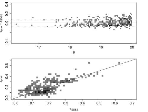
Figure 1: Density plots comparing the photometric redshifts in the Abell 383 field available from the SDSS, and those here computed from the $uBVRIz$ photometry.

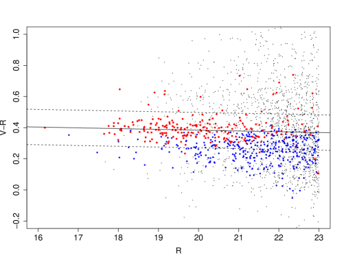
Figure 2: $V-R$ vs $R$ color plot: red and blue points are galaxies at $z_{\rm phot}=0.187\pm$ 0.1 and classified as early and late-type, respectively; dashed lines shows the $\pm 1\sigma$ levels.

The basic reduction steps were performed for each frame, namely overscan correction, flat fielding, correction of the geometric distortion due to the optics, and sky background subtraction. It is worth mentioning that to improve the photometric accuracy, a sky superflat was used.

Table 1: Summary of observations done with the MEGACAM ($u$) and SUPRIME ($BVRIz$) cameras, used in this paper.

Date	Band	Exp. Time	Total
23 Dec 2003	$u^{*}$	8381s
21 Jan 2004	$u^{*}$	2160s
			10541s
09 Sept 2002	$B$	2400s
08 Jan 2008	$B$	2400s
09 Jan 2008	$B$	1200s
			6000s
02 Oct 2002	$V$	4320s
01 Oct 2005	$V$	1800s
			6120s
12 Nov 2007	$R_{c}$	2400s
08 Jan 2008	$R_{c}$	5400s
			7800s
02 Oct 2002	$I_{c}$	3600s
			3600s
10 Sept 2002	$z^{\prime}$	1500s
			1500s

Geometric distortions were first removed from each exposure, using the Scamp tool and taking the USNO-B1 as the astrometric reference catalog. The internal accuracy provided by Scamp, as measured by positions of the same sources in different exposures, is $\sim 0.05$ arcsec. Different exposures were then stacked together using SWarp. The coaddition was done in such a way that all the images had the same scale and size.

The photometric calibration of the $BVRI$ bands was performed using the standard Stetson fields, observed in the same nights of the data. In the case of the $z$ band, we used a pointing also covered by the Stripe 82 scans in the Sloan Digital Sky Survey (SDSS); the SDSS photometry of sources identified as point-like was used to derive the zero point in the SUBARU image.

In the case of the MEGACAM-CFHT $u^{*}$ band images, reduced images and photometric zero points are already available from the CADC public archive, hence only astrometric calibration and stacking were required.

Table 2 summarizes the photometric properties of the final coadded images (average FWHMs and limiting magnitudes for point-like sources) for each band. All magnitudes were converted to the AB system; magnitudes of sources classified as galaxies were corrected for Galactic extinction using the Schlegel maps (Schlegel et al. 1998).

The weak lensing analysis was done on the $R-$band image. The masking of reflection haloes and diffraction spikes near bright stars are performed by ExAM, a code developed for this purpose. In short, ExAM takes the SExtractor catalog as input, locates the stellar locus in the size-magnitude diagram (see Sect. 4.1), picks out stars with spike-like features from the isophotal shape analysis, and outputs mask region file that may be visualized in the DS9 software, and finally creates a mask image in FITS format. The reflection haloes are masked by estimating the background contrast near the bright stars, whose positions are obtained from the USNO–B1. The effective area available after removal of regions masked in such way was 801 arcmin². Catalogs for the other bands were extracted using SExtractor in dual–mode, where the $R-$band image was used as the detection image.

Table 2: Photometric properties of the coadded images; FWHM (arcsec) and limiting magnitudes (in the AB system) were computed for point-like sources. The signal to noise (SNR) is defined as SNR=FLUX_AUTO/FLUXERR_AUTO.

Band	FWHM	mag (SNR=5)	mag (SNR=10)
$u^{*}$	1.3	26.1	25.3
$B$	0.99	27.0	26.2
$V$	0.95	26.6	25.7
$R_{c}$	0.82	27.1	26.1
$I_{c}$	0.97	25.0	24.2
$z^{\prime}$	0.74	24.7	23.9

Photometric redshifts were computed from $uBVRIz$ photometry, using the ZEBRA code (Feldmann et al. 2006). This software allows to define 6 basic templates (elliptical, Sbc, Sbd, irregular and two starburst SEDs), and to compute log-interpolations between each pair of adjacent templates. We first applied to the $BVz$ magnitudes the offset derived within the COSMOS survey by Capak et al. (2007), that is +0.19 ($B$), +0.04 ($V$), -0.04 ($z$). We then convolved the stellar spectra from the Pickles’ library (Pickles 1985) with the transmission curves used for each filter, and derived the offsets for the other filters, that is: 0.0 ($u$), 0.0 ($R$), +0.05 ($I$). Fig. 3 shows the comparison of the model colors with those derived for the stars in our catalogs, after the above offsets were applied. We also verified that the offsets derived in this way are consistent with those obtained by running ZEBRA in the so-called photometry-check mode, that allows to compute magnitude offsets minimizing the average residuals of observed versus template magnitudes.

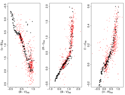
Figure 3: Observed (red dots) and model colors (black dots) for stars, after the offsets given in the text were applied. Model colors were derived convolving the Pickles’ library of stellar spectra with the filter transmission curves.

Figure 4: Distribution of the photometric redshifts computed from the $uBVRIz$ data for $R<25$ mag.

We then removed from the catalog those galaxies with a photometric redshift $z_{\rm ph}>3$ and $\sigma_{z}/(1+z)>0.1$, where $\sigma_{z}$ was derived from the 68%–level errors computed in ZEBRA. The distribution of the so-obtained photometric redshifts is displayed in Fig. 4. The accuracy of the so obtained photometric redshifts was derived from the comparison with the SDSS photometric redshifts of galaxies in the SDSS (DR7), whose rms error is $\sim 0.025$ for $r^{\prime}<20$ mag. We derived (Fig. 1) a systematic offset $\Delta z/(1+z)=0.003$ and an rms error $\sigma\Delta z/(1+z)=0.07$. As a further check, we extracted from our catalog those galaxies classified by ZEBRA as early-type, with $R<23$ mag and $|z_{\rm phot}-0.187|=0.1$. As expected, such galaxies define a red sequence (Fig.2): this was fitted as $V-R=a+bR$, with $a=0.5$, $b=-6\times 10^{-3}$.

4 Shape measurement

Ellipticities of galaxies were estimated using the KSB approach (Luppino & Kaiser 1997): even if such algorithm does not allow to achieve accurate measurements of very low shear signals, $\gamma\lesssim 10^{-3}$, it is nevertheless adequate in the case of weak lensing by clusters, as discussed e.g. by Gill et al. (2009) and Romano et al. (2010).

In our KSB implementation, the SExtractor software was modified to compute all the relevant quantities, namely the raw ellipticity $e$, the smear polarizability $P^{\rm sm}$, and the shear polarizability $P^{\rm sh}$. The centers of detected sources were measured using the windowed centroids in SExtractor.

The KSB approach assumes that the PSF can be described as the sum of an isotropic component (simulating the effect of seeing) and an anisotropic part. The correction of the observed ellipticity $e_{\rm obs}$ for the anisotropic part is computed as:

$$e_{\rm aniso}=e_{\rm obs}-P^{\rm sm}p,$$ (1)

where (starred terms indicate that they are derived from measurement of stars):

$$p=e^{*}_{\rm obs}/P^{\rm sm*}.$$ (2)

The intrinsic ellipticity $e$ of a galaxy, and the reduced shear, $g=\gamma/(1-\kappa)$, are then related by:

$$e_{\rm aniso}=e+P^{\gamma}g$$ (3)

The term $P^{\gamma}$, introduced by Luppino & Kaiser (1997) as the pre–seeing shear polarizability, describes the effect of seeing and is defined to be:

$$P^{\gamma}=P^{\rm sh}-P^{\rm sm}\frac{P^{\rm sh*}}{P^{\rm sm*}}\equiv P^{\rm sh}-P^{\rm sm}q.$$ (4)

The final output of the pipeline is the quantity $e_{\rm iso}=e_{\rm aniso}/P^{\gamma}$, from which the average reduced shear, $\left\langle g\right\rangle=\left\langle e_{\rm iso}\right\rangle$, provided that the average intrinsic ellipticity vanishes, $\left\langle e\right\rangle=0$.

The ellipticity calculation is done by using a window function in order to suppress the outer, noisy part of a galaxy: the function is usually chosen to be Gaussian with size $\theta$. The size of the window function is commonly taken as the radius containing 50% of the total flux of the galaxy (as given by e.g. the FLUX_RADIUS parameter in SExtractor). In our case, we proceed as follows. We define a set of bins with $\theta$ varying between 2 and 10 pixels (sources with smaller and larger sizes are rejected in our analysis), and a step of 0.5 pixel. For each bin we compute $e_{\rm obs}$, $P^{\rm sh}$ and $P^{\rm sm}$, and the ellipticity signal to noise ratio defined by Eq. 16 in Erben et al. (2001):

$${\rm SNe}(\theta)=\frac{\int I(\theta)W(|\theta|)d^{2}\theta}{\sigma_{\rm sky}\sqrt{\int W^{2}(|\theta|)d^{2}\theta}}.$$ (5)

The optimal size of the window function, $\theta_{\rm max}$, is then defined as the value that maximizes SNe. Fig.5 shows the typical trend of SNe, which was normalized for display purposes, as a function of $\theta$. It can be seen (Fig.  6) that, on average, there is a constant offset between $\theta_{\rm max}$ and FLUX_RADIUS. Below SNe $\sim$ 5, FLUX_RADIUS starts to decrease: this provides an estimate of limit on SNe, below which the shape measurement is not meaningful any more.

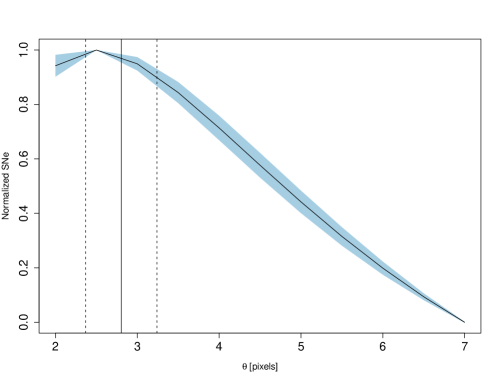
Figure 5: SNe is displayed as a function of the window function size, $\theta$, used to measure ellipticities. For display purposes, galaxies were selected to have the same value of $\theta_{\rm max}$, and SNe was normalized so that min(SNe)=0, max(SNe)=1. The vertical lines indicate the average (solid) and standard deviation (dashed) of FLUX_RADIUS for the same galaxies.

Figure 6: Running median of FLUX_RADIUS-$\theta_{\rm max}$ as a function of SNe. The vertical line shows the limit chosen for the selection of background galaxies.

The terms $p$ and $q$, derived from stars, must be evaluated at each galaxy position: this is usually done fitting them by a polynomial (see e.g. Radovich et al. 2008), whose order must be chosen to fit the observed trend, without overfitting. The usage of the window function introduces a calibration factor, which is compensated by the $P^{\gamma}$ term. This implies that stellar terms must be computed and fitted with the same value of $\theta$ used for each galaxy (Hoekstra et al. 1998). An alternative approach, not based on a constant (and somehow arbitrary) order polynomial, is given e.g. by Generalized Additive Models: we found that the implementation in R (function GAM in the mgcv library) provides good results. Fig. 7 shows fitting and residuals of the anisotropic PSF component: from the comparison between the results obtained with polynomial and GAM fitting we see that in the latter case we obtain lower residuals, in particular in the borders of the image. To quantify the improvement compared to the usage of the polynomial, we obtain $\left\langle e_{\rm aniso,1}\right\rangle=(1\pm 5)\times 10^{-4}$, $\left\langle e_{\rm aniso,2}\right\rangle=(-2\pm 9)\times 10^{-4}$ with a polynomial of order 3, $\left\langle e_{\rm aniso,1}\right\rangle=(2\pm 4)\times 10^{-4}$, $\left\langle e_{\rm aniso,2}\right\rangle=(1\pm 7)\times 10^{-4}$ with the GAM algorithm. The values of the fitted terms $p$ and $q$ at the positions of the galaxies are predicted by GAM, that also provides an estimate of the standard errors of the predictions, $\Delta p$ and $\Delta q$. From error propagation, the uncertainty on $e_{\rm iso}$ was computed as:

$$\Delta e_{\rm iso}^{2}=(\Delta e_{\rm aniso}/P^{\gamma})^{2}+(e_{\rm aniso}(P^{\gamma})^{-2}\Delta P^{\gamma})^{2},$$ (6)

where $(\Delta e_{\rm aniso})^{2}=(\Delta e_{\rm obs})^{2}+(P^{\rm sm}\Delta p)^{2}$ and $(\Delta P^{\gamma})^{2}=(P^{\rm sm}\Delta q)^{2}$; uncertainties on the measured values of $P^{\rm sm}$ and $P^{\rm sh}$ were not considered.

For each galaxy, a weight is defined as:

$$w=\frac{1}{\Delta{e_{0}}^{2}+\Delta e_{\rm iso}^{2}},$$ (7)

where $\Delta{e_{0}}\sim 0.3$ is the typical intrinsic rms of galaxy ellipticities.

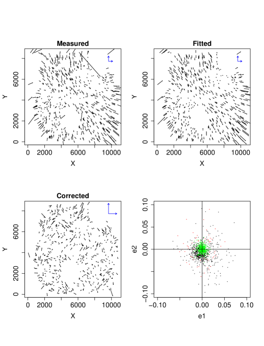
Figure 7: PSF anisotropy correction derived with the GAM algorithm: the first three panels show the ellipticity pattern (measured, fitted and residuals; X and Y are in pixels). The scale is displayed by the arrows in the upper right part of each panel ($e=0.05$). In the next panel, black dots are the measured values, green dots are after the correction; values rejected during fitting are marked in red. The last row shows for comparison the corrected ellipticities obtained using for the fit a polynomial of order 3.

4.1 Star-galaxy classification

Stars and galaxies were separated in the magnitude (MAG_AUTO) vs. size plot. Instead of using e.g. FLUX_RADIUS as the estimator of size, we used the quantity $\delta$=MU_MAX-MAG_AUTO, where MU_MAX is the peak surface brightness above background. Saturated stars were found in the locus of sources with constant MU_MAX; in the $\delta$ vs. MAG_AUTO plot, stars are identified as sources in the vertical branch. Sources with $\delta$ lower than stars were classified as spurious detections. In addition, we rejected those sources for which $\delta$ is $\sim 2\sigma$ larger than the median value. This is to exclude from the sample of stars used to compute the PSF correction terms, those sources for which the shape measurement may be wrong due to close blended sources, noise, etc.

We further excluded those galaxies with $w<1$ or SNe $<5$, for which the ellipticity measurement is not meaningful.

4.2 Error estimate in shear and mass measurement

In the case of faint galaxies used for the weak lensing analysis, the ellipticity is underestimated due to noise. Such effect is not included in the $P^{\gamma}$ term, which can be only computed on stars with high signal to noise ratio. Schrabback et al. (2010) proposed the following parametrization for such bias, as a function of the signal to noise:

$$m=\frac{e_{k}-e_{m}}{e_{m}}=a*({\rm SNe})^{b},$$ (8)

where $e_{m}$ and $e_{k}$ are the ellipticities before and after the correction respectively. Such parameters were derived using the STEP1 (Heymans et al. 2006) and STEP2 (Massey et al. 2007) simulations, where both PSF and shear are constant for each simulated image. We obtain $a=-0.1$ and $b=-0.45$, which corresponds to a bias $m$ changing from $\sim 5\%$ for SNe =5 to $<2\%$ for SNe $>50$. After such correction was applied, we computed again the average shear from the STEP1 and STEP2 simulations, and obtained a typical bias of $\sim$ 3% for SNe $=$ 5.

We then estimated the accuracy on the mass that can be obtained from an image with the same noise and depth as in the $R-$band SUBARU image. To this end we dropped the assumption on constant shear, and produced more realistic simulations: the effect on galaxy shapes by weak lensing from a galaxy cluster was produced using the SHUFF code, that will be described in a separate paper (Huang et al., in preparation). To summarize, the code takes as input a catalog of galaxies produced by the Stuff tool; it computes the shear produced by a standard mass profile (e.g. Navarro-Frenk-White, NFW hereafter) and applies it to the ellipticities of the galaxies behind the cluster. Such catalog is then used in the SkyMaker software, configured with the telescope parameters suitable for the SUBARU telescope and with the exposure time of the $R-$band image, producing a simulated image; the background rms of such image was set to be as close as possible to that of the real image. We considered for the lens a range of masses at $\log M_{\rm vir}/M_{\odot}=13.5,14,14.5,15.0$, and a NFW mass profile with $c_{\rm vir}=6$. Each simulation was repeated 50 times for each mass value, randomly changing the morphology, position and redshift of the galaxies.

For each of these images, we run our lensing pipeline with the same configuration used for the real data. The density of background galaxies used for the lensing analysis was $\sim 20$ gals arcmin^-2. The fit of the mass was done as described in Radovich et al. (2008) and Romano et al. (2010): the expressions for the radial dependence of tangential shear $\gamma_{T}$ derived by Bartelmann (1996) and Wright & Brainerd (2000) were used, and the NFW parameters ($M_{\rm vir}$, $c_{\rm vir}$) were derived using a maximum likelihood approach. In addition, the 2D projected mass can be derived in a non-parametric way by aperture densitometry, where the mass profile of the cluster is computed by the $\zeta$ statistics (Fahlman et al. 1994; Clowe et al. 1998):

$$\zeta(\theta_{1})=\bar{\kappa}(\theta\leq\theta_{1})-\bar{\kappa}(\theta_{2}<\theta\leq\theta_{\rm out})=2\int^{\theta_{2}}_{\theta_{1}}\left\langle\gamma_{T}\right\rangle d\ln\theta$$ (9)

$$+\frac{2}{1-(\theta_{2}/\theta_{\rm out})^{2}}\int^{\theta_{\rm out}}_{\theta_{2}}\left\langle\gamma_{T}\right\rangle d\ln\theta.$$

The mass is estimated as $M_{\rm ap}(\theta_{1})=\pi\theta_{1}^{2}\zeta(\theta_{1})\Sigma_{\rm crit}$, and $\theta_{\rm out}$ is chosen so that $\bar{\kappa}(\theta_{2},\theta_{\rm out})\sim 0$.

The average errors on mass estimate obtained in such way are displayed in Table  3, showing that masses can be estimated within an uncertainty of $<$ 20% for $M\geq 10^{14}M_{\odot}$. Such accuracy only includes the contribute due to shape measurement and mass fitting method, but it does not include the uncertainty due to the selection of the lensed galaxies.

Finally, the masses derived by aperture densitometry are $\sim$ 1.3 higher than those obtained by mass fitting: this is in agreement with Okabe et al. (2010), who find $M_{\rm 2D}/M_{\rm 3D}=1.34$ for virial overdensity.

Table 3: Masses derived by simulations with NFW model fitting ($M_{\rm 3D}$) and aperture densitometry ($M_{\rm 2D}$). Input masses used for each simulation are given in the first column ($M_{\rm in}$).

$M_{\rm in}$	$M_{\rm 3D}$	$M_{\rm 2D}/M_{\rm 3D}$
$10^{14}M_{\odot}$	$10^{14}M_{\odot}$
0.316	$0.31\pm 0.13$	$1.3\pm 0.9$
1.00	$1.01\pm 0.24$	$1.4\pm 0.4$
3.16	$3.12\pm 0.36$	$1.4\pm 0.3$
10.0	$10.1\pm 0.5$	$1.3\pm 0.1$

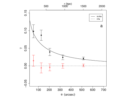
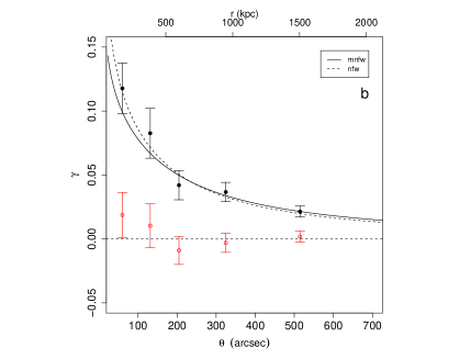
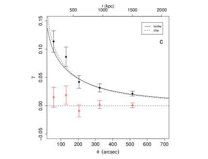
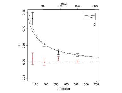
Figure 8: Shear profiles obtained with the different selection methods (see Table 4, where the parameters derived for each model are given). The fitting was done using the maximum likelihood approach. Binned points are shown for display purposes only. In panel a, the curves obtained by the two models (nfw/mnfw) overlap.

5 Results

One of the most critical source of systematic errors, which can lead to an underestimation of the true WL signal, is dilution of the distortion due to the contamination of the background galaxy catalog by unlensed foreground and cluster member galaxies (see e.g. Broadhurst et al. 2005). The dilution effect increases as the cluster-centric distance decreases because the number density of cluster galaxies that contaminate the faint galaxy catalog is expected to roughly follow the underlying density profile of the cluster. Thus, correcting for the dilution effect is important to obtain unbiased, accurate constraints on the cluster parameters and mass profile.

As discussed by Broadhurst et al. (2005); Okabe et al. (2010); Oguri et al. (2010), the selection of background galaxies to be used for the weak lensing analysis can be done taking those galaxies redder than the cluster red sequence. However, such selection produces a low number density (10 galaxies/arcmin² in our case), and correspondingly high uncertainties in the derived parameters. In the following, we compare the results obtained by different methods. We first assumed that no information on the redshift is available, and that photometry from only one band is available (magnitude cut), or from more than two bands (color selection). Finally, we included in our analysis the photometric redshifts. The density of background galaxies is $\sim$ 25-30 galaxies/arcmin², see Table 4.

In order to derive the mass, we need to know the critical surface density:

$$\Sigma_{\rm crit}=\frac{c^{2}}{4\pi G}\frac{D_{s}}{D_{l}D_{ls}}=\frac{c^{2}}{4\pi G}\frac{1}{D_{l}\beta},$$ (10)

$D_{ls}$, $D_{s}$, and $D_{l}$ being the angular distances between lens and source, observer and source, and observer and lens respectively. This quantity should be computed for each lensed galaxy. As the reliability of photometric redshifts for the faint background galaxies is not well known, we prefer to adopt the single sheet approximation, where all background galaxies are assumed to lie at the same redshift, defined as $\beta(z_{s})=\left\langle\beta(z)\right\rangle$. In the case of the selection based only on magnitude or colors, such value was derived from the COSMOS catalog of photometric redshifts (Capak et al. 2007), to which the same cuts used for the Abell 383 catalog are applied. Later on, we computed $\beta(z_{s})$ from the photometric redshifts themselves, and compared such two values.

The mass was computed both by fitting a NFW profile ($M_{\rm 3D}=M_{\rm vir}$), and by aperture densitometry ($M_{\rm 2D}$). In the case of the NFW fit, in addition to a 2-parameters fit (virial mass $M_{\rm vir}$ and concentration $c_{\rm vir}$), we also show (MNFW) the results obtained using the relation proposed by Bullock et al. (2001) between $M_{\rm vir}$, $c_{\rm vir}$ and the cluster redshift $z_{\rm cl}$:

$$c_{\rm vir}=\frac{K}{1+z_{\rm cl}}\left(\frac{M_{\rm vir}}{M_{\star}}\right)^{\alpha},$$ (11)

with $M_{\star}=1.5\times 10^{13}/h$ $M_{\odot}$, $K=9$, $\alpha=-0.13$.

The shear profiles obtained from the different methods discussed below are displayed in Fig. 8; also displayed are the average values of tangential and radial components of shear, computed in bins selected to contain at least 200 galaxies, and centered on the BCG: this is also where the peak of the X–ray emission is located (Rizza et al. 1998). In order to check the possible error introduced by a wrong center, we considered a grid around the position of the BCG, with a step of 2 arcsec: for each position in the grid, we took it as the center, performed the fit and derived the mass. Within 30 arcsec, we obtain that the rms is $\sigma(M_{\rm vir})<5\%$. The NFW parameters obtained by model fitting, and the reduced $\chi^{2}$ computed from the binned average tangential shear, are given in Table 4.

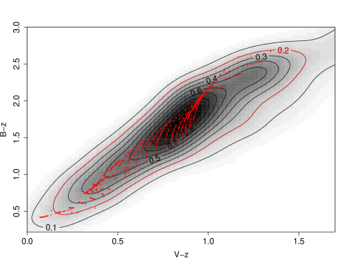
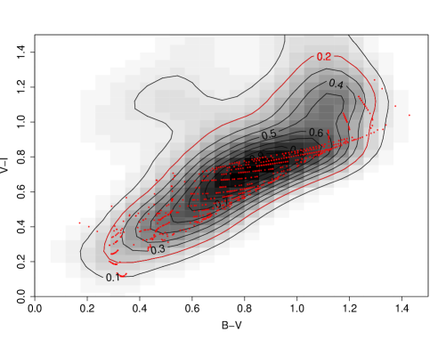
Figure 9: Color selection of foreground galaxies ($z_{\rm phot}<0.2$). The contour in red is the density level chosen for the selection; the points display the model colors computed by ZEBRA for this redshift range.

The magnitude cut is the simplest approach as it only requires photometry from the same band in which the lensing measurement is done. Taking galaxies in the range 23 $<$ $R$ $<$ 26 mag (a), produces a sample dominated by faint background galaxies, but the inner regions of the cluster may still present an unknown contamination by cluster galaxies.

To improve the selection, we proceeded as follows. The locus of foreground galaxies was first found, allowing a better separation of different galaxy populations (see Medezinski et al. 2010, and references therein), compared e.g. to methods based on the selection of only red galaxies. Here we considered two colors selections, namely $B-z$ vs. $V-z$ (b) and $B-V$ vs. $V-I$ (c), with $21<R<26$ mag. For intermediate redshifts ($z\sim 0.2$), foreground and background objects are well separated in such two colors diagrams. We explored the possibility to find the best selection criteria based only on the observed colors, without any information on the redshift of the galaxies. To this end, we developed a semi-automatic procedure, implemented in the R language (R Development Core Team 2010). We first selected bright ($R<$ 21 mag) galaxies, which are expected to be mainly at $z_{\rm ph}<0.2$. A kernel density estimate, obtained by the kde2d package in R (Venables & Ripley 2002) was then applied to these points, giving the plots displayed in Fig.9: the normalization was done so that the value of the maximum density in the binned data was equal to one. The boundary of the foreground galaxy region was then defined by the points within the same density level $l$ (e.g., $l=0.2$). Such region was converted to a polygon using the splancs package in R, that also allows to select for a given catalog those sources whose colors lie inside or outside the polygon. A comparison with the model colors obtained in ZEBRA from the convolution of the spectral templates with filter transmission curves, shows that colors inside the area selected in such way are consistent with those expected for galaxies at redshift $<$ 0.2. Galaxies classified as foreground in such way were therefore excluded from the weak lensing analysis.

We finally used photometric redshifts (d), both for the selection of background galaxies, defined as those with $21<R<26$ mag, $0.3<z_{\rm ph}<3$, and to compute the average value of $\beta$: we obtain in such way $\beta(z_{s})=0.74$, in good agreement with the value obtained from the COSMOS catalog with the same magnitude and redshift selection, $\beta(z_{s})=0.73$.

The effect of the different selections on the residual presence of cluster galaxies is displayed in Fig. 11, showing the density of background galaxies computed in different annuli around the cluster: a clear increase of the density in the inner regions is visible in case a, which indicates that magnitude selection alone does not allow to completely remove the contamination by cluster galaxies. Such contamination is greatly reduced by color selection, and the optimal result is given by photometric redshifts, as expected. As a further check, we also found for each method that the tangential shear signals of the rejected ’foreground/cluster’ galaxies average out. In the following discussion, we take as reference the results from case d, which is very close to c in terms of uncertainties on fitted parameters, density of background galaxies and residuals in the radial component of the shear.

It was pointed out in Hoekstra (2003) and Hoekstra et al. (2010) that large-scale structures along the line of sight provide a source of uncertainty on cluster masses derived by weak lensing, which is usually ignored and increases as a larger radius ($\theta_{\rm max}$) is used in the fitting. The uncertainty introduced by such component on the mass estimate can be $\sim$ 10-20% for a cluster with $M=10^{15}M_{\odot}$ at $z\sim 0.2$, $\theta_{\rm max}=10$ arcmin as in our case (see Fig. 6 and 7 in Hoekstra (2003)), which is comparable to the uncertainties derived in the fitting.

Table 4: Best-fit NFW parameters: for each selection method, in the upper row both $M_{\rm vir}$ and $c_{\rm vir}$ were taken as free parameters, in the lower row the ($M_{\rm vir}$, $c_{\rm vir}$, $z_{\rm cl}$) relation (Bullock et al. 2001) was used. The reduced $\chi^{2}$ was computed from the binned values displayed in Fig. 8. Also given are the values of $M_{\rm 200}$: the larger uncertainties are due to the fact they were derived from the fitted values ($M_{\rm vir},c_{\rm vir}$). The values of $M_{\rm 2D}$ before and after applying the factor 1.34 (Sect.4.2) are displayed in the upper and lower rows, respectively.

Method	$M_{\rm vir}$	$c_{\rm vir}$	$r_{\rm vir}$	$M_{\rm 200}$	$\chi^{2}$/d.o.f.	$M_{\rm 2D}$	Density
	$10^{14}M_{\odot}$		arcsec	$10^{14}M_{\odot}$		$10^{14}M_{\odot}$	gal/arcmin2
a	$7.78_{-2.21}^{3.34}$	$4.73_{-1.49}^{1.99}$	$698_{-73}^{88}$	$6.44^{7.94}_{-3.23}$	1.13	12.3 $\pm$ 2.98	30
	$7.80_{-1.52}^{1.65}$	$4.71_{-0.12}^{0.13}$	$699_{-49}^{46}$	$6.46_{-1.68}^{1.98}$	1.13	9.20 $\pm$ 2.22
b	$7.61_{-2.04}^{2.94}$	$5.77_{-1.69}^{2.33}$	$693_{-69}^{80}$	$6.42^{6.85}_{-3.21}$	0.40	8.14 $\pm$ 3.15	25
	$9.00_{-1.69}^{1.85}$	$4.62_{-0.11}^{0.13}$	$733_{-49}^{47}$	$7.44_{-1.86}^{2.20}$	0.70	6.07 $\pm$ 2.35
c	$7.51_{-2.00}^{2.90}$	$5.40_{-1.52}^{2.13}$	$690_{-68}^{79}$	$6.30^{6.15}_{-3.08}$	0.87	10.5 $\pm$ 3.03	28
	$8.38_{-1.57}^{1.69}$	$4.67_{-0.11}^{0.13}$	$716_{-48}^{45}$	$6.94_{-1.73}^{2.01}$	0.61	7.82 $\pm$ 2.26
d	$7.54_{-1.91}^{2.66}$	$5.68_{-1.60}^{2.11}$	$691.05_{-64}^{73}$	$6.35^{6.45}_{-3.02}$	1.1	10.2 $\pm$ 2.94	25
	$8.73_{-1.60}^{1.75}$	$4.64_{-0.11}^{0.12}$	$725.77_{-47}^{46}$	$7.22_{-1.77}^{2.09}$	1.90	7.59 $\pm$ 2.19

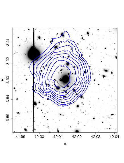
Figure 10: Weak lensing S-map showing the mass distribution derived by weak lensing; overlaid is the central region of the Abell 383 field.

Also displayed in Table 4 are the projected masses computed by aperture densitometry from Eq. 4.2, at a distance from the cluster center $r=r_{\rm vir}$, and $\theta_{2}=900\arcsec$, $\theta_{\rm out}=1000\arcsec$. A good agreement is found between these masses and the values computed from parametric fits, if we take into account the expected ratio $M_{\rm 2D}/M_{\rm 3D}=1.34$ (see Sect. 4.2).

From the catalog based on photometric redshifts selection (case d), we finally derived the S-map introduced by Schirmer et al. (2004), that is: $S=M_{\rm ap}/\sigma_{M_{\rm ap}}$, where

$$M_{\rm ap} = \frac{\sum_{i}e_{t,i}w_{i}Q(|\theta_{i}-\theta_{0}|)}{\sum_{i}{w_{i}}}$$ (12)

$$\sigma^{2}_{M_{\rm ap}} = \frac{\sum_{i}e^{2}_{i}w^{2}_{i}Q^{2}(|\theta_{i}-\theta_{0}|)}{2(\sum_{i}{w_{i}})^{2}},$$

The map was obtained by defining a grid of points along the image; the tangential components $e_{t,i}$ of the lensed galaxy ellipticities were computed taking as center each point in such grid. The weight $w_{i}$ was defined in Eq. 7, and $Q$ is a Gaussian function as in Radovich et al. (2008):

$$Q(|\theta-\theta_{0}|)=\frac{1}{\pi\theta^{2}_{s}}\exp\left(-\frac{(\theta-\theta_{0})^{2}}{\theta^{2}_{s}}\right),$$ (13)

where $\theta_{0}$ and $\theta_{s}$ are the center and size of the aperture ($\theta_{s}\sim 1.5$ arcmin). The S-map is displayed in Fig. 10, showing a quite circular mass distribution centered on the BCG.

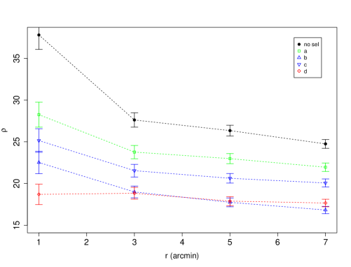
Figure 11: Density (gal/arcmin²) of background galaxies used for the lensing analysis, as a function of the distance from the cluster, for the different selection methods here considered. The case with no selection is also displayed for comparison.

Table 5: Luminosity function parameters, and uncertainties. $\Phi_{\star}$ is in units of deg^-2.

	Best-fit	Standard error
$\alpha$	-1.06	0.07
$m_{\star}$	18.32	0.39
$\Phi_{\star}/10^{3}$	1.273	0.374

6 Discussion

Several mass measurements of this cluster are available in literature, based on different data and/or methods. Schmidt & Allen (2007) used Chandra data and modeled the dark matter halo by a generalized NFW profile, obtaining a mass value $M_{\rm vir}=9.16^{+1.89}_{-1.85}\times 10^{14}M_{\odot}$ and a concentration value $c_{\rm vir}=5.08^{+0.55}_{-1.03}$.

A weak lensing analysis of Abell 383 was done by Bardeau et al. (2007) using CFH12K data in the $B$, $R$, $I$ filters. For the shape measurements they used a Bayesian method implemented into the IM2SHAPE software. To retrieve the weak lensing signal they selected the background galaxies as those within $21.6<R<24.9$ mag and ($R-I$)$\gtrsim 0.7$, obtaining a number density of $\sim 10$ gal arcmin^-2. Their fit of the shear profile by a NFW profile gave as result a mass of $M_{200}=4.19\pm 1.46\times h^{-1}_{70}10^{14}M_{\odot}$ at $r_{200}=1.32\pm 0.17h^{-1}_{70}$ Mpc and a concentration value of $c=2.62\pm 0.69$.

Another weak lensing mass estimate of Abell 383 from CHF12K data was obtained by Hoekstra (2007) using two bands, $B$ (7200 s) and $R$ (4800 s). The background sample was selected by a magnitude cut $21<R<24.5$, from which cluster red sequence galaxies were discarded. The remaining contamination was estimated from the stacking of several clusters by assuming that fraction of cluster galaxies $f_{gc}$ was a function of radius $\propto r^{-1}$. This function was used to correct the tangential shear measurements. As discussed in Okabe et al. (2010), this kind of calibration method does not allow to perform an unbiased cluster-by-cluster correction. Assuming a NFW profile, the fitted virial mass of Abell 383 was $M_{\rm vir}=2.8^{1.6}_{-1.5}\times h^{-1}10^{14}M_{\odot}$.

Abell 383 belongs to the clusters sample selected for the Local Cluster Substructure Survey (LoCuSS) project (P.I. G. Smith). Within this project, a weak lensing analysis of this cluster has been recently performed by Okabe et al. (2010) using SUBARU data in two filters, $i^{\prime}$ (36 minutes) and $V$ (30 minutes). In addition to a magnitude cut $22<i<26$ mag, they used the color information to select galaxies redder and bluer than the cluster red sequence. Looking at the trend of the lensing signal as function of the color offset, they selected the sample where the dilution were minimized, obtaining a background sample of $\sim 34$ gal arcmin^-2 for the computation of tangential shear profile of the cluster. The fit of this profile by a NFW model did not give an acceptable fit: the virial mass computed assuming a NFW profile was $M_{\rm vir}=3.62^{+1.15}_{-0.86}\times h^{-1}10^{14}M_{\odot}$ with a high concentration parameter $c_{\rm vir}=8.87^{+5.22}_{-3.05}$. The same authors also derived the projected mass, obtaining $M_{2D}=8.69\times h^{-1}10^{14}M_{\odot}$ at the virial radius.

Scaling such mass values to $h=0.7$, we derive $M_{\rm vir}\sim(4-5)\times 10^{14}$ $M_{\odot}$. This value is still consistent within uncertainties with the value derived in the present analysis ($M_{\rm vir}=(7.5^{2.7}_{-1.9}\times 10^{14}$ $M_{\odot}$, $c_{\rm vir}=5.7^{2.1}_{-1.6}$, case d). In our case, we obtain however a better agreement with both the values of $M_{\rm vir}$ and $c_{\rm vir}$ given by the X-ray data, and a better consistency between parametric and non-parametric mass estimates, once the projection factor is taken into account. This may be due either to how the selection of background/foreground galaxies was done, or to a higher accuracy in the shape measurement as a combination of the deeper image and calibration of the bias due to SNR (Sect. 4).

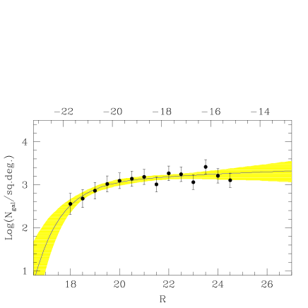
Figure 12: $R$-band LF of the galaxies in Abell 383. Data points are derived by binning the data in magnitude bins of 0.5 mag and error bars by Poissonian errors; the curve traces the best-fitting LF and the shaded area marks the model uncertainty, obtained by a bootstrap technique.

Finally, we computed the luminosity function (LF hereafter) in the $R$-band and derived the total luminosity by integrating the fitted Schechter (Schechter 1976) function as described in Radovich et al. (2008). In order to obtain the cluster LF, that is the number of galaxies per unit luminosity and volume belonging to the cluster, we need to remove from our catalog all the background and foreground galaxies. Usually, this is done by statistically subtracting the galaxy counts in a control field from galaxy counts in the cluster direction. Here we take advantage of the selection on the color-color diagrams described in Sect. 5, and extract a catalog that includes cluster, foreground and residual background galaxies. The last two components were further removed by the statistical subtraction, where we defined as cluster area the circular region around the cluster center of radius r=10.2 arcmin (1.3Mpc); the control field was instead defined as the area outside the circle of radius r=15.3 arcmin. For the best-fitting procedure to the Schechter function, we adopted conventional routines of minimization on the binned distributions. Best-fitting parameters are listed in Table 5. The $R$-band total luminosity, calculated as the Schechter integral, is $L_{\rm tot}=(2.14\pm 0.5)$ $\times$ $10^{12}\leavevmode\nobreak\ L_{\odot}$. The errors were estimated by the propagation of the $68\%$-confidence-errors of each parameter.

For comparison, we then used the relation in Popesso et al. (2007) between $M_{\rm 200}$ and the optical luminosity, $L_{\rm op}$, to see whether the mass obtained in this paper is consistent with the value expected for that luminosity. According to this relation, the mass expected for such luminosity is $M_{\rm 200}=(4.73\pm 1.3)\times$ $10^{14}\leavevmode\nobreak\ M_{\odot}$, in good agreement with the value derived by our weak lensing analysis, $M_{\rm 200}\sim 6.3\times$ $10^{14}\leavevmode\nobreak\ M_{\odot}$ (case d), corresponding to $M/L\sim 300M_{\odot}/L_{\odot}$.

7 Conclusions

We have computed the cluster Abell 383 mass by weak lensing, using a deep $R$-band image taken with the Suprime camera on the Subaru telescope. Catalogs extracted from combined CFHT+SUBARU $uBVRIz$ images were used to derive photometric redshifts, and improve the weak lensing analysis. The data were reduced using a pipeline developed in–house, that was specifically designed for wide-field imaging data. The ellipticities, from which the shear signal was derived, were measured using a pipeline based on the KSB approach. We discussed some aspects that may improve the results, namely the size of the window used to suppress the noise from the outer part of the galaxies, the selection of a limit on SNR below which the measurement ellipticity is not accurate enough, and a weighting scheme where uncertainties on spatial fitting of the PSF correction terms were taken into account.

The accuracy on the mass estimate by weak lensing available with our KSB pipeline was first derived on simulated images which were built in such a way to mimic as closely as possible the background noise and the depth of the real image. From these simulations we conclude that the mass can be measured with an uncertainty $\sim$ 5-10% for $\log M/M_{\odot}\geq 14.5$. Such accuracy takes into account the measurement errors of the ellipticity, but not the errors due to e.g. the foreground/background galaxy separation, that may introduce an underestimate of the mass. The impact of such selection was evaluated by comparing three methods for the foreground/background galaxy separation, namely: magnitude cut in one band, color selection and usage of photometric redshifts. All methods gave consistent estimates of the total virial mass, but from the shear profile it can be seen that a dilution of the signal in the inner regions is still present, in the case of a simple magnitude cut. Color selection and photometric redshifts provide better results, even if the accuracy of the photometric redshifts is not high due to the few available bands. The virial mass of Abell 383 here obtained by NFW model fitting is in agreement with the value obtained from the non-parametric mass estimate, that is $M_{\rm vir}\sim 7\times 10^{14}$ $M_{\odot}$. Other previous weak lensing analyses give $M_{\rm vir}\sim(4-5)\times 10^{14}$ $M_{\odot}$: the value found in this paper seems more in agreement with the value found by X-ray data, and we also have a better agreement between parametric and non-parametric estimates, compared to e.g. Okabe et al. (2010).

Finally, we estimated the $R$-band LF of Abell 383, and derived the total $R$-band luminosity of the cluster: starting from this value and using the relation between mass and luminosity found for clusters by Popesso et al. (2007), we conclude that the mass derived by weak lensing is consistent with the value expected for this luminosity.

8 Acknowledgments

L.F., Z.H. and M.R. acknowledge the support of the European Commission Programme 6-th framework, Marie Curie Training and Research Network “DUEL”, contract number MRTN-CT-2006-036133. L.F. was partly supported by the Chinese National Science Foundation Nos. 10878003 & 10778725, 973 Program No. 2007CB 815402, Shanghai Science Foundations and Leading Academic Discipline Project of Shanghai Normal University (DZL805), and Chen Guang project with No. 10CG46 of Shanghai Municipal Education Commission and Shanghai Education Development Foundation. A.R. acknowledges support from the Italian Space Agency (ASI) contract Euclid-IC I/031/10/0. We are grateful to the referee for the useful comments that improved this paper.

References

- Abell et al. (1989) Abell, G. O., Corwin, Jr., H. G., & Olowin, R. P. 1989, ApJS, 70, 1
- Bardeau et al. (2005) Bardeau, S., Kneib, J., Czoske, O., et al. 2005, A&A, 434, 433
- Bardeau et al. (2007) Bardeau, S., Soucail, G., Kneib, J., et al. 2007, A&A, 470, 449
- Bartelmann (1996) Bartelmann, M. 1996, A&A, 313, 697
- Broadhurst et al. (2005) Broadhurst, T., Takada, M., Umetsu, K., et al. 2005, ApJ, 619, L143
- Bullock et al. (2001) Bullock, J. S., Kolatt, T. S., Sigad, Y., et al. 2001, MNRAS, 321, 559
- Capaccioli et al. (2005) Capaccioli, M., Mancini, D., & Sedmak, G. 2005, The Messenger, 120, 10
- Capak et al. (2007) Capak, P., Aussel, H., Ajiki, M., et al. 2007, ApJS, 172, 99
- Clowe et al. (1998) Clowe, D., Luppino, G. A., Kaiser, N., Henry, J. P., & Gioia, I. M. 1998, ApJ, 497L, 61
- Ebeling et al. (1996) Ebeling, H., Voges, W., Bohringer, H., et al. 1996, MNRAS, 281, 799
- Erben et al. (2001) Erben, T., Waerbeke, L. V., Bertin, E., Mellier, Y., & Schneider, P. 2001, A&A, 366, 717
- Fahlman et al. (1994) Fahlman, G., Kaiser, N., Squires, G., & Woods, D. 1994, ApJ, 437, 56
- Feldmann et al. (2006) Feldmann, R., Carollo, C. M., Porciani, C., et al. 2006, MNRAS, 372, 565
- Fetisova et al. (1993) Fetisova, T. S., Kuznetsov, D. Y., Lipovetskij, V. A., Starobinskij, A. A., & Olowin, R. P. 1993, Astronomy Letters, 19, 198
- Gill et al. (2009) Gill, M. S. S., Young, J. C., Draskovic, J. P., et al. 2009, ArXiv:0909.3856
- Grado et al. (2011) Grado, A., Capaccioli, M., Limatola, L., & Getman, F. 2011, ArXiv:1102.1588
- Heymans et al. (2006) Heymans, C., Van Waerbeke, L., Bacon, D., et al. 2006, MNRAS, 368, 1323
- Hoekstra (2003) Hoekstra, H. 2003, MNRAS, 339, 1155
- Hoekstra (2007) Hoekstra, H. 2007, MNRAS, 379, 317
- Hoekstra et al. (1998) Hoekstra, H., Franx, M., Kuijken, K., & Squires, G. 1998, ApJ, 504, 636
- Hoekstra et al. (2010) Hoekstra, H., Hartlap, J., Hilbert, S., & van Uitert, E. 2010, ArXiv:1011.1084
- Luppino & Kaiser (1997) Luppino, G. & Kaiser, N. 1997, ApJ, 475, 20
- Massey et al. (2007) Massey, R., Heymans, C., Bergé, J., et al. 2007, MNRAS, 376, 13
- Medezinski et al. (2010) Medezinski, E., Broadhurst, T., Umetsu, K., et al. 2010, MNRAS, 405, 257
- Miyazaki et al. (2002) Miyazaki, S., Komiyama, Y., Sekiguchi, M., et al. 2002, PASJ, 54, 833
- Oguri et al. (2010) Oguri, M., Takada, M., Okabe, N., & Smith, G. P. 2010, MNRAS, 405, 2215
- Okabe et al. (2010) Okabe, N., Takada, M., Umetsu, K., Futamase, T., & Smith, G. P. 2010, PASJ, 62, 811
- Pickles (1985) Pickles, A. J. 1985, ApJS, 59, 33
- Popesso et al. (2007) Popesso, P., Biviano, A., Böringher, H., & Romaniello, M. 2007, A&A, 464, 451
- R Development Core Team (2010) R Development Core Team. 2010, R: A Language and Environment for Statistical Computing, R Foundation for Statistical Computing, Vienna, Austria, ISBN 3-900051-07-0
- Radovich et al. (2008) Radovich, M., Puddu, E., Romano, A., Grado, A., & Getman, F. 2008, A&A, 487, 55
- Rizza et al. (1998) Rizza, E., Burns, J. O., Ledlow, M. J., et al. 1998, MNRAS, 301, 328
- Romano et al. (2010) Romano, A., Fu, L., Giordano, F., et al. 2010, A&A, 514, A88+
- Schechter (1976) Schechter, P. 1976, ApJ, 203, 297
- Schirmer et al. (2004) Schirmer, M., Erben, T., Schneider, P., Wolf, C., & Meisenheimer, K. 2004, A&A, 420, 75
- Schlegel et al. (1998) Schlegel, D. J., Finkbeiner, D. P., & Davis, M. 1998, ApJ, 500, 525
- Schmidt & Allen (2007) Schmidt, R. W. & Allen, S. W. 2007, MNRAS, 379, 209
- Schrabback et al. (2010) Schrabback, T., Hartlap, J., Joachimi, B., et al. 2010, A&A, 516, 63
- Smith et al. (2001) Smith, G. P., Kneib, J., Ebeling, H., Czoske, O., & Smail, I. 2001, ApJ, 552, 493
- Venables & Ripley (2002) Venables, W. N. & Ripley, B. D. 2002, Modern Applied Statistics with S, 4th edn. (New York: Springer), isbn 0-387-95457-0
- Voges (1992) Voges, W. 1992, in European Southern Observatory Conference and Workshop Proceedings, Vol. 43, European Southern Observatory Conference and Workshop Proceedings, ed. A. Heck & F. Murtagh, 139–+
- Wright & Brainerd (2000) Wright, C. O. & Brainerd, T. G. 2000, ApJ, 534, 34