Chiral symmetry restoration and deconfinement in strong magnetic fields

Abstract:

I review recent results obtained within chiral effective models, on the phase structure of hot quark matter in a strong magnetic background. After a brief introduction, I focus on the results obtained within two chiral models improved with the Polyakov loop. The models differ for the content of interactions, but both of them are tuned to reproduce Lattice QCD thermodynamics at zero and imaginary chemical potential. One of them takes into account an explicit Polyakov loop dependence of the coupling; the other one neglects this contribution, but takes into account multi-quark interactions. A comparison between the phase diagrams of the two models is presented.

1 Introduction

The study of the influence of external factors on the vacuum of Quantum Chromodynamics (QCD), is one of the most attractive topics of modern physics. Thanks to Lattice QCD simulations, it is established that at vanishing quark chemical potential, two crossovers take place in a narrow range of temperature; one for quark deconfinement, and another one for the (approximate) restoration of chiral symmetry [1, 2, 3, 4, 5]. Besides, powerful analytic and semi-analytic techniques have been developed to understand the coupling between chiral symmetry restoration and deconfinement, see [6] and references therein.

An alternative approach to the physics of strong interactions, which is capable to capture some of the non-perturbative properties of the QCD vacuum, is the Nambu-Jona Lasinio (NJL) model [7], see Refs. [8] for reviews. In this model, the QCD gluon-mediated interactions are replaced by effective interactions among quarks, which are built in order to respect the global symmetries of QCD. The NJL model has been improved recently [9, 10], in order to be capable to compute quantities which are related to the confinement-deconfinement transition of QCD. In pure glue theory, color confinement can be characterized by the expectation value of the Polyakov loop [11], which is an order parameter for the center symmetry of the color gauge group. In theories with dynamical fermions, the Polyakov loop is still a good indicator for the confinement-deconfinement transition, as suggested by Lattice data at zero chemical potential [1, 2, 3, 4, 5]. Motivated by this property, the Polyakov extended Nambu-Jona Lasinio model (P-NJL model) has been introduced [9, 10], in which the concept of statistical confinement replaces that of the true confinement of QCD, and an effective potential describing interaction among the chiral condensate and the Polyakov loop is achieved by the coupling of quarks to a background temporal gluon field, then integrating over quark fields in the functional integral representation of the partition function. Chiral models with the Polyakov loop have been studied extensively in many contexts [12, 13, 14, 15, 16, 17, 18, 19, 20, 21].

In this talk, I report on results obtained in Refs. [22, 23, 24], about deconfinement and chiral symmetry restoration of hot quark matter in a strong magnetic background. Related Lattice studies can be found in [25, 26]; previous studies of QCD and of QCD-like theories in a magnetic background can be found in [27, 28, 29, 30]. Strong magnetic fields might be produced in non-central heavy ion collisions [31, 32]. For example, at the center-of-mass energy reachable at LHC, $\sqrt{s_{NN}}\approx 4.5$ TeV, the magnetic field can be as large as  $eB\approx 15m_{\pi}^{2}$ according to [32]. It has been argued that in these conditions, the sphaleron transitions of finite temperature QCD, give rise to Chiral Magnetic Effect [31, 33, 34]. This adds a phenomenological interest to the study presented here, beside the purely theoretical one aforementioned.

The plan of the talk is as follow: after a brief introduction to the model used in calculations, I discuss the results about Polyakov loop expectation value and chiral condensate in a magnetic background. Then, I collect these results in the form of a phase diagram in the temperature-magnetic field strength plane. Finally, I discuss briefly about improved results that take into account a tree-level coupling among the chiral condensate and the Polyakov loop, and show within the model how this coupling modifies the response of hot quark matter to a magnetic background.

2 The model: propagator and one-loop thermodynamic potential

I consider a model in which quark matter is described by the following lagrangian density:

$${\cal L}=\bar{\psi}\left(i\gamma^{\mu}D_{\mu}-m\right)\psi+{\cal L}_{I}~{};$$ (1)

here $\psi$ is the quark Dirac spinor in the fundamental representation of the flavor $SU(2)$ and the color group. A sum over color and flavor is understood. The covariant derivative embeds the QED coupling of the quarks with the external magnetic field, as well as the QCD coupling with the background gluon field which is related to the Polyakov loop, see below. Furthermore,

$${\cal L}_{I}=G\left[\left(\bar{\psi}\psi\right)^{2}+\left(i\bar{\psi}\gamma_{5}\bm{\tau}\psi\right)^{2}\right]+G_{8}\left[\left(\bar{\psi}\psi\right)^{2}+\left(i\bar{\psi}\gamma_{5}\bm{\tau}\psi\right)^{2}\right]^{2}~{}.$$ (2)

Here $\bm{\tau}$ correspond to the Pauli matrices in flavor space. The 4-quark term corresponds to the original NJL interaction [7]. On the other hand, the 8-quark term was introduced in [42] to stabilize the NJL vacuum. The interaction lagrangian is invariant under $SU(2)_{V}\otimes SU(2)_{A}\otimes U(1)_{V}$. In the chiral limit, this is the symmetry group of the action as well, if no magnetic field is applied. However, this group is broken explicitly to $U(1)_{V}^{3}\otimes U(1)_{A}^{3}\otimes U(1)_{V}$ if the magnetic field is coupled to the quarks, because of the different electric charge of $u$ and $d$ quarks. Here, the superscript $3$ in the $V$ and $A$ groups denotes the transformations generated by $\tau_{3}$, $\tau_{3}\gamma_{5}$ respectively. Therefore, the chiral group in presence of a magnetic field is $U(1)_{V}^{3}\otimes U(1)_{A}^{3}$. This group is then explicitly broken by the quark mass term to $U(1)_{V}^{3}$. I will present results obtained within a model with $G$ taken as constant and $G_{8}\neq 0$: this model is named P-NJL₈ in [17], and it is tuned in order to reproduce Lattice data at zero and imaginary chemical potential. Then I will compare these results with those of a slightly different model, in which $G_{8}=0$ but $G$ depends on the Polyakov loop. The latter model is named EPNJL in [17], and it is tuned in order to reproduce the same Lattice data used to tune the P-NJL₈ model. Therefore, both of them offer an effective description of the QCD thermodynamics at zero and imaginary chemical potential. It is thus interesting to compare their predictions on the response of hot quark matter to a magnetic background.

To compute a temperature for the deconfinement crossover, I use the expectation value of the Polyakov loop, $L$, defined as

$$L=\frac{1}{3}\text{Tr}_{c}\exp\left(i\beta\lambda_{a}A_{4}^{a}\right)~{},$$ (3)

where $A_{4}$ is a static, homogeneous and Euclidean background temporal gluon field, coupled minimally to the quarks via the QCD covariant derivative [10]. In the Polyakov gauge, which is convenient for this study, $A_{0}=i\lambda_{3}\phi+i\lambda_{8}\phi^{8}$; moreover, since this work is done at zero quark chemical potential, $L=L^{\dagger}$, which implies $A_{4}^{8}=0$. This choice is also motivated by the study of [27], where it is shown that the paramagnetic contribution of the quarks to the thermodynamic potential induces the breaking of the $Z_{3}$ symmetry, favoring the configurations with a real-valued Polyakov loop .

I work in the one-loop approximation and neglect the pseudoscalar condensates; moreover, I make the assumption that condensation takes place only in the flavor channels $\tau_{0}$ and $\tau_{3}$. The mean field interaction term Eq. (2) can be cast in the form

$${\cal L}=-2\bar{\psi}\psi\left[G\Sigma+2G_{8}\Sigma^{3}\right]-G\Sigma^{2}-3G_{8}\Sigma^{4}~{},$$ (4)

where $\Sigma=-\langle\bar{u}u+\bar{d}d\rangle$. The quark propagator is easily expanded in terms of Landau levels using the Leung-Ritus-Wang formalism [38], namely

$$S_{f}(x,y)=\sum_{k=0}^{\infty}\int\frac{dp_{0}dp_{2}dp_{3}}{(2\pi)^{4}}E_{P}(x)\Lambda_{k}\frac{1}{P\cdot\gamma-M}\bar{E}_{P}(y)~{},$$ (5)

where $E_{P}(x)$ corresponds to the eigenfunction of a charged fermion in magnetic field, and $\bar{E}_{P}(x)\equiv\gamma_{0}(E_{P}(x))^{\dagger}\gamma_{0}$. In the above equation $P=(p_{0}+iA_{4},0,{\cal Q}\sqrt{2k|Q_{f}eB|},p_{z})$, where $k=0,1,2,\dots$ labels the $k^{\text{th}}$ Landau level, and ${\cal Q}\equiv\text{sign}(Q_{f})$, with $Q_{f}$ denoting the charge of the flavor $f$; $\Lambda_{k}$ is a projector in Dirac space which keeps into account the degeneracy of the Landau levels, see [38] for details.

The trace of the $f$-quark propagator is minus the chiral condensate $\langle\bar{f}f\rangle$, with $f=u,d$. Taking the trace in coordinate and internal space, it is easy to show that the following equation holds:

$$\langle\bar{f}f\rangle = -N_{c}\frac{|Q_{f}eB|}{2\pi}\sum_{k=0}^{\infty}\beta_{k}\int\frac{dp_{z}}{2\pi}\frac{M_{f}}{\omega_{f}}{\cal C}(L,\bar{L},T|p_{z},k)~{}.$$ (6)

Here,

$${\cal C}(L,\bar{L},T|p_{z},k) = U_{\Lambda}-2{\cal N}(L,\bar{L},T|p_{z},k)~{},$$ (7)

and ${\cal N}$ denotes the statistically confining Fermi distribution function,

$${\cal C}(L,\bar{L},T|p_{z},k) = \frac{1+2Le^{\beta\omega_{f}}+Le^{2\beta\omega_{f}}}{1+3Le^{\beta\omega_{f}}+3Le^{2\beta\omega_{f}}+e^{3\beta\omega_{f}}}~{},$$ (8)

where

$$\omega_{f}^{2}=p_{z}^{2}+2|Q_{f}eB|k+M^{2}~{},~{}~{}~{}M=m_{0}+2G\Sigma+4G_{8}\Sigma^{3}~{}.$$ (9)

The coefficient $\beta_{k}=2-\delta_{k0}$ takes into account the degeneracy of the Landau levels. The function $U_{\Lambda}$ is a smooth UV-regulator, which is more suitable, from the numerical point of view, in the present model calculation with respect to the hard-cutoff which is used in analogous calculations without magnetic field, see [23] for details.

In the one-loop approximation, the thermodynamic potential $\Omega$ is given by

$$\Omega = {\cal U}(L,\bar{L},T)+U_{M}-\sum_{f=u,d}\frac{|Q_{f}eB|}{2\pi}\sum_{k}\beta_{k}\int_{-\infty}^{+\infty}\frac{dp_{z}}{2\pi}{\cal G}(L,\bar{L},T|p_{z},k)~{}.~{}$$ (10)

In the above equation $U_{M}=G\Sigma^{2}+3G_{8}\Sigma^{4}$. The last addendum arises from integration over the fermion fluctuations in the functional integral representation of the partition function; its contribution is written in terms of the kernel

$${\cal G}(L,\bar{L},T|p_{z},k)=N_{c}U_{\Lambda}(\bm{p})\omega_{f}+\frac{2}{\beta}\log{\cal F}~{},$$ (11)

with

$${\cal F}(L,\bar{L},T|p_{z},k)=1+3Le^{-\beta\omega_{f}}+3\bar{L}e^{-2\beta\omega_{f}}+e^{-3\beta\omega_{f}}~{}.$$ (12)

The potential term $\mathcal{U}[L,\bar{L},T]$ in Eq. (10) is built by hand in order to reproduce the pure gluonic lattice data [12, 13],

$$\mathcal{U}[L,\bar{L},T]=T^{4}\biggl{\{}-\frac{a(T)}{2}\bar{L}L+b(T)\ln\bigl{[}1-6\bar{L}L+4(\bar{L}^{3}+L^{3})-3(\bar{L}L)^{2}\bigr{]}\biggr{\}}~{}.$$ (13)

Analytic form of the coefficients $a(T)$, $b(T)$ can be found in [13]. Here it is enough to notice that they depend on one parameter, $T_{0}$, which corresponds to the deconfinement scale. In the pure glue theory, $T_{0}=270$ MeV. Dynamical fermions induce a dependence of this parameter on the number of active flavors [19]. For the case of two light flavors to which I am interested here, $T_{0}=212$ MeV.

3 Deconfinement and chiral symmetry restoration

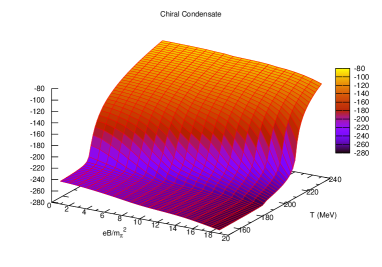
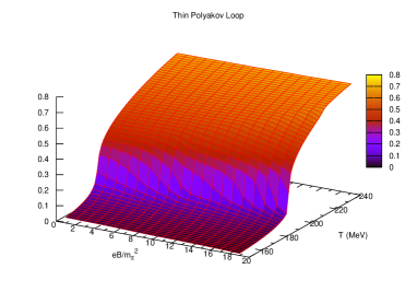
Figure 1: Left panel: Cubic root of the chiral condensate, as a function of temperature and magnetic field. Right panel: Expectation value of the Polyakov loop, $L$, as a function of temperature and magnetic field strength. Results correspond to the P-NJL₈ model.

In this Section, I firstly show the results obtained in [23] within the model with interaction specified in Eq. (2). The numerical values of the parameters can be found in the original reference. The model is named P-NJL₈, following the nomenclature of [17]. Numerical data for the chiral condensate and the Polyakov loop expectation value are shown in Fig. 1. They are obtained from the minimization procedure of the one-loop thermodynamic potential in Eq. (10).

Data on the chiral condensate, left panel of Fig. 1, are in agreement with the magnetic catalysis scenario: both the numerical value of the chiral condensate and the critical temperature, $T_{\chi}$, are increased by the magnetic field. The latter is defined as the value which maximizes $|d\Sigma/dT|$. On the other hand, deconfinement crossover is poorly affected by the magnetic field. The deconfinement temperature, $T_{L}$, is identified with the temperature at which $dL/dT$ is maximum. At $\bm{B}=0$ the two crossovers take place simultaneously at $T=175$ MeV. On the other hand, at $eB=19m_{\pi}^{2}$ the two critical temperatures are split of an amount of $\approx 15\%$. This split is also measured within a different chiral model calculation [27], and persists even in the chiral limit [22].

I briefly compare the results of the P-NJL₈ model, with those obtained within the EPNJL model [17] in which $G_{8}=0$, but an explicit dependence of the NJL coupling on the Polyakov loop is taken into account (I take $L=L^{\dagger}$):

$$G=g\left(1-\alpha_{1}L^{2}-2\alpha_{2}L^{3}\right)~{}.$$ (14)

It has been shown in [39] that this kind of dependence naturally arises in the low energy limit of QCD, see also [40]. The numerical values of $\alpha_{1}$ and $\alpha_{2}$ have been fixed in [17] by a best fit of the available Lattice data at zero and imaginary chemical potential of Ref. [37], $\alpha_{1}=\alpha_{2}\equiv\alpha=0.2\pm 0.05$. The numerical values of the other parameters are standard and can be found in [24].

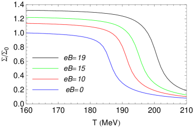
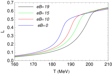
Figure 2: Left panel: Chiral condensate $\Sigma$, measured in units of the chiral condensate at zero temperature and zero field, $\Sigma_{0}$, as a function of temperature, for several values of the magnetic field strength. Right panel: Expectation value of the Polyakov loop, $L$, as a function of temperature, for several values of the magnetic field strength. In the figures, the magnetic fields are measured in units of $m_{\pi}^{2}$. Results correspond to the EPNJL model.

In Fig. 2 I plot data for the chiral condensate $\Sigma$, measured in units of the condensate at vanishing temperature and magnetic field, that is $\Sigma_{0}=2\times(-253~{}\text{MeV})^{3}$, and the expectation value of the Polyakov loop as a function of temperature, computed for several values of the magnetic field strength. The most striking feature of the results is that $T_{L}$ and $T_{\chi}$ are tied together also in a strong magnetic field. At $\bm{B}=0$ the critical temperatures are $T_{P}=T_{\chi}=185.5$ MeV. Besides, at $eB=19m_{\pi}^{2}$, $T_{L}=199$ MeV and $T_{\chi}=201$ MeV. This is due to the fact that the NJL coupling constant in the pseudo-critical region in this model decreases of the amount of the $15\%$ as a consequence of the deconfinement crossover. Therefore, the strength of the interaction responsible for the spontaneous chiral symmetry breaking is strongly affected by the deconfinement, with the obvious consequence that the numerical value of the chiral condensate drops down and the chiral crossover takes place. The picture remains qualitatively and quantitatively unchanged at $eB=30m_{\pi}^{2}$. In this case, $T_{L}=224$ MeV and $T_{\chi}=225$ MeV.

4 The phase diagrams

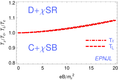
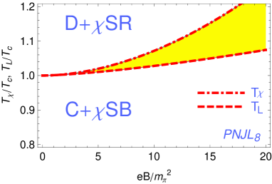
Figure 3: Left panel: Phase diagram in the $eB-T$ plane for the EPNJL model. Temperatures on the vertical axis are measured in units of the pseudo-critical temperature for deconfinement at $eB=0$, namely $T_{c}=185.5$ MeV. Right panel: Phase diagram in the $eB-T$ plane for the PNJL₈ model. Temperatures on the vertical axis are measured in units of the pseudo-critical temperature for deconfinement at $eB=0$, namely $T_{c}=175$ MeV. In both the phase diagrams, $T_{\chi}$, $T_{L}$ correspond to the chiral and deconfinement pseudo-critical temperatures, respectively. The golden region denotes the portion of phase diagram in which hot quark matter is deconfined and chiral symmetry is still broken spontaneously.

Data on deconfinement and chiral symmetry restoration pseudo-critical temperatures are collected in Fig. 3, in the form of a phase diagram in the $eB-T$ plane. The left panel corresponds to the EPNJL model [24]; the right panel corresponds to the results of the P-NJL₈ model [23]. In the figure, the magnetic field is measured in units of $m_{\pi}^{2}$; temperature is measured in units of the deconfinement pseudo-critical temperature at zero magnetic field, namely $T_{B=0}=185.5$ MeV for the EPNJL model, and $T_{B=0}=175$ MeV for the P-NJL₈ model. In the Figure, the golden region corresponds to a phase in which hot quark matter is deconfined, but chiral symmetry is still broken in a non-perturbative way by the chiral condensate.

The most astonishing feature of the phase diagram of the P-NJL₈ model is the entity of the split among the deconfinement and the chiral restoration crossover. The difference with the result of the EPNJL model is that in the former, the entanglement with the Polyakov loop is neglected in the NJL coupling constant. However, the two models share one important feature: both deconfinement and chiral symmetry restoration temperature are increased by a strong magnetic field. They disagree quantitatively, in the sense that the amount of split in the EPNJL model is more modest in comparison with that obtained in the P-NJL₈ model. A similar phase diagram calculation has been performed within the Quark-Meson model in [27], see also the talk by Ana Mizher in this conference. In [27] it is shown that the magnetic field leads to the split of deconfinement and chiral symmetry restoration crossovers, if vacuum fermion fluctuations are properly taken into account; furthermore, both $T_{\chi}$ and $T_{L}$ are enhanced by a magnetic field, in excellent agreement with the behavior of the NJL-like models.

The most recent Lattice data about this kind of study are those of Ref. [25]. In [25], the largest value of magnetic field considered is $eB\approx 0.75$ GeV², which corresponds to $eB/m_{\pi}^{2}\approx 38$. The Lattice data seem to point towards the phase diagram of the EPNJL model, since no split is measured among the two crossovers. On the other hand, the results of [25] might not be definitive: the lattice size might be enlarged, the lattice spacing could be taken smaller (in [25] the lattice spacing is $a=0.3$ fm), and the pion mass could be lowered to its physical value in the vacuum. As a consequence, it will be interesting to compare the model results with more refined data in the future.

5 Conclusions and outlook

In this talk, I have reported on recent results [22, 23, 24] about the phase diagram of hot quark matter in a strong magnetic background. I have considered two models: the P-NJL₈ model and the EPNJL model, following the nomenclature of [17], which differ for the interactions content, but both are tuned to fit Lattice data about QCD thermodynamics at zero and imaginary chemical potential. I have also compared the results with those of [27] in which a Quark-Meson model is used. The most striking similarity among the several models, when the contribution of the fermion determinant is properly kept into account, is that they all support the scenario in which chiral symmetry restoration and deconfinement temperatures are enhanced by a strong magnetic field. The models differ quantitatively for the amount of split measured (very few percent for the EPNJL model, and of the order of $10\%$ for the other models for $eB\approx 20m_{\pi}^{2}$). Furthermore, I have also compared the model results with those obtained on the Lattice [25].

It is fair to admit that the study presented here might have a weak point, namely, it misses a microscopic computation of the dependence of the NJL coupling on the Polyakov loop. Equation (14) is just a particular choice of such a functional dependence. Different functional forms respecting the $C$ and the extended $Z_{3}$ symmetry are certainly possible, and without a rigorous derivation of Eq. (14), it merits to study the topics discussed here using different choices for $G(L)$ in the near future. For these reasons, I prefer to adopt a conservative point of view: it is interesting that the EPNJL model, which is adjusted in order to reproduce Lattice data at zero and imaginary chemical potential, predicts that the two QCD transitions are entangled in a strong magnetic background; however, this conclusion might not be definitive, since there exist other model calculations which share a common basis with EPNJL, and which show a more pronounced split of the QCD transitions in a strong magnetic background. More refined Lattice data will certainly help to discern which of the two scenarios is the most favorable.

The results collected here suggest several continuation lines. Firstly, it is worth to compute the magnetic susceptibility of the chiral condensate [41] within chiral models, which allow to treat self-consistently the spontaneous chiral symmetry breaking in a magnetic field. Besides, the technical machinery used here can be easily applied to a microscopic study of the spectral properties of mesons in strong magnetic field, in particular of $\rho$ mesons following [29]. Furthermore, it would be interesting to make a complete analytical study of the chiral limit, to estimate the effect of the magnetic field on the universality class of two-flavor QCD. Finally, the phase diagram with chiral chemical potential deserves further study, following [22, 43].

- [1] P. de Forcrand and O. Philipsen, JHEP 0701, 077 (2007); JHEP 0811, 012 (2008); PoS LATTICE2008, 208 (2008).
- [2] Y. Aoki et al., Nature 443, 675 (2006); Y. Aoki, S. Borsanyi, S. Durr, Z. Fodor, S. D. Katz, S. Krieg and K. K. Szabo, JHEP 0906, 088 (2009); S. Borsanyi et al., S. Borsanyi et al., JHEP 1009 (2010) 073;
- [3] A. Bazavov et al., Phys. Rev. D 80, 014504 (2009).
- [4] M. Cheng et al., Phys. Rev. D 81, 054510 (2010).
- [5] F. Karsch, E. Laermann and A. Peikert, Nucl. Phys. B 605, 579 (2001); F. Karsch, Lect. Notes Phys. 583, 209 (2002); O. Kaczmarek and F. Zantow, Phys. Rev. D 71, 114510 (2005).
- [6] C. S. Fischer, Phys. Rev. Lett. 103, 052003 (2009); C. S. Fischer and J. A. Mueller, Phys. Rev. D 80, 074029 (2009); C. S. Fischer, A. Maas and J. A. Muller; Eur. Phys. J. C 68, 165 (2010). A. C. Aguilar and J. Papavassiliou, arXiv:1010.5815 [hep-ph]; C. Feuchter and H. Reinhardt, Phys. Rev. D 70, 105021 (2004); Phys. Rev. D 71, 105002 (2005). M. Leder, J. M. Pawlowski, H. Reinhardt and A. Weber, arXiv:1006.5710 [hep-th]; J. Braun, Eur. Phys. J. C 64, 459 (2009) [arXiv:0810.1727 [hep-ph]]; J. Braun, L. M. Haas, F. Marhauser and J. M. Pawlowski, arXiv:0908.0008 [hep-ph]; M. Frasca, Phys. Lett. B 670, 73 (2008); Mod. Phys. Lett. A 24 (2009) 2425; arXiv:1007.4479 [hep-ph].
- [7] Y. Nambu and G. Jona-Lasinio, Phys. Rev. 122, 345 (1961); Y. Nambu and G. Jona-Lasinio, Phys. Rev. 124, 246 (1961).
- [8] U. Vogl and W. Weise, Prog. Part. Nucl. Phys. 27, 195 (1991); S. P. Klevansky, Rev. Mod. Phys. 64, 649 (1992); T. Hatsuda and T. Kunihiro, Phys. Rept. 247, 221 (1994); M. Buballa, Phys. Rept. 407, 205 (2005).
- [9] P. N. Meisinger and M. C. Ogilvie, Phys. Lett. B 379, 163 (1996).
- [10] K. Fukushima, Phys. Lett. B 591, 277 (2004).
- [11] A. M. Polyakov, Phys. Lett. B 72, 477 (1978); L. Susskind, Phys. Rev. D 20, 2610 (1979); B. Svetitsky and L. G. Yaffe, Nucl. Phys. B 210, 423 (1982); B. Svetitsky, Phys. Rept. 132, 1 (1986).
- [12] C. Ratti, M. A. Thaler and W. Weise, Phys. Rev. D 73, 014019 (2006).
- [13] S. Roessner, C. Ratti and W. Weise, Phys. Rev. D 75, 034007 (2007).
- [14] H. Abuki, R. Anglani, R. Gatto, G. Nardulli and M. Ruggieri, Phys. Rev. D 78, 034034 (2008).
- [15] Y. Sakai, K. Kashiwa, H. Kouno and M. Yahiro, Phys. Rev. D 77, 051901 (2008); Phys. Rev. D 78, 036001 (2008); Y. Sakai, K. Kashiwa, H. Kouno, M. Matsuzaki and M. Yahiro, arXiv:0902.0487 [hep-ph]; K. Kashiwa, H. Kouno, M. Matsuzaki and M. Yahiro, Phys. Lett. B 662, 26 (2008).
- [16] H. Abuki, M. Ciminale, R. Gatto, N. D. Ippolito, G. Nardulli and M. Ruggieri, Phys. Rev. D 78, 014002 (2008).
- [17] Y. Sakai, T. Sasaki, H. Kouno and M. Yahiro, Phys. Rev. D 82, 076003 (2010).
- [18] T. Hell, S. Roessner, M. Cristoforetti and W. Weise, Phys. Rev. D 79, 014022 (2009).
- [19] T. K. Herbst, J. M. Pawlowski and B. J. Schaefer, arXiv:1008.0081 [hep-ph].
- [20] V. Skokov, B. Friman and K. Redlich, arXiv:1008.4570 [hep-ph].
- [21] T. Kahara and K. Tuominen, Phys. Rev. D 78, 034015 (2008); T. Kahara and K. Tuominen, Phys. Rev. D 80, 114022 (2009); T. Kahara and K. Tuominen, arXiv:1006.3931 [hep-ph].
- [22] K. Fukushima, M. Ruggieri and R. Gatto, Phys. Rev. D 81, 114031 (2010).
- [23] R. Gatto and M. Ruggieri, Phys. Rev. D 82, 054027 (2010).
- [24] R. Gatto and M. Ruggieri, arXiv:1012.1291 [hep-ph].
- [25] M. D’Elia, S. Mukherjee and F. Sanfilippo, Phys. Rev. D 82, 051501 (2010).
- [26] P. V. Buividovich, M. N. Chernodub, E. V. Luschevskaya and M. I. Polikarpov, Phys. Rev. D 81, 036007 (2010); Phys. Lett. B 682, 484 (2010); Nucl. Phys. B 826, 313 (2010).
- [27] A. J. Mizher, M. N. Chernodub and E. S. Fraga, Phys. Rev. D 82, 105016 (2010).
- [28] S. P. Klevansky and R. H. Lemmer, Phys. Rev. D 39, 3478 (1989); H. Suganuma and T. Tatsumi, Annals Phys. 208, 470 (1991); I. A. Shushpanov and A. V. Smilga, Phys. Lett. B 402, 351 (1997); D. N. Kabat, K. M. Lee and E. J. Weinberg, Phys. Rev. D 66, 014004 (2002); T. D. Cohen, D. A. McGady and E. S. Werbos, Phys. Rev. C 76, 055201 (2007); V. P. Gusynin, V. A. Miransky and I. A. Shovkovy, Nucl. Phys. B 462, 249 (1996); V. A. Miransky and I. A. Shovkovy, Phys. Rev. D 66, 045006 (2002); K. G. Klimenko, Theor. Math. Phys. 89, 1161 (1992) [Teor. Mat. Fiz. 89, 211 (1991)]; K. G. Klimenko, Z. Phys. C 54, 323 (1992); K. G. Klimenko, Theor. Math. Phys. 90, 1 (1992) [Teor. Mat. Fiz. 90, 3 (1992)]; B. Hiller, A. A. Osipov, A. H. Blin and J. da Providencia, SIGMA 4, 024 (2008); N. O. Agasian and S. M. Fedorov, Phys. Lett. B 663, 445 (2008); E. S. Fraga and A. J. Mizher, Phys. Rev. D 78, 025016 (2008).
- [29] M. N. Chernodub, Phys. Rev. D 82, 085011 (2010); arXiv:1101.0117 [hep-ph].
- [30] I. E. Frolov, V. C. Zhukovsky and K. G. Klimenko, Phys. Rev. D 82, 076002 (2010).
- [31] D. E. Kharzeev, L. D. McLerran and H. J. Warringa, Nucl. Phys. A 803, 227 (2008).
- [32] V. Skokov, A. Y. Illarionov and V. Toneev, Int. J. Mod. Phys. A 24, 5925 (2009).
- [33] P. V. Buividovich, M. N. Chernodub, E. V. Luschevskaya and M. I. Polikarpov, Phys. Rev. D 80, 054503 (2009); M. Abramczyk, T. Blum, G. Petropoulos and R. Zhou, PoS LAT2009, 181 (2009).
- [34] K. Fukushima, D. E. Kharzeev and H. J. Warringa, Phys. Rev. D 78, 074033 (2008).
- [35] K. I. Kondo, Phys. Rev. D 82, 065024 (2010).
- [36] M. Frasca, arXiv:0803.0319 [hep-th]; arXiv:1002.4600 [hep-ph].
- [37] M. D’Elia and F. Sanfilippo, Phys. Rev. D 80, 111501 (2009). C. Bonati, G. Cossu, M. D’Elia and F. Sanfilippo, arXiv:1011.4515 [hep-lat].
- [38] V. I. Ritus, Annals Phys. 69, 555 (1972); C. N. Leung and S. Y. Wang, Nucl. Phys. B 747, 266 (2006).
- [39] K. I. Kondo, Phys. Rev. D 82, 065024 (2010).
- [40] M. Frasca, arXiv:0803.0319 [hep-th]; arXiv:1002.4600 [hep-ph].
- [41] B. L. Ioffe and A. V. Smilga, Nucl. Phys. B 232, 109 (1984).
- [42] A. A. Osipov, B. Hiller and J. da Providencia, Phys. Lett. B 634, 48 (2006).
- [43] M. N. Chernodub and A. S. Nedelin, arXiv:1102.0188 [hep-ph].