Variational study of the quantum phase transition in bilayer Heisenberg model with Bosonic RVB wave function

Abstract

We study the ground state phase diagram of the bilayer Heisenberg model on square lattice with a Bosonic RVB wave function. The wave function has the form of a Gutzwiller projected Schwinger Boson mean field ground state and involves two variational parameters. We find the wave function provides an accurate description of the system on both sides of the quantum phase transition. Especially, through the analysis of the spin structure factor, ground state fidelity susceptibility and the Binder moment ratio $Q_{2}$, a continuous transition from the antiferromagnetic ordered state to the quantum disordered state is found at the critical coupling of $\alpha_{c}=J_{\perp}/J_{\parallel}\approx 2.62$, in good agreement with the result of quantum Monte Carlo simulation. The critical exponent estimated from the finite size scaling analysis($1/\nu\approx 1.4$) is consistent with that of the classical 3D Heisenberg universality class.

I I. Introduction

The study of quantum phase transition is a central issue in modern condensed matter physics. It is widely believed that the Ginzburg-Landau-Wilson theory for classical phase transition may fail to describe the quantum phase transition as a result of the quantum interference effect between classical paths(the Berry phase effect). Recently, the concepts of quantum order and de-confined quantum criticality are put forward theoretically. On the experimental side, the study of quantum phase transition plays an important role in areas ranging from high-Tc cuprates, heavy Fermion systems, to the cold atom systemsSachdev1 .

The bilayer Heisenberg model(BHM) on square lattice is a standard model for the study of quantum phase transition. With the increase of the interlayer coupling($J_{\perp}$) over the intralayer coupling($J_{\parallel}$), the ground state of the system evolves from a state with antiferromagnetic long rang order to a quantum disordered state through a continuous phase transition. Much theoretical and numerical efforts have been devoted to the study of this quantum phase transition.

On theoretical side, perturbative calculations starting from both the ordered side(spin wave expansion)spinwave and the disordered side(the bond operator expansion)bond have been applied to the system. However, due to the biased nature of pertubative methods, none of them can give an accurate description of the system in the near vicinity of the quantum phase transition. The problem is also treated with the Schwinger Boson mean field theoryschwinger ; Millis . Although the theory does predict a phase transition between the antiferromagnetic ordered state and the quantum disordered state, the nature of the transition is incorrect. The mean field theory predicts a discontinues dimerization transition around $J_{\perp}/J_{\parallel}=4.62$ into a state composed of independent interlayer dimers, while in the real system, the intralayer correlation is nonzero for any finite $J_{\perp}/J_{\parallel}$.

On numerical side, the model is thoroughly studied by a variety of methods including the high temperature series expansionseries and the quantum Monte Carlo simulation(Stochastic series expansion)qmc ; Wang . These numerical works confirm the existence of the quantum critical point around $\alpha=J_{\perp}/J\approx 2.52$. The critical exponents is found to be consistent with that of the classical 3D Heisenberg universality class, indicating the irrelevance of the Berry phase effect in this phase transition.

As the quantum phase transition occurs at zero temperature, it is natural to find a description of it in terms of an explicit ground state wave function. The variational approach to quantum phase transition has the virtue that it focus directly on the zero temperature behavior of the system and provides much more detailed information on the quantum critical behavior. In this regard, a RVB-type variational wave functionRVB ; loop had been applied to the study of the quantum phase transition in the BHM. The wave function is derived from Gutzwiller projection of Schwinger Boson mean field ground state. It is well known that such a RVB wave function can describe both the magnetic ordered and the quantum disordered state. Thus, it has the potential to provide an unbiased description of the quantum phase transition in BHM. The same type of variational wave function has been successfully applied to the study of the single layer two-dimensional Heisenberg modelRVB ; schwinger1 . However, for the BHM, the variational calculation in Yoshioka using such a wave function predicts a critical coupling $\alpha_{c}=3.51$, which is a very bad estimate as compared to the result of numerical simulation. A central issue to be addressed in this paper is to understand why the Bosonic RVB state, which works so well on square lattice, fails for the BHM and how to improve it.

In this paper, we propose a RVB-type variational wave function with two variational parameters for the BHM. Similar to Yoshioka , our wave function is derived from Gutzwiller projected Schwinger Boson mean field state. However, in our theory the intralayer RVB pairing and interlayer RVB pairing are treated as two independent variational parameters, rather than been determined by mean field self-consistent equations. We find our variational wave function provides an accurate description of the quantum phase transition of the BHM. We find the the transition is continuous. By analyzing the spin structure factor, ground state fidelity susceptibility and Binder moment ratio $Q_{2}$, the critical coupling strength is estimated to be $\alpha_{c}\approx 2.62$, in good agreement with those determined from the numerical simulation. The critical exponent estimated from the scaling analysis of the $Q_{2}$ data is also consistent wit that of the classical 3D Heisenberg universality class. Our result indicates that the Bosonic RVB wave function derived from Gutzwiller projection of the Schwinger Boson mean field state can provides accurate description of the quantum phase transition in quantum antiferromagnets. We also find that the failure of the Schwinger Boson mean field theory originates from the overestimation of the tendency to form interlayer dimers, which is again caused by the relaxation of the no double occupancy constraint.

The paper is organized as follows. In section II, we introduce the BHM and the Bosonic RVB wave function. In section III, we present the numerical method to do calculation on such wave functions. In section IV, we present the numerical results and determine the critical point of the phase transition by analyzing the results of fidelity susceptibility and Binder moment ratio. In section V, we present a discussion on related issues and conclude this paper.

II II. The bilayer Heisenberg model and the RVB-type variational wave function

The model(BHM) we study in this paper is given by

$$\mathrm{H}=J_{\parallel}\sum_{<i,j>,\mu}\vec{\mathrm{S}}_{i}^{\mu}\cdot\vec{\mathrm{S}}_{j}^{\mu}+J_{\perp}\sum_{i}\vec{\mathrm{S}}_{i}^{1}\cdot\vec{\mathrm{S}}_{i}^{2},$$ (1)

where $\vec{\mathrm{S}}_{i}^{\mu}$ denotes the spin operator at site $i$ of layer $\mu(=1,2)$. $\sum_{<i,j>}$ means the summation over nearest-neighboring sites on the square lattice of each layer. $\alpha=J_{\perp}/J_{\parallel}$ is the only dimensionless parameter of the model. When $\alpha=0$, the model describes two decoupled two-dimensional Heisenberg model, each of which are antiferromagnetic ordered at zero temperature. When $\alpha\rightarrow\infty$, the system reduces to N decoupled interlayer dimers and the system is in a trivial quantum disordered state. A continuous quantum phase transition connects these two limits. Earlier numerical simulation shows that the phase transition occurs around $\alpha_{c}=2.52$qmc ; Wang .

The Bosonic RVB wave function we will adopt in this study is made of coherent superposition of spin singlet configurations on the lattice and can be written as

$$|\mathrm{RVB}\rangle=\sum_{\{i_{k},j_{k}\}}A(\{i_{k},j_{k}\})\prod_{k=1}^{N/2}S(i_{k},j_{k}),$$ (2)

in which $S(i_{k},j_{k})=\frac{1}{\sqrt{2}}(\uparrow_{i_{k}}\downarrow_{j_{k}}-\downarrow_{i_{k}}\uparrow_{j_{k}})$ denotes the spin singlet pair between site $i_{k}$ and $j_{k}$. $A(\{i_{k},j_{k}\})$ are the coefficients of the coherent superposition. In our case, $A(\{i_{k},j_{k}\})$ can be written in a factorizeable form $A(\{i_{k},j_{k}\})=\prod_{k=1}^{N/2}a_{i_{k},j_{k}}$

The wave function Eq.(2) can be used directly as variational state for quantum antiferromagnet. A more efficient and intuitively more attractive way to generate the RVB wave function is by Gutzwiller projection of Schwinger Boson mean field state. This approach is used to study two-dimensional Heisenberg model and is proved to be very successful. However, direct application of the approach to the BHM results in unsatisfactory results.

Here, we will adopt the form of the Gutzwiller projected Schwinger Boson mean field state, but regard the mean field order parameters(intralayer and interlayer RVB pairing amplitudes) as free variational parameters, rather than been determined from the mean field self-consistent equations. The reason for such a choice is as follows. In the mean field treatment, the no double occupancy constraint is relaxed. As a result, the quantitative prediction of the mean field theory is not reliable. For example, the mean field equation predicts an un-physical dimerization transition for BHM at $\alpha\approx 4.62$, whose origin can be traced back to the overestimation the tendency to form interlayer dimers, which is again related to the relaxation of the local constraint.

In the Schwinger Boson representationschwinger , the spin operator is written as

$$\vec{\mathrm{S}}=\frac{1}{2}\sum_{\alpha,\beta=1,2}b^{\dagger}_{\alpha}\vec{\sigma}_{\alpha,\beta}b_{\beta},$$ (3)

in which $b_{\alpha}$ is a Boson operator, $\vec{\sigma}$ is the Pauli matrix. Eq.(3) is a faithful representation of the spin algebra provided that the Bosonic particle satisfy the no double occupancy constraint

$$\sum_{\alpha}b^{\dagger}_{\alpha}b_{\alpha}=1.$$ (4)

The BHM written in terms of the Schwinger Boson operators reads

$$\mathrm{H}= - J_{\parallel}\sum_{<i,j>,\mu}\hat{\Delta}_{i,j}^{\mu\dagger}\hat{\Delta}_{i,j}^{\mu}-J_{\perp}\sum_{i}\hat{\Delta}_{i}^{\dagger}\hat{\Delta}_{i}$$ (5)

$$- \sum_{i,\mu}\lambda_{i,\mu}(n_{i,\mu}-1)$$

in which

$$\hat{\Delta}_{i,j}^{\mu} = \frac{1}{\sqrt{2}}(b_{i,\mu,\uparrow}b_{j,\mu,\downarrow}-b_{i,\mu,\downarrow}b_{j,\mu,\uparrow})$$

$$\hat{\Delta}_{i} = \frac{1}{\sqrt{2}}(b_{i,1,\uparrow}b_{i,2,\downarrow}-b_{i,1,\downarrow}b_{i,2,\uparrow})$$ (6)

denote the intralayer and interlayer RVB pairing operator, $n_{i,\mu}=\sum_{\alpha=\uparrow,\downarrow}b_{i,\mu,\alpha}^{\dagger}b_{i,\mu,\alpha}$. The Largrange multiplier $\lambda_{i,\mu}$ is introduced to keep track of the local constraint.

In the mean field theory, we treat $\lambda_{i,\mu}=\lambda$ as a constant and decouple the interaction term using the following mean field order parameters $\Delta_{\parallel}=\langle\hat{\Delta}_{i,j}^{1}\rangle=\langle\hat{\Delta}_{i,j}^{2}\rangle$ and $\Delta_{\perp}=\langle\hat{\Delta}_{i}\rangle$. The mean field Hamiltonian reads(up to a constant)

$$\mathrm{H}_{\mathrm{MF}} = -J_{\parallel}\Delta_{\parallel}\sum_{<i,j>,\mu}(\hat{\Delta}_{i,j}^{\mu\dagger}+\hat{\Delta}_{i,j}^{\mu})$$ (7)

$$-J_{\perp}\Delta_{\perp}\sum_{i}(\hat{\Delta}_{i}^{\dagger}+\hat{\Delta}_{i})-\lambda\sum_{i,\mu}n_{i,\mu}.$$

The mean field ground state of Eq.(7) reads

$$|G\rangle=\exp\Bigl{[}\sum_{i,j;\mu,\nu} a_{i\mu,j\nu} (b_{i\mu,\uparrow}^{\dagger}b_{j\nu,\downarrow}^{\dagger}-b_{i\mu,\downarrow}^{\dagger}b_{j\nu,\uparrow}^{\dagger})\Bigr{]}\Bigl{|}0\Bigr{\rangle},$$ (8)

in which $|0\rangle$ denotes the vacuum of the Schwinger Boson. $a_{i\mu,j\nu}$ represents the RVB amplitude between site $i$ in $\mu$ layer and site $j$ in $\nu$ layer. As a result of the bipartite nature of the system, the RVB amplitude is nonzero only for sites belonging to different sublattices. Thus for $\mu=\nu$, $a_{i\mu,j\nu}$ is nonzero only when $i,j$ have different parity, while for $\mu\neq\nu$ the reverse is true. The intralayer and interlayer RVB amplitudes are given by($a_{i1,j1}=a_{i2,j2},a_{i1,j2}=a_{i2,j1}$ by symmetry)

$$a_{i1,j1}=\frac{1}{N}\sum_{\vec{k}}[\xi(k)+\eta(k)]\exp(i\vec{k}\cdot\vec{r}_{i,j})$$

$$a_{i1,j2}=\frac{1}{N}\sum_{\vec{k}}[\xi(k)-\eta(k)]\exp(i\vec{k}\cdot\vec{r}_{i,j}),$$ (9)

in which

$$\xi(k)=\frac{c_{1}\gamma(k)+c_{2}}{1+\sqrt{1-(c_{1}\gamma(k)+c_{2})^{2}}}$$

$$\eta(k)=\frac{c_{1}\gamma(k)-c_{2}}{1+\sqrt{1-(c_{1}\gamma(k)-c_{2})^{2}}},$$

here $c_{1}=4J_{\parallel}\Delta_{\parallel}/\sqrt{2}\lambda$, $c_{2}=J_{\perp}\Delta_{\perp}/\sqrt{2}\lambda$, $\gamma(k)=(\cos(k_{x})+\cos(k_{y}))/2$.

The Bosonic RVB wave function adopted in this study is given by Gutzwiller projection of the mean field ground state into the physical subspace satisfying the local constraint,

$$|G\rangle=P_{G}\Bigl{[}\sum_{i,j;\mu,\nu} a_{i\mu,j\nu} (b_{i\mu,\uparrow}^{\dagger}b_{j\nu,\downarrow}^{\dagger}-b_{i\mu,\downarrow}^{\dagger}b_{j\nu,\uparrow}^{\dagger})\Bigr{]}^{N/2}\Bigl{|}0\Bigr{\rangle}$$

. (10)

Here $P_{G}$ denotes the Gutzwiller projection and $N$ is the number of lattice sites. The mean field ground state contains two dimensionless parameters, namely $c_{1}$ and $c_{2}$. In the mean field theory, both of them are determined by the mean field self-consistent equations. Here we regard them as two independent variational parameters. This is the key difference between our theory and that of Yoshioka .

The proposed wave function Eq.(10) can describe both the magnetic ordered and the quantum disordered state. As can be seen from Eq.(9), as $c_{1}+c_{2}\rightarrow 1$, both $a_{i1,j1}$ and $a_{i1,j2}$ becomes long ranged and the wave function describes a state with antiferromagnetic long range order. On the other hand, when $c_{1}+c_{2}$ deviates from 1, the RVB amplitudes $a_{i1,j1}$ and $a_{i1,j2}$ become short ranged and the corresponding wave function describes a quantum disordered state. In fact, $c_{1}+c_{2}=1$ is nothing but the Bose condensation condition in the mean field theory.

On general grounds, we expect the interlayer pairing $c_{2}$ to increase with $\alpha$ and the intralayer pairing $c_{1}$ to decrease with $\alpha$. The transition between the antiferromagnetic ordered state and the quantum disordered state is signaled by the deviation of $c_{1}+c_{2}$ from 1. These expectations are confirmed in the numerical calculation.

III III. The numerical techniques

The Bosonic RVB wave function Eq.(10) can be studied by the standard loop gas Monte Carlo algorithmloop . In this algorithm, the calculation of expectation value of a physical quantity $\hat{A}$(for example the energy) is done as follows

$$\frac{\langle G|\hat{A}|G\rangle}{\langle G|G\rangle}=\frac{\sum_{\gamma,\gamma^{\prime}}\psi^{*}_{\gamma}\psi_{\gamma^{\prime}}\langle\gamma|\gamma^{\prime}\rangle\frac{\langle\gamma|\hat{A}|\gamma^{\prime}\rangle}{\langle\gamma|\gamma^{\prime}\rangle}}{\sum_{\gamma,\gamma^{\prime}}\psi^{*}_{\gamma}\psi_{\gamma^{\prime}}\langle\gamma|\gamma^{\prime}\rangle}.$$ (11)

Here $|\gamma\rangle$ denotes the valence bond basis vector and is given by $|\gamma\rangle=\prod_{(i,j)\in\gamma}S(i,j)$. $\psi_{\gamma}$ is the corresponding amplitude and is given by $\psi_{\gamma}=\prod_{(i,j)\in\gamma}a_{i,j}$. The overlap between two valence bond basis vectors $|\gamma\rangle$ and $|\gamma^{\prime}\rangle$ can be graphically interpreted as a loop gas on the lattice by fusing the valence bonds in the two basis vectors. It is easy to show that $\langle\gamma|\gamma^{\prime}\rangle=2^{N_{L}}$, where $N_{L}$ is the number of loops in the transition graph between $|\gamma\rangle$ and $|\gamma^{\prime}\rangle$.

As the system is bipartite, the RVB amplitude $a_{i1,j1}$ and $a_{i1,j2}$ are in fact positive definite and the wave function Eq.(10) satisfy the Marshall sign ruleloop . For this reason, we can interpret $W(\gamma,\gamma^{\prime})=\frac{\psi^{*}_{\gamma}\psi_{\gamma^{\prime}}\langle\gamma|\gamma^{\prime}\rangle}{\sum_{\gamma,\gamma^{\prime}}\psi^{*}_{\gamma}\psi_{\gamma^{\prime}}\langle\gamma|\gamma^{\prime}\rangle}$ as a normalized probability in the space of loop gas and can draw samples on it with the standard Monte Carlo method. The calculation of $\frac{\langle\gamma|\hat{A}|\gamma^{\prime}\rangle}{\langle\gamma|\gamma^{\prime}\rangle}$ is easy for $\hat{A}=\vec{\mathrm{S}}_{i}\cdot\vec{\mathrm{S}}_{j}$ and the result reads

$$\langle\vec{\mathrm{S}}_{i}\cdot\vec{\mathrm{S}}_{j}\rangle=\left\{\begin{array}[]{ll}-\frac{3}{4},&\hbox{$i,j\in$ same loop, different sublattices;}\\ \frac{3}{4},&\hbox{$i,j\in$ same loop, same sublattice;}\\ 0,&\hbox{otherwise.}\end{array}\right.$$ (15)

Thus both the energy and spin structure factor can be easily calculated with the standard Monte Carlo procedure in the loop gas space.

To determine the optimal value of the variational parameter $c_{1}$ and $c_{2}$, we calculate the expectation value of the energy and of its gradients in the parameter space $(c_{1},c_{2})$ on a finite lattice. It is useful to note that the gradients of energy can be directly simulated by the loop gas Monte Carlo method also. Its expression is given by

$$\frac{\partial E(c_{1},c_{2})}{\partial c_{1,2}} = \left\langle\Bigl{(}\sum_{(i,j)\in\gamma,\gamma^{\prime}}\frac{\partial\ln a_{i,j}}{\partial c_{1,2}}\Bigr{)}\frac{\langle\gamma|\hat{H}|\gamma^{\prime}\rangle}{\langle\gamma|\gamma^{\prime}\rangle}\right\rangle_{L}$$ (16)

$$- E(c_{1},c_{2})\left\langle\sum_{(i,j)\in\gamma,\gamma^{\prime}}\frac{\partial\ln a_{i,j}}{\partial c_{1,2}}\right\rangle_{L},$$

where $\langle\rangle_{L}$ denotes average over the loop gas configurations with the weight $W(\gamma,\gamma^{\prime})$.

We have used $10^{8}$ samples to calculate the energy and its gradients to determine the optimized values for $c_{1}$ and $c_{2}$. The boundary condition of the finite lattice is set to be periodic in both directions. The calculation is done on a lattice with size up to $20\times 20\times 2$, at which we find the critical coupling converges to $\alpha_{c}\approx 2.62$.

IV IV. The numerical results

The optimized value for the parameter $c_{1}$ and $c_{2}$ as functions of the coupling constant $\alpha$ are shown in Fig.1. As $\alpha$ increases, the interlayer RVB pairing strength $c_{2}$ increases at the expense of the intralayer RVB pairing strength $c_{1}$. The result is obtained on a $20\times 20\times 2$ lattice. It is found that the optimized values deviate significantly from the mean field predictions, especially for large value of $\alpha$. For example, the mean field theory predicts that $\Delta_{\perp}$ would reach twice the value of $\Delta_{\parallel}$ around $\alpha=4$. However, the variational theory predicts that $\Delta_{\perp}$ is slightly smaller than $\Delta_{\parallel}$ around $\alpha=4$. Thus, the mean field theory overestimates greatly the tendency to form interlayer dimer at large $\alpha$.

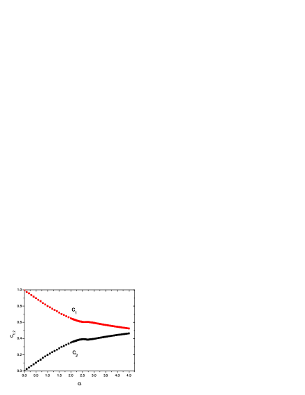
Figure 1: The optimized value for the intralayer and interlayer RVB pairing strength $c_{1}$ and $c_{2}$ as functions of the coupling constant $\alpha$.

To better understand the evolution of the variational parameters as functions of $\alpha$, we plot the value of the $a=c_{1}+c_{2}$ as a function of $\alpha$ in Fig.2. As we have shown above, the quantum phase transition between the magnetic ordered state and the quantum disordered state in our variational theory is solely controlled by the value of $a$. The value of $a$ is seen to deviate from unity around $2.6$, at which the Bose condensate of the spinon is gone.

Figure 2: The optimized value for the variational parameter $a=c_{1}+c_{2}$, which controls the order-disorder transition of BHM.

To further characterize the quantum phase transition and determine the value of the critical coupling $\alpha_{c}$, we study the following three kinds of quantities: the spin structure factor at the ordering wave vector, the fidelity susceptibility of the ground state and the Binder moment ratio $Q_{2}$.

IV.1 A. Spin Structure Factor

For a finite system, the spontaneous magnetization can be defined in a spin rotational invariant way as the square root of the spin structure factor at the magnetic Bragg vector. For BHM, the Bragg vector is $\vec{Q}=(\pi,\pi,\pi)$. The spin structure factor is defined as

$$S(\vec{q})=\frac{1}{N}\sum_{i,j}\langle\vec{\mathrm{S}}_{i}\cdot\vec{\mathrm{S}}_{j}\rangle\exp(i\vec{q}\cdot\vec{r}_{i,j})$$ (17)

For $q=Q$, we have

$$M^{2}=NS(\vec{Q})=\sum_{i,j}(-1)^{i-j}\langle\vec{\mathrm{S}}_{i}\cdot\vec{\mathrm{S}}_{j}\rangle$$ (18)

In the quantum disordered state, as the spin correlation length is finite, $S(\vec{Q})$ is of order one. However, in the magnetic ordered state, $S(\vec{Q})$ should scale like $N$ and thus $M$ is an extensive quantity.

The result of the spin structure factor for a $20\times 20\times 2$ system is shown in Fig.3. An order-disorder transition can be seen around $2.5$. However, the signature of phase transition in the spin structure factor is not sharp enough for an accurate determination of the critical coupling strength. The transition is rounded into a crossover as a result of the finite size effect. For this reason, we need some other quantities that are more sensitive to the transition to determine the critical coupling.

Figure 3: The spin structure factor at the antiferromagnetic ordering wave vector as a function of $\alpha$ for a system with $L=20$.

IV.2 B. Fidelity Susceptibility

The concept of fidelity susceptibility is introduced to describe the sensitivity of the ground state to the variation of the parameters in Hamiltonianfidelity and is expected to reach its maximum at the critical coupling of a quantum phase transition, where the ground state is the most susceptible to the variation of the controlling parameters of the phase transition. The fidelity susceptibility is defined in the following manner for a system with only one parameter $\alpha$,

$$\chi_{f}=-2\lim_{\delta\alpha\rightarrow 0}\frac{\ln|O(\alpha,\delta\alpha)|}{(\delta\alpha)^{2}},$$ (19)

in which $O(\alpha,\delta\alpha)=\langle\Psi_{\alpha}|\Psi_{\alpha+\delta\alpha}\rangle$ denotes the overlap between the normalized ground state vector for parameter value $\alpha$ and $\alpha+\delta\alpha$.

In our variational theory, the fidelity susceptibility can be calculated directly. We first fit the optimized variational parameters as functions of $\alpha$ and then calculate the overlap between variational ground states for nearby values of $\alpha$. The overlap between the Bosonic RVB states is calculated in the following way.

$$\frac{\langle\Psi|\Psi^{\prime}\rangle}{\langle\Psi|\Psi\rangle}=\frac{\sum_{\gamma,\gamma^{\prime}}\psi^{*}_{\gamma}\psi_{\gamma^{\prime}}\langle\gamma|\gamma^{\prime}\rangle\frac{\psi^{\prime}_{\gamma^{\prime}}}{\psi_{\gamma^{\prime}}}}{\sum_{\gamma,\gamma^{\prime}}\psi^{*}_{\gamma}\psi_{\gamma^{\prime}}\langle\gamma|\gamma^{\prime}\rangle}.$$ (20)

In our calculation, we have set $\delta\alpha=0.01$. The result for the fidelity susceptibility for systems of several sizes are shown in Fig.4. A pronounced peak appears around $\alpha=2.6$. Fig.5 shows the peak position extracted from Fig.4 as a function of the system size $L$. It is found that the peak position converges rapidly to its thermodynamic limit value $\alpha_{c}\approx 2.62$ when $L>10$.

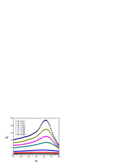
Figure 4: The fidelity susceptibility for system of size $L=6,8,10,14,16,18$ and $20$ as functions of $\alpha$. The finite difference used to calculate the fidelity susceptibility is $\delta\alpha=0.01$.

Figure 5: The critical coupling strength $\alpha_{c}$ determined from the peak position of the fidelity susceptibility. The peak position is seen to converge rapidly to its thermodynamic limit when $L>10$. The error bars are smaller than the size of the symbols.

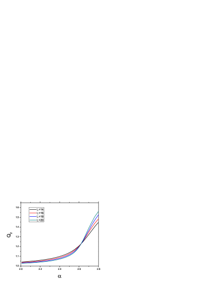
Figure 6: The Binder moment ratio $Q_{2}$ for $L=14,16,18$ and $20$ as functions of $\alpha$.

IV.3 C. Binder Moment Ratio $Q_{2}$

To confirm the result derived from the fidelity susceptibility, we calculate the Binder moment ratio $Q_{2}$Wang ; Binder . The Binder moment ratio $Q_{2}$ is a dimensionless quantity defined in the following manner,

$$Q_{2}=\frac{\langle\hat{S}_{Q}^{2}\rangle}{\langle\hat{S}_{Q}\rangle^{2}},$$ (21)

in which $\hat{S}_{Q}=\sum_{i,j}(-1)^{i-j}\vec{S}_{i}\cdot\vec{S}_{j}$. Note our definition of $Q_{2}$ is slightly different from the standard one in that it is defined in a spin rotational invariant way, while in the standard definition only the $z$-component of the moment is used. The Binder moment ratio is very useful in the analysis of the critical properties as it is universal near the critical point. More specifically, it can be expressed as a universal scaling function of $tL^{1/\nu}$, where $t=(\alpha-\alpha_{c})$ and $\nu$ is the critical exponent for correlation length.

The results of $Q_{2}$ for system with $L=14,16,18$ and $20$ are shown in Fig.6. It is found that all curves cross with each other at approximately the same value of $\alpha$, in accordance with the scaling hypothesis. The estimated value of the critical coupling strength is $2.62$, in good agrement with that estimated from the fidelity susceptibility data. The $Q_{2}$ value at the crossing point is found to be approximately $1.23$, close but smaller than the value(1.29) estimated from the quantum Monte Carlo simulation with the standard definition of $Q_{2}$. Such a difference may be caused by the difference in the definitions of $Q_{2}$.

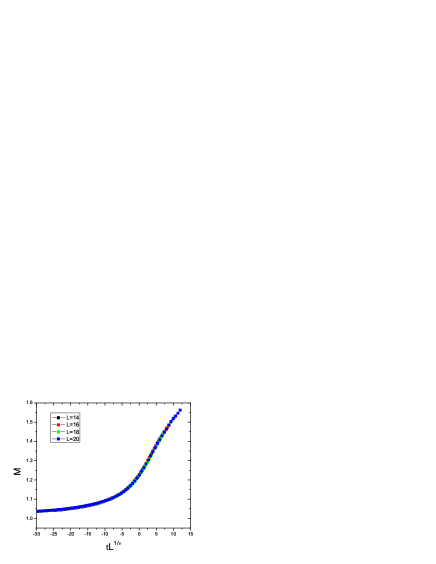
Figure 7: Scaling of the Binder moment ratio $Q_{2}$ data for $L=14,16,18$ and $20$. Here $t=\alpha-\alpha_{c}$

Fig.7 shows the scaling of the $Q_{2}$ data with the scaling form $Q_{2}=M(tL^{1/\nu})$, where $t=\alpha-\alpha_{c}$ and $\nu$ is the exponent for the correlation length. The best fit is reached by $\alpha_{c}\approx 2.62$ and $1/\nu\approx 1.4$. The critical exponent so obtained $\nu\approx 0.714$ is thus quite close to the result of the quantum Monte Carlo simulation.

V V. Conclusion

In this work, we proposed a Bosonic RVB wave function with the form of the Gutzwiller projected Schwinger Boson mean field ground state for the BHM. We find the proposed wave function predicts a continuous phase transition between the antiferromagnetic ordered state and the quantum disordered state. To determine the critical coupling strength, we have calculated the spin structure factor, the fidelity susceptibility and the Binder moment ratio $Q_{2}$. Through finite size scaling analysis of the latter two quantities, we find the critical coupling to be given by $\alpha_{c}\approx 2.62$, in good agreement with the quantum Monte Carlo simulation results. The scaling analysis of $Q_{2}$ also provides an estimate of the correlation length critical exponent($1/\nu\approx 1.4$), which is also in good agreement with the result of quantum Monte Carlo simulation. We find the intralayer correlation is quite large at the phase transition point and it dominates over the interlayer correlation for $\alpha$ twice as large the critical coupling strength. Thus, the phase transition has nothing to do with the dimerization instability.

Our work indicates that the Bosonic RVB wave function derived from Gutzwiller projection of the Schwinger Boson mean field ground state has the potential to capture the physics of quantum phase transition with high accuracy. The failure of it in previous variational study Yoshioka can be attributed to the weakness of the mean field theory, which overestimate the tendency of the system to form interlayer dimers. Such a overestimation is closely related to the relaxation of the local constraint in the mean field treatment, which prohibit multiple occupation of dimer on a given bond, even if the mean field theory points to the tendency of Bose condensation of of such interlayer dimers. The same instability also cause the failure of the mean field theory itself for large $\alpha$. Hence, the form the ground state predicted by the mean field theory is correct, however, the quantitative relation between mean field order parameters is less meaningful. The local constraint is thus indispensable for a correct description of the quantum antiferromagnet with the Bosonic RVB state.

In this work, we have proved the usefulness of the variational approach to the quantum phase transition in BHM. However, a more detailed study of the critical behavior and the excitation spectrum around the critical point is obviously needed to further characterize the quantum critical point in this system. We will leave this task to future investigations.

This work is supported by NSFC Grant No. 10774187, National Basic Research Program of China No.2007CB925001 and and No. 2010CB923004. The authors acknowledge the discussion with Yizhuang You on fidelity susceptibility.

References

- (1) S. Sachdev, Quantum Phase Transitions Cambridge University Press, Cambridge, UK, 1999.
- (2) T. Matsuda and K. Hida, J. Phys. Soc. Jpn. 59, 2223 1990; K. Hida, ibid. 59, 2230 1990; P. V. Shevchenko and O. P. Sushkov, Phys. Rev. B 59, 8383 1999; V. N. Kotov, O. Sushkov, Zheng Weihong, and J. Oitmaa, Phys. Rev. Lett. 80, 5790 1998; A. Collins and C. J. Hamer Phys. Rev. B 78, 054419 2008.
- (3) S. Sachdev and R. N. Bhatt, Phys. Rev. B 41, 9323 1990;A. V. Chubukov and D. K. Morr, Phys. Rev. B 52, 3521 1995.
- (4) D. P. Arovas and A. Auerbach, Phys. Rev. Lett. 61, 316 1988.
- (5) A. J. Millis and H. Monien, Phys. Rev. Lett. 70, 2810 1993; Phys. Rev. B 50, 16606 1994
- (6) Zheng Weihong, Phys. Rev. B 55, 12267 1997; K. Hida, J. Phys. Soc. Jpn. 59, 2230 1990; 61, 1013 1992; M. P. Gelfand, Phys. Rev. B 53, 1130 1996.
- (7) A. W. Sandvik and D. J. Scalapino, Phys. Rev. Lett. 72, 2777 1994; Phys. Rev. B 53, R526 1996; A. W.Sandvik, A. V. Chubukov, and S. Sachdev, Phys. Rev. B 51, 16 483 1995.
- (8) L. Wang, K. S. D. Beach, and A. W. Sandvik, Phys. Rev. B 73, 014431 2006.
- (9) P. Zanardi and N. Paunkovic, Phys. Rev. E 74, 031123 (2006); S.-J. Gu, Int. J. Mod. Phys. B 24, 4371(2010).
- (10) K. Binder, Phys. Rev. Lett. 47, 693 (1981); Z. Phys. B 43, 119 (1981).
- (11) P. W. Anderson, Mater. Res. Bull. 8, 153 1973
- (12) S. Liang, B. Doucot, and P. W. Anderson, Phys. Rev. Lett. 61, 365 1988.
- (13) Y. C. Chen and K. Xiu, Phys. Lett. A 181, 373 1993.
- (14) T. Miyazaki, I. Nakamura, and D. Yoshioka, Phys. Rev. B 53, 12206 1996.