Modeling the total and polarized emission in evolving galaxies: “spotty” magnetic structures

Abstract

Future radio observations with the Square Kilometre Array (SKA) and its precursors will be sensitive to trace spiral galaxies and their magnetic field configurations up to redshift $z\approx 3$. We suggest an evolutionary model for the magnetic configuration in star-forming disk galaxies and simulate the magnetic field distribution, the total and polarized synchrotron emission, and the Faraday rotation measures for disk galaxies at $z\la 3$. Since details of dynamo action in young galaxies are quite uncertain, we model the dynamo action heuristically relying only on well-established ideas of the form and evolution of magnetic fields produced by the mean-field dynamo in a thin disk. We assume a small-scale seed field which is then amplified by the small-scale turbulent dynamo up to energy equipartition with kinetic energy of turbulence. The large-scale galactic dynamo starts from seed fields of 100 pc and an averaged regular field strength of 0.02 $\mu$G, which then evolves to a “spotty” magnetic field configuration in about 0.8 Gyr with scales of about one kpc and an averaged regular field strength of 0.6 $\mu$G. The evolution of these magnetic spots is simulated under the influence of star formation, dynamo action, stretching by differential rotation of the disk, and turbulent diffusion. The evolution of the regular magnetic field in a disk of a spiral galaxy, as well as the expected total intensity, linear polarization and Faraday rotation are simulated in the rest frame of a galaxy at 5 GHz and 150 MHz and in the rest frame of the observer at 150 MHz. We present the corresponding maps for several epochs after disk formation. Dynamo theory predicts the generation of large-scale coherent field patterns (“modes”). The timescale of this process is comparable to that of the galaxy age. Many galaxies are expected not to host fully coherent fields at the present epoch, especially those which suffered from major mergers or interactions with other galaxies. A comparison of our predictions with existing observations of spiral galaxies is given and discussed.

1 Introduction

Magnetic fields of nearby galaxies demonstrate several magnetic configurations and related configurations of polarized radio emission including a “ring” of polarized emission in M 31, M 33 (Tabatabaei et al. 2008) and magnetic arms in NGC 6946 (Beck 2005). A particular magnetic configuration in a galaxy is believed to be determined by specific features of the excitation mechanism. In other words, magnetic configurations trace important details of galactic MHD. For example, the magnetic configurations of the barred galaxies NGC 1097 and NGC 1365 trace gas flows presumably feeding the central active galactic nuclei (Beck et al. 2005).

Future radio observations with the Square Kilometre Array (SKA) are expected to give rich information concerning magnetic configurations in the disk of the first galaxies with redshifts up to at least $z=3$ (Arshakian et al. 2009). The aim of this paper is to suggest a plausible evolutionary model for the magnetic configuration in early galaxies and to simulate the magnetic field distribution, and polarized synchrotron emission, and the Faraday rotation measures for disk galaxies at $z\la 3$ (the polarization survey in the frame of the SKA Design Studies) which can be tested by future observations with the SKA and its precursors.

On first sight, the answer on the question under discussion looks quite straightforward. The mean-field dynamo is an amplification and ordering mechanism which excites one or few modes of regular magnetic fields. The mode with maximal growth rate should dominate very soon, independent of the configuration of the seed magnetic field, and determine together with the distribution of relativistic and thermal electrons the pattern of polarized emission. Later, the magnetic field becomes dynamically important and the dynamo becomes nonlinear, while the main shape of the configuration survives.

A closer look, however, shows that it is much more complex. The first point is that galactic disks are thin and the time required for a dynamo to establish the magnetic field pattern perpendicular to the galactic plane, $t_{w}$, is much shorter than the corresponding time required to elaborate the configuration in radial extent of the disk, $t_{r}$ (Arshakian et al. 2009). (We use a cylindric coordinate system $r,\phi,w$ connected with the equatorial plane of the disk.) In particular, the diffusion time scales with distance as $\sim r^{2}$. If we assume that $t_{r}$ and $t_{w}$ are proportional to the corresponding diffusion times, then $t_{r}/t_{w}=(R/h)^{2}\approx 2\times 10^{3}$ for a disk aspect ratio $h/R\approx 2\times 10^{-2}$ (here $h$ and $R$ are the vertical and radial scalelengths of the ionized gas).

The second point is that if the seed field was not ordered at the overall galactic scale, the growing regular magnetic field can preserve alternating directions in large regions for a long time. As suggested by Poezd et al. (1993) (see also Beck et al. 1994), a suitable seed magnetic field in galactic disks can be produced by the fluctuation dynamo. It is then natural to expect that a large-scale magnetic structure with reversals along radius (Ruzmaikin et al. 1985) and/or azimuth (Bykov et al. 1997) can persist for a period comparable to the galactic lifetime.

The third point is that $t_{w}$ has to be shorter than the galactic lifetime. However, $t_{r}$ may be comparable to the galactic age and the magnetic field becomes dynamically important before the dynamo develops a unique magnetic configuration over the whole galaxy. Then the spotty magnetic field structure evolves nonlinearly and can remain complicated for a rather long time. Observations of magnetic fields in nearby galaxies confirm that their magnetic configurations are more complicated than just a simple leading dynamo eigenmode (Beck 2005).

In this paper, we try to address these points in a simplified way. Summarizing, observations of magnetic configurations and their evolution with redshift $z$ can be a tracer for the structure of the seed magnetic field and its origin. Obviously, events like encounters, mergers, etc. make this picture much more rich and also more complicated but this is beyond the scope of this paper.

In Sect. 2, we present the physical bases of the dynamo-evolution model. The model of the evolution of magnetic fields in disk galaxies is described in Sect. 3. The link between star-formation rate and total magnetic field of a galaxy is presented in Sect. 4, and modeling of the regular magnetic fields, total intensity, polarization and Faraday rotations of evolving galaxies are presented in Sect. 5. Discussion and conclusions are given in Sect. 6.

2 Physical picture of evolving regular magnetic fields

A three-phase model of the evolution of regular magnetic fields in galaxies was developed by Arshakian et al. (2009). The dynamo theory, which successfully describes the polarized synchrotron emission and Faraday rotation in nearby galaxies, was used to derive the timescales of amplification and ordering of magnetic fields on small and large scales in disk and quasi-spherical galaxies. This allows predicting the generation and evolution of magnetic fields in young galaxies at high redshifts. We refer to disk galaxies that rotate differentially and the turbulence is driven by supernovae, and we adopted the standard values of turbulence velocity $v=10$ km s^-1 and a basic scale of turbulence of $l=100$ parsecs. Results from simulations of hierarchical structure formation cosmology provide a tool to develop an evolutionary model of regular magnetic fields coupled with galaxy formation and evolution.

In the first phase ($z\sim 20$), the seed magnetic fields of order $\simeq 10^{-18}$ G (Arshakian et al. 2009, and references therein) were generated in dark matter galactic halos by the Biermann battery mechanism or the Weibel instability (Weibel 1957; Schlickeiser & Shukla 2003; Lazar et al. 2009). Weak seed magnetic fields can be exponentially amplified by the small-scale dynamo during the formation of the first stars (Schleicher et al. 2010; Sur et al. 2010) and by the Biermann mechanism in supernova explosions of the first stars (Hanayama et al. 2005).

The key feature of this model is that, in the second phase, the accreted gas from the intergalactic medium and mergers of small-mass dark-matter halos generated turbulence on scales comparable with the size of the infalling gas in the halo of a protogalaxy. The small-scale dynamo driven by turbulent, shock-heated gas in the halo of a protogalaxy can rapidly amplify the seed field from $\sim 10^{-18}$ G to the equilibrium level, $\sim 10^{-5}$ G, in a relatively short time, $\sim 4\times 10^{8}$ years. This phase was for the first time proposed by Arshakian et al. (2009) and it may happen at $z\sim 10-20$ or even earlier.

In the third phase, the extended thin disk was formed at redshifts from $z\la 10$. The formation of gas-rich disks can be triggered by the dissipation of the protogalactic halo or by major merger events. A weak, large-scale magnetic-field component was generated in the disk from small-scale magnetic fields of the halo (amplified to the equilibrium level in the second phase) and further amplified to the equipartition level by the mean-field dynamo within few billion years. It was assumed that the small-scale galactic dynamo is acting together with the large-scale dynamo and that it saturates at the equipartition with the kinetic energy of interstellar turbulence (e.g. Subramanian 1998). The evolution of the coherence scale of the regular large-scale magnetic fields took a longer time: full coherence was reached in dwarf galaxies within $\sim 6$ Gyr and in disk galaxies within $\sim 8$ Gyr. Giant galaxies need more than 15 Gyr to develop a fully coherent field.

The above picture is not the only possibility. The seed magnetic fields could as well be produced by the turbulent dynamo in an already formed galaxy as soon as turbulence driven by star formation develops (more precisely, in $10^{7}$–$10^{8}$ years after the first star formation burst). Then the first two stages are unimportant, but the form of the seed magnetic field for the large-scale dynamo action remains the same as in the above picture (but delayed). Therefore, independent of the poorly known details of galactic formation and their early evolution, we can more or less confidently suggest a plausible and robust distribution of the seed magnetic field (see Sect. 3.1).

The dynamo operates in the disk and is able to amplify the amplitude of the regular field and to order the field on timescales given in Arshakian et al. (2009).

3 Model of evolving magnetic fields in galaxies

3.1 Origin of seed magnetic fields in first galaxies: magnetic spots

The large-scale galactic dynamo starts from a configuration disordered on the scales of the disk radius and inevitably gives a “spotty” distribution of magnetic fields over the galactic disk. Magnetic fields in nearby spots have opposite directions (clockwise and counterclockwise). It looks plausible that the spotty nature of the magnetic field (see Fig. 3) can be isolated observationally, provided the resolution and sensitivity allow observations in galaxies with suitable redshifts.

There is however an alternative viewpoint. The early Universe could contain magnetic fields. This field could be homogeneous and strong enough to serve as a seed field for the galactic dynamo, while weak enough to keep the Universe practically homogeneous and isotropic. Then the seed magnetic field is coherent on the scales much larger than the galactic size, and one can hope in principle to avoid a phase with “spotty” magnetic structure and obtain a magnetic field ordered on the scale of the whole galaxy at all stages of galactic evolution. This scenario looks less attractive, but it cannot be rejected by the available observations and theoretical ideas. Moreover, the existence of a homogeneous cosmological magnetic field gives an important message for cosmology. Causal mechanisms for magnetic field generation in the early Universe, based on standard practical physics, result in magnetic fields with contemporary scales which are negligible compared to galactic scales. This means that the desired primordial homogeneous magnetic field would have an a-causal nature, i.e. the scale was larger than the horizon at the time of its creation.

It looks potentially possible to distinguish between the above scenarios by future observations with the SKA and hence support or reject the option of an a-causal primordial magnetic field. In case of the observationally confirmation of the a-causal idea, primordial magnetic field will be supported observationally, the concept of standard particle physics have to be reconsidered (e.g. Giovannini 2004; Semikoz & Sokoloff 2005).

Obviously, both scenarios require to be elaborated. To be specific, we present here the results concerning the first, most probable scenario while the evolution of the homogeneous primordial seed field inside a galaxy remains for the time being out of the scope of this paper.

3.2 Initial magnetic spots: configuration and evolution of the radial and azimuthal ordering scales

We start the description of the model from phase 3 when the disk is formed ($t=0$). Assuming that the magnetic field in the disk is produced by the turbulent dynamo, we start with an rms turbulent magnetic field $b=6.2\,\mu$G assuming equipartition with kinetic energy of turbulence, and whose scale radius is $l_{0}=100$ pc (Arshakian et al. 2009). Then the average amplitude of the regular field over the scale $l_{0}$ at $t=0$ is given by

$$B_{0}\simeq bN_{1}^{-1/2}\simeq 0.02\mu\mathrm{G},$$ (1)

where $N_{1}=3hR^{2}/(2l_{0}^{3})\simeq 75,000$ is the number of turbulent cells in the volume of the disk for a galaxy with Gaussian radius scale of $R=10$ kpc and Gaussian height scale $h\approx 500$ pc. We assume that the regular field in initial magnetic spots is oriented randomly in the plane of the disk - the vectors $\vec{B}_{0}$ change randomly from one spot of scale radius $l_{0}$ to another.

The regular magnetic field is spatially ordered on a coherence scale of $l_{0}=100$ pc. The radial size of a magnetic spot grows with time due to dynamo action. An approximate estimate of the ordering scale of the spot in radial direction is given by

$$l_{r}(t)=l_{0}+V_{r}t,$$ (2)

where $t$ is the age of a galaxy from the disk formation epoch, and $V_{r}$ is the speed of the magnetic field propagation of the spot in radial direction. According to Moss et al. (1998), it depends on the radial turbulent diffusivity ($\beta_{r}=l_{0}v/3$) and the dynamo growth rate ($\Gamma=\Omega l_{0}/h$):

$$V_{r}=\sqrt{\beta_{r}\Gamma}=l_{0}\sqrt{\frac{\Omega v}{3h}},$$ (3)

where $\Omega$ and $h$ are the angular rotation and scale height of the disk, and $v$ is the turbulence velocity of the gas (see Arshakian et al. 2009, and references therein).

The turbulent cells as well as the magnetic spots are stretched in azimuthal direction by differential rotation (Ruzmaikin et al. 1988), i.e. $r$ and $r+l_{r}$ move with different rotation rates $\Omega(r)$ and $\Omega(r+l_{r})$. However, the effect of turbulent diffusion in course of dynamo action works against stretching of a spot in azimuthal direction in the way that the pitch angle ($p$) of magnetic lines remains constant. We suppose that the turbulent diffusivity prevents further stretching of the spot if the ratio $l_{\phi}/l_{r}$ becomes larger then $\tan^{-1}p$, i.e. if the spot diagonal becomes more inclined than the magnetic line. Assuming that $\Omega(r)-\Omega(r+l_{r})\approx\Omega(r)l_{r}/r$ we arrive to the following ordering scale in azimuthal direction

$${l_{\phi}(t)=\left\{\begin{array}[]{ll}\displaystyle l_{r}(t)\left(1+\frac{\Omega(r)t}{2}\right)&\\ \\ \displaystyle l_{r}(t)\tan^{-1}p,\,\mbox{ if }\left(1+\frac{\Omega(r)t}{2}\right)>\tan^{-1}p.&\end{array}\right.}$$ (4)

We stress that the relations for radial and azimuthal ordering scales are derived from the assumptions of our qualitative model and that the ordering scales are likely to be model dependent. A specification and improvement of scaling laws on the basis of numerical simulation of a particular model of the galactic dynamo is highly desirable.

The timescales of ordering the field on scales of 1 kpc in vertical and radial directions are comparable ($\approx 0.8$ Gyr; Eqs. (10) and (11) in Arshakian et al. 2009). We start the modeling of magnetic spots at the age of 0.8 Gyr from the scale radius of $L=0.5$ kpc (scale length of 1 kpc) which has a size of the full height of the galaxy disk, $1$ kpc. At this epoch, only a fraction of spots will contribute to the dynamo-driven large-scale magnetic field. Thus the number of useful spots of a scale radius $L=0.5$ kpc are those which have a magnetic pitch angle of the growing large-scale magnetic field, $p_{0}\pm\delta p$, where $\delta p$ is some tolerance, and the directions of small-scale magnetic fields in cells $\vec{b}$ are uniformly distributed in pitch angle $p$. The fraction of useful spots is $2\delta p/2\pi$, so that the number of useful spots is

$$n\simeq 2N_{2}\frac{\delta p}{\pi},$$ (5)

where the factor 2 allows for the fact that both $\vec{B}$ and $-\vec{B}$ can seed the large-scale dynamo if $\vec{B}$ has a pitch angle of $p\pm\delta p$, and $N_{2}\simeq(R/L)^{2}=400$ is the number of all spots in the disk. Experience with fitting azimuthal modes to the observed magnetic fields indicates that the magnetic pitch angle has, typically, a tolerance range $\delta p\simeq 5^{\circ}$. This estimate can be used, rather arbitrarily, in our case. Taking these numbers, we get $n\simeq 20$. Thus, about 20 magnetic spots have the pitch angles within $15^{\circ}$ and $25^{\circ}$ and constitute a regular field of $B(t)$ averaged over a radial scale of $1$ kpc. According to the evolutionary model (Arshakian et al. 2009) the regular field of $B(t)=0.6\,\mu$G will be achieved in $t\approx 0.8$ Gyr (or at $z\sim 4.7$) if the thin disk formed at $z=10$ (see Sect. 4 and Table 2).

3.3 Evolutionary equations for turbulent and regular fields

During the evolution of an undisturbed (by major mergers) disk galaxy with a slowly changing SFR, the turbulent field ($b$) remains almost unchanged, while the regular field is amplified to the equilibrium level $B(t_{\rm eql})$ (where $t_{\rm eql}$ is the time when the strength of the regular field reaches the equilibrium level) in a few Gyr and remains at this level (Arshakian et al. 2009). Given the total magnetic field strength at the age $t$, the amplitudes of the turbulent and regular fields can be measured from the set of equations

$$B_{\rm tot}(t)^{2}=b^{2}+B(t)^{2},$$ (6)

$$b/B(t)=\sqrt{N_{1}}\exp{(-t/t^{*})},$$ (7)

where $t^{*}=h/(\Omega l)$ is the dynamo timescale for amplification of the regular field (Arshakian et al. 2009, Eq. (9)), and $\sqrt{N_{1}}=b/B(t=0)$ (see Eq. (1)) is the number of turbulent cells in the disk of a galaxy at $t=0$ and depends on the ratio of geometrical volumes of the disk and the turbulent cell. At the epoch of a disk formation, the ratio $b/B(t=0)\approx 300$ for a disk galaxy with $R=10$ kpc, $h=500$ pc and $l=100$ pc, and $b/B(t\approx 13.5\mbox{ Gyr})=1.7$ for a contemporary Milky-Way type galaxy (MW) at the present epoch. If the age of a galaxy is smaller than the time when the regular field reaches the equilibrium level, $t_{\rm eql}=t^{*}ln(2/\sqrt{N_{1}})$ (see Eq. (17) in Arshakian et al. 2009), then we derive

$$b=B_{\rm tot}(t)\left[1+\left(\frac{e^{{t}/{t^{*}}}}{\sqrt{N_{1}}}\right)^{2}\right]^{-\frac{1}{2}},$$ (8)

and

$$B(t)=B_{\rm tot}(t)\frac{e^{t/t^{*}}}{\sqrt{N_{1}}}\left[1+\left(\frac{e^{t/t^{*}}}{\sqrt{N_{1}}}\right)^{2}\right]^{-\frac{1}{2}},$$ (9)

If $t\geq t_{\rm eql}$, we assume that $b/B(t)\approx 2$ and hence

$$b=\frac{2}{\sqrt{5}}B_{\rm tot}(t),$$ (10)

$$B(t)=\frac{B_{\rm tot}(t)}{\sqrt{5}}.$$ (11)

3.4 Topology of the magnetic field

The spatial structure of the total galactic magnetic field at any age is modeled as a superposition of a regular field B(t) in the disk and a random field b which describes the contribution of the large-scale galactic turbulence.

To describe the regular magnetic field $\vec{B}$ we apply the following parametrization,

$$B_{r}(r,\phi,w) = {\bar{B}}(r,\phi,t)\exp\left[-\left(\frac{w}{h_{\rm mf}}\right)^{2}\right]\sin{p},$$ (12)

$$B_{\phi}(r,\phi,w) = {\bar{B}}(r,\phi,t)\exp\left[-\left(\frac{w}{h_{\rm mf}}\right)^{2}\right]\cos{p}.$$ (13)

The amplitude of the magnetic field in the middle plane

$${\bar{B}}(r,\phi,t)=B(t)\exp{\left\{-\left[\frac{(\phi-\phi_{0})r_{0}}{l_{\phi}(t)}\right]^{2}\right\}}\times$$

$$\exp{\left[-\left(\frac{r-r_{0}}{l_{r}(t)}\right)^{2}\right]}\exp{\left[-\left(\frac{r}{r_{\rm mf}}\right)^{2}\right]}\tanh\frac{r}{2},$$ (14)

where $r_{0},\phi_{0}$ are coordinates of the position of the magnetic-field spot in the disk, $B(t)$ is the amplitude of the regular field at the age $t$ (Eqs. (9,11)), $l_{r}(t)$ and $l_{\phi}(t)$ are the radial and azimuthal ordering scales of the regular field at $t$ (Eqs. (2) and (4)), $r_{\rm mf}$, $h_{\rm mf}$ are the Gaussian radius and vertical scales of the magnetic galactic disk, and $p$ is the pitch angle of the magnetic field lines. We exploit the Cartesian coordinates ($x,y,w$) or cylindrical coordinates ($r,\phi,w$; $x=r\cos\phi$, $y=r\sin\phi$). The coordinates of the galaxy projected on the sky are ($x,y^{\prime}=y\cos i$), where $i$ is the inclination angle of the galaxy.

The first two exponential terms in Eq. (14) describe the radial and azimuthal profiles of the spot, respectively, the forth term means that there is a cut-off in spot distribution nearby the outer border of the galaxy, and the last one stands to make the field amplitude vanishing just in the galactic center to make it smooth at this exceptional point.

We found the vertical magnetic field component $B_{w}$ in the disk from the solenoidility condition

$$\frac{\partial B_{w}}{\partial w}=-\frac{1}{r}\left(\frac{\partial rB_{r}}{\partial r}+\frac{\partial B_{\phi}}{\partial\phi}\right).$$ (15)

The turbulent magnetic field is considered as a divergence free, random fluctuating field with the given energy spectra $\Psi$ and shape function $\Pi$:

$$\vec{b}(r,\phi,w)=b\,\Psi(r,\phi,w)\,\Pi(r,\phi,w)$$ (16)

where $b$ is the strength of the turbulent field (Eqs. (8,10)) and

$$\textstyle{\Pi(r,\phi,w)=\exp{\left[-\left(\frac{r}{r_{\rm mf}}\right)^{2}\right]}\exp{\left[-\left(\frac{w}{h_{\rm mf}}\right)^{2}\right]},}$$ (17)

where the spectral property of the random function $\Psi$ are specified as follows:

$$|\hat{\Psi}(\vec{k})|^{2}=\left\{\begin{array}[]{ll}\left(k/k_{0}\right)^{\alpha},&k>k_{0}\\ \left(k/k_{0}\right)^{\beta},&k<k_{0}.\end{array}\right.$$ (20)

For the sake of definiteness, we adopt $\alpha=-5/3$ Kolmogorov scaling), $\beta=2$, $k_{0}=5h_{\rm mf}^{-1}$ (Stepanov et al. 2008).

3.5 Other assumptions of the model

The assumptions of the model for the magnetic field evolution is described in Arshakian et al. (2009). An average gas density of a protogalactic halo of $\approx 6\times 10^{-24}$ g cm^-3 within its virial radius of about 600 pc was assumed at $z=15$. In the case of equipartition between magnetic and kinetic energy of turbulence of 10 km s^-1, the gas densities of nearby disk galaxies varies between $2\times 10^{-24}$ g cm^-3 and $18\times 10^{-24}$ g cm^-3, corresponding to the range of $\sim(5-15)~{}\mu$G for the strength of the random magnetic field (Beck et al. 2005). For simplicity, we assume a gas density of $\rho=10^{-23}$ g cm^-3 that is unchanged during the evolution.

For a singular isothermal sphere, the rotation curve of the halo is given by $V_{\rm c}=10H(z)r_{200}$, where $V_{\rm c}$ is the circular velocity of the dark halo at a limiting radius of $r_{200}$ within which the mean mass density is 200 times the background density at the redshift $z$, and $H(z)$ is the Hubble constant at redshift $z$ (Mo et al. 1998). If the gravitational effects of the disk itself are neglected (the thin-disk rotation follows the rotation of the halo) then the angular rotation curve of the disk is

$$\Omega=\frac{V_{\rm c}}{r}=\frac{10H(z)r_{200}}{r}.$$ (21)

In the disk-halo model (Mo et al. 1998) $r_{200}=r_{c}\sqrt{2}/0.04$ and $V_{\rm c}=350H(z)r_{\rm c}$ where $r_{c}$ is the scale radius of the total cold-gas component (molecular and neutral hydrogen; H₂+HI) which has an exponential distribution in the disk. As a first approximation, we assume that $H(z)=H(0)=70$ km s^-1 Mpc^-1 is constant, and that the angular rotation of the Milky-Way type galaxy has a unique curve at all epochs,

$$\Omega[\mbox{km }\mbox{sec}^{-1}\mbox{kpc}^{-1}]=\frac{24.5r_{\rm c}}{r}.$$ (22)

According to observations, the exponential scale radius of the thermal emission (proportional to $n_{e}^{2}$) is about the same as the exponential scale radius of the synchrotron intensity (e.g. Walsh et al. 2002), so that the exponential scale radius of the thermal electron density $n_{e}$ is related to that of the synchrotron intensity $l_{\rm syn}$ as $l_{n_{e}}=2l_{\rm syn}$. We assume that the exponential scale radius of the total cold gas in a disk galaxy is $l_{\rm c}$(H₂+HI$)=5$ kpc, which is similar to $l_{\rm syn}$ and the scale radius of the thermal gas $l_{\rm th}$, $l_{\rm c}=l_{\rm syn}=l_{\rm th}=5$ kpc. The scale radius of the electron density $n_{e}$ is $l_{\rm n_{e}}=10$ kpc ($l_{\rm n_{e}^{2}}=l_{\rm th}$). In this paper, we use the Gaussian scale radius which is $r=l\sqrt{\ln 2}$ for distributions with the same half-power width. The relations between the Gaussian scale radii of the synchrotron intensity $r_{\rm syn}$, cosmic ray $r_{\rm cr}$, and the magnetic field $r_{\rm mf}$ (which is assumed to be the scale radius of all field components: total, regular and turbulent) follow from energy equipartition between magnetic fields and cosmic rays ($B_{\rm tot}^{2}\propto n_{\rm cr}$)

$$r_{\rm c}=r_{\rm syn}=r_{n_{e}^{2}}=4.2\,{\mbox{kpc}},$$

$$r_{n_{e}}=\sqrt{2}\,r_{n_{e}^{2}}=5.9\,{\mbox{kpc}},$$

$$r_{\rm cr}=\sqrt{2}\,r_{\rm syn}=5.9\,{\mbox{kpc}},$$

$$r_{\rm mf}=2\,r_{\rm syn}=8.3\,{\mbox{kpc}}.$$ (23)

The exponential scale height of the Reynolds layer of ionized gas ($n_{e}$) is about 1 kpc in the Milky Way (Savage & Wakker 2009). As this is hard to measure in external galaxies, we assume this height to be universal. This value is about one tenth of the exponential scale radius, and we may assume the same ratio for the Gaussian scales (Stepanov et al. 2008). The exponential scale height of synchrotron emission is about 1.8 kpc for the thick disk and 300 pc for the thin disk (Krause 2009). Dynamo action occurs in both components. The average value of about 0.5 kpc is again about one tenth of the exponential scale radius of synchrotron emission. Hence, Gaussian scale heights can be assumed to be equal to one tenth of the scale radius for all components.

We further assume for evolving MW-type disk galaxies ($\ga 10^{10}$ M${}_{\sun}$) that (a) the turbulence scale and turbulence velocity were driven by SN explosions and had values close to those observed in present-day disk galaxies such as the MW, $l=100$ pc and $v=10$ km s^-1; (b) the scale height of the disk at present epoch is $h=0.5$ kpc and the scale length is $R=10$ kpc, the disk is thin ($h/R=0.05$) and the ratio $h/R$ is constant at any epoch; (c) the scale length is constant over the cosmological epoch (no-downsizing); (d) the pitch angle of the regular field is unchanged during the evolution and $p=20^{\circ}$.

4 Link between star-formation rate and amplitude of the total magnetic field

In our paper, we do not introduce a star-formation rate (SFR) as an additional parameter of the model but rather link it to the amplitude of the total magnetic field. This can be used to scale the total and polarized intensities modeled in Sect. 5. The SFR is an important parameter which can be determined from ultraviolet (UV), H$\alpha$ emission line, infrared (IR) and radio surveys. The UV and optical SFR indicators are strongly affected by dust, and therefore the IR and radio luminosities have been used to estimate an unbiased SFR (see Bell 2003, and references therein).

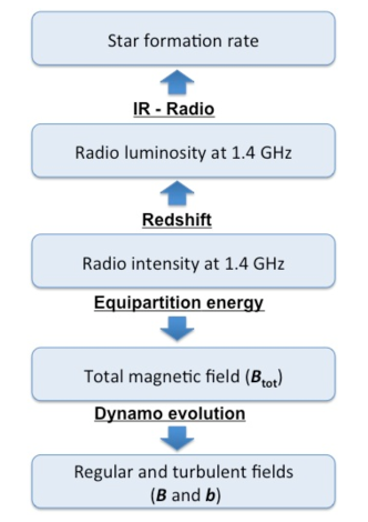
Figure 1: The diagram shows the link between SFR and magnetic field strength in a star-forming galaxy.

Here, we derive the link between the SFR and the amplitude of the total magnetic field. Bell (2003) used radio and IR luminosities of star-forming galaxies to calibrate the radio-derived SFRs. He showed that IR emission is a good indicator of the star formation in luminous galaxies, while in galaxies fainter by two orders of magnitude the IR emission traces a small fraction of the star formation. Because of the tight radio–IR correlation, this implies that the radio synchrotron emission is also suppressed in low-luminosity galaxies, compared to brighter galaxies which already has been observed in nearby spiral galaxies (Dumke et al. 2000; Chyży et al. 2007) and in dwarf galaxies (Klein 1991). This is taken into account in deriving the relation between the average SFR (in $M_{\odot}$ yr^-1) and the rest-frame radio luminosity at 1.4 GHz (see Bell 2003, Eq. (6)):

$$\mbox{SFR(radio)}=$$ (27)

$$=\left\{\begin{array}[]{cc}5.52\times 10^{-22}L_{1.4},&\mbox{if }L_{1.4}>L_{c}\\ \\ \displaystyle\frac{5.52\times 10^{-22}L_{1.4}}{0.1+0.9(L_{1.4}/L_{c})^{0.3}},&\mbox{if }L_{1.4}\leq L_{c},\\ \end{array}\right.$$

where $L_{c}=6.4\times 10^{21}$ W Hz^-1.

From the observed radio intensity of a galaxy one can estimate the radio luminosity and hence the star formation rate from Eq. (27). On the other hand, the radio intensity can be used to estimate the total magnetic field strength (Beck & Krause 2005) under the assumption of the equipartition between the energies of the CRs and the total magnetic field. In turn, the regular and turbulent magnetic-field amplitudes can be estimated from the total field strength (Eqs. (8-11)) using the timescale of amplification of the regular fields of the dynamo-evolution model (Arshakian et al. 2009). The scheme presented in Fig. 1 demonstrates the link between the SFR and the amplitudes of the total magnetic field, regular and turbulent fields.

Table 1: Radio luminosities, total field strengths and star-formation rates (SFR) in nearby spiral galaxies

Source	Type	$i$	$D$	$S_{4.85}$	$L_{1.4}$	$B_{\rm tot}$	SFR(radio)	SFR (IR, H$\alpha$)	Ref.
		$(\degr)$	(Mpc)	(mJy)	(W Hz-1)	$\mu$G	$M_{\odot}\,\mbox{yr}^{-1}$	$M_{\odot}\,\mbox{yr}^{-1}$
IC 342	SAB(rs)cd	25	3.1	856	$2.5\times 10^{21}$	10	1.6	1.2	1
M 31	SA(s)b	76	0.7	1863	$2.7\times 10^{20}$	3	0.3	0.30	2
M 33	SA(s)cd	56	0.8	1539	$3.3\times 10^{20}$	7	0.36	0.45	3
M 51	SAbc	20	9.7	380	$1.1\times 10^{22}$	17	5.3	3.1	4
M 81	SA(s)ab	59	3.3	385	$1.2\times 10^{21}$	8	0.96	0.89	5
M 83	SAB(s)c	24	3.7	809	$3.4\times 10^{21}$	18	2.0	1.6	1
NGC 253	SAB(s)c	78	3.9	2707	$1.3\times 10^{22}$	35	6.2	6.3	1
NGC 891	SA(s)b? sp	88	9.6	286	$8.1\times 10^{21}$	6	3.9	3.3	1
NGC 3628	SAb pec sp	89	6.7	247	$3.4\times 10^{21}$	6	2.0	1.1	1
NGC 4565	SA(s)b? sp	86	12.5	54	$2.6\times 10^{21}$	7	1.7	1.3	1
NGC 4631	SB(s)d	85	7.5	476	$8.2\times 10^{21}$	6	4.0	2.1	1
NGC 5775	SAbc	81	26.7	94	$2.1\times 10^{22}$	8	10.	7.3	1
NGC 5907	Sc	87	11.0	72	$9.9\times 10^{20}$	4	2.0	1.3	1
NGC 6946	SAB(rs)cd	38	7.0	457	$6.8\times 10^{21}$	16	3.3	3.2	4

• The columns are: source name, morphological type of a galaxy, $i$ is the inclination (degrees), $D$ is the distance of a galaxy (Mpc), $S_{4.85}$ is the total flux density at 4.85 GHz, $B_{\rm t}$ is the total magnetic field strength, SFR is the star-formation rate estimated from the radio luminosity at 4.85 GHz, SFR (IR, H$\alpha$) is the star-formation rate estimated from IR or H$\alpha$ emission, and the last column is the references to the SFR (H$\alpha$, IR) values. The references to SFR are: 1: Young et al. (1989), 2: Tabatabaei & Berkhuijsen (2010), 3: Verley et al. (2009), 4: Leroy et al. (2008), 5: Gordon et al. (2004).

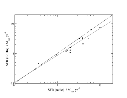
Figure 2: Comparison of SFRs of 14 nearby galaxies estimated from the radio emission at 1.4 GHz and the IR or H$\alpha$ emission. SFRs of nine galaxies (circles) are taken from Young et al. (1989) and five galaxies (triangles) from other papers (see Table 1). The dashed line represent the equality and the full line is the best linear fit to the data.

To test this scheme, we selected a sample of 14 nearby spiral galaxies with different inclinations and levels of star formation. For these galaxies, we integrated the observed radio intensities at 4.85 GHz and determined their flux densities $S_{4.85}$ as described in Stil et al. (2009) (see Table 1). Dividing by the area of integration gives the mean total intensities $I_{4.85}$ (mJy/beam) for these sources. We estimated the non-thermal intensities $I_{n4.85}$ accounting for a mean thermal fraction of 20 %. Further, from the 4.85 GHz flux density values $S_{4.85}$ we determined the radio luminosities $L_{4.85}$ and extrapolated these values to 1.4 GHz assuming a total spectral index of $\alpha=0.7$. The values for $L_{1.4}$ are also summarized in Table 1. We used Eq. (27) to calculate the values for the SFR(radio) from the radio luminosity at 1.4 GHz $L_{1.4}$ (see Table 1). To check the reliability of estimated SFR(radio), we compared them with the SFR values determined from the IR-emission (Young et al. 1989) for these galaxies, adopting Eq. (3) of Kennicutt (1998) or more recent values from the literature for special galaxies. The values determined from the radio emission and the other values correlate well for the 14 galaxies with $\rm{SFR(H\alpha,IR)}\propto\rm{SFR(radio)}^{0.88\pm 0.06}$ with a correlation coefficient of 0.97 (see Fig. 2). Good agreement between independent measurements suggests that the SFR can be reliably estimated from the radio luminosity at 1.4 GHz (Eq. (27)).

Using the $I_{n4.85}$ (see Table 1) and the pathlength through the emitting medium (assumed to be the diameter of the galaxy for edge-on galaxies), we estimated the total magnetic field strength $B_{\rm tot}$ under the assumption of the equipartition between the total energy of cosmic rays and that of the magnetic field (Beck & Krause 2005, their Eq. (3), using $\nu=4.85$ GHz and a synchrotron spectral index of $\alpha_{n}=0.8$). The knowledge of the SFR of a galaxy and its effective diameter (or the pathlength through the emitting medium) allows the $B_{\rm tot}$ to be estimated, and vise versa, the SFR can be derived from the $B_{\rm tot}$ and effective radius of a galaxy. In turn, independent measurements of a SFR and $B_{\rm tot}$ open a possibility to calculate the effective diameter of unresolved sources in deep radio surveys.

In the next section, we present simulations for one specific SFR because a variation of the SFR simply scales with $B_{\rm tot}$ in the case of an unchanged size of the galaxy during the evolution, as was assumed in this work.

5 Modeling the regular magnetic fields and radio emission properties

We perform modeling for a galaxy of the radius of 10 kpc inclined at an angle of $60^{\circ}$, and having a constant SFR=10 $M_{\sun}$ yr^-1 which corresponds to the radio luminosity $L_{1.4}=1.8\times 10^{22}$ W Hz^-1 at 1.4 GHz (Eq. (27)). The strength of the total magnetic field at the age $t\geq t_{\rm eql}=1.2$ Gyr is estimated to be $B_{\rm tot}(t)=6.9\,\mu$G, and the amplitudes of turbulent and regular fields are $b=6.2\,\mu$G and $B(t)=3.1\,\mu$G (Eqs. (10) and (11)).

We start the modeling of magnetic spots at the age of 0.8 Gyr (Sect. 3.2). We assume that the formation of $n=15$ magnetic spots of a scale length of 1 kpc in the disk (with a scale radius $8.3$ kpc and scale height $0.5$ kpc) are in place at $\approx 0.8$ Gyr after the disk formation. The amplitudes of the regular field of magnetic spots are distributed randomly around the mean coherent magnetic field strength $B(t=0.8)=0.6\,\mu\mathrm{G}$, within the range from $0.7B(t=0.8)$ to $1.3B(t=0.8)$, and coherent fields in the spots are oriented within the pitch angles $20^{\circ}\pm 5^{\circ}$ or $\pi+(20^{\circ}\pm 5^{\circ})$ with equal probability.

Table 2: The amplitudes of regular and turbulent fields, radial and azimuthal coherence scales simulated for different ages of a disk galaxy with inclination of $60^{\circ}$, scale radius of $R=10$ kpc, and SFR=10 $M_{\sun}$ yr^-1.

$t^{\mathrm{a}}$	$B$	$b$	$l_{r}$	$l_{\phi}$	$z^{\mathrm{b}}$	$\nu_{\rm z}^{\mathrm{c}}$
(Gyr)	$(\mu$G)	($\mu$G)	(kpc)	(kpc)		(MHz)
0	0.02	6.2	0.1	0.1	10	1650
0.8	0.6	6.2	1.0	2.9	4.7	855
1.3	3.1	6.2	1.6	4.5	3.6	690
2	3.1	6.2	2.5	6.8	2.5	525
3	3.1	6.2	3.6	10.	1.9	435
5	3.1	6.2	6.0	16.5	1.1	315
13	3.1	6.2	15.4	42.4	0.0	150

• $t$ is the age of a galaxy after the disk formation epoch assumed to occur at $z=10$.

• $z$ is the redshift of a galaxy calculated for a flat cosmology model ($\Omega_{\Lambda}+\Omega_{m}=1$) with $\Omega_{m}=0.3$ and $H_{0}=70$ km s^-1 Mpc^-1.

• $\nu_{\rm z}$ is the rest frame frequency which is detected at 150 MHz ($\lambda=2$ m) in the frame of the observer.

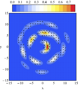
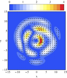
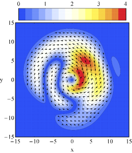
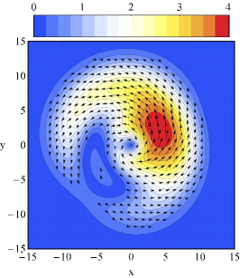
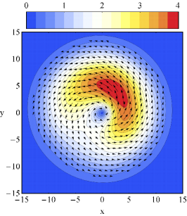
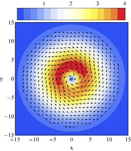
Figure 3: Simualtions in the framework of the SKA Design Studies (SKADS): the evolution of regular magnetic fields in the disk of a galaxy seen face-on (the frame size is 20 kpc$\times$20 kpc). The amplitude and ordering scale of the regular fields are estimated at 0.8 Gyr after the disk formation epoch ($\sim 1.3$ $\mu$G and 1 kpc), 1.3 Gyr ($\sim 3.1$ $\mu$G and 1.6 kpc), 2 Gyr ($3.1$ $\mu$G and 2.5 kpc), 3 Gyr ($\sim 1.5$ $\mu$G and 7 kpc), 5 Gyr ($\sim 3.1$ $\mu$G and 6 kpc), and after 13 Gyr ($\sim 3.1$ $\mu$G and 15.4 kpc). The color bar represents the amplitude of the regular field in units of $\mu$G.

Modeling the regular fields for an undisturbed (without a major merger) Milky-Way type galaxy (Fig. 3) show that the development of spotty structures with a coherence length of $\sim 1.5$ kpc is clearly visible during $\la 1.3$ Gyr after the disk formation. During the second Gyr the spotty patterns develop to prolonged structures of magnetic fields with a coherence length of $\sim 2.5$ kpc with few reversals of the field. After $\sim 5$ Gyr the reversals disappear and the coherence scale of the regular field reaches $\sim 6$ kpc. The fully coherent field is developed in $\sim 5$ Gyr while the asymmetry of the magnetic field strength remains longer.

Simulations of the total intensity, polarization and Faraday depth (see Appendix A for a mathematical description of equations) in the rest frame of a galaxy at 5 GHz after 0.8 Gyr, 2 Gyr, 3 Gyr, and 13 Gyr of disk formation are shown in Fig. 4. The symmetric structure in total intensity at the age of 0.8 Gyr (Fig. 4; first row) is due to strong turbulent field compared to the regular field (see Table 2). Smooth and weak polarized intensity and small Faraday rotation with no large-scale patterns are the result of a small ordering scale and small amplitude of the regular field at this age. At the age of 2 Gyr, the regular field has a coherence scale of $\sim 2.5$ kpc and few reversals, reaches the equipartition level and becomes comparable with the strength of the turbulent field ($B\approx b/2$). These changes are manifested by appearance of polarization patterns and asymmetric, inhomogeneous RM structures (Fig. 4; second row). After 13 Gyr, the regular field has no reversals and is coherent at the size of a galaxy (Fig. 4; third row). The polarization map looks symmetric with notable depolarization along the major axis, and the RM structure is smooth and asymmetric. Note that the intensity units in Fig. 4 have to be scaled via SFR (or total radio luminosity; see Sect. 4).

Simulations in the rest frame of the star-forming galaxy at 150 MHz are shown in Fig. 5. The main difference between the 5 GHz and 150 MHz maps is the effect of Faraday depolarization which becomes stronger at low radio frequencies. Depolarization along the major axis of a galaxy is stronger at large ages when the regular field becomes stronger and more ordered. The depolarization shapes the elongated polarized structure aligned near the minor axis of a galaxy (Fig. 5) which is clearly visible at 13 Gyr after the disk formation.

We also simulate the total intensity, polarization and Faraday depth in the rest frame of the observer at $\nu_{\rm obs}=150$ MHz (Fig. 6) taking into account the frequency shift of a galaxy at a redshift $z$ (see Appendix A for details). For more distant galaxies the synchrotron intensity, depolarization effect, and the regular magnetic field become weaker. The latter two effects lead to the small “observed” Faraday rotations at high redshifts (Fig. 6). The observed intensity at 150 MHz is emitted at high frequencies at high redshifts (Table 2).

Figure 4: The rest frame simulations of the total intensity (left panel), polarization (middle panel), and Faraday rotation (right panel) at 5 GHz for a galaxy with an inclination angle of $60\degr$, turbulent (6.2 $\mu$G) and regular (from 1.3 $\mu$G to 3.1 $\mu$G, see Table 2) magnetic fields, and star-formation rate of 10 $M_{\sun}$ yr^-1 are shown for 0.8 Gyr, 2 Gyr, 3 Gyr, and 13 Gyr after disk formation. The frame units are given in kpc. The color bars in the first and second columns (total and polarized intensity) are given given in arbitrary units. The color bar of the third column (Faraday rotation measure) is given in units of rad m^-2.

Figure 5: The rest frame simulations of polarization (left panel) and Faraday rotation (right panel) at 150 MHz, otherwise as in Fig. 4.

Figure 6: Simulations of the observed polarization (left panel) and Faraday rotation (right panel) at 150 MHz, otherwise as in Fig. 4.

6 Discussion and conclusions

The evolution of large-scale magnetic fields in galaxies has not been investigated in detail so far. Dynamo theory predicts the generation of large-scale coherent field patterns (“modes”), but the timescale of this process is comparable to that of the galaxy age (Sect. 2.2). Many galaxies are expected not to host fully coherent fields at the present epoch, especially those which suffered from major mergers or interactions with other galaxies.

Gissinger et al. (2009) presented the first global numerical simulation of a dynamo including superbubbles generated by SNRs, but without explicit inclusion of the alpha-effect (no mean-field assumption). The generated spiral field is strong and of quadrupolar symmetry, confirming the mean-field results, and it resembles the ”spotty” field injection.

Kinematical simulations of the field evolution in spiral galaxies without feedback to the gas flow, but excluding dynamo action (von Linden et al. 1998) revealed large-scale field structures which are partly oriented along the spiral arms, but also features of regular fields in the interarm regions which rapidly change their structure within one rotation of the galaxy and hence do not lead to a stable pattern. Presently it is unknown whether feedback of the field onto the gas flow may stabilize the field pattern.

The first global galactic-scale MHD simulation of a CR-driven dynamo with 100 pc resolution was performed by Hanasz et al. (2009) in which the cosmic rays are produced in randomly occurring supernova remnants. The timescales for amplification and ordering of the magnetic filed in their model are consistent with the dynamo timescales estimtated by Arshakian et al. (2009). This gives some confidence that the dynamo model correctly describes the overall properties of field evolution, especially as the simulations by Hanasz et al. (2009) also show “spotty” magnetic structures during the evolution from randomly spread seed fields to large-scale spiral structures. Even the ratio $h/R$ regulates itself in the CR–MHD simulations to a value near 0.1 which we assumed in the dynamo models (Hanasz, private communication).

Spiral arms and self gravity of the gas need to be included in future improvements of the model. The inclusion of shock fronts from supernova remnants will need higher spatial resolution. Furthermore, the effects of the SFR on the strength of the amplification and saturation of the regular magnetic field has still to be included into the model. As the SFR decreases with decreasing redshift and depends on merger rate, this may also influence the evolution of the magnetic field in evolving galaxies.

Predictions of the model. Comparison of our predictions with observations has to be restricted to spiral galaxies with thin disks and to high-frequency observations. Also, comparison is still restricted to nearby galaxies which can be resolved with the limited sensitivity of present-day telescopes. Among the existing observations, we could find spiral galaxies with well-developed large-scale spiral (axisymmetric) magnetic field structures, like in M 31 (Beck 1982; Berkhuijsen et al. 2003), IC 342 (Krause et al. 1989) and NGC 6946 (Beck 2007), as visible in polarized intensity and Faraday rotation similar to the last row in Fig. 4. All three galaxies are large with an exponential scale radius of about 5 kpc. Hence, according to Arshakian et al. (2009) it should have taken about 9 Gyr for these galaxies to coherently order the regular field structure over the entire disk (twice scale radius). This indicates that they did not suffer any major merger during this period. Indeed, NGC 6946 and IC 342 are isolated galaxies without any known companion and without any signs of major tidal distortions.

Observations of M 51 showed, however, that even if a large-scale spiral magnetic field is present in the galaxy’s disk and apparent in polarized intensity, it is hidden in the map of Faraday rotation (Fletcher et al. 2010) and looks much more patchy than that in row 3 of Fig. 4. This may be due to an additional magnetic field component, probably an isotropic turbulent magnetic field with scales of the longer axis between 400 pc to 1 kpc. Such a field has been found in M 51 (Fletcher et al. 2010) and in the barred galaxy NGC 1097 (Beck et al. 2005), but was not included into our simulations shown in Fig. 4 and Fig. 5. This component may be produced by strong shearing gas motions or compressions. It may also form loops perpendicular to the galaxy’s disk due to the Parker instability.

A prediction of our model is that interacting and merging galaxies should reveal complicated field patterns. The nearby and best studies case of strongly interacting/merging galaxies is the Antennae galaxy pair NGC 4038/39 observed in total and polarized radio emission by Chyży & Beck (2004). A huge polarized ridge in the northeast is probably the result of shearing flows. Another highly polarized region between the two galaxies marks the location of strongly compressed fields. The spiral field pattern of the galaxy in the northwest is still clearly visible. This galaxy is still in the phase before total field disruption and cannot be compared with our simulations.

A survey of polarized emission from galaxies in the Virgo cluster by Weżgowiec et al. (2007) and Weżgowiec et al. (2010) revealed signs of compression or shear in almost all galaxies, but the Faraday rotation data are still of insufficient quality to detect any delay in the formation of coherent fields.

Another prediction from our model, that small galaxies build up their large-scale field faster than large galaxies, also cannot be observationally confirmed with the existing data from nearby spiral galaxies. We need a sample of galaxies without massive density waves and without bars where the dynamo-generated field dominates over anisotropic fields. Furthermore, galaxies with strong signs of tidal interactions have to be excluded. A comparison with observations of dwarf and irregular galaxies fails because they do not fulfill the “thin-disk criteria” ($h/R<0.1$) discussed in Sect. 3.5.

Forthcoming observations of a large sample of spiral galaxies with high resolution and high sensitivity and of distant galaxies in early stages of the evolution with the SKA and its precursors should be able to test our scenario (Beck 2009).

Limitations of the model. Lacking a realistic MHD model of evolving galaxies, we tried in this paper to describe the evolution of large-scale fields by simple interpolation between the stages about which we believe to have some knowledge: the epoch of field seeding and the present epoch. This approach provided templates for radio maps in total and polarized intensity and in Faraday rotation measures, as part of the simulations for the SKA Design Studies (SKADS).

In Arshakian et al. (2009), we assumed that the “quasi-spherical” mean-field dynamo amplified the regular field and increased the coherence scale in radial direction, while the “disk” mean-field dynamo was effective in thin-disk galaxies. We note that the simulations of the “disk” mean-field dynamo described in the previous section cannot be performed for dwarf and irregular galaxies.

Another limitation of simulations comes from the fact that the strength of the cosmic microwave background energy density increases with increasing redshift, so that the synchrotron emission of star-forming galaxies will be quickly suppressed by inverse Compton losses off the cosmic microwave background at redshifts $z>3$ (Murphy 2009). In this paper, we do not account for this effect, but our simulations should be realistic for star-forming galaxies up to $z\approx 3$.

High SFR causes high velocity turbulence of the ionized gas in starburst galaxies, e.g. by a major merger of gas-rich galaxies. If SFR is higher than or equal to 20 $M_{\sun}$ yr^-1, the mean-field dynamo will be suppressed (Arshakian et al. 2009). Hence, our simulations are valid only for disk galaxies with ${\rm SFR}\la 20$ $M_{\sun}$ yr^-1.

In reality, the magnetic field evolution in first galaxies can be affected by various effects which are not accounted in our simple model. In particular, galactic winds (e.g. Moss et al. 2010), turbulent pumping (e.g. Brandenburg et al. 1995), and the multiscale nature of the interstellar medium (Mantere et al. 2010) can substantially affect the dynamo and result in a phenomenology which observably differs from predictions of our scenario. Future observations with SKA and its forthcoming pathfinders will be crucial to detect the difference with our simplified model and prove the importance of additional effects.

Furthermore, our simulations assume that the field structure in the halo is the same as in the disk and do not take into account the X-shaped halo fields observed around edge-on galaxies (Krause 2009). When observing mildly inclined galaxies at low frequencies, the polarized emission from the disk is mostly depolarized and the halo may dominate. In this case, our results for polarized and Faraday rotation images shown in Fig. 5 may change significantly. This can be tested by sensitive observations of edge-on galaxies at sufficiently high frequencies to avoid Faraday depolarization.

In summary, we link the SFR and amplitudes of the regular and turbulent fields in disk galaxies, further develop an evolutionary model for magnetic fields in isolated star-forming disk galaxies and performed modeling of the evolving galaxy. The amplitude of the initial “spotty” structure of regular fields (generated at the epoch of disk formation) is amplified by means of mean-field dynamo to the equipartition level in a few Gyr and remains at this level up to the present time. The ordering and azimuthal scales of initial magnetic spots increase with the age of a galaxy stretching the initial field in both directions. For the proposed model, we simulate the total intensity, polarization and Faraday rotation for the MW-type galaxy at different frequencies (from 150 MHz to 5 GHz) observable with the SKA and its precursors. A number of predictions such as the patchy structure and field reversals of regular fields, patchy Faraday rotations in galaxies younger than few Gyrs, smaller ordering scale in young galaxies, polarization patterns at 5 GHz and asymmetric structure at 150 MHz in older galaxies because of stronger depolarization, and the complicated field patterns in interacting and merging (minor and major) galaxies can be tested with the future radio telescopes.

Appendix A Equations for a total and polarized intensities, and Faraday rotation

The polarized signal passes a distance $w^{\prime}$ in the direction of the line-of-sight through a magneto-ionic medium of the galaxy inclined at an angle $i$. Then the Faraday rotation (in units of rad m^-2), polarization angle, and total intensity in the coordinate system inclined at an angle $i$ $(x,y^{\prime}=y\cos i,w^{\prime}=w\cos i)$ are

$$RM(x,y^{\prime},w^{\prime})=810\int_{-\infty}^{w^{\prime}}B_{\parallel}(\vec{r})n_{\rm{e}}(\vec{r})ds,$$ (28)

$$\chi(x,y^{\prime},w^{\prime},\lambda,z)=\chi_{0}(x,y^{\prime},w^{\prime})+$$ (29)

$$\left(\frac{\lambda}{1+z}\right)^{2}RM(x,y^{\prime},w^{\prime}),$$

and

$$I(x,y^{\prime},\lambda,z)=\left(\frac{\lambda}{1+z}\right)^{\alpha}\int_{-\infty}^{\infty}n_{c}(\vec{r})|B_{\bot}(\vec{r})|^{1+\alpha}ds,$$ (30)

where $B$ is the magnetic field strength measured in $\mu$G, $n_{\rm{e}}$ in cm^-3, $ds$ and $w^{\prime}$ in kpc, $\chi_{0}$ is the intrinsic magnetic field orientation (from the magnetic field model), $\lambda$ is the observed wavelength (in meters), $z$ is the redshift of a galaxy, $\alpha$ is the synchrotron spectral index ($\alpha=0.8$). The equations for Stokes parameters, $Q$ and $U$, are given by

$$Q(x,y^{\prime},\lambda,z)=$$ (31)

$$p_{i}\left(\frac{\lambda}{1+z}\right)^{\alpha}\int_{-\infty}^{+\infty}n_{c}(\vec{r})|B_{\bot}(\vec{r})|^{1+\alpha}\cos(2\chi)ds,$$

$$U(x,y^{\prime},\lambda,z)=$$ (32)

$$p_{i}\left(\frac{\lambda}{1+z}\right)^{\alpha}\int_{-\infty}^{+\infty}n_{c}(\vec{r})|B_{\bot}(\vec{r})|^{1+\alpha}\sin(2\chi)ds,$$

where $p_{i}=0.73$ is the intrinsic maximum polarization for synchrotron emission (for $\alpha=0.8$) in regular magnetic fields. Then, the “observed” polarization intensity

$$PI(x,y^{\prime},\lambda)=\sqrt{Q(x,y^{\prime},\lambda)^{2}+U(x,y^{\prime},\lambda)^{2}},$$ (33)

$$\chi_{\rm obs}(x,y^{\prime},\lambda)=\frac{1}{2}\arctan\frac{U(x,y^{\prime},\lambda)}{Q(x,y^{\prime},\lambda)},$$ (34)

and the “observed” RM is

$$RM_{\rm obs}(x,y^{\prime},\lambda)=\frac{\partial\chi(x,y^{\prime},\lambda^{2})}{\partial\lambda^{2}}.$$ (35)