Modelling the near-IR spectra of Jupiter using line-by-line methods

Abstract

We have obtained long-slit, infrared spectra of Jupiter with the Anglo Australian Telescope in the K and H bands at a resolving power of 2260. Using a line-by-line, radiative transfer model with the latest, improved spectral line data for methane and ammonia, we derive a model of the zonal characteristics in the atmosphere of this giant planet. We fit our model to the spectra of the zones and belts visible at 2.1 $\mu$m using different distributions of cloud opacities. The modeled spectra for each region match observations remarkably well at K band and in low pressure regions at the H band. Our results for the upper deck cloud distribution are consistent with previous models (Banfield et al.1998) fitted to low resolution, grism spectra. The ability to obtain and model high resolution planetary spectra in order to search for weakly absorbing atmospheric constituents can provide better constraints on the chemical composition of planetary atmospheres.

1 Introduction

The infrared spectrum of Jupiter is dominated by absorption features due to methane (CH₄) as well as other gases such as ammonia (NH₃) and collision induced absorption due to H₂ and He. Methane, however, has a very complex rovibrational spectrum and the available spectrum line data are limited. Many models for Jupiter’s spectrum have therefore been based on low resolution absorption coefficients or k-distribution data, rather than on line-by-line techniques. For example Strong et al. (1993) and Irwin et al. (2005) have presented k-distribution models for methane absorption at a resolution of 10 cm^-1, and Irwin et al. (1999) have presented similar data for ammonia. Using data such as this it is possible to model spectra at relatively low resolution such as those from Galileo-NIMS. However, many infrared spectrographs on ground-based telescopes can provide much higher spectral resolution. Recently there have been significant improvements in the available spectral line data for methane and ammonia (Albert et al. 2009; Rothman et al. 2009; Yurchenko et al. 2009; Nikitin et al. 2010; Wang et al. 2010).

In this paper we present a set of observations of the spectrum of Jupiter at a spectral resolution of $\sim$2260 and investigate our ability to model this data using line-by-line methods. We use the radiative transfer model VSTAR (Versatile Software for Transfer of Atmospheric Radiation), which is specifically designed for this purpose (Bailey 2006). It derives radiative transfer solutions for specified wavelength ranges in the transmission, emission or reflection spectrum of a planet. This software is designed to be extremely versatile in the range of atmospheres it can be applied to. In the past we have used it for the atmospheres of Earth and Venus (Bailey, Simpson & Crisp 2007; Bailey et al. 2008; Bailey 2009) and recent additions to the system allow it to be used for the atmospheres of solar-system planets, exoplanets, brown dwarfs and cool stars.

Methane is an important absorber, not just in Jupiter and the other solar system giant planets, but also in brown-dwarfs (the presence of methane absorption is the defining characteristic of a T-dwarf) and is likely to be important in many exoplanets. It has been reported in the spectra of the transiting exoplanets (Swain et al. 2008, 2009). While hot methane presents additional issues compared with the cool methane spectra required for Jupiter (e.g. Borysov et al. 2002) the problem of accurately modelling the methane absorption spectrum is common to a full understanding of all these objects. Thus Jupiter can be considered a test object for our future ability to model the spectra of extrasolar planets, as well as an interesting object in its own right.

Despite decades of research dedicated to understanding the structure and composition of Jupiter’s atmosphere, unanswered questions remain about the detailed distribution and transport of gases over the surface of the most massive planet of the Solar system. The wealth of data across its optical and infrared spectrum from ground-based telescopes (e.g. Clark & McCord 1979; Karkoschka 1994), Pioneer 10 (Tomasko et al. 1978), Voyager (Conrath & Gierasch 1986), Galileo (Carlson et al. 1996) and the Cassini spacecraft (Kunde et al. 2004; Bellucci et al. 2004) provided direct measurements of physical properties at different heights of the atmosphere, which can be used to constrain input parameters in models. Spectral information is used not only to derive the atomic and molecular abundances of the atmosphere given the physical properties such as temperature and pressure at different heights, but also to study the distribution of aerosols and clouds, and dynamic characteristics, which include wind and temperature patterns due to global weather effects.

Jupiter is covered with permanent layers of clouds, which are arranged into longitudinal, relatively stable regions determined by atmospheric circulation. The bright and dark bands are called zones and belts respectively, which are understood to correspond to up- and down-welling of gas in the convective flow of the atmosphere. The most abundant constituents of Jupiter’s atmosphere are hydrogen, helium, methane and ammonia. Direct measurements of the scattering properties in Jupiter atmosphere taken with the Galileo Probe Nephelometer (Ragent et al. 1998) suggest that the dense clouds of condensates, mostly ammonia, form in the almost adiabatic troposphere above 1600 to 700 mb. In addition the thinner, stratospheric hazes, which contribute to the overall atmospheric opacity, have been detected at heights, which vary depending on the longitude of the planet. For example they appear elevated in the polar regions, where hydrocarbons, such as C₂H₆ and C₂H₂ are suggested to exist as a product of photochemical and auroral discharge processes (Pryor & Hord 1991). Another molecule considered in a composition of the stratosphere is photochemically produced N₂H₄ (Strobel 1983). The detailed composition of stratospheric haze remains uncertain due to limitations of currently available data. A comprehensive review of Jupiter’s cloud structure was presented by Irwin (1999).

The observations described in this paper are long slit spectra at relatively high resolving power (R = $\lambda/\Delta\lambda\sim$ 2260) in the H and K band (Table 1). The data were obtained with the Infrared Imager and Spectrograph 2 (IRIS2), (Tinney et al. 2004) at the Anglo-Australian 3.9 Telescope. The spectra were subdivided into latitudinal regions, that closely resemble the pattern of zones and belts visible in the acquisition image observed with CH₄ filter at 1.673 $\mu$m (Figure 1). The details of calibration technique are discussed in Section 2. We used the VSTAR package to develop models of the cloud structure for each region to best fit the observed spectra. In Section 3 we describe the VSTAR modeling strategy to achieve this goal, which includes the model parameters and the lists of spectral lines used for each constituent of the atmosphere. The derived cloud opacities at different latitudinal locations are presented in Section 7, and followed by discussion in Section 5.

2 Observations and Data Reduction

The images and the IRIS2 spectra of Jupiter were acquired on the 25th of May 2007 (Table 1). The long slit (7.7^′) was positioned across the meridian of the planet. The width of the slit is 1^′′, which is equivalent to 2.2 pixels on the detector. The spectra cover the H (1.62-1.8 $\mu$m) and K (2.0-2.4 $\mu$m) bands. The narrow-band image of the whole planet in CH₄ (Figure 1) shows the characteristic band cloud structure. The calibrated spectra were extracted and averaged over 11 regions denoted by names given in Table 2. The region selection was based on the reflectivity profile averaged across the slit over the section of the K band spectrum in the region of the collision induced H₂-H₂ absorption between 2.08 and 2.13 $\mu$m. The black horizontal lines overploted on the image in Figure 1 show the extent of each region.

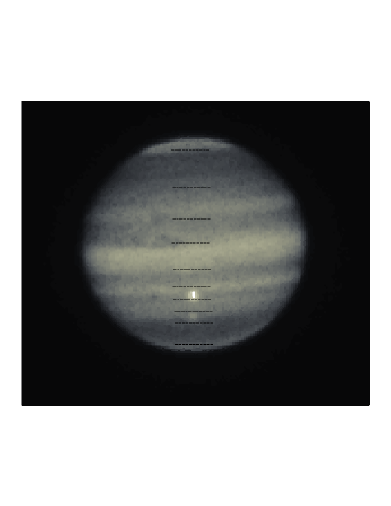
Figure 1: The narrow-band, acquisition image of Jupiter taken in the CH₄ absorption region at 1.673 $\mu$m shows a characteristic band structure of clouds in the atmosphere of the planet. The black lines mark the borders between regions, which correspond to zones and belts defined by the level of absorption visible at 2.1 $\mu$m through a 1^′′ slit positioned vertically at the centre of the planetary disk. All observed spectra are derived as the averages over the number of pixels comprising each zone or belt.

Data reduction was carried out using standard procedures of the Figaro package (Shortridge et al. 1995). The wavelength calibration was achieved by using a Xenon lamp. The spectra were divided by spectroscopic flat fields in order to remove the non-uniform response of the detector. The normalized flat-field images were formed by subtracting the image fully illuminated by a quartz calibration lamp and the dark image taken with the lamp switched off. Sky subtraction was achieved by taking four exposures with two spectra spatially offset in the same frame and subtracting two corresponding frames with offset spectra from each other.

Spectral curvature was removed by resampling the frames using correction derived from spectra of standard stars taken for each band. Bad pixels due to cosmic rays and known imperfections of the detector were corrected by interpolation between their neighbours.

We used standard stars, which were close in angular separation to the planet. They were chosen to match the solar spectral type as closely as possible. The Jupiter spectrum was divided by the standard star spectrum to remove both telluric absorptions and solar features. The resulting spectrum corresponds to the reflectance from the planet. Bailey, Simpson & Crisp (2007) have pointed out potential problems with using standard stars for removal of telluric absorption for planetary spectra. However, in the case of Jupiter the absorption features in the planet are due to different molecules from those in the terrestrial atmosphere spectrum and these problems are largely avoided.

A true level of intensity can be derived by converting a number of counts, $N^{c}$ in the spectra into the flux density derived from the calibrated flux density, F_st, of the standard star. We derive the radiance factor, I/F_Sun, where I is the reflected intensity of the planet and $\pi$F_Sun is the solar flux incident on the planet from:

$$\frac{I}{F_{Sun}}=\pi\frac{4D^{2}(N^{c}_{Jupiter})F_{st}}{\pi F_{Sun}(N^{c}_{st})(A_{slit})^{2}}$$ (1)

The size of the slit, A_slit is given in radians, and the distance of Jupiter, D from the Sun is measured in astronomical units. The flux in each region is then scaled by the number of pixels, it encompasses.

Table 1: Jupiter observations on the 25 May 2007

Band	Centre	Resolving power	Mean dispersion	Start (UT)	Integration Time	Total
	($\mu$m)		(nm/pixel)	(h)	(s)	(s)
H	1.637	2270	0.341	14:40	12	48
K	2.249	2250	0.442	14:58	45	180

The typical spectrum and our VSTAR model in the equatorial region of Jupiter are presented in Figure 2 in the wavelength range between 1.62 and 2.4 microns. As expected the methane absorption clearly dominates in this spectral range. The H₂-H₂, collision induced smooth absorption peaks at 2.12 $\mu$m, which appears to be very shallow in the polar region spectra. This reflects the contributions of increasingly slant paths through the atmosphere, which probe vertically higher regions with lower density of H₂.

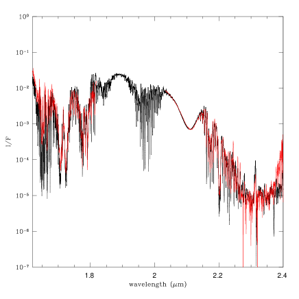
Figure 2: The observed spectrum (grey or red in the online version) of Jupiter’s equatorial region (EZ) at K and H band overlapped with the model (black), which also cover the region between 1.85 and 2 $\mu$m characterized by the strong H₂O absorption in the Earth’s atmosphere and thus it is difficult to observe from the Earth. The main discrepancy between the model and observations appears at the low absorption region below 1.65 $\mu$m, which probes atmosphere levels below 1 bar. In addition we find typically larger mismatch in intensity of the methane absorption bands at H band than in K band, which is discussed in Section 7.

The moon, Europa was transiting in front of the planet during the observations and its reflected light was present in the slit while the spectra were taken. Its effect on the spectra of the Southern Equatorial Zone (SEZ) and Southern Belt (SB) is clearly be visible in Figure 7 showing the increased reflectivity in the regions of the largest methane absorption. Europa is thought to have the large amount of pure water ice on its surface (see the spectra in Calvin et al. (1995)). The highly reflective shoulders of water bands observed in the spectra around 1.8 and 2.2 $\mu$m contribute to the combined high albedo of the planet and the moon in the regions where otherwise the planetary methane absorption is the highest.

Table 2: List of selected regions of Jupiter

	Region
1	North Pole (NP)
2	Northern Upper Belt (NUB)
3	Northern Zone (NZ)
4	Northern Equatorial Belt (NEB)
5	Equatorial Zone (EZ)
6	Equatorial Belt (EB)
7	Southern Equatorial Zone (SEZ) a
8	Southern Belt (SB) a
9	Southern Zone (SZ) b
10	Southern Upper Belt (SUB)
11	South Pole (SP)

^aThese spectra are affected by a contribution of light reflected by Europa. ^bA spectrum of the atmospheric region with a bright ’white’ spot.

3 The VSTAR modeling procedure

The Versatile Software for Transfer of Atmospheric Radiation (VSTAR) is a modular code written in Fortran, which solves the line-by-line, radiative transfer problem for light in a stratified atmosphere with a defined chemical composition and a specified size distribution of cloud particles. The code is composed of several packages (MOD, LIN, RAY, PART and RT) which contain routines called by a user written program to build a specific atmospheric model.

The MOD package defines a two dimensional grid, which stores the values of parameters for the atmospheric layers in one dimension and the array of spectral points at which the model is calculated in the second dimension. The LIN package reads spectral lines from the line databases, calculate line profiles and sets the optical depth for each layer of the atmosphere. The RAY package calculates Rayleigh scattering optical depth for the atmospheric layers. The particle scattering from aerosols and clouds is calculated with a Mie scattering code (Mishchenko et al. 2002). The PART package allows up to 20 different scattering particle modes with different size distributions, refractive indices and vertical distributions to be included in the model. The workhorse of the VSTAR code is the RT package, which performs the radiative transfer solution for each layer of the atmosphere using the data set up by the previously described packages. Different radiative transfer solvers can be selected but for the purpose of this work we use DISORT, the discrete ordinate solver described in Stanmes et al. (1988).

We model Jupiter’s atmosphere using 36 vertical layers with specific physical properties given by pressure, temperature, as well as chemical composition expressed in terms of gas mixing ratios. The P-T profile of the planet’s atmosphere in the pressure range between 0.001-1 bar has been studied with infrared radiometry, radio occultations and direct sensing with the Galileo probe ASI experiment (Seiff et al. 1998). Most recent retrievals of atmospheric temperatures from the Cassini CIRS data published by Simon-Miller et al. (2006) show time-variable, zonal differences in P-T profiles, which are also present in the Voyager IRIS data. In the range of pressures probed with our model the strongest zonal variations are of the order of a few Kelvin in the upper troposhere.

In figure 4 we plot the averaged profile from Voyager radio occultation experiments (Lindal 1992), and the profile obtained from the Galileo probe descending into the 5-$\mu$m hot spot region in the north equatorial belt (Seiff et al. 1998). The notable differences in Voyager and Galileo profiles appear above about 300 mb in the upper troposphere, which is expected since both profiles were probing different locations on Jupiter surface at different times. The 5-$\mu$m hot spots are relatively dry, localized regions with a low level of cloud cover (Showman & Dowling 2000). We believe the Voyager occultation data are likely to be more robust in describing the average properties of zones and belts considered in our models. We tested the effects of changed temperature corresponding to the profile differences observed in Voyager ingress, egress occultations data and Galileo probe measurements for the Equatorial belt, Equatorial zone and the North polar region. The typical example of a difference between models with Voyager and Galileo derived P-T profiles is shown in Figure 4. The differences are highest in the spectral ranges corresponding to the tropospheric pressures. However they are of the order of magnitude lower than the typical residuals of our fits to data, which are dominated by the opacities of different vertical regions in the atmosphere.

Therefore for simplicity we used a single P-T profile to model zonal composition of the atmosphere based on the Voyager radio occultation observations (Lindal et al. 1981; Lindal 1992).

Figure 3: The observed spectrum of Jupiter’s equatorial region (EZ) at K and H band is shown with the difference between two models (in the lower panel) obtained with the Galileo Probe and the Voyager radio occultation P-T profiles,as presented in figure 4.

The chemistry of Jupiter’s atmosphere is complex and involves a large number of atomic and molecular species produced in photochemical processes (Atreya et al. 1997). Our model considers only the major components of the atmosphere, which influence the shape of the observed spectra in the near infrared region. The most abundant atmospheric gases are H₂ and He that produce smooth, collision-induced absorption features around 2.12 $\mu$m. The other molecules, which absorb in the infrared spectral region, are methane (CH₄) and ammonia (NH₃). Methane is the most important absorber in the H and K band spectra. The mixing ratio of CH₄ adopted in our model is $2.3\times 10^{-3}$, which is consistent with the latest in situ measurements with the Galileo Probe Mass Spectrometer (GPMS) (Wong et al. 2004). The mixing ratio of methane is relatively constant at pressures higher than 1 mbar (Moses et al. 2005).

Figure 4: Comparison between the temperature-pressure Voyager (solid line) and Galileo probe (dash line) profiles.

3.1 The Methane Spectrum

A tetrahedral molecule like methane has four vibrational modes, two bending modes described by quantum numbers $\nu_{1}$ and $\nu_{3}$ and two stretching modes $\nu_{2}$ and $\nu_{4}$, so that each vibrational level can be described by its four vibrational quantum numbers $(\nu_{1},\nu_{2},\nu_{3},\nu_{4})$. The frequencies of the two stretching modes are both about 1500 cm^-1 and the two bending modes both about 3000 cm^-1. These coincidences result in a complex series of interacting vibrational states repeating at intervals of $\sim$1500 cm^-1 known as polyads. Polyads are generally designated by P_n where n is the polyad number defined in terms of the vibrational quantum numbers by

$$n=2(\nu_{1}+\nu_{3})+\nu_{2}+\nu_{4}$$ (2)

P₀ denotes the ground state. The first polyad P₁ is also known as the Dyad since it contains the two vibrational levels $(0,1,0,0)$ and $(0,0,0,1)$. The P₂ polyad (or Pentad) contains 5 vibrational levels $(1,0,0,0)$, $(0,2,0,0)$, $(0,0,1,0)$, $(0,0,0,2)$ and $(0,1,0,1)$. Similarly P₃ is the Octad (8 levels) and P₄ is the Tetradecad (14 levels). The number of levels grows rapidly for higher polyad numbers and results in complex systems of interacting bands which are increasingly difficult to model as the polyad number grows.

A significant recent development is a new global analysis of the methane spectrum over the wavenumber range 0–4800 cm^-1 (levels up to the Octad) reported by Albert et al. (2009). The new model fits line positions and intensities much better than previous analyses of individual polyads (e.g. Hilico et al. 2001). The new model forms the basis of an improved set of methane line parameters included in the 2008 edition of the HITRAN database (Rothman et al. 2009). It provides a good model of the low temperature methane spectrum for wavelengths greater than about 2.1 $\mu$m.

However, at shorter wavelengths (higher polyads) HITRAN 2008 lists mostly empirical line parameters from Brown (2005). These are measured line intensities and positions at room temperature, and mostly lack quantum identifications and lower-state energies. The lack of a lower-state energy means that line intensities cannot be reliably determined for temperatures other than those of the original measurement. These lines are therefore not useful for modelling the spectra of the giant planets. However, some lines in the strongest part of the P₄ band system have empirically determined lower state energies derived from measuring the lines at two or more different temperatures. These lines, with data from Margolis et al. (1990) and Gao et al. (2009) cover the wavenumber range from 5500–6180 cm^-1.

For this work, we therefore constructed a methane line list as follows. We used line data from HITRAN 2008 for all wavenumbers up to 4800 cm^-1. We also used HITRAN 2008 for the region from 5500–5550 cm^-1, where empirical lower state energies are available. For the wavenumber range from 4700–5500 cm^-1, we used line parameters calculated using the Spherical Top Data System (STDS Wenger & Champion 1998). This range overlaps slightly with the range from HITRAN, but the lines from HITRAN are all in the P₃ polyad system in this region, whereas the STDS lines are all from the P₄ polyad, so there is no duplication. While the STDS effective hamiltonian model for the Tetradecad region is a preliminary one and does not give line positions that accurately match data, it does provide an adequate description of the overall band shape, and provides the lower state energies that are missing from HITRAN in these regions. For the range 5550–6236 cm^-1 we used line data from Nikitin et al. (2010) supplemented with low temperature empirical data from Wang et al. (2010). We have not attempted to model wavelengths shorter than 1.6 $\mu$m. However, new empirical methane line data for these wavelength regions are starting to become available (Campargue et al. 2010a, b; Sciamma-O’Brien et al 2009), which may enable our modelling to be extended to shorter wavelengths.

The line width data provided in HITRAN are for broadening in air. Data on broadening of methane lines in the $\nu_{3}$ band in a variety of broadening gases by Pine (1992), and Pine & Gabard (2003) shows that line widths broadened by H₂ are about 2% higher than those broadened by N₂, those in O₂ are about 6% less, and those in He are about 35% lower. This suggests that line widths in an H₂/He atmosphere should be very similar to those in an N₂/O₂ atmosphere. We have therefore used the air broadening data from HITRAN to determine the line widths in this work. Where the line data are taken from sources without broadening parameters, we used the default line half width value of $\gamma$ = 0.06 cm^-1 atm^-1 and a temperature exponent N = 0.85 as recommended by Nikitin et al. (2010).

3.2 Other Absorbers

The atmospheric abundance of NH₃ at high pressures was measured directly with GPMS and from the attenuation of radio signal sent between the probe and orbiter (Folkner et al. 1998). The mixing ratio appears to decrease from 10^-4 at pressures above 2 bar to 10^-6 below 1 bar. Ammonia is known to exist in gaseous form and as condensed clouds in Jupiter’s troposphere up to pressures of 0.1 bar (Kunde et al. 1982), but it is rapidly depleted in the stratosphere, due to UV photolysis.

The mixing ratios of NH₃ adopted in our model are constant ($2\times 10^{-4}$) in layers between 1 and 0.5 bar. They decrease to $2\times 10^{-7}$ at the 100 mbar along the saturated vapour pressure curve. The resulting profile is consistent with mixing ratios derived from the radio data in Sault et al. (2004) above 0.5 bar. They note small differences between the Equatorial Zone and North Equatorial Belt profiles, which we also tested in our models. As a result we observe changes in the absorption spectrum between 1.8 and 2 $\mu$m, where the $\nu_{1}+\nu_{4}$ and $\nu_{3}+\nu_{4}$ bands of NH₃ are present. We found that removing ammonia from the upper atmosphere ($<0.5$ bar), which is most likely the case in down-welling regions, like belts and hot spots, does not have a significant effect on the K and H band spectra which are dominated by CH₄ absorption.

Absorption of ammonia was derived from the new list of Yurchenko et al. (2009) which contains over 3 million lines and is considerably more complete than the line parameters in HITRAN 2008, including improved shorter wavelength coverage.

The bulk of Jupiter’s atmosphere consists of H₂ and He. Rotovibrational absorption bands due to collisions between pairs of H₂-H₂ and H₂-He exist in the near infrared region under consideration, where they form a smooth feature centred around 2.1$\mu$m. Our model includes absorption coefficients for H₂-H₂ and H₂-He pairs at low temperatures, derived by Borysow (2002) and Borysow et al. (1989) respectively.

It is worth noting that the 2.1$\mu$m collision induced absorption (CIA) depends also on the para-ortho ratio of hydrogen spin isomers in the atmosphere of Jupiter. Our current models assume the equilibrium ratio at all temperatures. The Voyager IRIS data was used by Conrath et al. (1998) to demonstrate that the distribution of that ratio varies in the different zonal and vertical regions of the planet. The deviation from so called ’normal’, 1:3, room temperature, equilibrium value is relatively low for Jupiter, but it can produce a noticable effect on the shape of the 2.1$\mu$m feature in the spectrum.

Our intention is to extend the capability of the VSTAR package in the near future to allow differences of the para-ortho H ratio as a function of atmospheric height, which will allow more accurate fit of the CIA absorption in atmospheres of cold giant planets, where the observed para-ortho ratios deviate even further from the normal value.

3.3 Scattering

In our model Rayleigh scattering from molecules and particle scattering from aerosols suspended in the atmosphere was considered. The Rayleigh scattering at wavelengths above 1 $\mu$m is much reduced in comparison with scattering from clouds. The Rayleigh cross sections (Liou 2002) were calculated for scattering in a mixture of H₂ and He, the dominant components of the atmosphere.

The vertical structure of aerosols in Jupiter’s atmosphere, derived directly from Galileo observations was surprisingly different from theoretical predictions (Atreya et al. 1997), which can be attributed to the unique region of the Probe entry. The Galileo Solid State Imager (SSI) observations covered more extended regions over belts and zones as described in Banfield et al. (1998). The SSI images taken close to the limb of Jupiter gave good information about the cloud opacity in the stratosphere.

Banfield et al. (1998) used a retrieval technique (Banfield et al. 1996) to obtain the scatterer density with altitude in the same spectral region as our observations. The upper troposphere between 700 and 100 mbar, and stratosphere at pressures lower than 100 mbar defined by Banfield et al. are within the spectral sensitivity of the H and K bands. The results of the Banfield et al. retrieval of particle distribution from the Galileo imaging suggest two enhancements in cloud opacity corresponding to the upper haze between 200 up to 20 mbar, and at the base of the tropospheric, condensation cloud at about 850 mbar. In equatorial regions, the upper haze is elevated to even lower pressures.

The layer of smaller particles is believed to form a relatively uniform top of the tropospheric cloud, which contains larger particles of presumably NH₃ ice and other condensates. Observations of limb darkening in the ultraviolet (Tomasko et al. 1986) constrain the size of the stratospheric haze to between 0.2 and 0.5 $\mu$m. To model the clouds we chose a simple two-component distribution of mean particle sizes, 0.3$\mu$m for the stratosphere and the conservative value of 1.3 $\mu$m size species for the upper tropospheric cloud. The combined observations from NIMS and NIR identify the lower tropospheric cloud as a mixture of two types of particles with 50 and 0.45 $\mu$m size, consistent with NH₄SH molecule (Irwin 1999). The upper troposphere, which our data is sensitive to, is believed to consists of 0.75 $\mu$m size ammonia particles.

The scattering properties of these clouds are calculated using Lorentz-Mie theory for a power-law particle size distribution. The code calculates the asymmetry factor, extinction and scattering coefficient, which are required in the radiative transfer calculations. The refractive index of the cloud particles is approximated by the refractive index of ammonia ice given by Martonchik et al. (1984) for a wide range of wavelengths.

In our model the vertical structure of the particle clouds is varied through the input list of optical depths for each layer of the atmosphere at the reference wavelength of 1.5 $\mu$m. Finally the boundary conditions for the model are given. Solar illumination at a given beam angle is provided using data from Kurucz (2009) and a non-reflecting surface is specified at the base of the atmosphere. The set of line data, particle properties and their distribution form inputs for the DISORT radiation transfer equation solver, which returns the fluxes and radiances at the top of the atmosphere for each wavelength specified in the grid. The models were calculated at a spectral resolution of 0.01 cm^-1, sufficient to resolve the spectral structure, and then convolved with an instrumental point spread function for comparison with the observed spectra.

4 Model of the bands in the atmosphere of Jupiter

To show the functionality of the VSTAR code, we used the most recent observational data described in the previous section, which provided the input parameters for characterisation of Jupiter’s atmosphere. We tested the sensitivity of our models to changes in these parameters and confirmed that spectral features are dominated by methane absorption with the addition of clouds above the 800 mbar level.

A simple model of the longitudinal belts and zones in the atmosphere of Jupiter was derived by manually varying the amount and vertical distribution of cloud opacity at different heights, while the chemical composition of the atmosphere was left constant across the surface of the planet. Since this is clearly not practical to explore full range of opacities at all levels of the atmosphere, we resorted to testing different combinations of opacities in the iterative way and fine-tuned them until a reasonable fit, with the smallest scatter in residual differences between spectra and models was achieved for both spectral bands H and K.

Figure 5: In the upper panels the observed spectra of the selected zones and belts in the K band (on the logarithmic intensity scale) are compared with the corresponding VSTAR models derived for these regions. In the lower panel the observed spectra in the H band are compared with the VSTAR models. The panels on the right (top and bottom) demonstrate the residuals obtained by taking the difference between the modelled spectra and corresponding data.

Figure 5 shows the line-by-line models for the selected bands and zones with a resolution that matches the observed spectra. Our models mirror most spectral features remarkably accurately considering that the average spectrum is a composite of sub-regions with possibly non-uniform cloud composition as evident in high resolution images from the Galileo SSI probes (Simon-Miller et al. 2001). We found that the most significant differences between the models and the data occurred in the equatorial zones, in spectral regions that correspond to the upper layers of the troposphere.

The most recognizable features of the K band spectrum are the H₂-H₂ collision-induced broad absorption centered at 2.11 $\mu$m and stronger absorption in the 2.2 to 2.4 $\mu$m region due to methane bands. The narrower CH₄ absorption features are due to the Q branches ($\Delta J=0$) of $\nu_{2}+\nu_{3}$ at 2.2 $\mu$m, $\nu_{3}+\nu_{4}$ at 2.32 $\mu$m and $\nu_{1}+\nu_{4}$ at 2.37 $\mu$m. The latter two bands are not always clearly visible in the observed spectra due to low signal-to-noise in the high methane absorption region and a decreased sensitivity at the edge of K band filter.

Spectra of the polar regions show the broad methane, and H₂-H₂ collision induced absorption much reduced as compared with the equatorial zones and belts. This can be understood by noting that the spectra of the polar regions sample relatively longer path-lengths through the higher layers of the atmosphere, which unlike the deep layers contribute little to the H₂-H₂ absorption.

Table 3: Total cloud optical depths in zones and belts

Particles	1.3$\mu$m		0.3$\mu$m
Zones	Extent	$\tau$	Extent	$\tau$
	(mb)		(mb)
NP	563-631	1.50	56-200	0.0100
			3-7	0.0030
NUB	316-562	0.52	125-200	0.0003
			25-40	0.0015
			7-9	0.0001
NZ	316-631	1.72	22-25	0.0010
NEB	355-751	5.70	25-35	0.0018
EZ	251-631	5.72	18-22	0.0023
EB	316-708	5.09	25-35	0.0070
SEZa	447-708	3.10	39-50	0.0720
SBa	355-708	6.06	141-251	$0.0188$
			40-50	0.0090
SZb	446-631	2.25	100-355	$0.0295$
			25-35	0.0060
			3-5	0.0010
SUB	316-751	1.29	141-316	0.0024
			25-40	0.0080
SP	251-708	2.20	22-251	0.0038
			2-4	0.0012

^aThe spectra affected by a contribution of light reflected by Europa, which boosts reflection in the otherwise most highly absorbing methane bands regions in K and H bands. This additional reflection was not included in the modelling. ^bA spectrum of the atmospheric region with a bright, ’white’ spot, which can be modelled as the relatively thick stratospheric cloud extending upwards to 100 mbar.

The models are constrained by a simultaneous fit of absorption levels for the broad and narrow band features of the spectra in both bands H and K. The lower panel of Figure 5 shows the spectra and models of the H band. The narrow spectral lines in the models tend to agree better with the observed spectrum than the broad shape and the intensity of absorption. We attribute this to the less accurate models of methane line parameters in this spectral region as discussed in section 3.1. The accuracy of the wavelength fit is limited mostly by the spectral calibration of the data, dominated by the correction of spectral curvature in the IRIS2 grism system. The wavelength of clearly identified lines in the data and models agrees within $5\times 10^{-4}\mu$m. Most discrepancies in models and observed spectra are due to the differences in intensity of a particular line or line series in methane absorption.

The Jupiter K band spectrum is defined by the opacities distributed between about 700 and 2 mbar. The shape of collision induced H₂-H₂ absorption, which samples deep layers of the atmosphere is highly sensitive to the cloud optical depth in the Jupiter’s troposphere, while the level of broad methane absorption beyond 2.2 $\mu$m varies dramatically in response to changes in the stratospheric cloud optical depth. The H band spectral region samples the higher levels of the troposphere.

Table 3 shows the total optical depths of the tropospheric (1.3 $\mu$m particles) and stratospheric aerosols (0.3 $\mu$m particles), which gave the best fit for each spectrum. All zones and belts show differences in the vertical distribution and the strength of opacity. Most notably the atmosphere appears to be relatively clear between 200 and 40 mbar in the northern and equatorial regions, which is consistent with conclusions in Banfield et al. (1998), who find a similar clearing around 100 mbar in their models in the same spectral region. We find that no trial models with added cloud opacity in this pressure range were able to reproduce the observed spectra.

We find that the clouds tend to lie deeper in belts than in zones. The tropospheric cloud seems to extend up to 250 mb in the equatorial region with the highest total opacity of the order of $\tau=5$, while the stratospheric haze is very thin with the opacities below $\tau\sim$ 0.005. Our models suggest that this haze may be slightly thicker in the southern hemisphere of the planet. However the SEZ and SB regions are affected by the spectrum of Europa, while the spectrum of the SZ zone may reflect a local cloud pattern.

The image of Jupiter (Figure 1) shows a rather large white spot in this region, which is subtended by a slit. The high resolution images taken by the New Horizons LEISA imager at 1.53 and 1.88 $\mu$m in February 2007 show similar weather features in the region of SZ and SUB. This spot is most likely a storm system such as the anticyclonic white oval modelled in Simon-Miller et al. (2001). They note that fresh material is upwelled in such high-pressure systems, which forms slightly higher clouds. Our model of the SZ white spot requires a relatively thick cloud at the 100-251 mb pressures with the small size particles, such as used for the stratospheric layers, which provided better fit to the observed spectra than any larger particles.

The zones clear of Europa light show higher stratospheric cloud opacities, which are distributed more thinly than clouds in nearby belts. The stratosphere in the high latitude northern (NUB) zone is more spread-out but relatively thin compared with the equatorial regions. The stratosphere above the southern upper (SUB) belt is also vertically extended, but in contrast to the NUB, has higher opacity. Previous models (West et al. 1986; Simon-Miller et al. 2001) suggested that downwelling of the haze in the belt regions could produce thinner cloud at high pressures. Our models show unambiguously increased opacity of high stratospheric layers in polar regions, which is consistent with the previous studies of Jupiter’s atmosphere (Pryor & Hord 1991).

Figure 6: The observed spectra, models and the difference between them (on the linear intensity scale) are shown for the northern and southern, high latitude zones (NZ and SZ) and belts (NUB and SUB). Although the spectra of the northen regions show typically stronger absorption visible in both H₂-H₂ feature and the wavelength region above 2.2 $\mu$m, this differences can be explained in terms of ’local’ weather effects as discussed in Section 7.

In Figure 6 the models of remaining regions are presented. Northern and southern zones (NZ and SZ) display a slightly different shape of the collisional absorption, which suggests the existence of more compressed, optically thicker tropospheric cloud in SZ than the cloud in the NZ. The SEZ and SB spectra (Figure 7) show the additional opacity due to Europa’s spectrum dominated by fine-grained water ice (Carlson et al. 1996). The effects of this opacity are clearly visible in the spectral region beyond 2.15 $\mu$m, which is sensitive to the highest atmospheric levels in our model.

Figure 7: The spectra of zones affected by opacity of Europa are shown compared with the simple models, which neglect the scattering contribution from this moon. The differences between spectra and models (bottom panels) show this clearly for spectral regions above 2.2$\mu$m .

5 Discussion

The line-by-line radiative transfer models for high resolution spectra from currently available ground-based instruments serve as an important test of the consistency in our understanding of the composition and processes that govern planetary atmospheres.

We achieved a good fit to the data assuming relatively simple physical structure and chemical composition of Jupiter’s atmosphere that was kept uniform across the whole surface of the planet. The real atmosphere is certainly more complex. Lacking a detailed P-T profile for each zone and belt we used a single profile of the atmosphere for all regions based on radio occultation observations (Lindal 1992). This seems justified despite small differences in atmospheric profiles observed by Voyager 1 infrared spectrometer (IRIS) and Cassini CIRS experiments (Simon-Miller et al. 2006) for different locations on the planet. It is argued, that because horizontal differences in observed brightness temperature are small, the larger deviations in observed brightness temperature are probably due to varied opacity in the clouds (West et al. 1986).

We also used a relatively simple representation of the chemical composition of the atmosphere, despite the fact that the abundances of gases in different regions of the atmosphere may vary with height due to evidently complex, planetary weather system. The upwelling in zones may cause the depletion of volatiles due to condensation and precipitation. In the down-well regions the mixing ratios of such volatiles may be increased in deeper levels of the atmosphere. While methane is well mixed within the vertical region of our sensitivity, there have been zonal differences in mixing ratios profiles of ammonia below 600 mbar suggested by Sault et al. (2004). Our models turned out to be not sensitive to these differences due to combined effect of the low NH₃ absorption in our spectral range and decreased sensitivity of our models to layers below $\sim 700$ mbar. We find that it is sufficient to consider only the major contributors to the spectral absorption at H and K bands: H₂, He, CH₄ and NH₃ and to modify the opacities of aerosols at different heights. However our systematically worse fits in equatorial zones may reflect the unrecognized complexity in these regions, which is not described in sufficient detail by the initial parameters of our model, such as P-T profile and mixing ratios of the chemical components.

The suggested constituents of clouds in the troposphere below 500 mbar are H₂O, NH₄SH and NH₃. Ammonia condensation occurs at the highest level at about 700 mbar at its saturation point. The actual condensation level can be lowered or lifted due to differences in the molar abundances of NH₃. West et al. (1986) suggested that the cloud needs to have a mixed composition of particles with sizes between 3 and 100 $\mu$m to explain high opacity observed at 45 $\mu$m. The larger particles are concentrated at the base of the cloud at pressures below our sensitivity limit. Consistently our models are most sensitive to changes in the particle sizes below 3 $\mu$m. We find that the tropospheric cloud in belt regions occurs at typically higher pressures compared to zones, which could be interpreted as the result of vigorous convective downwelling and upwelling process.

In contrast the stable haze of $\sim 1\mu$m-size particles, mixture of ammonia ices and residual chromophores responsible for the coloration of the clouds exists above the lower, convective troposphere. In the warmer temperatures there is no condensation expected and consequently no cloud formation. The origin of the stratospheric haze is thought to be due to photochemical processes.

This original picture of the layers above 700 mbar shown in West et al. (1986) was developed further by Banfield et al. (1998), whose model includes a clearing of the haze at about 100 mbar pressures. They explain it by the aerosol coagulation at this level of stratosphere, which is the cause of the increased, gravitational fallout of heavy particles. We observe such a clearing in models of most of the northern zones and belts of the planet. Above the clearing we find the optically thin haze of reflective particles with a predominantly lower sizes, than particles in the troposphere. This haze extends to the low pressures of 2 mbar in the polar regions. The chemical composition of the stratospheric haze is still debated. It is also no clear if the polar haze observed at lower pressures has the same composition as the equatorial stratosphere.

6 Summary

We have used the new, line-by-line, radiative transfer package, VSTAR, to model the near infrared spectra of Jupiter. The models were produced for regions with different absorption properties implied by varied cloud patterns in the atmosphere of the planet. With our improved database of methane absorption lines at low temperatures, we achieved a good fit to the spectra obtained with the AAT/IRIS2. We were able to reproduce conclusions suggested in previous studies about the atmospheric conditions at pressures below 1 bar, which probe the upper troposphere and stratosphere of the planet. We showed that ground-based spectroscopy with large telescopes can significantly enhance the results achieved from space. With continued improvements in methane line parameters, we will be able to extend our model of the near IR spectrum of Jupiter and other giant planets and to cover full range of wavelengths between 1 and 2.5 $\mu$m with almost arbitrary resolution. This will make it possible to search for and measure weak spectral features due to trace constituents, that at present cannot be picked out of the forest of methane lines. These include, for example, absorption due to monodeuterated methane (CH₃D) with lines at $\sim$1.55 $\mu$m that can be used to measure the D/H ratio of the giant planets with much higher accuracy than has been possible so far.

The most appealing feature of the VSTAR package is its versatility. Although slower than correlated-k techniques, it allows spectral modelling of a wide range of objects, from the cool brown dwarfs to cold planets and their moons. These models can be calculated at any required spectral resolution and can therefore be used in conjunction with data from instruments now available on large ground-based telescopes that can provide near-IR spectra at resolving powers as high as 100,000. With the ever increasing speed of computing devices, it may be soon practical to use line-by-line techniques like VSTAR to achieve best fits to the high resolution spectra via automated retrival schemes.

The methane line list used in this work (in HITRAN 2004 format) is available for download from http://www.phys.unsw.edu.au/~jbailey/ch4.html

References

- Albert et al. (2009) Albert, S., Bauerecker, S., Boudon, V., Brown, L.R., Champion, J.-P., Loete, M., Nikitin, A. & Quack, M., 2009, Chemical Physics, 356, 131.
- Atreya et al. (1997) Atreya, S.K., Wong, M.H., Owen, T. C., Niemann, H. B. & Mahaffy, P. R., 1997, The Three Galileos: The Man, The Spacecraft, The Telescope, Kluwer Academic Publishers, pp249–260
- Bailey (2006) Bailey, J., 2006, in Forget, F et al. (eds) Proceedings Mars Atmosphere Modelling and Observations Workshop, Granada, 148, Laboratoire Meteorologie Dynamique, Paris.
- Bailey (2009) Bailey, J., 2009, Icarus, 201, 444.
- Bailey, Simpson & Crisp (2007) Bailey, J., Simpson, A., Crisp, D., 2007, PASP, 119, 228.
- Bailey et al. (2008) Bailey, J., Meadows, V.S., Chamberlain, S., Crisp, D., 2008, Icarus, 197, 247.
- Banfield et al. (1996) Banfield, D., Gierasch, P.J., Squyres, S.W., Nicholson, P.D., Conrath, B.J., Matthews, K., 1996, Icarus, 121, 389.
- Banfield et al. (1998) Banfield, D., Gierasch, P. J., Bell, M., Ustinov, E., Ingersoll, A. P., Vasavada, A. R., West, R. A. & Belton, M. J. S., 1998, Icarus, 135, 230.
- Bellucci et al. (2004) Bellucci, G. et al., 2004, AdSpR, 34, 1640.
- Borysow (2002) Borysow, A., 2002 A&A, 390, 779.
- Borysow et al. (1989) Borysow, A., Frommhold, L. & Moraldi, M. 1989, ApJ, 336, 495.
- Borysov et al. (2002) Borysov, A., Champion, J.P., Jorgensen, U.G. and Wenger, C., 2002, Mol. Phys., 100, 3583.
- Brown (2005) Brown, L.R., 2005, J. Quant. Spectrosc. Radiat. Trans., 96, 251.
- Calvin et al. (1995) Calvin, W. M., Clark, R. N., Brown, R. H., Spencer, J. R., 1995, JGR, 100, E9, 19041
- Campargue et al. (2010a) Campargue, A., Wang, L., Liu, A.W., Hu, S.M., Kassi, S., 2010a, Chem. Phys., 373, 203.
- Campargue et al. (2010b) Campargue, A., Wang, L., Kassi, S, Masat, M.,, Votava, O., 2010b, J. Quant. Spectrosc. Radiat. Trans., 111, 1141.
- Carlson et al. (1996) Carlson, R. et al. 1996, Science, 274, 385.
- Clark & McCord (1979) Clark, R. N. & McCord, T. B. 1979, Icarus, 40, 180.
- Conrath & Gierasch (1986) Conrath B. J. & Gierasch, P.J., 1986, Icarus, 67, 444.
- Conrath et al. (1981) Conrath, B. J., Flasar, F.M., Pirraglia, J.A., Gierasch, P.J. and Hunt, G.E. 1981, J. Geophys. Res., 86, 8769.
- Conrath et al. (1998) Conrath, B.J., Gierasch, P.J. and Ustinov E.A. 1998, Icarus, 135, 501.
- Frankenberg et al. (2008) Frankenberg, C., Warneke, T., Butz, A., Aben, I., Hase, F., Spietz, P., Brown, L.R., 2008, Atmos. Chem. Phys., 8, 5061.
- Folkner et al. (1998) Folkner, W.M., Woo, R. & Nandi, S., 1998., J. Geophys. Res. 103, 22847.
- Gao et al. (2009) Gao, B., Kassi, S., Campargue, A., 2009, J. Mol. Spectrosc., 253, 55.
- Hilico et al. (2001) Hilico, J.-C., Robert, O., Loete, M., Toumi, S., Pine, A.S., Brown, L.R., 2001, J. Mol. Spectrosc., 208, 1.
- Irwin (1999) Irwin, P. G. J., 1999, Surveys in Goephysics, 20, 505.
- Irwin et al. (1999) Irwin, P.G.J., Calcutt, S.B., Sihra, K., Taylor, F.W., Weir, A.L., Ballard, J., Johnston, W.B., 1999, J. Quant. Spectrosc. Radiat. Trans., 62, 193.
- Irwin et al. (2005) Irwin, P.G.J. Sihra, K., Bowles, N., Taylor, F.W., Calcutt, S.B., 2005, Icarus, 176, 255.
- Karkoschka (1994) Karkoschka, E, 1994, Icarus, 111, 174.
- Kunde et al. (1982) Kunde, V. et al., 1982. ApJ. 263, 443.
- Kunde et al. (2004) Kunde, V. G., Flasar F.M. Jennings, D. E. et al. 2004, Science, 305, 1582.
- Kurucz (2009) Kurucz, R. L. ”The Solar Irradiance by Computation”, accessed on 12 Jan 2009 from http://kurucz.harvard.edu/papers/irradiance/solarirr.tab
- Lindal et al. (1981) Lindal, G. F., Wood, G. E., Levy, G. S., Anderson, J. D., Sweetnam, D. N., Hotz, H. B., Buckles, B. J., holmes, D. P. & Doms, P. E. 1981, JGR, 86, 8721.
- Lindal (1992) Lindal, G. F., 1992, ApJ, 103, 967.
- Liou (2002) Liou, K, 2002, An Introduction to Atmospheric Radiation (2nd Edition), Academic Press, pp92–93.
- Margolis et al. (1990) Margolis, J.S., 1990, Appl. Opt. 29, 2295.
- Martonchik et al. (1984) Martonchik, J. V., Orton, G. S. & Appleby, J. F., 1984, Appl. Opt., 23, 541.
- Mishchenko et al. (2002) Mishchenko, M. I., Travis, L. D. & Lacis, A. A. 2002, Scattering, Absorption and Emission of Light by Small Particles, Cambridge University Press
- Moses et al. (2005) Moses, J. I., Fouchet, T., Bezard, B., Gladstone, G. R., Lellouch, E. & Feuchtgruber, H. 2005, JGRE, J. Geophys. Res., 110, E08001.
- Nikitin et al. (2010) Nikitin, A.V. et al., 2010, J. Quant. Spectrosc. Radiat. Trans., 111, 2211.
- Pine (1992) Pine, A.S., 1992, J. Chem. Phys., 97, 773.
- Pine & Gabard (2003) Pine, A.S. & Gabard, T., 2003, J. Mol. Spect., 217, 105.
- Pryor & Hord (1991) Pryor, W. R. & Hord, C. W. 1991, Icarus, 91, 161.
- Ragent et al. (1998) Ragent, B., Colburn, D. S., Rages, K. A., Knight, T. C. D., Avrin, P., Orton, G. S., Yanamandra-Fisher, P. A. & Grams, G. W., 1998, JGR, 103, 22891.
- Rothman et al. (2009) Rothman, L.S. et al., 2009, J. Quant. Spectrosc. Radiat. Trans., 110, 533.
- Sault et al. (2004) Sault, R.J., Engel, C. & de Pater, I. 2004, Icarus, 168, 336.
- Sciamma-O’Brien et al (2009) Sciamma-O’Brien, E., Kassi, S., Gao, B., Campargue, A., 2009, J. Quant. Spectrosc. Radiat. Trans., 110, 951.
- Seiff et al. (1998) Seiff, A. et al., 1998, JGR, 103, 22857.
- Shortridge et al. (1995) Shortridge, K., Meatheringham, S.J., Carter, B.D., Ashley, M.C.B., 1995, PASA, 12, 244.
- Showman & Dowling (2000) Showman, A. P., Dowling, T. E. 2000, Science, 289, 1737.
- Simon-Miller et al. (2001) Simon-Miller, A. A., Banfield D. and Gierasch P. J. 2001, Icarus, 154, 459.
- Simon-Miller et al. (2006) Simon-Miller, A. A., Conrath, B. J., Gierasch P. J., Orton, G. S., Achtenberg, R. K., Flasar, F. M. and Fisher B. M. 2006, Icarus, 180, 98.
- Stanmes et al. (1988) Stanmes, K., Tsay, C. S., Wiscombe, W. & Jayaweera, K. 1988, Appl. Opt, 27(12), 2502.
- Strobel (1983) Strobel, D. F., 1983, Int. Rev. Phys. Chem., 3, 145.
- Strong et al. (1993) Strong, K., Taylor, F.W., Calcutt, S.B., Remedios, J.J., Ballard, J., 1993, J. Quant. Spectrosc. Radiat. Trans., 50, 363.
- Swain et al. (2008) Swain, M.R., Vasisht, G., Tinetti, G., 2008, Nature, 452, 329.
- Swain et al. (2009) Swain, M.R. et al., ApJ, 704, 1616.
- Tinney et al. (2004) Tinney, C.G. et al., 2004, Proc. SPIE, 5492, 998.
- Tomasko et al. (1978) Tomasko, M.G., West, R.A. & Castillo, N. D. 1978, Icarus, 33, 558.
- Tomasko et al. (1986) Tomasko, M. G., Karkoschka, E. & Martinek, S., 1986, Icarus, 65, 218.
- Wang et al. (2010) Wang, L., Kassi, S., Campargue, A., J. Quant. Spectrosc. Radiat. Trans., 111, 1130.
- Wenger & Champion (1998) Wenger, C. & Champion, J.P., 1998, JQSRT, 59, 471
- West et al. (1986) West, R. A., Strobel, D. F. & Tomasko, M. G., 1996, Icarus, 65, 161.
- Wong et al. (2004) Wong, M.H., Mahaffy, P.R., Atreya, S.K., Niemann, H.B & Owen, T.C., 2004, Icarus, 171, 153.
- Yurchenko et al. (2009) Yurchenko, S.N., Barber, R.J., Yachmenev, A., Theil, W., Jensen, P., Tennyson, J., 2009, J. Phys. Chem. A. 113, 11845.