¹ Department of Mathematics and Statistics, The Open University, Walton Hall,
¹ Milton Keynes MK7 6AA, UK

² University of Waterloo, 200 University Avenue West, Waterloo, Ontario, Canada
² N2L 3G1

The pinwheel tiling is the paradigm for a substitution tiling with circular symmetry, in the sense that the corresponding autocorrelation is circularly symmetric. As a consequence, its diffraction measure is also circularly symmetric, so the pinwheel diffraction consists of sharp rings and, possibly, a continuous component with circular symmetry. We consider some combinatorial properties of the tiles and their orientations, and a numerical approach to the diffraction of weighted pinwheel point sets.

1 Introduction

Diffraction is an essential tool for the determination of the atomic structure of solids. The discovery of aperiodically ordered materials in the early 1980s [19, 10] added a new dimension of complexity to the inverse problem of structure determination [3, 4], and led to a renewed interest in mathematical diffraction theory, which focuses on kinematic diffraction [5, 6]. It also posed the question of what type of ordered structures are possible, and how one would be able to detect them. Regular model sets, which are structures derived from a (periodic) lattice in a higher-dimensional space, show pure point diffraction; see [11] and references therein. However, there are many interesting systems that are not model sets, such as tilings with circular symmetry; we refer to [7] for general background on the theory of aperiodic order.

Pinwheel tilings of the plane, first introduced by Conway and Radin [14, 15, 16, 17], are arguably the simplest examples of substitution tilings with circular symmetry. They are built entirely of triangular tiles of edge lengths $1$, $2$ and $\sqrt{5}$. The corresponding right triangles occur in both possible orientations, or chiralities, so in fact a pinwheel tiling comprises two tile shapes which are mirror images of each other.

Figure 1: Inflation rule of the pinwheel tiling. Control points are denoted by dots, with the open dot specifying the origin. The inflation rule is compatible with reflection, in the sense that the triangle of different chirality is replaced by the mirror image of the patch shown here.

A pinwheel tiling of the plane can be constructed as the fixed point of the inflation rule of Figure 1. It consists of an inflation with linear scaling factor $\sqrt{5}$ and a rotation by an angle $\varphi=-\arctan(\frac{1}{2})\approx-26.565^{\circ}$, followed by a dissection into five triangles of the original size and shape, two of the same and three of the opposite chirality. The rotation ensures that the original triangle reappears in the inflated patch, and the sequence of iterates therefore converges to a space-filling tiling of the plane. At the same time, because $\varphi$ is not a rational multiple of $\pi$, it produces an irrational rotation, which means that in each inflation step one obtains triangles in a new direction. In the limit, the set of available directions becomes dense on the unit circle, and this produces the circular symmetry of the structure; a proof of the circular symmetry of the autocorrelation can be found in [16, 12]; see also [9] for generalisations.

2 Pinwheel control point sets

Also shown in Figure 1 are control points, which form a point set $\varLambda$ that is mutually locally derivable (MLD) with the pinwheel tiling, in the sense of [8]. The control point of a triangle is located at position $(\frac{1}{2},\frac{1}{2})$ with respect to the right angle corner of the triangle. In other words, the triangle with control point $(0,0)$ and its short edge along the horizontal axis has vertices $(-\frac{1}{2},-\frac{1}{2})$, $(\frac{1}{2},-\frac{1}{2})$ and $(-\frac{1}{2},\frac{3}{2})$, or $(-\frac{1}{2},-\frac{1}{2})$, $(\frac{1}{2},-\frac{1}{2})$ and $(\frac{1}{2},\frac{3}{2})$, depending on its chirality. Given a control point $x\in\mathbb{R}^{2}\simeq\mathbb{C}$, a triangle can be specified by a triple $(x,\omega,\chi)$, where $x\in\mathbb{C}$ denotes the corresponding control point, $\omega$ denotes the angle of the short edge with respect to the horizontal axis and $\chi\in\{\pm 1\}$ specifies the chirality of the triangle.

The pinwheel point set $\varLambda$ forms a substitutive point set with substitution rule

$$\sigma(x,\omega,\chi)=\left\{\begin{array}[]{lll}(\sqrt{5}R_{\varphi}x,&\omega+\varphi-\chi\varphi,&\chi)\\ (\sqrt{5}R_{\varphi}x+R_{(\omega+\varphi-\chi\varphi+\frac{\chi\pi}{2})},&\omega+\varphi-\chi\varphi+\pi,&\chi)\\ (\sqrt{5}R_{\varphi}x+2R_{(\omega+\varphi-\chi\varphi+\frac{\chi\pi}{2})},&\omega+\varphi-\chi\varphi+\pi,&-\chi)\\ (\sqrt{5}R_{\varphi}x+R_{(\omega+\varphi-\chi\varphi+\pi)},&\omega+\varphi-\chi\varphi+\pi,&-\chi)\\ (\sqrt{5}R_{\varphi}x+R_{(\omega+\varphi-\chi\varphi-\frac{\chi\pi}{2})},&\omega+\varphi-\chi\varphi-\frac{\chi\pi}{2},&-\chi),\\ \end{array}\right.$$ (6)

where $R_{\theta}=e^{i\theta}$ for $\theta\in\mathbb{R}$, so multiplication by $R_{\theta}$ corresponds to a rotation in the complex plane with the angle $\theta$. A patch of the pinwheel tiling, with control points coloured according to the two chiralities of the triangular tiles, is shown in Figure 2.

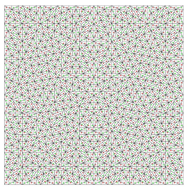
Figure 2: A patch of the pinwheel tiling. The control point in $\varLambda$ are coloured according to the two chiralities of the triangles.

The inflation rule $\sigma$ gives rise to the substitution matrix

$$M = \begin{pmatrix}e^{it0}+e^{it\pi}&2e^{it(2\varphi-\pi)}+e^{it(2\varphi+\frac{\pi}{2})}\\ 2e^{it\pi}+e^{it(-\frac{\pi}{2})}&e^{it(2\varphi)}+e^{it(2\varphi-\pi)}\end{pmatrix}$$ (7)

$$= \begin{pmatrix}1+y^{2}&2xy^{-1}+xy\\ 2y^{2}+1/y^{-1}&x+xy^{-2}\end{pmatrix}$$

where we set $x=e^{2i\varphi t}$ and $y=e^{i\pi t/2}$. This matrix was used in [12] to derive the circular symmetry of the autocorrelation. If we only wish to distinguish orientations modulo 90 degrees, we can choose $t=4$, so $y=1$, and the matrix simplifies to

$$M=\begin{pmatrix}2&3x\\ 3&2x\end{pmatrix}.$$ (8)

This matrix can be used to derive information about the subsets of control points that belong to the same direction, in the sense that they belong to the same power of $x$.

3 Hierarchies of subsets of different orientation

Let us consider what happens when we start from an initial patch containing one triangle of each chirality with horizontal orientation, and perform $n$ inflation steps. Denoting by $f^{\pm}_{n}(k)$ the number of triangles of each chirality at step $n$ with orientation factor $x^{k}$, where $0\leq k\leq n$, we find

$$\begin{pmatrix}\sum_{k=0}^{n}f^{+}_{n}(k)\,x^{k}\\ \sum_{k=0}^{n}f^{-}_{n}(k)\,x^{k}\end{pmatrix}\;=\;M^{n}\,\begin{pmatrix}1\\ 1\end{pmatrix}.$$ (9)

Multiplication by $M$ gives the following recursion for the coefficients

$$f^{+}_{n+1}(k) = 2\,f^{+}_{n}(k)+3\,f^{-}_{n}(k-1)\,,$$ (10a)

$$f^{-}_{n+1}(k) = 2\,f^{+}_{n}(k-1)+3\,f^{-}_{n}(k)\,,$$ (10b)

for $0\leq k\leq n+1$, where the appropriate initial conditions are $f^{\pm}_{0}(0)=1$ and $f^{\pm}_{n}(k)=0$ for all $k<0$ and $k>n$.

Clearly, these numbers satisfy the relation $f^{+}_{n}(k)=f^{-}_{n}(n-k)$ for all $0\leq k\leq n$, as can be seen from the relation

$$\begin{pmatrix}0&1\\ 1&0\end{pmatrix}\begin{pmatrix}2&3x\\ 3&2x\end{pmatrix}\begin{pmatrix}0&1\\ 1&0\end{pmatrix}\;=\;\begin{pmatrix}2x&3\\ 3x&2\end{pmatrix}\;=\;x\begin{pmatrix}2&3x^{-1}\\ 3&2x^{-1}\end{pmatrix}.$$ (11)

Hence the total number of triangles $f_{n}(k)=f^{+}_{n}(k)+f^{-}_{n}(k)$ obeys the symmetry $f_{n}(k)=f_{n}(n-k)$ for all $0\leq k\leq n$.

These observations have some interesting consequences. For instance, it can been shown that for even $n$

$$f_{n}^{+}(0)<f_{n}^{-}(0)<f_{n}^{+}(1)<f_{n}^{-}(1)<\ldots<f^{+}_{n}(\tfrac{n}{2}-1)<f^{-}_{n}(\tfrac{n}{2}-1)<f^{+}_{n}(\tfrac{n}{2})=f_{n}^{-}(\tfrac{n}{2})$$

and for odd $n$

$$f_{n}^{+}(0)<f_{n}^{-}(0)<f_{n}^{+}(1)<f_{n}^{-}(1)<\ldots<f^{+}_{n}(\tfrac{n-1}{2}-1)<f^{-}_{n}(\tfrac{n-1}{2}-1)<f^{+}_{n}(\tfrac{n-1}{2})=f_{n}^{-}(\tfrac{n+1}{2})\,.$$

It follows that $f_{n}(k)>f_{n}(k-1)$ for $1\leq k\leq[\frac{n}{2}]-1$, and the symmetry property $f_{n}(k)=f_{n}(n-k)$ then implies a corresponding inequality for large $k$.

4 Diffraction of pinwheel point sets

While it has been shown that the autocorrelation of the pinwheel point set is circularly symmetric [12], it is not known whether it is concentrated on sharp rings only, or whether there is also a continuous component. Direct numerical computations are of no help here, because any finite patch only contains a small number of independent directions, and is clearly not a good approximation of the limit structure. However, as shown in [1, 2], the knowledge that the diffraction is circularly symmetric can be exploited to derive an approximation of the diffraction based on a radial version of the Poisson summation formula; see [1] for details. This results in an expansion in terms of Bessel functions. As shown in [1, 2], this results in a radial distribution of the diffraction intensity that shows clear maxima for distances corresponding to those of a square lattice, so the radially discrete part resembles that of a powder diffraction of a square lattice. However, as the pinwheel structure contains a hierarchical sequence of scaled square lattices, the intensity distribution is not the same as for the square lattice, but deviates in a characteristic fashion. In addition, these numerical data provide an indication that there is also a continuous component.

Here, we consider the slightly generalised case of diffraction from weighted pinwheel sets. Circular symmetry also holds for the autocorrelation of a weighted pinwheel control point set, with weights depending on the two chiralities of the triangular tiles. This follows from [9, Thm. 6.1]: the triangles can be regarded as two prototiles, a left-handed and a right-handed one, and each individual prototile then shows circular symmetry, too.

Denoting the sets of pinwheel control points for the two chiralities by $\varLambda_{\pm}$, with $\varLambda_{+}\cup\varLambda_{-}=\varLambda$, we thus consider the weighted Dirac comb

$$\omega\;=\;\alpha_{+}\,\delta_{\varLambda_{+}}+\alpha_{-}\,\delta_{\varLambda_{-}}\;:=\;\sum_{x\in\varLambda_{+}}\alpha_{+}\,\delta_{x}+\sum_{x\in\varLambda_{-}}\alpha_{-}\,\delta_{x}\,,$$ (12)

where $\alpha_{\pm}$ are arbitrary, in general complex, weights. In this paper, we restrict ourselves to values $\alpha_{\pm}\in\{-1,0,1\}$, with the case $\alpha_{+}=\alpha_{-}=1$ corresponding to the pinwheel diffraction considered in [1, 2].

The approximations to the radial density distribution shown below are obtained by computing approximate autocorrelation coefficients $\eta(r)$ for distances $r$, obtained from finite approximants of the pinwheel tiling, up to a suitable maximum distance. The approximation to the autocorrelation then has the form

$$\gamma_{\omega}\;=\;\sum_{r\in\mathcal{D}}\eta(r)\,\mu_{r}\,,$$ (13)

where $\mu_{r}$ denotes the uniform measure on the unit circle, and

$$\mathcal{D}\subset\Bigl{\{}\sqrt{\frac{p^{2}+q^{2}}{5^{\ell}}}\;\Big{|}\;p,q,\ell\in\mathbb{N}\Bigr{\}}$$ (14)

denotes the distance set for the pinwheel tiling. Here, the assumption of circular symmetry enters — the approximate autocorrelation coefficients obtained from a finite patch are used to define a circularly symmetric autocorrelation measure. From Equation (13), the approximate radial distribution of the diffraction intensity $I(k)$ is obtained as the weighted sum of the Fourier transform of the uniform measure $\mu_{r}$. As the latter is given by $\widehat{\mu}_{r}(k)=J_{0}(2\pi|k|r)$, this results in finite sums of Bessel functions $J_{0}$ which show strong oscillations; compare [1, 2] for details. We note in passing that some values for frequencies of distances are known exactly, and they can in principle be computed from the inflation rule; see [13].

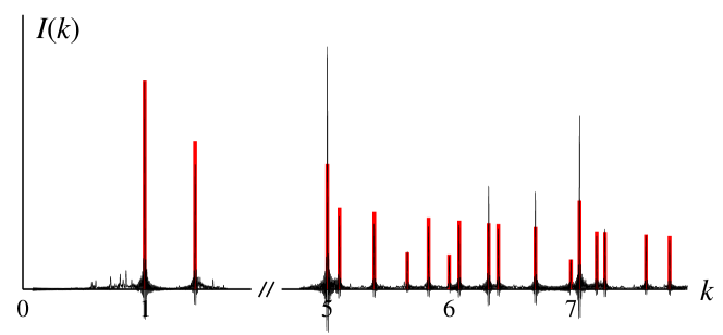
Figure 3: Part of the approximated radial intensity distribution for the pinwheel diffraction ($\alpha_{+}=\alpha_{-}=1$), compared with the exact diffraction for a square lattice powder (red bars).

4.1 Systematics of peak intensities

Figure 3 shows the numerical approximation for the diffraction of $\delta_{\varLambda}$, which is the pinwheel point sets with weights $\alpha_{+}=\alpha_{-}=1$. The corresponding result for a square lattice powder is also shown, with relative normalisation chosen to make the first peak match. Clearly, as observed in [1, 2], the main peaks in the intensity are well reproduced, but there are systematic deviations in the peak intensities. The latter can qualitatively be explained as arising from distances in $\mathcal{D}$ of Equation (14) with denominators $5^{\ell}$ with $\ell>0$.

To get a better picture of the peak intensities, we consider separately the integrated intensities on rings at values of $k$ according to the highest power of $5$ that divides $k^{2}$ (which will be $0$, $1$ or $2$ in the examples below). Figure 4 shows the result for the case where $k$ is not divisible by $5$. On the left, you can clearly distinguish three groups of data, indicated by different colours, and for each group of data the decay of intensities with increasing $k$ is well approximated by a function of the type $c/k$, where $c$ is a constant.

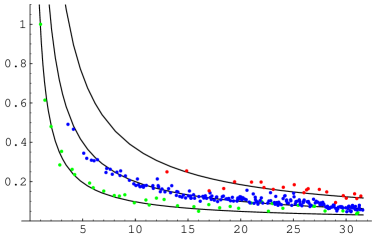
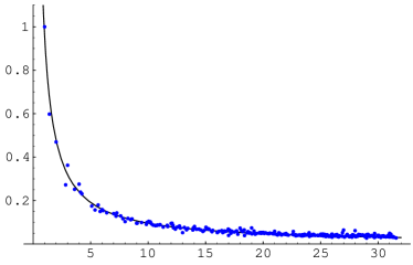
Figure 4: Intensity ratios $I(k)/I(1)$ of peaks for values of $k$ such that $k^{2}$ is not divisible by $5$, as a function of $k$. On the left, different colours refer to different number of prime factors equal to $1$ modulo $4$ (either $0$ (green), $1$ (blue) or $2$ (red)). Note that equal factors are counted here; for instance, the lowest $k$ in the second group is $k=\sqrt{13}$, and in the third group it is $k=\sqrt{169}=13$. On the right, these data have been collapsed as described in the text. Lines are least square fits to functions of the form $c/k$ with constant $c$.

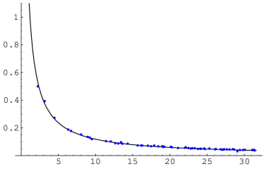
Figure 5: Same as right part of Figure 4, for values of $k$ such that $k^{2}$ is divisible by $5$ but not $5^{2}$ (left) and such that $k^{2}$ is divisible by $5^{2}$ but not by $5^{3}$ (right).

The three groups of data are distinguished by the number of prime factors of $k^{2}$ that are equal to $1$ modulo $4$. In fact, dividing the intensity ratios by $2^{s}$, where $s$ is the sum of powers of all prime factors of this type, collapses the data set onto a single curve, as shown in the right part of Figure 4. This observation is in line with the similarity to the square lattice powder diffraction seen in [1, 2].

The corresponding collapsed data for peaks at values of $k$ which are multiples of $5$ and $5^{2}$ are shown on the left and right of Figure 5, respectively. Again, the observed decay of the intensities is inversely proportional to $k$. This indicates that our qualitative understanding of the peak intensities is correct, though it is not clear whether this also holds quantitatively for the diffraction of an infinite pinwheel tiling point set.

4.2 Diffraction of weighted pinwheel point sets

In order to get a better indication of the possible continuous contribution of the pinwheel diffraction, it is advantageous to consider weighted pinwheel point sets. As discussed above, the resulting autocorrelation is still circularly symmetric, and hence the same approach as outlined above can be applied to obtain approximations of the radial intensity distribution. Figure 6 shows the result for the case $\omega=\delta_{\varLambda_{+}}$ ($\alpha_{+}=1$ and $\alpha_{-}=0$), where only the half of the pinwheel point set is considered. The three spectra correspond to an increasing number of terms in the approximation, and increasing accuracy of the estimated correlation coefficients from larger patches of the pinwheel tiling constructed by successive inflation. The result very closely resembles that for the complete pinwheel point set, and may well be identical apart from the overall intensity normalisation due to the different density of scatterers.

Figure 6: Three approximations of the radial intensity distribution of the diffraction of the Dirac comb $\delta_{\varLambda_{+}}$.

More interesting is the case of $\alpha_{+}=1$ and $\alpha_{-}=-1$. Since this is a balanced case, the average scattering strength is zero, and there is no peak at $k=0$. Therefore, a continuous background may be easier to spot in this case. Figure 7 shows three increasingly accurate approximations of the radial diffraction intensity for this case.

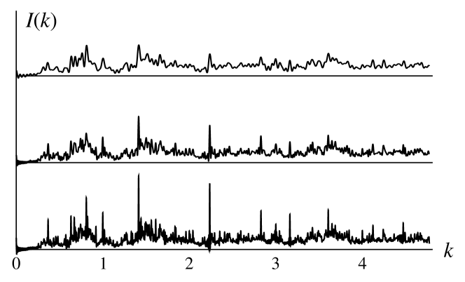
Figure 7: Three approximations of the radial intensity distribution of the diffraction of the Dirac comb $\omega$ for the balanced case with $\alpha_{+}=1$ and $\alpha_{-}=-1$.

There is not only an indication of the presence of a continuous background, similar to what was found in [2], but also a number of new features appear to develop (in particular for small values of $k$), which may correspond to additional peaks for the infinite system. However, the approximation may not yet be good enough to draw firm conclusions.

5 Summary

The diffraction of substitution tilings with continuous rotational symmetry still remains to be completely understood. In this paper, we presented some observations on combinatorial properties of the pinwheel tiling and on its diffraction measure, using the approximation introduced in [1, 2]. From the numerical data, we corroborate the conclusions of [1, 2] on the similarities between the pinwheel diffraction and a square lattice powder. Considering the balanced case of zero average scattering strength provides an indication that there might not only be a continuous contribution as conjectured in [2], but that there might also be additional sharp rings with finite intensity. This observation warrants further investigation. It would also be interesting to compare this result with the diffraction of other tilings, such as the generalised pinwheel tilings introduced by Sadun [18] or the tipi tilings in [9].

References

- [1] Baake M, Frettlöh D and Grimm U 2007 A radial analogue of Poisson’s summation formula with applications to powder diffraction and pinwheel patterns J. Geom. Phys. 57 1331–1343
- [2] Baake M, Frettlöh D and Grimm U 2007 Pinwheel patterns and powder diffraction Philos. Mag. 87 2831–2838
- [3] Baake M and Grimm U 2009 Kinematic diffraction is insufficient to distinguish order from disorder Phys. Rev. B 79 020203(R) and 80 029903(E)
- [4] Baake M and Grimm U 2010 Surprises in aperiodic diffraction J. Physics: Conf. Ser. 226 012023
- [5] Baake M and Grimm U 2011 Mathematical diffraction theory of deterministic and stochastic structures: an informal summary RIMS proceedings (in press)
- [6] Baake M and Grimm U Kinematic diffraction from a mathematical viewpoint (in preparation)
- [7] Baake M and Grimm U Theory of Aperiodic Order: A Mathematical Invitation (Cambridge: CUP, in preparation)
- [8] Baake M, Schlottmann M and Jarvis PD 1991 Quasiperiodic tilings with tenfold symmetry and equivalence with respect to local derivability J. Phys. A: Math. Gen. 24 4637–4654
- [9] Frettlöh D 2008 Substitution tilings with statistical circular symmetry Eur. J. Combin. 29 1881–1893
- [10] Ishimasa T, Nissen H-U and Fukano Y 1985 New ordered state between crystalline and amorphous in Ni-Cr particles Phys. Rev. Lett. 55 511–513
- [11] Lenz D 2008 Aperiodic order and pure point diffraction Philos. Mag. 88 2059–2071
- [12] Moody R V, Postnikoff D and Strungaru N 2006 Circular symmetry of pinwheel diffraction Ann. Henri Poincaré 7 711–730
- [13] Moustafa H 2009 PV cohomology of pinwheel tilings, their integer group of coinvariants and gap-labelling Preprint arXiv:0906.2107
- [14] Radin C 1994 The pinwheel tilings of the plane Ann. Math. 139 661–702
- [15] Radin C 1995 Space tilings and substitutions Geometriae Dedicata 55 257–264
- [16] Radin C 1997 Aperiodic tilings, ergodic theory and rotations The Mathematics of Long-Range Aperiodic Order (NATO ASI C 489) ed RV Moody (Dordrecht: Kluwer) pp 499–519
- [17] Radin C 1999 Miles of Tiles (Providence: AMS)
- [18] Sadun L 1998 Some generalizations of the pinwheel tiling Discrete Comput. Geom. 20 79–100
- [19] Shechtman D, Blech I, Gratias D and Cahn J W 1984 Metallic phase with long-range orientational order and no translational symmetry Phys. Rev. Lett. 53 1951–1953