Nucleation and growth for the Ising model in $d$ dimensions at very low temperatures

Abstract

This work extends to dimension $d\geq 3$ the main result of Dehghanpour and Schonmann. We consider the stochastic Ising model on ${\mathbb{Z}}^{d}$ evolving with the Metropolis dynamics under a fixed small positive magnetic field $h$ starting from the minus phase. When the inverse temperature $\beta$ goes to $\infty$, the relaxation time of the system, defined as the time when the plus phase has invaded the origin, behaves like $\exp({{\beta}{\kappa}_{d}})$. The value $\kappa_{d}$ is equal to

$${\kappa}_{d}=\frac{1}{d+1}({\Gamma}_{1}+\cdots+{\Gamma}_{d}),$$

where ${\Gamma}_{i}$ is the energy of the $i$-dimensional critical droplet of the Ising model at zero temperature and magnetic field $h$.

and

[level=2]

1 Introduction

We consider the kinetic Ising model in ${\mathbb{Z}}^{d}$ under a small positive magnetic field in the limit of vanishing temperature, and we study the relaxation of the system starting from the metastable state where all the spins are set to minus. An introduction of the metastability problem is presented in Section 1.1. In Section 1.2, we explain the three major problems we had to solve to extend the two-dimensional results to dimension $d$. The main results are stated in Section 1.3. The strategy of the proof is explained in Section 1.4.

1.1 Background

This work extends to dimension $d\geq 3$ the main result of Dehghanpour and Schonmann DS1 . We consider the stochastic Ising model on ${\mathbb{Z}}^{d}$ evolving with the Metropolis dynamics under a fixed small positive magnetic field $h$. We start the system in the minus phase. Let $\tau_{d}$ be the typical relaxation time of the system, defined here as the time where the plus phase has invaded the origin. We will study the asymptotic behavior of $\tau_{d}$ when we scale the temperature to $0$. The corresponding problem in finite volume (i.e., in a box $\Lambda$ whose size is fixed) has been previously studied in arbitrary dimension by Neves N2 , N1 . In this situation, Neves proved that the relaxation time behaves as $\exp(\beta\Gamma_{d})$ where $\beta=1/T$ is the inverse temperature, and $\Gamma_{d}$ is the energy barrier the system has to overcome to go from the metastable state $\mathbf{-1}$ to the stable state $\mathbf{+1}$. An explicit formula is available for $\Gamma_{d}$; however the formula is quite complicated. The energy barrier $\Gamma_{d}$ is the solution of a minimax problem, and it is reached for configurations which are optimal saddles between $\mathbf{-1}$ and $\mathbf{+1}$ in the energy landscape of the Ising model. These results have been refined in dimension $3$ in BAC . In dimension $3$, the optimal saddles are identified. They are configurations called critical droplets which contain exactly one connected component of pluses of cardinality $m_{3}$, and their shape is an appropriate union of a specific quasicube (whose sides depend on $h$) and a two-dimensional critical droplet. In dimension $d\geq 4$, the results of Neves yield that the configurations consisting of the appropriate union of a $d$-dimensional quasicube and a $(d-1)$-dimensional critical droplet are optimal saddles, but it is currently not proved that they are the only ones. However, it is reasonable to expect that the cases of equality in the discrete isoperimetric inequality on the lattice can be analyzed in dimension $d\geq 4$ in the same way they were studied in dimension $d=3$ AC , so that the three-dimensional results could be extended to higher dimensions.

In infinite volume, instead of nucleating locally in a finite box near the origin, a critical droplet of pluses might be created far from the origin, and this droplet can grow, become supercritical and invade the origin. It turns out that this is the most efficient mechanism to relax to equilibrium. This was shown by Dehghanpour and Schonmann in the two-dimensional case DS1 and it required several new ideas and insights compared to the finite volume analysis. Indeed, one has to understand the typical birth place of the first critical droplets which are likely to invade the origin, as well as their growth mechanism. The heuristics given in DS1 apply in $d$ dimensions as well. Suppose that nucleation in a finite box is exponentially distributed with rate $\exp({-{\beta}{\Gamma}_{d}})$, independently from other boxes, and that the speed of growth of a large supercritical droplet is $v_{d}$. The droplets which can reach the origin at time $t$ are the droplets which are born inside the space–time cone whose basis is a $d$-dimensional square with side length $v_{d}t$ and whose height is $t$. The critical space–time cone is such that its volume times the nucleation rate is of order one. Let ${\tau}_{d}$ be the typical relaxation time in dimension $d$, that is, the time when the stable plus phase invades the origin. From the previous heuristics, we conclude that ${\tau}_{d}$ satisfies

$$\tfrac{1}{3}{\tau}_{d}(v_{d}{\tau}_{d})^{d}\exp({-{\beta}{\Gamma}_{d}})=1.$$

Solving this identity and neglecting the factor ${1}/{3}$, we get

$${\tau}_{d}=\exp\biggl{(}\frac{1}{d+1}(\beta{\Gamma}_{d}-d\ln v_{d})\biggr{)}.$$

Since the large supercritical droplets are approximately parallelepipeds, the dynamics on one face behaves like a $(d-1)$-dimensional stochastic Ising model, and the time needed to fill a face with pluses is of order $\tau_{d-1}$. Thus $v_{d}$ should behave like the inverse of $\tau_{d-1}$, and the previous formula becomes

$$\ln{\tau}_{d}=\frac{1}{d+1}(\beta{\Gamma}_{d}+d\ln{\tau}_{d-1}).$$

In this computation, we take only into account the terms on the exponential scale, of order $\exp(\beta\mbox{ constant})$. Setting ${\tau}_{d}=\exp({{\beta}{\kappa}_{d}})$, the constant ${\kappa}_{d}$ satisfies

$${\kappa}_{d}=\frac{1}{d+1}({\Gamma}_{d}+d{\kappa}_{d-1}).$$

Solving the recursion, and using that ${\kappa}_{0}=0$, we get that

$${\kappa}_{d}=\frac{1}{d+1}({\Gamma}_{1}+\cdots+{\Gamma}_{d}).$$

1.2 Three major problems

Although these heuristics are rather convincing, it is a real challenge to prove rigorously that the asymptotics of the relaxation time are indeed of order $\exp({{\beta}{\kappa}_{d}})$. Our strategy is to implement inductively the scheme of Dehghanpour and Schonmann. To do so, we had to overcome three major problems.

Speed of growth. A first major difficulty is to control the speed of growth $v_{d}$ of large supercritical droplets. The upper bound on the speed of growth in DS2 was based on a very detailed analysis of the growth of an infinite interface. Using a combinatorial argument based on chronological paths, first introduced by Kesten and Schonmann in the context of a simplified growth model KS , Dehghanpour and Schonmann were able to prove that $v_{2}$ is of order $\exp(-\beta\Gamma_{1}/2)$. Despite considerable efforts, we never managed to extend this technique of analysis to higher dimension. Here we consider only interfaces with a size that is exponential in ${\beta}$. In order to control the growth of these interfaces, we use inductively coupling techniques introduced to analyze the finite-size scaling in the bootstrap percolation model CeCi , CM . We apply successively these techniques in two distinct ways, the first sequential and the second parallel. This strategy has been elaborated first in a simplified growth model CM2 , yet its application in the context of the Ising model is more troublesome. Contrary to the case of the growth model, we did not manage to compare the dynamics in a strip with a genuine $(d-1)$-dimensional dynamics, and we perform the induction on the boundary conditions rather than on the dimension. An additional source of trouble is to control the configurations in the metastable regions. We introduce an adequate hypothesis describing their law, which is preserved until the arrival of supercritical droplets, in order to tackle this problem. A key result to control the speed of growth is Theorem 6.4.

Energy landscape. A second major difficulty is that it is very hard to analyze the energy landscape of the Ising model in high dimension, and the results we are able to obtain are very weak compared to the corresponding results in finite volume and in dimensions two and three; see NS1 , NS2 , BAC . For instance we are not able to determine whether a given cluster of pluses tends to shrink or to grow. Moreover, we do not know some of the fine details of the energy landscape such as the depth of the small cycles that could trap the process and increase the relaxation time. In other words, we do not know how to compute the inner resistance of the metastable cycle in $d$ dimensions, that is, the energy barrier that a subcritical configuration has to overcome in order to reach either the plus configuration or the minus configuration in a finite box. This fact affects both strategies for the upper as well as for the lower estimate of the relaxation time, since in order to approximate the distribution of the nucleation time as an exponential law with rate $\exp(-{\beta}{\Gamma}_{d})$, one has to rule out the possibility that the process is trapped in a deep well. We are able to get the required bounds by using the attractivity and the reversibility of the dynamics; see Lemma 6.1 and Proposition 7.4.

Space–time clusters. The third major difficulty to extend the analysis of Dehghanpour and Schonmann is to control adequately the space–time clusters. For instance, we cannot proceed as in DS1 to rule out the possibility that a subcritical cluster crosses a long distance. This question turns out to be much more involved in higher dimension. It is tackled in Theorem 5.7, which is a key of the whole analysis. To control the diameters of the space–time clusters, we use ideas of recurrence and a decomposition of the space into sets called “cycle compounds.” A cycle compound is a connected set of states $\overline{\cal A}$ such that the communication energy between two points of $\overline{\cal A}$ is less than or equal to the communication energy between $\overline{\cal A}$ and its complement. A cycle is a cycle compound, yet an appropriate union of cycles might form a cycle compound without being a cycle.

1.3 Main results

We now briefly describe the model, and we state next our main result. We study the $d$-dimensional nearest-neighbor stochastic Ising model at inverse temperature $\beta$ with a fixed small positive magnetic field $h$, that is, the continuous-time Markov process $(\sigma_{t})_{t\geq 0}$ with state space $\{-1,+1\}^{{\mathbb{Z}}^{d}}$ defined as follows. In the configuration $\sigma$, the spin at the site $x\in{\mathbb{Z}}^{d}$ flips at rate

$$c\bigl{(}\sigma,\sigma^{x}\bigr{)}=\exp\bigl{(}-\beta\bigl{(}\Delta_{x}H(\sigma)\bigr{)}^{+}\bigr{)},$$

where $(a)^{+}=\max(a,0)$ and

$$\Delta_{x}H(\sigma)=\sigma(x)\biggl{(}\mathop{\sum_{y\in{\mathbb{Z}}^{d}}}_{|x-y|=1}\sigma(y)+h\biggr{)}.$$

In other words, the infinitesimal generator of the process $(\sigma_{t})_{t\geq 0}$ acts on a local observable $f$ as

$$(Lf)(\sigma)=\sum_{x}c\bigl{(}\sigma,\sigma^{x}\bigr{)}\bigl{(}f\bigl{(}\sigma^{x}\bigr{)}-f(\sigma)\bigr{)},$$

where $\sigma^{x}$ is the configuration $\sigma$ in which the spin at site $x$ has been turned upside down. Formally, we have

$$\Delta_{x}H(\sigma)=H\bigl{(}\sigma^{x}\bigr{)}-H(\sigma),$$

where $H$ is the formal Hamiltonian given by

$$H(\sigma)=-\frac{1}{2}\mathop{\sum_{\{x,y\}\subset{\mathbb{Z}}^{d}}}_{|x-y|=1}\sigma(x)\sigma(y)-\frac{h}{2}\sum_{x\in{\mathbb{Z}}^{d}}\sigma(x).$$

More details on the construction of this process are given in Sections 3.1 and 3.2. We denote by $({\sigma}_{t}^{\mathbf{-1}})_{t\geq 0}$ the process starting from $\mathbf{-1}$, the configuration in which all the spins are equal to $-1$. A local observable is a real valued function $f$ defined on the configuration space which depends only on a finite set of spin variables.

Theorem 1.1

Let $f$ be a local observable. If the magnetic field $h$ is positive and sufficiently small, then there exists a value ${\kappa}_{d}$ such that, letting ${\tau_{\beta}}=\exp(\beta{\kappa})$, we have

$$\lim_{\beta\to\infty}E\bigl{(}f\bigl{(}{\sigma}_{{{\tau_{\beta}}}}^{\mathbf{-1}}\bigr{)}\bigr{)} = f(\mathbf{-1})\qquad\mbox{if }{\kappa}<{\kappa}_{d},$$

$$\lim_{\beta\to\infty}E\bigl{(}f\bigl{(}{\sigma}_{{\tau_{\beta}}}^{\mathbf{-1}}\bigr{)}\bigr{)} = f(\mathbf{+1})\qquad\mbox{if }{\kappa}>{\kappa}_{d}.$$

The value ${\kappa}_{d}$ depends only on the dimension $d$ and the magnetic field $h$; in fact, if we denote by ${\Gamma}_{i}$ the energy of the $i$-dimensional critical droplet of the Ising model at zero temperature and magnetic field $h$, then

$${\kappa}_{d}=\frac{1}{d+1}({\Gamma}_{1}+\cdots+{\Gamma}_{d}).$$

Besides the aforementioned technical difficulties, our proof is basically an inductive implementation of the scheme of DS1 , combined with the strategy of CM . The first step of the proof consists in reducing the problem to a process defined in a finite exponential volume. Let $\kappa>0$, and let $\tau_{\beta}=\exp(\beta{\kappa})$. Let $L>\kappa$, and let ${\Lambda}_{\beta}={\Lambda}(\exp(\beta L))$ be a cubic box of side length $\exp(\beta L)$. We have that

$$\lim_{\beta\to{\infty}}P\bigl{(}f\bigl{(}{\sigma}_{\tau_{\beta}}^{\mathbf{-1}}\bigr{)}=f\bigl{(}{\sigma}_{{\Lambda}_{\beta},\tau_{\beta}}^{-,\mathbf{-1}}\bigr{)}\bigr{)}=1,$$

where $({\sigma}_{{\Lambda}_{\beta},t}^{-,\mathbf{-1}})_{t\geq 0}$ is the process in the box ${\Lambda}_{\beta}$ with minus boundary conditions starting from $\mathbf{-1}$. This follows from a standard large deviation estimate based on the fact that the maximum rate in the model is $1$; see Lemmas 1, 2 of Sch for the complete proof. We state next the finite volume results that we will prove.

Theorem 1.2

Let $L>0$, and let ${\Lambda}_{\beta}={\Lambda}(\exp(\beta L))$ be a cubic box of side length $\exp(\beta L)$. Let $\kappa>0$, and let $\tau_{\beta}=\exp(\beta{\kappa})$. There exists $h_{0}>0$ such that, for any $h\in\ ]0,h_{0}[$, the following holds:

$\bullet$ If $\kappa<\max(\Gamma_{d}-dL,\kappa_{d})$, then

$$\lim_{\beta\to\infty}P\bigl{(}{\sigma}_{{\Lambda}_{\beta},\tau_{\beta}}^{-,\mathbf{-1}}(0)=1\bigr{)}=0.$$

$\bullet$ If $\kappa>\max(\Gamma_{d}-dL,\kappa_{d})$, then

$$\lim_{\beta\to\infty}P\bigl{(}{\sigma}_{{\Lambda}_{\beta},\tau_{\beta}}^{-,\mathbf{-1}}(0)=-1\bigr{)}=0.$$

Recall that $\Gamma_{d}$ and $\kappa_{d}$ depend on the magnetic field $h$. Explicit formulas are available for $\Gamma_{d}$ and $\kappa_{d}$; however, they are quite complicated. An important point is that $\Gamma_{d}$ and $\kappa_{d}$ are continuous functions of the magnetic field $h$ (this is proved in Lemma 4.1), and this will allow us to reduce the study to irrational values of $h$. An explicit bound on $h_{0}$ can also be computed. In dimension $d$, the proof works if $h_{0}\leq 1$ and Lemma 6.8 holds. Let us denote by $m_{d}$ the volume of the critical droplet in dimension $d$. Lemma 6.8 holds as soon as

$$\forall n\leq d\qquad(\Gamma_{n-1})^{{n}}\leq(m_{n-1})^{n-1}.$$

We next shift our attention to finite volumes, and we try to perform simple computations to understand why the critical constant appearing in Theorem 1.2 is equal to $\max(\Gamma_{d}-dL,\kappa_{d})$. We have two possible scenarios for the relaxation to equilibrium in a finite cube. If the cube is small, then the system relaxes via the formation of a single critical droplet that grows until covering the entire volume. If the cube is large, then we have a more efficient mechanism, creating many critical droplets that grow and eventually coalesce. The critical side length of the cubes separating these two mechanisms scales exponentially with ${\beta}$ as $\exp({\beta}L_{d})$, where

$$L_{d}=\frac{\Gamma_{d}-\kappa_{d}}{d}.$$

This value is the result of the computations, and we do not have a simple heuristic explanation for it. There are three main factors controlling the relaxation time, which correspond to the heuristics explained previously:

Nucleation. Within a box of side length $\exp(\beta K)$, the typical time when the first critical droplet appears is of order $\exp(\beta(\Gamma_{d}-dK))$.

Initial growth. The typical time to grow from a critical droplet (which has a diameter of order $2d/h$) into a supercritical droplet [which has a diameter of order $\exp({\beta}L_{d})$] traveling at the asymptotic speed $\exp(-\beta\kappa_{d-1})$ is $\exp(\beta\Gamma_{d-1})$.

Asymptotic growth. In a time $\exp(\beta(K+\kappa_{d-1}))$, a supercritical droplet having a diameter larger than $\exp({\beta}L_{d})$ and traveling at the asymptotic speed $\exp(-\beta\kappa_{d-1})$ covers a distance $\exp(\beta K)$ in each axis direction and its diameter increases by $2\exp(\beta K)$.

The statement concerning the nucleation time contains no mystery. Let us try to explain the statements on the growth of the droplets. Once a critical droplet is born, it starts to grow at speed $\exp(-\beta\Gamma_{d-1})$. As the droplet grows, the speed of growth increases because the number of choices for the creation of a new $(d-1)$-dimensional critical droplet attached to the face of the droplet is of order the surface of the droplet. Thus the speed of growth of a droplet of size $\exp(\beta K)$ is

$$\exp\bigl{(}\beta\bigl{(}K(d-1)-\Gamma_{d-1}\bigr{)}\bigr{)}.$$

When $K$ reaches the value $L_{d-1}$, the speed of growth is limited by the inverse of the time needed for the $(d-1)$-dimensional critical droplet to cover an entire face of the droplet. This time corresponds to the $(d-1)$-dimensional relaxation time in infinite volume, and the droplet reaches its asymptotic speed, of order $\exp(-\beta\kappa_{d-1})$. The time needed to grow a critical droplet into a supercritical droplet traveling at the asymptotic speed is

$$\sum_{1\leq i\leq\exp(\beta L_{d-1})}\exp\biggl{(}\beta\biggl{(}\Gamma_{d-1}-\frac{d-1}{\beta}\ln i\biggr{)}\biggr{)}$$

and, for $d\geq 2$, this is still of order $\exp(\beta\Gamma_{d-1})$. With the help of the above facts, we can estimate the relaxation time in a box of side length $\exp(\beta L)$. Suppose that the origin is covered by a large supercritical droplet at time $\exp(\beta\kappa)$. If this droplet is born at distance $\frac{1}{2}\exp(\beta K)$, then nucleation has occurred inside the box ${\Lambda}(\exp(\beta K))$, and the initial critical droplet has grown into a droplet of diameter $\frac{1}{2}\exp(\beta K)$ in order to reach the origin. This scenario needs a time

$$\pmatrix{\mbox{time for nucleation}\cr\mbox{in the box ${\Lambda}\bigl{(}\exp(\beta K)\bigr{)}$}}+\pmatrix{\mbox{time to cover}\cr\mbox{the box ${\Lambda}\bigl{(}\exp(\beta K)\bigr{)}$}}$$

$$\qquad\sim\exp\bigl{(}\beta(\Gamma_{d}-dK)\bigr{)}+\exp(\beta\Gamma_{d-1})+\exp\bigl{(}\beta(K+\kappa_{d-1})\bigr{)},$$

which is of order

$$\exp\bigl{(}\beta\max(\Gamma_{d}-dK,\Gamma_{d-1},K+\kappa_{d-1})\bigr{)}.$$

To find the most efficient scenario, we optimize over $K<L$, and we conclude that the relaxation time in the box ${\Lambda}(\exp({\beta}L))$ is of order

$$\exp\Bigl{(}\beta\inf_{K\leq L}\max(\Gamma_{d}-dK,\Gamma_{d-1},K+\kappa_{d-1})\Bigr{)}.$$

It turns out that, for $h$ small, the above quantity is equal to

$$\exp\bigl{(}\beta\max(\Gamma_{d}-dL,\kappa_{d})\bigr{)}.$$

In particular, the time needed to grow a critical droplet into a supercritical droplet is not a limiting factor for the relaxation whenever $h$ is small.

1.4 Strategy of the proof

The upper bound on the relaxation time, that is, the second case where $\kappa>\max(\Gamma_{d}-dL,\kappa_{d})$, is done in Section 7. The ingredients involved in the upper bound are known since the works of Neves, Dehghanpour and Schonmann, and this part is considerably easier than the lower bound. The hardest part of Theorem 1.2 is the lower bound on the relaxation time, that is, the first case where $\kappa<\max(\Gamma_{d}-dL,\kappa_{d})$. The lower bound is done in Sections 5 and 6. Let us explain the strategy of the proof of the lower bound, without stating precisely the definitions and the technical results.

Let $L>0$ and let ${\Lambda}_{\beta}={\Lambda}(\exp(\beta L))$ be a cubic box of side length $\exp(\beta L)$. Let $\kappa>0$ and let $\tau_{\beta}=\exp(\beta{\kappa})$. We want to prove that it is unlikely that the spin at the origin is equal to $+1$ at time ${\tau_{\beta}}$ for the process $({\sigma}_{{\Lambda}_{\beta},t}^{-,\mathbf{-1}})_{t\geq 0}$. Throughout the proof, we use in a crucial way the notion of space–time cluster. A space–time cluster of the trajectory $(\sigma_{{\Lambda},t},{0\leq t\leq{\tau_{\beta}}})$ is a maximal connected component of space–time points for the following relation: two space–time points $(x,t)$ and $(y,s)$ are connected if $\sigma_{{\Lambda},t}(x)=\sigma_{{\Lambda},s}(y)=+1$ and either ($s=t$ and $|x-y|\leq 1$) or [$x=y$ and $\sigma_{{\Lambda},u}(x)=+1$ for $s\leq u\leq t$]. With the space–time clusters, we record the influence of the plus spins throughout the evolution. We can then compare the status of a spin in dynamics associated to different boundary conditions with the help of the graphical construction (described in Section 3.2). The diameter $\operatorname{diam}_{\infty}{\cal C}$ of a space–time cluster ${\cal C}$ is the diameter of its spatial projection. We argue as follows. If ${\sigma}_{{\Lambda}_{\beta},{\tau_{\beta}}}^{-,\mathbf{-1}}(0)=+1$, then the space–time point $(0,{\tau_{\beta}})$ belongs to a nonvoid space–time cluster, which we denote by ${\cal C}^{*}$. We discuss then according to the diameter of ${\cal C}^{*}$.

$\bullet$ If $\operatorname{diam}_{\infty}{\cal C}^{*}<\ln\ln\beta$, then ${\cal C}^{*}$ is also a space–time cluster of the process $({\sigma}_{{\Lambda}(\ln\beta),t}^{-,\mathbf{-1}},0\leq t\leq{\tau_{\beta}})$, and the spin at the origin is also equal to $+1$ in this process at time ${\tau_{\beta}}$. The finite volume estimates obtained for fixed boxes can be readily extended to boxes of side length $\ln\beta$, and we obtain that the probability of the above event is exponentially small if $\kappa<\Gamma_{d}$, because the entropic contribution to the free energy is negligible with respect to the energy.

$\bullet$ If $\operatorname{diam}_{\infty}{\cal C}^{*}>\exp(\beta L_{d})$ (this case can occur only when $L>L_{d}$), then we use the main technical estimate of the paper, Theorem 6.4, which states roughly the following: for $\kappa<\kappa_{d}$, the probability that, in the trajectory $({\sigma}_{{\Lambda}_{\beta},t}^{-,\mathbf{-1}},0\leq t\leq{\tau_{\beta}})$, there exists a space–time cluster of diameter larger than $\exp({{\beta}L_{d}})$ is a super exponentially small function of $\beta$ (denoted by ses in the following), and it can be neglected.

$\bullet$ If $\ln\ln\beta\leq\operatorname{diam}_{\infty}{\cal C}^{*}\leq\exp(\beta L_{d})$, then ${\cal C}^{*}$ is also a space–time cluster of the process restricted to the box ${\Lambda}(3\exp(\beta L_{d}))\cap{\Lambda}_{\beta}$. A space–time cluster is said to be large if its diameter is larger than or equal to $\ln\ln\beta$. A box is said to be small if its sides have a length larger than $\ln\ln\beta$ and smaller than $d\ln\beta$. The diameters of the space–time clusters increase with time when they coalesce because of a spin flip. This implies that if a large space–time cluster is created in the box ${\Lambda}_{\beta}$, then it has to be created first locally in a small box. The number of small boxes included in ${\Lambda}_{\beta}$ is of order

$$\bigl{|}{\Lambda}\bigl{(}3\exp(\beta L_{d})\bigr{)}\cap{\Lambda}_{\beta}\bigr{|}=\exp\bigl{(}\beta d\min(L_{d},L)\bigr{)}.$$

For the dynamics restricted to a small box, we have

$$P\pmatrix{\mbox{a large $\operatorname{\mbox{{stc}}}$ is}\cr\mbox{created before ${\tau_{\beta}}$}} \leq P\pmatrix{\mbox{a large $\operatorname{\mbox{{stc}}}$ is created}\cr\mbox{before nucleation}}$$

$${}+P\pmatrix{\mbox{nucleation occurs}\cr\mbox{before ${\tau_{\beta}}$}}.$$

The main result of Section 5.5, Theorem 5.7, yields that the first term of the right-hand side is ses. The finite volume estimates in fixed boxes obtained in the previous studies of metastability can be readily extended to small boxes. By Lemma 6.1, we have that, up to corrective factors,

$$P\pmatrix{\mbox{nucleation occurs}\cr\mbox{before ${\tau_{\beta}}$}}\leq\tau_{\beta}\exp(-{\beta}{\Gamma}_{d}).$$

Finally, we have

$$P\bigl{(}\operatorname{diam}_{\infty}{\cal C}^{*}\geq\ln\ln\beta\bigr{)} \leq \exp\bigl{(}\beta d\min(L_{d},L)\bigr{)}\bigl{(}\tau_{\beta}\exp(-{\beta}{\Gamma}_{d})+\mbox{{ses}}\bigr{)}$$

$$\leq \exp\bigl{(}\beta\bigl{(}d\min(L_{d},L)+\kappa-{\Gamma}_{d}\bigr{)}\bigr{)}+\mbox{{ses}}$$

$$= \exp\bigl{(}\beta\bigl{(}\kappa-\max({\Gamma}_{d}-dL_{d},{\Gamma}_{d}-dL)\bigr{)}\bigr{)}+\mbox{{ses}},$$

and the desired result follows easily.

From this quick sketch of proof, we see that the most difficult intermediate results are Theorems 5.7 and 6.4. The remainder of the paper is mainly devoted to the proof of these results. In Section 2, we consider a general Metropolis dynamics on a finite state space, we recall the formulas for the law of exit in continuous time and we introduce the notions of cycle and cycle compound in this context. Section 3 is devoted to the study of some specific features of the cycle compounds of the Ising model. In Section 4, we state several discrete isoperimetric results from N2 , N1 , AC . Apart from the notion of cycle compound, the definitions and the results presented in Sections 2, 3 and 4 come from the previous literature on metastability, with some rewriting and adaptation to fit the continuous-time framework and our specific $n\pm$ boundary conditions. The main technical contributions of this work are presented in Sections 5 and 6. In Section 5, we prove the key estimate on the diameters of the space–time clusters (Theorem 5.7). Section 6 is devoted to the proof of Theorem 6.4. The proof of the lower bound on the relaxation time is completed in Section 6.5. The final section, Section 7, contains the proof of the upper bound on the relaxation time.

2 The Metropolis dynamics

A very efficient tool for describing the metastable behavior of a process in the low temperature regime is a hierarchical decomposition of the state space known as the cycle decomposition. In the context of a Markov chain with finite state space evolving under a Metropolis dynamics, the cycles can be defined geometrically with the help of the energy landscape. Our context of infinite volume is much more complicated, but since the system is attractive, we will end up with some local problems that we handle with the finite volume techniques. We start by reviewing these techniques. Here we recall some basic facts about the cycle decomposition. For a complete review we refer to S4 , OS3 , OS2 , CaCe , OS1 , OV . Since we are working here with a continuous-time process defined with the help of transition rates, as opposed to a discrete-time Markov chain defined with transition probabilities, we feel that it is worthwhile to present the exact formulas giving the law of exit of an arbitrary subset in this slightly different framework. This is the purpose of Section 2.1. In Section 2.2, we define the Metropolis dynamics, and we show how to apply the formulas of Section 2.1 to this specific dynamics. In Section 2.3, we recall the definitions of a cycle, the communication energy, the height of a set, its bottom, its depth and its boundary. We introduce also an additional concept, called cycle compound, which turns out to be useful when analyzing the energy landscape of the Ising model. Apart from the notion of cycle compounds, the definitions and the results presented in this section come from the previous literature on metastability and simulated annealing, they are simply adapted to the continuous-time framework.

2.1 Law of exit

We will not derive in detail all the results used in this paper concerning the behavior of a Markov process with exponentially vanishing transition rates because the proofs are essentially the same as in the discrete-time setting. These proofs can be found in the book of Freidlin and Wentzell (FW , Chapter $6$, Section $3$), or in the lecture notes of Catoni (Catoni , Section $3$). However, for the sake of clarity, we present the two basic formulas in continuous time giving the law of the exit from an arbitrary set. Let ${\cal X}$ be a finite state space. Let $c\dvtx{\cal X}\times{\cal X}\to{\mathbb{R}}$ be a matrix of transition rates on ${\cal X}$, that is,

$$\displaystyle\forall x,y\in{\cal X},\qquad x\neq y,\qquad c(x,y)\geq 0,$$

$$\displaystyle\forall x\in{\cal X}\qquad\sum_{y\in{\cal X}}c(x,y)=0.$$

We consider the continuous-time homogeneous Markov process $(X_{t})_{t\geq 0}$ on ${\cal X}$ whose infinitesimal generator is

$$\forall f\dvtx{\cal X}\to{\mathbb{R}}\qquad(Lf)(x)=\sum_{y\in{\cal X}}c(x,y)\bigl{(}f(y)-f(x)\bigr{)}.$$

For $C$ an arbitrary subset of ${\cal X}$, we define the time $\tau(C)$ of exit from $C$

$$\tau(C)=\inf\{t\geq 0\dvtx X_{t}\notin C\}.$$

The next lemmas provide useful formulas for the laws of the exit time and exit point for an arbitrary subset of ${\cal X}$. These formulas are rational fractions of products of the coefficients of the matrix of the transition rates, whose numerators and denominators are most conveniently written as sums over particular types of graphs.

Definition 2.1 ([The graphs $G(W)$]).

Let $W$ be an arbitrary nonempty subset of ${\cal X}$.

An oriented graph on ${\cal X}$ is called a $W$-graph if and only if:

$\bullet$ there is no arrow starting from a point of $W$;

$\bullet$ each point of $W^{c}$ is the initial point of exactly one arrow;

$\bullet$ for each point $x$ in $W^{c}$, there exists a path in the graph leading from $x$ to $W$.

The set of all $W$-graphs is denoted by $G(W)$.

If the first two conditions are fulfilled, then the third condition above is equivalent to:

$\bullet$ there is no cycle in the graph.

Definition 2.2 ([The graphs $G_{x,y}(W)$]).

Let $W$ be an arbitrary nonempty subset of ${\cal X}$, let $x$ belong to ${\cal X}$ and $y$ to $W$. If $x$ belongs to $W^{c}$, then the set $G_{x,y}(W)$ is the set of all oriented graphs on ${\cal X}$ such that:

$\bullet$ there is no arrow starting from a point of $W$;

$\bullet$ each point of $W^{c}$ is the initial point of exactly one arrow;

$\bullet$ for each point $z$ in $W^{c}$, there exists a path in the graph leading from $z$ to $W$;

$\bullet$ there exists a path in the graph leading from $x$ to $y$.

More concisely, they are the graphs of $G(W)$ which contain a path leading from $x$ to $y$.

If $x$ belongs to $W$, then the set $G_{x,y}(W)$ is empty if $x\neq y$ and is equal to $G(W)$ if $x=y$.

The graphs in $G_{x,y}(W)$ have no cycles. For any $x$ in ${\cal X}$ and $y$ in $W$, the set $G_{x,y}(W)$ is included in $G(W)$.

Definition 2.3 ([The graphs $G(x\nrightarrow W)$]).

Let $W$ be an arbitrary, nonempty subset of ${\cal X}$, and let $x$ be a point of ${\cal X}$.

If $x$ belongs to $W$, then the set $G(x\nrightarrow W)$ is empty.

If $x$ belongs to $W^{c}$, then the set $G(x\nrightarrow W)$ is the set of all oriented graphs on ${\cal X}$ such that:

$\bullet$ there is no arrow starting from a point of $W$;

$\bullet$ each point of $W^{c}$ except one, say $y$, is the initial point of exactly one arrow;

$\bullet$ there is no cycle in the graph;

$\bullet$ there is no path in the graph leading from $x$ to $W$.

The third condition (no cycle) is equivalent to:

$\bullet$ for each $z$ in $W^{c}\setminus\{y\}$, there is a path in the graph leading from $z$ to $W\cup\{y\}$.

Lemma 2.4

Let $W$ be an arbitrary, nonempty subset of ${\cal X}$, and let $x$ be a point of ${\cal X}$. The set $G(x\nrightarrow W)$ is the union of all the sets $G_{x,y}(W\cup\{y\}),\break y\in W^{c}$.

In the case $x\in W^{c},y\in W$, the definitions of $G_{x,y}(W)$ and $G(x\nrightarrow W)$ are those given by Wentzell and Freidlin (1984). We have extended these definitions to cover all possible values of $x$. With our choice for the definition of the time of exit $\tau(W^{c})$ (the first time greater than or equal to zero when the chain is outside $W^{c}$), the formulas for the law of $X_{\tau(W^{c})}$ and for the expectation of $\tau(W^{c})$ will remain valid in all cases.

Let $g$ be a graph on ${\cal X}$. We define

$$c(g)=\prod_{(x\rightarrow y)\in g}c(x,y).$$

Lemma 2.5 ((Exit point))

For any nonempty subset $W$ of ${\cal X}$, any $y$ in $W$ and $x$ in ${\cal X}$,

$$P(X_{\tau(W^{c})}=y/X_{0}=x)=\frac{\sum_{g\in G_{x,y}(W)}c(g)}{\sum_{g\in G(W)}c(g)}.$$

Lemma 2.6 ((Exit time))

For any subset $W$ of ${\cal X}$ and $x$ in ${\cal X}$,

$$E\bigl{(}\tau\bigl{(}W^{c}\bigr{)}/X_{0}=x\bigr{)}=\frac{\sum_{y\in W^{c}}\sum_{g\in G_{x,y}(W\cup\{y\})}c(g)}{\sum_{g\in G(W)}c(g)}=\frac{\sum_{g\in G(x\nrightarrow W)}c(g)}{\sum_{g\in G(W)}c(g)}.$$

For instance, if we apply Lemma 2.6 to the case where $W={\cal X}\setminus\{x\}$, and the process starts from $x\in{\cal X}$, then we get

$$E\bigl{(}\tau\bigl{(}\{x\}\bigr{)}/X_{0}=x\bigr{)}=\frac{1}{\sum_{y\neq x}c(x,y)}=-\frac{1}{c(x,x)}.$$

To prove these formulas in continuous time, we study the involved quantities as functions of the starting point and we derive a system of linear equations with the help of the Markov property. For instance, let

$$m(x,y)=P(X_{\tau(W^{c})}=y/X_{0}=x).$$

Let $T=\tau(\{x\})$. We have then

$$m(x,y) = \sum_{z\in W^{c}}P(X_{\tau(W^{c})}=y,X_{T}=z/X_{0}=x)+P(X_{T}=y/X_{0}=x)$$

$$= \sum_{z\in W^{c}}P(X_{\tau(W^{c})}=y/X_{0}=z)P(X_{T}=z/X_{0}=x)$$

$${}+P(X_{T}=y/X_{0}=x).$$

Let

$$p(x,z)=P(X_{T}=z/X_{0}=x)=\frac{c(x,z)}{\sum_{u\neq x}c(x,u)}=-\frac{c(x,z)}{c(x,x)}.$$

Then $p(\cdot,\cdot)$ is a matrix of transition probabilities, and

$$m(x,y)=\sum_{z\in W^{c}}p(x,z)m(z,y)+p(x,y).$$

This is exactly the same equation as in the case of a discrete-time Markov chain with transition matrix $p(\cdot,\cdot)$. This way the continuous-time formula can be deduced from its discrete-time counterpart.

2.2 The Metropolis dynamics

We suppose from now onward that we are dealing with a family of continuous-time homogeneous Markov processes $(X_{t})_{t\geq 0}$ indexed by a positive parameter $\beta$ (the inverse temperature). In particular, the state space and the transition rates change with $\beta$. We suppose that these processes evolve under a Metropolis dynamics. More precisely, let $\alpha\dvtx{\cal X}\times{\cal X}\to[0,1]$ be a symmetric irreducible transition kernel on ${\cal X}$, that is, $\alpha(x,y)=\alpha(y,x)$ for $x,y\in{\cal X}$ and

$$\forall y,z\in{\cal X}\times{\cal X}\qquad\exists x_{0},x_{1},\ldots,x_{r},x_{0}=y,x_{r}=z,$$

$$\qquad\alpha(x_{0},x_{1})\times\cdots\times\alpha(x_{r-1},x_{r})>0.$$

Let $H\dvtx{\cal X}\to{\mathbb{R}}$ be an energy defined on ${\cal X}$. We suppose that the transition rates $c(x,y)$ are given by

$$\forall x,y\in{\cal X}\qquad c(x,y)=\alpha(x,y)\exp\bigl{(}-{\beta}\max\bigl{(}0,H(y)-H(x)\bigr{)}\bigr{)}.$$

The irreducibility hypothesis ensures the existence of a unique invariant probability measure $\nu$ for the Markov process $(X_{t})_{t\geq 0}$. We have then, for any $x,y\in{\cal X}$ and $t\geq 0$,

$$\nu(x)P(X_{t}=y/X_{0}=x)\leq\sum_{z\in{\cal X}}\nu(z)P(X_{t}=y/X_{0}=z)=\nu(y).$$

In the case where $\alpha(x,y)\in\{0,1\}$ for $x,y\in{\cal X}$, the invariant measure $\nu$ is the Gibbs distribution associated to the Hamiltonian $H$ at inverse temperature $\beta$, and we have

$$\forall x,y\in{\cal X},\forall t\geq 0\qquad P(X_{t}=y/X_{0}=x)\leq\exp\bigl{(}-{\beta}\bigl{(}H(y)-H(x)\bigr{)}\bigr{)}.$$

We will send $\beta$ to $\infty$, and we seek asymptotic estimates on the law of exit from a subset of ${\cal X}$. The exact formulas given in the previous section can be exploited when the cardinality of the space ${\cal X}$ and the degree of the communication graph are not too large, so that the number of terms in the sums is negligible on the exponential scale. More precisely, let $\deg(\alpha)$ be the degree of the communication kernel $\alpha$, that is,

$$\deg(\alpha)=\max_{x\in{\cal X}}\bigl{|}\bigl{\{}y\in{\cal X}\dvtx\alpha(x,y)>0\bigr{\}}\bigr{|}.$$

We suppose that $\alpha(x,y)\in\{0,1\}$ for $x,y\in{\cal X}$ and that

$$\lim_{\beta\to\infty}\frac{1}{\beta}{|{\cal X}|\ln\deg(\alpha)}=0.$$

Under this hypothesis, for any subset $W$ of ${\cal X}$, the number of graphs in $G(W)$ is bounded by

$$\bigl{|}G(W)\bigr{|}\leq{\deg(\alpha)}^{|{\cal X}|}=\exp o(\beta).$$

From Lemma 2.5, we have then for a subset $W$ of ${\cal X}$, $y$ in $W$ and $x$ in ${\cal X}$,

$${\deg(\alpha)}^{-|{\cal X}|}\frac{c(g^{*}_{x,y})}{c(g^{*}_{W})}\leq P(X_{\tau(W^{c})}=y/X_{0}=x)\leq{\deg(\alpha)}^{|{\cal X}|}\frac{c(g^{*}_{x,y})}{c(g^{*}_{W})},$$

where the graphs $g^{*}_{x,y}$ and $g^{*}_{W}$ are chosen so that

$${c\bigl{(}g^{*}_{x,y}\bigr{)}} = \max\bigl{\{}c(g)\dvtx g\in G_{x,y}(W)\bigr{\}},$$

$${c\bigl{(}g^{*}_{W}\bigr{)}} = \max\bigl{\{}c(g)\dvtx g\in G(W)\bigr{\}}.$$

For $g$ a graph over ${\cal X}$ we set

$$V(g)=\sum_{(x\rightarrow y)\in g}\max\bigl{(}0,H(y)-H(x)\bigr{)}$$

so that $c(g)=\exp(-\beta V(g))$. The previous inequalities yield then

$$\lim_{\beta\to\infty}\frac{1}{\beta}\ln P(X_{\tau(W^{c})}=y/X_{0}=x)$$

$$\qquad=\min\bigl{\{}V(g)\dvtx g\in G_{x,y}(W)\bigr{\}}-\min\bigl{\{}V(g)\dvtx g\in G(W)\bigr{\}}.$$

Similarly, from Lemma 2.6, we obtain that

$$\lim_{\beta\to\infty}\frac{1}{\beta}\ln E\bigl{(}{\tau\bigl{(}W^{c}\bigr{)}}/X_{0}=x\bigr{)}$$

$$\qquad=\min\bigl{\{}V(g)\dvtx{g\in G(x\nrightarrow W)}\bigr{\}}-\min\bigl{\{}V(g)\dvtx g\in G(W)\bigr{\}}.$$

2.3 Cycles and cycle compounds

We say that two states $x,y$ communicate if either $x=y$ or $\alpha(x,y)>0$. A path ${\omega}$ is a sequence ${\omega}=({\omega}_{1},\ldots,{\omega}_{n})$ of states such that each state of the sequence communicates with its successor. A set ${\cal A}$ is said to be connected if any states in ${\cal A}$ can be joined by a path in ${\cal A}$, that is,

$$\forall x,y\in{\cal A}\qquad\exists{\omega}_{1},\ldots,{\omega}_{n}\in{\cal A},{\omega}_{1}=x,{\omega}_{n}=y,$$

$$\qquad\alpha({\omega}_{1},{\omega}_{2})\cdots\alpha({\omega}_{n-1},{\omega}_{n})>0.$$

We define the communication energy between two states $x,y$ by

$$E(x,y)=\min\Bigl{\{}\max_{z\in{\omega}}H(z)\dvtx{\omega}\mbox{ path from $x$ to $y$}\Bigr{\}}.$$

The communication energy between two sets of states ${\cal A},{\cal B}$ is

$$E({\cal A},{\cal B})=\min\bigl{\{}E(x,y)\dvtx{x\in{\cal A},y\in{\cal B}}\bigr{\}}.$$

The height of a set of states ${\cal A}$ is

$$0pt({\cal A})=\max\bigl{\{}E(x,y)\dvtx x,y\in{\cal A},x\neq y\bigr{\}}.$$

Definition 2.7.

A cycle is a connected set of states ${\cal A}$ such that

$$0pt({\cal A})<E({\cal A},{\cal X}\setminus{\cal A}).$$

A cycle compound is a connected set of states $\overline{\cal A}$ such that

$$0pt(\overline{\cal A})\leq E(\overline{\cal A},{\cal X}\setminus\overline{\cal A}).$$

Let us rewrite these definitions directly in terms of the energy $H$. For any set ${\cal A}$, we have

$$E({\cal A},{\cal X}\setminus{\cal A})=\min\bigl{\{}\max\bigl{(}H(x),H(y)\bigr{)}\dvtx{x\in{\cal A},y\notin{\cal A}},\alpha(x,y)>0\bigr{\}}.$$

Notice that the height of a singleton is $-\infty$. Moreover, if ${\cal A}$ is a connected set having at least two elements, then

$$0pt({\cal A})=\max\bigl{\{}H(x)\dvtx x\in{\cal A}\bigr{\}}.$$

Thus a cycle is either a singleton or a connected set of states ${\cal A}$ such that

$$\forall x,y\in{\cal A},\forall z\notin{\cal A}\qquad\alpha(y,z)>0\quad\Longrightarrow\quad H(x)<\max\bigl{(}H(y),H(z)\bigr{)}.$$

A cycle compound is either a singleton or a connected set of states $\overline{\cal A}$ such that

$$\forall x,y\in\overline{\cal A},\forall z\notin\overline{\cal A}\qquad\alpha(y,z)>0\quad\Longrightarrow\quad H(x)\leq\max\bigl{(}H(y),H(z)\bigr{)}.$$

Although a cycle and a cycle compound have almost the same definitions, the structure of these sets is quite different. Indeed, the communication under a fixed height $\lambda$ is an equivalence relation, and the cycles are equivalence classes under this relation. In particular, two cycles are either disjoint or included one into the other. With our definition, any singleton is also a cycle of height $-\infty$. The next proposition shows that a cycle compound can have a more complicated structure.

Proposition 2.8

Let $n\geq 2$, and let ${\cal A}_{1},\ldots,{\cal A}_{n}$ be $n$ cycles such that

$$E({\cal A}_{1},{\cal X}\setminus{\cal A}_{1})=\cdots=E({\cal A}_{n},{\cal X}\setminus{\cal A}_{n}).$$

If their union

$$\overline{{\cal A}}=\bigcup_{i=1}^{n}{\cal A}_{i}$$

is connected, then it is a cycle compound.

If $\overline{{\cal A}}$ is a singleton, then there is nothing to prove. Let us suppose that $\overline{{\cal A}}$ has at least two elements. Since $\overline{{\cal A}}$ is connected, then

$$0pt(\overline{{\cal A}})=\max\bigl{\{}H(x)\dvtx x\in\overline{{\cal A}}\bigr{\}}.$$

Moreover,

$$E(\overline{{\cal A}},{\cal X}\setminus\overline{{\cal A}})\geq\min_{1\leq i\leq n}E({\cal A}_{i},{\cal X}\setminus{\cal A}_{i})=\max_{1\leq i\leq n}E({\cal A}_{i},{\cal X}\setminus{\cal A}_{i}).$$

For $i\in\{1,\ldots,n\}$, since ${\cal A}_{i}$ is a cycle, we have

$$E({{\cal A}_{i}},{\cal X}\setminus{{\cal A}_{i}})\geq\max\bigl{\{}H(x)\dvtx x\in{{\cal A}_{i}}\bigr{\}},$$

whence

$$E(\overline{{\cal A}},{\cal X}\setminus\overline{{\cal A}})\geq\max_{1\leq i\leq n}\max\bigl{\{}H(x)\dvtx x\in{{\cal A}_{i}}\bigr{\}}=0pt(\overline{{\cal A}}),$$

so that $\overline{{\cal A}}$ is a cycle compound.

Thus two distinct cycle compounds might have a nonempty intersection. Let us introduce a few more definitions. The bottom of a set ${\cal G}$ of states is

$$\operatorname{bottom}({\cal G})=\Bigl{\{}x\in{\cal G}\dvtx H(x)=\min_{y\in{\cal G}}H(y)\Bigr{\}}.$$

It is the set of the minimizers of the energy in ${\cal G}$. We denote the energy of the states in $\operatorname{bottom}({\cal G})$ by $H(\operatorname{bottom}({\cal G}))$. The depth of a set ${\cal G}$ is

$$0pt({\cal G})=E({\cal G},{\cal X}\setminus{\cal G})-H\bigl{(}\operatorname{bottom}({\cal G})\bigr{)}.$$

The exterior boundary of a subset ${\cal G}$ of ${\cal X}$ is the set

$$\partial{\cal G}=\bigl{\{}x\notin{\cal G}\dvt\exists y\in{\cal G},\alpha(y,x)>0\bigr{\}}.$$

Let us set, for $g$ a graph over ${\cal X}$,

$$V(g)=\sum_{(x\rightarrow y)\in g}\max\bigl{(}0,H(y)-H(x)\bigr{)}.$$

The following results are far from obvious; they are consequences of the formulas of Section 2.1 and the analysis of the cycle decomposition S4 , OS3 , OS2 , CaCe , OS1 .

Theorem 2.9

Let $\overline{\cal A}$ be a cycle compound, let $x\in\overline{\cal A}$ and let $y\in\partial\overline{\cal A}$. We have the identity

$$\min\bigl{\{}V(g)\dvtx g\in G_{x,y}({\cal X}\setminus\overline{\cal A})\bigr{\}}-\min\bigl{\{}V(g)\dvtx g\in G({\cal X}\setminus\overline{\cal A})\bigr{\}}$$

$$\qquad=\max\bigl{(}0,H(y)-E(\overline{\cal A},{\cal X}\setminus\overline{\cal A})\bigr{)},$$

$$\min\bigl{\{}V(g)\dvtx{g\in G(x\nrightarrow{\cal X}\setminus\overline{\cal A})}\bigr{\}}-\min\bigl{\{}V(g)\dvtx g\in G({\cal X}\setminus\overline{\cal A})\bigr{\}}$$

$$\qquad=E(\overline{\cal A},{\cal X}\setminus\overline{\cal A})-H\bigl{(}\operatorname{bottom}(\overline{\cal A})\bigr{)}.$$

Substituting the above identities into the formulas of Lemmas 2.5 and 2.6, we obtain the following estimates.

Corollary 2.10.

Let $\overline{\cal A}$ be a cycle compound, let $x\in\overline{\cal A}$ and let $y\in\partial\overline{\cal A}$. We have

$${\deg(\alpha)}^{-|{\cal X}|} \leq \frac{P(X_{\tau(\overline{\cal A})}=y/X_{0}=x)}{\exp(-\beta\max(0,H(y)-E(\overline{\cal A},{\cal X}\setminus\overline{\cal A})))}\leq{\deg(\alpha)}^{|{\cal X}|},$$

$${\deg(\alpha)}^{-|{\cal X}|} \leq \frac{E(\tau(W^{c})/X_{0}=x)}{\exp(\beta 0pt(\overline{\cal A}))}\leq{\deg(\alpha)}^{|{\cal X}|}.$$

Let ${\cal Y}$ be a subset of ${\cal X}$. A cycle ${\cal A}$ (resp., a cycle compound $\overline{\cal A}$) included in ${\cal Y}$ is said to be maximal if there is no cycle ${\cal A}^{\prime}$ (resp., no cycle compound $\overline{\cal A}{}^{\prime}$) included in ${\cal Y}$ such that ${\cal A}\subsetneq{\cal A}^{\prime}$ (resp., $\overline{\cal A}\subsetneq\overline{\cal A}{}^{\prime}$).

Lemma 2.11

Two maximal cycle compounds in ${\cal Y}$ are either equal or disjoint.

Let $\overline{\cal A}_{1},\overline{\cal A}_{2}$ be two maximal cycle compounds in ${\cal Y}$ which are not disjoint. Suppose that

$$E(\overline{\cal A}_{1},{\cal X}\setminus\overline{\cal A}_{1})=E(\overline{\cal A}_{2},{\cal X}\setminus\overline{\cal A}_{2}).$$

Then $\overline{\cal A}_{1}\cup\overline{\cal A}_{2}$ is still a cycle compound included in ${\cal Y}$. By maximality, we must have $\overline{\cal A}_{1}=\overline{\cal A}_{2}$. Suppose that

$$E(\overline{\cal A}_{1},{\cal X}\setminus\overline{\cal A}_{1})<E(\overline{\cal A}_{2},{\cal X}\setminus\overline{\cal A}_{2}).$$

Let $x$ be a point of $\overline{\cal A}_{1}\cap\overline{\cal A}_{2}$. If $\overline{\cal A}_{1}\setminus\overline{\cal A}_{2}\neq\varnothing$, then

$$E(x,{\cal X}\setminus\overline{\cal A}_{2})\leq 0pt(\overline{\cal A}_{1})\leq E(\overline{\cal A}_{1},{\cal X}\setminus\overline{\cal A}_{1}),$$

which is absurd. Thus $\overline{\cal A}_{1}\subset\overline{\cal A}_{2}$, and by maximality, $\overline{\cal A}_{1}=\overline{\cal A}_{2}$.

We denote by ${\cal M}({\cal Y})$ the partition of ${\cal Y}$ into maximal cycles, that is,

$${\cal M}({\cal Y})=\{{{\cal A}}\dvtx{{\cal A}}\mbox{ is a maximal cycle included in ${\cal Y}$}\},$$

and by $\overline{{\cal M}}({\cal Y})$ the partition of ${\cal Y}$ into maximal cycle compounds, that is,

$$\overline{{\cal M}}({\cal Y})=\{\overline{{\cal A}}\dvtx\overline{{\cal A}}\mbox{ is a maximal cycle compound included in ${\cal Y}$}\}.$$

Lemma 2.12

Let $\overline{\cal A}$ be a maximal cycle compound included in a subset ${\cal D}$ of ${\cal X}$, and let $x$ belong to $\partial\overline{\cal A}\cap{\cal D}$. Then $H(x)$ is not equal to $E(\overline{\cal A},{\cal X}\setminus\overline{\cal A})$. If $H(x)<E(\overline{\cal A},{\cal X}\setminus\overline{\cal A})$, then we have $E(x,{\cal X}\setminus{\cal D})<E(\overline{\cal A},{\cal X}\setminus\overline{\cal A})$.

If there was a state $x\in\partial\overline{\cal A}\cap{\cal D}$ such that $H(x)=E(\overline{\cal A},{\cal X}\setminus\overline{\cal A})$, then the set $\overline{\cal A}\cup\{x\}$ would be a cycle compound included in ${\cal D}$, which would be strictly larger than $\overline{\cal A}$, and this would contradict the maximality of $\overline{\cal A}$. Similarly, for the second assertion, suppose that $H(x)<E(\overline{\cal A},{\cal X}\setminus\overline{\cal A})$, and let

$${\cal A}^{\prime}=\bigl{\{}y\in{\cal X}\dvtx E(x,y)<E(\overline{\cal A},{\cal X}\setminus\overline{\cal A})\bigr{\}}.$$

The set ${\cal A}^{\prime}$ is a cycle of height strictly less than $E(\overline{\cal A},{\cal X}\setminus\overline{\cal A})$ and such that $E({\cal A}^{\prime},{\cal X}\setminus{\cal A}^{\prime})\geq E(\overline{\cal A},{\cal X}\setminus\overline{\cal A})$. Moreover,

$$0pt\bigl{(}\overline{\cal A}\cup{\cal A}^{\prime}\bigr{)}\leq E(\overline{\cal A},{\cal X}\setminus\overline{\cal A})\leq E\bigl{(}\overline{\cal A}\cup{\cal A}^{\prime},{\cal X}\setminus\bigl{(}\overline{\cal A}\cup{\cal A}^{\prime}\bigr{)}\bigr{)}.$$

Thus $\overline{\cal A}\cup{\cal A}^{\prime}$ is still a cycle compound. Because of the maximality of $\overline{\cal A}$, this cycle compound is not included in ${\cal D}$. Therefore ${\cal A}^{\prime}$ intersects ${\cal X}\setminus{\cal D}$ and $E(x,{\cal X}\setminus{\cal D})<E(\overline{\cal A},{\cal X}\setminus\overline{\cal A})$.

3 The stochastic Ising model

The material presented in this section is standard and classical. In Section 3.1, we define the Hamiltonian of the Ising model with various boundary conditions, and we show the benefit of working with an irrational magnetic field. In Section 3.2, we define the stochastic Ising model, and we recall the graphical construction, which provides a coupling between the various dynamics associated to different boundary conditions and parameters.

3.1 The Hamiltonian of the Ising model

With each configuration $\sigma\in\{-1,+1\}^{{\mathbb{Z}}^{d}}$, we associate a formal Hamiltonian $H$ defined by

$$H(\sigma)=-\frac{1}{2}\mathop{\sum_{\{x,y\}\subset{\mathbb{Z}}^{d}}}_{|x-y|=1}\sigma(x)\sigma(y)-\frac{h}{2}\sum_{x\in{\mathbb{Z}}^{d}}\sigma(x).$$

The value $\sigma(x)$ is the spin at site $x\in{\mathbb{Z}}^{d}$ in the configuration $\sigma$. Notice that the first sum runs over the unordered pairs $x,y$ of nearest neighbors sites of ${\mathbb{Z}}^{d}$. We denote by $\sigma^{x}$ the configuration obtained from $\sigma$ by flipping the spin at site $x$. The variation of energy caused by flipping the spin at site $x$ is

$$H\bigl{(}\sigma^{x}\bigr{)}-H(\sigma)=\sigma(x)\biggl{(}\mathop{\sum_{y\in{\mathbb{Z}}^{d}}}_{|x-y|=1}\sigma(y)+h\biggr{)}.$$

Given a box ${\Lambda}$ included in ${\mathbb{Z}}^{d}$ and a boundary condition ${\zeta}\in\{-1,+1\}^{{\mathbb{Z}}^{d}\setminus{\Lambda}}$, we define a function $H_{{\Lambda}}^{{\zeta}}\dvtx\{-1,+1\}^{\Lambda}\longrightarrow{\mathbb{R}}$ by

$$H_{{\Lambda}}^{{\zeta}}(\sigma)=-\frac{1}{2}\mathop{\sum_{\{x,y\}\subset{\Lambda}}}_{|x-y|=1}\sigma(x)\sigma(y)-\frac{h}{2}\sum_{x\in{\Lambda}}\sigma(x)-\frac{1}{2}\mathop{\sum_{x\in{\Lambda},y\notin{\Lambda}}}_{|x-y|=1}\sigma(x){\zeta}(y)+c_{\Lambda}^{\zeta},$$

where $c_{\Lambda}^{\zeta}$ is a constant depending on ${\Lambda}$ and ${\zeta}$. Since $h$ is positive, for sufficiently large boxes, the configuration with all pluses, denoted by $\mathbf{+1}$, is the absolute minimum of the energy for any boundary condition, and it has the maximal Gibbs probability. The configuration with all minuses, denoted by $\mathbf{-1}$, will play the role of the deepest local minimum in our system, representing the metastable state. We choose the constant $c_{\Lambda}^{\zeta}$ so that

$$H_{{\Lambda}}^{{\zeta}}(\mathbf{-1})=0.$$

Sometimes we remove ${\Lambda}$ and ${\zeta}$ from the notation to alleviate the text, writing simply $H$ instead of $H_{{\Lambda}}^{{\zeta}}$. The communication kernel $\alpha$ on $\{-1,+1\}^{\Lambda}$ is defined by

$$\forall\sigma\in\{-1,+1\}^{\Lambda},\forall x\in{\Lambda}\qquad\alpha\bigl{(}\sigma,\sigma^{x}\bigr{)}=1$$

and $\alpha(\sigma,\eta)=0$ if $\sigma$ and $\eta$ have different spins in two sites or more. The space $\{-1,+1\}^{\Lambda}$ is now endowed with a communication kernel $\alpha$ and an energy $H_{{\Lambda}}^{{\zeta}}$, we define an associated Metropolis dynamics on it as in Section 2.2.

We shall identify a configuration of spins with the support of the pluses in it; this way, we think of a configuration as a set, and we can perform the usual set operations on configurations. For instance, we denote by ${\eta}\cup\xi$ the configuration in which the set of pluses is the union of the sets of pluses in ${\eta}$ and in $\xi$. We call volume of a configuration ${\eta}$ the number of pluses in ${\eta}$ and we denote it by $|{\eta}|$. We call perimeter of a configuration ${\eta}$ the number of the interfaces between the pluses and the minuses in ${\eta}$ and we denote it by $p({\eta})$,

$$p(\eta)=\bigl{|}\bigl{\{}\{x,y\}\dvtx\eta(x)=+1,\eta(y)=-1,|x-y|=1\bigr{\}}\bigr{|}.$$

The Hamiltonian of the Ising model can then be rewritten conveniently as

$$H({\eta})=p({\eta})-h|{\eta}|.$$

Our analysis of the energy landscape will be based on the assumption that $h$ is an irrational number. This hypothesis simplifies in a radical way our study because of the following lemma.

Lemma 3.1

Let $h$ be an irrational number. Suppose $\sigma,\eta$ are two configurations such that $\sigma\subset\eta$ and $H(\sigma)=H(\eta)$. Then $\sigma=\eta$.

Since $h$ is irrational, the knowledge of the energy of a configuration determines in a unique way its perimeter and its volume. Since $\sigma$ is included in $\eta$ and they have the same volume, then they are equal.

In the next section, we build a monotone coupling of the dynamics associated to different magnetic fields $h$. With the help of this coupling, we will show in Section 3.3 that it is sufficient to prove Theorem 1.2 for irrational values of the magnetic field. The main point is that the critical constant $\kappa_{d}$ depends continuously on $h$ (this is proved in Lemma 4.1).

We believe that the main features of the cycle structure should persist for rational values of $h$. The assumption that $h$ is irrational (or at least that it does not belong to some countable set) is present in most papers to simplify the structure of the energy landscape, with the only exception of MNOS . In dimension 2, for $2/h$ integer, there exists a very complicated cycle compound, consisting of cycles with the same depth that communicate at the same energy level; see MNOS . This compound is not contained in the metastable cycle and is compatible with our results.

Our analysis is based on the following attractive inequality.

Lemma 3.2

For any configurations ${\eta}$, $\xi$, we have

$$H({\eta}\cap\xi)+H({\eta}\cup\xi)\leq H({\eta})+H(\xi).$$

This inequality can be proved with a direct computation; see Theorem 5.1 of BAC .

3.2 Graphical construction

The time evolution of the model is given by the Metropolis dynamics: when the system is in the configuration ${\eta}$, the spin at a site $x\in{\Lambda}\subset{\mathbb{Z}}^{d}$ flips at rate

$$c_{{\Lambda},{\beta}}^{{\zeta}}(x,{\eta})=\exp\bigl{(}-{\beta}\max\bigl{(}0,H_{{\Lambda}}^{{\zeta}}\bigl{(}{\eta}^{x}\bigr{)}-H_{{\Lambda}}^{{\zeta}}({\eta})\bigr{)}\bigr{)},$$

where the parameter ${\beta}$ is the inverse temperature. A standard construction yields a continuous-time Markov process whose generator is defined by

$$\forall f\dvtx\{-1,+1\}^{{\Lambda}}\to{\mathbb{R}}\qquad(Lf)({\eta})=\sum_{x\in{\Lambda}}c_{{\Lambda},{\beta}}^{{\zeta}}(x,{\eta})\bigl{(}f\bigl{(}{\eta}^{x}\bigr{)}-f({\eta})\bigr{)}.$$

The process in a $d$-dimensional box $\Lambda$, under magnetic field $h$, with initial condition ${\alpha}$ and boundary condition ${\zeta}$ is denoted by

$$\bigl{(}{\sigma}^{{\alpha},{\zeta}}_{\Lambda,t},t\geq 0\bigr{)}.$$

To define the process in infinite volume, we consider the weak limit of the previous process as ${\Lambda}$ grows to ${\mathbb{Z}}^{d}$. This weak limit does not depend on the sequence of the boundary conditions; see Sch for the details. Sometimes we omit $\Lambda$, ${\alpha}$ or ${\zeta}$ from the notation if $\Lambda={\mathbb{Z}}^{d}$, ${\alpha}=\mathbf{-1}$, or ${\zeta}=\mathbf{-1}$, respectively.

In order to compare different processes, we use a standard construction, known as the graphical construction, that allows us to define on the same probability space all the processes at a given inverse temperature ${\beta}$, in ${\mathbb{Z}}^{d}$ and in any of its finite subsets, with any initial and boundary conditions and any magnetic field $h$. We refer to Sch for details. We consider two families of i.i.d. Poisson processes with rate one, associated with the sites in ${\mathbb{Z}}^{d}$. Let $x\in{\mathbb{Z}}^{d}$. We denote by $({\tau}^{-}_{x,n})_{n\geq 1}$ and by $({\tau}^{+}_{x,n})_{n\geq 1}$ the arrival times of the two Poisson processes associated to $x$. Notice that, almost surely, these random times are all distinct. With each of these arrival times, we associate uniform random variables $(u^{-}_{x,n})_{n\geq 1}$, $(u^{+}_{x,n})_{n\geq 1}$, and we assume that these variables are independent of each other and of the Poisson processes. We introduce next an updating procedure in order to define simultaneously all the processes on this probability space. Let $\Lambda$ be a finite subset of ${\mathbb{Z}}^{d}$, and let $x\in\Lambda$. Let $\varepsilon=-1$ or $\varepsilon=+1$, let ${\alpha}$ be an initial configuration and let ${\zeta}$ be a boundary condition. Let ${\sigma}$ denote the configuration just before time ${\tau}^{\varepsilon}_{x,n}$. The updating rule at time ${\tau}^{\varepsilon}_{x,n}$ is the following:

$\bullet$ the spins not at $x$ do not change;

$\bullet$ if ${\sigma}(x)=-\varepsilon$ and $u^{\varepsilon}_{x,n}<c_{{\Lambda},{\beta}}^{{\zeta}}(x,{\sigma})$, then the spin at $x$ is reversed.

If the set ${\Lambda}$ is finite, then the above rules define a Markov process $(\sigma^{{\alpha},{\zeta}}_{{\Lambda},t})_{t\geq 0}$. Whenever ${\Lambda}$ is infinite, one has to be more careful, because there is an infinite number of arrival times in any finite time interval, and it is not possible to order them in an increasing sequence. However, because the rates are bounded, changes in the system propagate at a finite speed, and a Markov process can still be defined by taking the limit of finite volume processes; see Sch , L for more details. In any case our proofs will involve mainly boxes whose side length is finite, although they might grow with ${\beta}$. From now on, we denote by $P$ and $E$ the probability and expectation with respect to the family of the Poisson processes and the uniform random variables. The graphical construction allows us to take advantage of the monotonicity properties of the rates $c_{{\Lambda},{\beta}}^{{\zeta}}(x,{\sigma})$. For any box ${\Lambda}$, any configurations ${\alpha}\leq{\alpha}^{\prime}$, ${\zeta}\leq{\zeta}^{\prime}$, we have

$$\forall t\geq 0\qquad{\sigma}^{\alpha,{\zeta}}_{{\Lambda},t}\leq{\sigma}^{\alpha^{\prime},{\zeta}^{\prime}}_{{\Lambda},t}.$$

The process is also nondecreasing as a function of the magnetic field $h$.

3.3 Reduction to irrational fields

We show here how the monotonicity of the process as a function of the magnetic field, together with the continuity of $\Gamma_{d}$ and $\kappa_{d}$, allow us to reduce the study to irrational values of the magnetic field. Suppose that Theorem 1.2 has been proved for irrational values of the magnetic field. Let $h<h_{0}$ be a positive rational number, and let $\kappa<\max(\Gamma_{d}-dL,\kappa_{d})$. As we will see in Lemma 4.1, the constants $\Gamma_{d}$ and $\kappa_{d}$ depend continuously on $h$, and therefore there exists an irrational number $h^{\prime}$ such that $h<h^{\prime}<h_{0}$ and

$$\kappa<\max\bigl{(}\Gamma_{d}^{\prime}-dL,\kappa_{d}^{\prime}\bigr{)},$$

where $\Gamma_{d}^{\prime}$ and $\kappa_{d}^{\prime}$ are the constants associated to the field $h^{\prime}$. Theorem 1.2 applied to the process $({\sigma}_{{\Lambda}_{\beta},t}^{-,\mathbf{-1},h^{\prime}})_{t\geq 0}$ associated to the field $h^{\prime}$ yields

$$\lim_{\beta\to\infty}P\bigl{(}{\sigma}_{{\Lambda}_{\beta},\tau_{\beta}}^{-,\mathbf{-1},h^{\prime}}(0)=1\bigr{)}=0.$$

From the graphical construction, we have

$${{\sigma}_{{\Lambda}_{\beta},\tau_{\beta}}^{-,\mathbf{-1},h}(0)\leq{\sigma}_{{\Lambda}_{\beta},\tau_{\beta}}^{-,\mathbf{-1},h^{\prime}}(0)},$$

whence

$$\lim_{\beta\to\infty}P\bigl{(}{\sigma}_{{\Lambda}_{\beta},\tau_{\beta}}^{-,\mathbf{-1},h}(0)=1\bigr{)}=0$$

as desired. The second part of Theorem 1.2 for rational values of $h$ is proved similarly. Therefore, it is sufficient to prove Theorem 1.1 for $h$ irrational. For the remainder of the paper, we will assume that it is the case. This will allow us to use the result of Lemma 3.1 which implies the other results on the energy landscape proven in Section 5, in particular Lemma 5.4.

4 Isoperimetric results

In this section we report some specific results on the energy landscape of the $d$-dimensional Ising model. In the two-dimensional case, a very detailed description can be found in NS2 , NS1 . In three dimensions, the cycle structure is known only near the typical transition paths; see N2 , N1 , AC , BAC . In higher dimensions, we can compute the communication energy between $\mathbf{-1}$ and $\mathbf{+1}$ by using the results of Neves N1 , but finer details are still unknown. In Section 4.1, we state a discrete isoperimetric inequality which will be used in the proof of Lemma 6.8. In Section 4.2, we define the so-called reference path. Thanks to the isoperimetric results of Neves, we can compute the critical energy $\Gamma_{d}$ with the help of the reference path. This is done in Section 4.3. As a by-product, we prove that the energy $\Gamma_{d}$ depends continuously on $h$. In the inductive proof of Theorem 6.4, we work with mixed boundary conditions, called $n\pm$ boundary conditions. In Section 4.4, we define the $n\pm$ boundary conditions, and we prove the required isoperimetric results in boxes with these boundary conditions.

4.1 An isoperimetric inequality

A $d$-dimensional polyomino is a set which is the finite union of unit $d$-dimensional cubes. There is a natural correspondence between configurations and polyominoes. To a configuration we associate the polyomino which is the union of the unit cubes centered at the sites having a positive spin. The main difference between configurations and polyominoes is that the polyominoes are defined up to translations. Neves N1 has obtained a discrete isoperimetric inequality in dimension $d$, which yields the exact value of

$$\min\bigl{\{}\operatorname{perimeter}(c)\dvtx c\mbox{ is a $d$-dimensional polyomino of volume $v$}\bigr{\}},$$

where $v\in{\mathbb{N}}$. This value is a quite complicated function of the volume $v$, which is larger than

$$2d\bigl{\lfloor}v^{1/d}\bigr{\rfloor}^{d-1}.$$

We derive from this the following simplified isoperimetric inequality.

Simplified isoperimetric inequality. For a $d$-dimensional polyomino $c$,

$$\operatorname{perimeter}(c)\geq 2d\bigl{(}\mbox{volume}(c)\bigr{)}^{(d-1)/d}.$$

We rely on the inequality stated above, and we perform a simple scaling with an integer factor $N$,

$$\min\bigl{\{}\operatorname{perimeter}(c)\dvtx c\mbox{ $d$-dimensional polyomino of volume $v$}\bigr{\}}$$

$$\qquad\geq\min\bigl{\{}\operatorname{perimeter}\bigl{(}N^{-1/d}c\bigr{)}\dvtx c\mbox{ polyomino of volume $Nv$}\bigr{\}}$$

$$\qquad=N^{({1-d})/{d}}\min\bigl{\{}\operatorname{perimeter}(c)\dvtx c\mbox{ polyomino of volume $Nv$}\bigr{\}}$$

$$\qquad\geq N^{({1-d})/{d}}2d\bigl{\lfloor}(Nv)^{1/d}\bigr{\rfloor}^{d-1}.$$

Sending $N$ to $\infty$, we obtain the desired inequality.

If we had applied the classical isoperimetric inequality in $\mathbb{R}^{d}$, then we would have obtained an inequality with a different constant, namely the perimeter of the unit ball instead of $2d$. The constant $2d$ is sharp, indeed there is equality when $c$ is a $d$-dimensional cube whose side length is an integer. We believe that, for polyominoes of volume equal to $l^{d}$ where $l$ is an integer, it is the only shape realizing the equality, yet we were unable to locate a proof of this statement in the literature (apart for the three-dimensional case BAC ). We will need the simplified isoperimetric inequality with the correct constant in the main inductive proof.

4.2 The reference path

Let $R$ be a parallelepiped in ${\mathbb{Z}}^{d}$ whose vertices belong to ${\mathbb{Z}}^{d}+(1/2,\ldots,1/2)$ and whose sides are parallel to the axis. A face of $R$ consists of the set of the sites of ${\mathbb{Z}}^{d}$ which are at distance $1/2$ from the parallelepiped and which are contained in a given single hyperplane. With a slight abuse of terminology, we say that a configuration $\eta$ is obtained by attaching a $(d-1)$-dimensional configuration $\xi$ to a face of a $d$-dimensional parallelepiped ${\zeta}$ if ${\eta}={\zeta}\cup\xi$ and $\xi$ is contained in a face of ${\zeta}$. It is immediate to see that in this case

$$H_{{\mathbb{Z}}^{d}}({\zeta}\cup\xi)=H_{{\mathbb{Z}}^{d}}({\zeta})+H_{{\mathbb{Z}}^{d-1}}(\xi).$$

We call quasicube a parallelepiped in ${\mathbb{Z}}^{d}$ such that the shortest and the longest side lengths differ at most by one length unit. Notice that the faces of a quasicube are $(d-1)$-dimensional quasicubes. From the results of Neves N1 we see that there exists an optimal path from $\mathbf{-1}$ to $\mathbf{+1}$ made of configurations which are as close as possible to a cube. We call reference path in a box $\Lambda$ a path $\rho=(\rho_{0},\ldots,\rho_{|{\Lambda}|})$ going from $\mathbf{-1}$ to $\mathbf{+1}$ built with the following algorithm. In one dimension, $\rho_{i}$ has exactly $i$ pluses which form an interval of length $i$. In higher dimension, we proceed as follows: [(3)]

Put a plus somewhere in the box.

Fill one of the largest faces of the parallelepiped of pluses (among that contained in the box), following a $(d-1)$-dimensional reference path.

Go to step 2 until the entire box is full of pluses. With a reference path $\rho=(\rho_{0},\ldots,\rho_{|{\Lambda}|})$, we associate a reference cycle path consisting of the sequence of cycles $(\pi_{0},\ldots,\pi_{|{\Lambda}|})$, where for $i=0,\ldots,|{\Lambda}|$, the cycle $\pi_{i}$ is the maximal cycle of $\{-1,+1\}^{\Lambda}\setminus\{\mathbf{-1},\mathbf{+1}\}$ containing $\rho_{i}$. A reference path enjoys the following remarkable property:

$$\forall i<j\qquad E(\rho_{i},\rho_{j})=\max\bigl{\{}H(\rho_{k})\dvtx i\leq k\leq j\bigr{\}},$$

that is, it realizes the solution of the minimax problem associated with the communication energy between any two of its configurations.

4.3 The metastable cycle

Let ${\Lambda}$ be a box whose sides are larger than $2d/h$. We endow ${\Lambda}$ with minus boundary conditions. The metastable cycle ${\cal C}_{d}$ in the box $\Lambda$ is the maximal cycle of

$$\{-1,+1\}^{\Lambda}\setminus\{\mathbf{+1}\}$$

containing $\mathbf{-1}$ in the energy landscape associated to $H_{\Lambda}^{-}$, the Hamiltonian in ${\Lambda}$ with minus boundary conditions. We define

$${\Gamma}_{d}=0pt({\cal C}_{d})=E(\mathbf{-1},\mathbf{+1}).$$

Recall that, by convention, $H(\mathbf{-1})=0$. Obviously, a path ${\omega}=({\omega}_{0},\ldots,{\omega}_{l})$ going from $\mathbf{-1}$ to $\mathbf{+1}$ satisfies

$$\max_{0\leq i\leq l}H({\omega}_{l}) \geq \max_{0\leq k\leq|\Lambda|}\min\bigl{\{}H(\sigma)\dvtx\sigma\in\{-1,+1\}^{\Lambda},|\sigma|=k\bigr{\}}$$

$$= \max_{0\leq k\leq|\Lambda|}\bigl{(}\min\bigl{\{}p(\sigma)\dvtx\sigma\in\{-1,+1\}^{\Lambda},|\sigma|=k\bigr{\}}-hk\bigr{)},$$

and the reference path $\rho$ realizes the equality in this inequality. We conclude therefore that

$${\Gamma}_{d}=\max_{0\leq k\leq|\Lambda|}H(\rho_{k}).$$

When $h$ is irrational, there exists a unique value $m_{d}$ such that

$${\Gamma}_{d}=H(\rho_{m_{d}}),$$

that is, the value ${\Gamma}_{d}$ is reached for the configuration of a reference path having volume $m_{d}$. We call such a configuration a critical droplet.

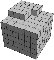
Figure 1: A configuration of the reference path.

From the results of Neves N2 , N1 and a direct computation, we derive the following facts. Let

$$l_{c}(d)=\biggl{\lfloor}\frac{2(d-1)}{h}\biggr{\rfloor}.$$

The configuration of volume $m_{d}$ is a quasicube with sides of length $l_{c}(d)$ or $l_{c}(d)+1$, with a $(d-1)$-dimensional critical droplet attached on one of its largest sides. The precise shape of the critical droplet depends on the value of $h$ (see, e.g., BAC for $d=3$); by the precise shape, we mean the number of sides of the quasicube which are equal to $l_{c}(d)$ and $l_{c}(d)+1$. It is possible to derive exact formulas for $m_{d}$ and ${\Gamma}_{d}$, but they are complicated, and it is necessary to consider various cases according to the value of $h$. However, we have $m_{1}=1$, ${\Gamma}_{1}=2-h$ and the following inequalities

$$\bigl{(}l_{c}(d)\bigr{)}^{d} \leq m_{d}\leq\bigl{(}l_{c}(d)+1\bigr{)}^{d},$$

$$2d\bigl{(}l_{c}(d)\bigr{)}^{d-1}-h\bigl{(}l_{c}(d)+1\bigr{)}^{d} \leq \Gamma_{d}\leq 2d\bigl{(}l_{c}(d)+1\bigr{)}^{d-1}-h\bigl{(}l_{c}(d)\bigr{)}^{d}.$$

This yields the following expansions as $h$ goes to $0$:

$$m_{d}\sim\biggl{(}\frac{2(d-1)}{h}\biggr{)}^{d},\qquad{\Gamma}_{d}\sim 2\biggl{(}\frac{2(d-1)}{h}\biggr{)}^{d-1}.$$

Lemma 4.1

The energy $\Gamma_{d}$ of the critical droplet in dimension $d$ is a continuous function of the magnetic field $h$.

Let $h_{0}>0$. Let ${\Lambda}$ be a box of side length larger than $4d/h_{0}$. From the previous results, for any $h\geq h_{0}$, we have the equality

$$\Gamma_{d}=\max_{0\leq k\leq|\Lambda|}\min\bigl{\{}H(\sigma)\dvtx\sigma\in\{-1,+1\}^{\Lambda},|\sigma|=k\bigr{\}}.$$

Given a configuration $\sigma$ of spins in $\Lambda$, the Hamiltonian $H(\sigma)$ is a continuous function of the magnetic field $h$. For $k\leq|\Lambda|$, the number of configurations $\sigma$ such that $|\sigma|=k$ is finite, thus the minimum

$$\min\bigl{\{}H(\sigma)\dvtx\sigma\in\{-1,+1\}^{\Lambda},|\sigma|=k\bigr{\}}$$

is also a continuous function of $h$. Thus $\Gamma_{d}$ is also a continuous function of $h$ on $[h_{0},+\infty[$. This holds for any $h_{0}>0$, thus $\Gamma_{d}$ is a continuous function of $h$ on $]0,+\infty[$.

Our next goal is to prove that the maximal depth of the cycles in a reference cycle path is smaller than ${\Gamma}_{d-1}$. Let $\rho=(\rho_{0},\ldots,\rho_{|{\Lambda}|})$ be a reference path, and let $(\pi_{0},\ldots,\pi_{|{\Lambda}|})$ be the corresponding reference cycle path. We set

$$\Delta_{d}=\max_{0\leq i<m_{d}}0pt(\pi_{i})=\max_{0\leq i<m_{d}}\bigl{(}E(\pi_{i},\mathbf{-1})-E\bigl{(}\operatorname{bottom}(\pi_{i})\bigr{)}\bigr{)}.$$

Proposition 4.2

The maximal depth $\Delta_{d}$ of the cycles in a reference cycle path is strictly less than ${\Gamma}_{d-1}$.

For $i<m_{d}$ the configuration $\rho_{i}$ belongs to ${\cal C}_{d}$, and we have

$$E(\pi_{i},\mathbf{-1})=\max_{0\leq j\leq i}H(\rho_{j}).$$

Let us define, for $0\leq i\leq r$,

$$\underline{v}_{i} = \min\bigl{\{}|\sigma|\dvtx\sigma\in\pi_{i}\bigr{\}},$$

$$\overline{v}_{i} = \max\bigl{\{}|\sigma|\dvtx\sigma\in\pi_{i}\bigr{\}}.$$

Whenever $i<m_{d}$, the value $\underline{v}_{i}$ is the unique integer $v$ such that

$$H(\rho_{v-1})=E(\pi_{i},\mathbf{-1}).$$

Thanks to the minimax property of the reference path, we have also that $\rho_{k}\in\pi_{i}$ for $\underline{v}_{i}\leq k\leq\overline{v}_{i}$ whence

$$E\bigl{(}\operatorname{bottom}(\pi_{i})\bigr{)}=\min\bigl{\{}H(\rho_{k})\dvtx\underline{v}_{i}\leq k\leq\overline{v}_{i}\bigr{\}}.$$

From the previous identities, we infer that

$$\Delta_{d} = \max_{0\leq i<m_{d}}\max\bigl{\{}H(\rho_{\underline{v}_{i}-1})-H(\rho_{k})\dvtx\underline{v}_{i}\leq k\leq\overline{v}_{i}\bigr{\}}$$

$$\leq \max_{0\leq j\leq i<m_{d}}\bigl{(}H(\rho_{j})-H(\rho_{i})\bigr{)}.$$

The maximum of the energy along a $(d-1)$-dimensional reference path is reached at the value $m_{d-1}$, while the minimum of the energy is reached at one of the two ends of the path. Therefore the indices $i^{*},j^{*}$ realizing the maximum of the right-hand side correspond, respectively, to a quasicube $\rho_{i^{*}}$ and the union $\rho_{j^{*}}$ of a quasicube $c^{*}$ and a $(d-1)$-dimensional critical droplet. Since $j^{*}\leq i^{*}$, we have $c^{*}\subset\rho_{j^{*}}\subset\rho_{i^{*}}$. The quasicubes $c^{*}$ and $\rho_{i^{*}}$ being subcritical, we have $H(c^{*})<H(\rho_{i^{*}})$ and therefore

$$\Delta_{d}\leq H(\rho_{j^{*}})-H(\rho_{i^{*}})<H(\rho_{j^{*}})-H\bigl{(}{c^{*}}\bigr{)}\leq{\Gamma}_{d-1}.$$

The last inequality holds also when $c^{*}$ is too small so that a $(d-1)$-dimensional critical droplet cannot be attached to one of its faces.

4.4 Boxes with $n\pm$ boundary conditions

Unlike in the simplified model studied in CM2 , we cannot use here a direct induction on the dimension $d$. Instead, we introduce special boundary conditions that make a $d$-dimensional system behave like a $n$-dimensional system. For $E$ a subset of ${\mathbb{Z}}^{d}$, we define its outer vertex boundary $\partial^{\mathrm{out}}E$ as

$$\partial^{\mathrm{out}}E=\bigl{\{}x\in{\mathbb{Z}}^{d}\setminus E\dvtx\exists y\in E,|y-x|=1\bigr{\}}.$$

Let $n\in\{0,\ldots,d\}$. We define next mixed boundary conditions for parallelepipeds with minus on $2n$ faces and plus on $2d-2n$ faces.

$n\pm$ Boundary condition. Let $R$ be a parallelepiped. We write $R$ as the product $R=\Lambda_{1}\times\Lambda_{2}$, where $\Lambda_{1},\Lambda_{2}$ are parallelepipeds of dimensions $n,d-n$, respectively. We consider the boundary conditions on $R$ defined as:

$\bullet$ minus on $(\partial^{\mathrm{out}}{\Lambda}_{1})\times{\Lambda}_{2}$;

$\bullet$ plus on ${\Lambda}_{1}\times\partial^{\mathrm{out}}{\Lambda}_{2}$.

We denote by $n\pm$ this boundary condition, and by $H^{n\pm}$ the corresponding Hamiltonian in $R$. The $n\pm$ boundary condition on $R$ is obtained by putting minuses on the exterior faces of $R$ orthogonal to the first $n$ axis and pluses on the remaining faces.

Figure 2: $n\pm$ boundary conditions.

We will now transfer the isoperimetric results in ${\mathbb{Z}}^{d}$ to parallelepipeds with $n\pm$ boundary condition.

Lemma 4.3

Let $n\in\{1,\ldots,d\}$. Let $R$ be a $d$-dimensional parallelepiped, and let $l$ be the length of its smallest side. For any configuration $\sigma$ in $R$ such that $|\sigma|<l$, there exists an $n$-dimensional configuration $\rho$ such that

$$|\rho|=|{\sigma}|,\qquad H_{{\mathbb{Z}}^{n}}(\rho)\leq H^{n\pm}_{R}(\sigma).$$

The constraint on the cardinality of $\sigma$ ensures that there is no cluster of pluses connecting two opposite faces of $R$. We endow ${\mathbb{N}}^{d}$ with $n\pm$ boundary conditions by putting minuses on

$$\bigl{(}\{-1\}\times{\mathbb{N}}^{d-1}\bigr{)}\cup\cdots\cup\bigl{(}{\mathbb{N}}^{n-1}\times\{-1\}\times{\mathbb{N}}^{d-n}\bigr{)}$$

and pluses on

$$\bigl{(}{\mathbb{N}}^{n}\times\{-1\}\times{\mathbb{N}}^{d-n-1}\bigr{)}\cup\cdots\cup\bigl{(}{\mathbb{N}}^{d-1}\times\{-1\}\bigr{)}.$$

We shall prove the following assertion, which implies the claim of the lemma. Suppose $n<d$. For any finite configuration $\sigma$ in ${\mathbb{N}}^{d}$, there exists a configuration $\rho$ in ${\mathbb{N}}^{d-1}$ such that

$$|\rho|=|{\sigma}|,\qquad H_{{\mathbb{N}}^{d-1}}^{n\pm}(\rho)\leq H_{{\mathbb{N}}^{d}}^{n\pm}(\sigma).$$

If we start with a configuration $\sigma$ in $R$ such that $|\sigma|<l$, then we apply iteratively this result to the connected components of $\sigma$ (since no connected component of $\sigma$ intersects two opposite faces of $R$, up to a rotation, their energies can be computed as if they were in ${\mathbb{N}}^{d}$ with $n\pm$ boundary conditions). We end up with a configuration $\eta$ in ${\mathbb{N}}^{n}$ with $n\pm$ boundary conditions which satisfies the conclusion of the lemma. We prove next the assertion. Let $\sigma$ be a finite configuration in ${\mathbb{N}}^{d}$, and let $c$ be the polyomino associated to $\sigma$. We let $c$ fall by gravity along the $(n+1)$th axis on ${\mathbb{N}}^{n}\times\{-1\}\times{\mathbb{N}}^{d-n-1}$.

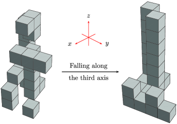
Figure 3: The falling operation.

The resulting polyomino ${\widetilde{c}}$ has the same volume as $c$ and moreover

$$\operatorname{perimeter}({\widetilde{c}})\leq\operatorname{perimeter}(c),$$

because the number of contacts between the unit cubes or with the boundary condition cannot decrease through the “falling” operation. We can think of ${\widetilde{c}}$ as a stack of $(d-1)$-dimensional polyominoes $c_{0},\ldots,c_{k}$, which are obtained by intersecting ${\widetilde{c}}$ with the layers

$$L_{i}=\bigl{\{}x=(x_{1},\ldots,x_{d})\in{\mathbb{N}}^{d}\dvtx i-\tfrac{1}{2}\leq x_{n+1}<i+\tfrac{1}{2}\bigr{\}},\qquad i\in{\mathbb{N}}.$$

Since we have let $c$ fall by gravity to obtain ${\widetilde{c}}$, this stack is nonincreasing in the following sense: for $i$ in ${\mathbb{N}}$, the $(d-1)$-dimensional polyomino $c_{i}$ associated with the layer $L_{i}$ contains the $(d-1)$-dimensional polyomino $c_{i+1}$ associated with the layer $L_{i+1}$. As a consequence,

$$H_{{\mathbb{N}}^{d}}^{n\pm}({\widetilde{c}})\geq\sum_{i\geq 0}H_{{\mathbb{N}}^{d-1}}^{n\pm}(c_{i})+\operatorname{area}\bigl{(}\mathrm{proj}_{n+1}({\widetilde{c}})\bigr{)},$$

where $\mathrm{proj}_{n+1}({\widetilde{c}})$ is the orthogonal projection of ${\widetilde{c}}$ on ${\mathbb{N}}^{n}\times\{-1\}\times{\mathbb{N}}^{d-n-1}$. Let ${\widehat{c}}$ be a $(d-1)$-dimensional polyomino obtained as the union of disjoint translates of $c_{0},\ldots,c_{k}$. The polyomino ${\widehat{c}}$ answers the problem.

Let ${\Lambda}$ be a box whose sides are larger than $m_{n}$. We construct next a reference path $(\rho^{n\pm}_{i},0\leq i\leq|{\Lambda}|)$ in the box ${\Lambda}$ endowed with $n\pm$ boundary conditions with the following algorithm: [(4)]

Compute the maximum number $m$ of plus neighbors for a minus site in the box (taking into account the boundary conditions).

If there is only one site realizing this maximum, put a plus at this site and go to step 1.

Otherwise, compute the maximal length of a segment of minus sites having all $m$ plus neighbors.

Put a plus at a site of a segment realizing the previous maximum and go to step 1. As before, the reference path $(\rho^{n\pm}_{i},0\leq i\leq|{\Lambda}|)$ realizes the solution of the minimax problem associated with the communication energy between any two of its configurations. The metastable cycle ${\cal C}_{d}^{n\pm}$ in the box $\Lambda$ with $n\pm$ boundary conditions is the maximal cycle of

$$\{-1,+1\}^{\Lambda}\setminus\{\mathbf{-1},\mathbf{+1}\}$$

containing $\mathbf{-1}$ in the energy landscape associated to the Hamiltonian $H^{n\pm}_{{\Lambda}}$.

Corollary 4.4.

The depth of the metastable cycle ${\cal C}_{d}^{n\pm}$ is equal to ${\Gamma}_{n}$.

With the help of Lemma 4.3, we can compare the energy along a path in ${\Lambda}$ with $n\pm$ boundary conditions with the energy along a path in ${\mathbb{Z}}^{n}$, in such a way that at each index the configurations in each path have the same cardinality. This construction implies immediately that

$$0pt\bigl{(}{\cal C}_{d}^{n\pm}\bigr{)}\geq{\Gamma}_{n}.$$

To get the converse inequality we simply consider the reference path in ${\Lambda}$ with $n\pm$ boundary conditions.

Corollary 4.5.

The maximal depth $\Delta_{d}^{n\pm}$ of the cycles in a reference cycle path with $n\pm$ boundary conditions is strictly less than ${\Gamma}_{n-1}$.

We check that, until the index $m_{n}$, the energy along the reference path $(\rho^{n\pm}_{i},i\geq 0)$ is equal to the energy along the reference path in ${\mathbb{Z}}^{n}$ computed with $H_{{\mathbb{Z}}^{n}}$. The result follows then from Proposition 4.2.

5 The space–time clusters

The goal of this section is to prove Theorem 5.7, which provides a control on the diameter of the space–time clusters. Theorem 5.7 is used in an essential way in the proof of the lower bound on the relaxation time, under the following weaker form: for the dynamics restricted to a small box, the probability of creating a large $\operatorname{\mbox{{stc}}}$ before nucleation is SES. We first recall the basic definitions and properties of the space–time clusters in Section 5.1. We next proceed to show that it is very unlikely that large space–time clusters are formed before nucleation. The main theorem of this section, Theorem 5.7, is the analog of Lemma 4 in DS1 . The proof in DS1 relies on the fact that in two dimensions the energy needed to grow, that is, the energy of a protuberance, is larger than the energy needed to shrink a subcritical droplet. In higher dimension, we are not able to prove a corresponding result. Let us give a quick sketch of the proof of Theorem 5.7. We consider a set ${\cal D}$ satisfying a technical hypothesis, and we want to control the probability of creating a large space–time cluster before exiting ${\cal D}$. Typically, the set ${\cal D}$ is a cycle or a cycle compound included in the metastable cycle. We use several ideas coming from the theory of simulated annealing CaCe . We decompose ${\cal D}$ into its maximal cycle compounds, and we show that, before exiting ${\cal D}$, the process is unlikely to make a large number of jumps between these maximal cycle compounds. Thus, if a large space–time cluster is created, then it must be created during a visit to a maximal cycle compound. The problem is therefore reduced to control the size of the space–time cluster created inside a cycle compound $\overline{\cal A}$ included in ${\cal D}$. The key estimate is proved by induction over the depth of the cycle compound. Suppose we want to prove the estimate for a cycle compound $\overline{\cal A}$. A first key fact, proved in Lemma 5.4 with the help of the ferromagnetic inequality, is that in the Ising model under irrational magnetic field the bottom of every cycle compound is a singleton. Let $\eta$ be the bottom of the cycle compound $\overline{\cal A}$. We consider now the trajectory of the process starting from a point of $\overline{\cal A}$ until it exits from $\overline{\cal A}$. In Section 5.4, in order to control the size of the space–time clusters, we define a quantity $\operatorname{diam}_{\infty}\operatorname{\mbox{{stc}}}(s,t)$ depending on a time interval $[s,t]$. This quantity is larger than the increase of the maximum of the diameters of the space–time clusters created between the times $s$ and $t$. Moreover this quantity is subadditive with respect to the time; see Lemma 5.6. Our strategy is to look at the successive visits to $\eta$ and the excursions outside of $\eta$. Suppose that $\eta$ has only one connected component. The creation of a large space–time cluster in a fixed direction has to be achieved during an excursion outside of $\eta$. Indeed, each time the process comes back to $\eta$, the growth of the space–time clusters restarts almost from scratch.

Thus if a large space–time cluster is created before the exit of $\overline{\cal A}$, then it has to be created during an excursion outside of $\eta$. The situation is more complicated when the bottom $\eta$ has several connected components. Indeed, the space–time clusters associated to one connected component might change between two consecutive visits to $\eta$. We prove in Section 5.3 that this does not happen: at each visit to $\eta$, a given connected component of $\eta$ always belong to the same space–time cluster. This is a consequence of Lemma 5.5. Figure 4 shows an example of the space–time clusters associated to a configuration $\eta$ having two connected components. On the evolution depicted in the figure, the space–time clusters containing the lower component of $\eta$ at the times of the first two returns are distinct. We will prove that this cannot occur as long as the process stays in the cycle compound $\overline{\cal A}$ (this is the purpose of Lemma 5.5).

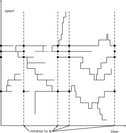
Figure 4: Evolution of a STC in dimension 1.

We rely then on a technique going back to the theory of simulated annealing, which consists of removing the bottom $\eta$ from $\overline{\cal A}$, decomposing $\overline{\cal A}\setminus\{\eta\}$ into its maximal cycle compounds and studying the jumps of the process between these maximal cycle compounds until the exit of $\overline{\cal A}\setminus\{\eta\}$. As before, we show that, before exiting $\overline{\cal A}\setminus\{\eta\}$, the process is unlikely to make a large number of jumps between these maximal cycle compounds. This step is very similar to the initial step, when we considered a general set ${\cal D}$. For the clarity of the exposition, we prefer to repeat the argument rather than to introduce additional notation and make a general statement. Using the subadditivity of $\operatorname{diam}_{\infty}\operatorname{\mbox{{stc}}}(s,t)$, we conclude that a large space–time cluster has to be created during a visit to a maximal cycle compound of $\overline{\cal A}\setminus\{\eta\}$. Now each cycle compound included in $\overline{\cal A}\setminus\{\eta\}$ has a depth strictly smaller than the depth of $\overline{\cal A}$. Using the induction hypothesis, we have a control on the space–time clusters created during each visit to these cycle compounds. Combining the estimate provided by the induction hypothesis and the estimate on the number of cycle compounds of $\overline{\cal A}\setminus\{\eta\}$ visited by the process, we obtain a control on the size of the space–time clusters created during an excursion in $\overline{\cal A}\setminus\{\eta\}$. Using the estimates presented in Section 2.3, we can also control the number of visits to $\eta$ before the exit of $\overline{\cal A}$. The induction step is completed by combining all the previous estimates.

5.1 Basic definitions and properties

Let $\Lambda$ be a subset of ${\mathbb{Z}}^{d}$ and let $(\sigma_{{\Lambda},t})_{t\geq 0}$ be a continuous-time trajectory in $\{-1,+1\}^{\Lambda}$. We endow the set of the space–time points $\Lambda\times{\mathbb{R}}^{+}$ with the following connectivity relation: the two space–time points $(x,t)$ and $(y,s)$ are connected if $\sigma_{{\Lambda},t}(x)=\sigma_{{\Lambda},s}(y)=+1$ and:

$\bullet$ either $s=t$ and $|x-y|\leq 1$;

$\bullet$ or $x=y$ and $\sigma_{{\Lambda},u}(x)=+1$ for $u\in[\min(s,t),\max(s,t)]$.

A space–time cluster of the trajectory $(\sigma_{{\Lambda},t})_{t\geq 0}$ is a maximal connected component of space–time points. For $u\leq s\in{\mathbb{R}}^{+}$, we denote by $\operatorname{\mbox{{stc}}}(u,s)$ the space–time clusters of the trajectory restricted to the time interval $[u,s]$. Sometimes we deal with a specific initial condition $\alpha$ and boundary conditions ${\zeta}$. We denote by $\operatorname{\mbox{{stc}}}({\sigma}^{\alpha,{\zeta}}_{{\Lambda},t},s\leq t\leq u)$ the space–time clusters of the trajectory of the process $({\sigma}^{\alpha,{\zeta}}_{{\Lambda},t})_{t\geq 0}$ restricted to the time interval $[u,s]$.

The graphical construction updates the configuration in two different places independently until a space–time cluster connects the two places. We state next a refinement of Lemma 2 of DS1 , which allows us to compare processes defined in different volumes or with different boundary conditions via the graphical construction described in Section 3.2.

Lemma 5.1

Let ${\Lambda}$ be a subset of ${\mathbb{Z}}^{d}$, and let ${\zeta}$ be a boundary condition on ${\Lambda}$. Let $x$ be a site of the exterior boundary of ${\Lambda}$ such that ${\zeta}(x)=+1$. If ${\cal C}$ is a $\operatorname{\mbox{{stc}}}$ for the dynamics in ${\Lambda}$ with ${\zeta}$ as boundary conditions, and ${\cal C}$ is such that $x$ is not the neighbor of a point of ${\cal C}$, then ${\cal C}$ is also a $\operatorname{\mbox{{stc}}}$ for the dynamics in ${\Lambda}$ with ${\zeta}^{x}$ as boundary conditions.

We denote by $\alpha$ the initial configuration. From the coupling, we have

$$\forall t\geq 0,\forall y\in{\Lambda}\qquad{\sigma}^{\alpha,{\zeta}^{x}}_{{\Lambda},t}(y)\leq{\sigma}^{\alpha,{\zeta}}_{{\Lambda},t}(y).$$

Let ${\cal C}$ be a $\operatorname{\mbox{{stc}}}$ in $\operatorname{\mbox{{stc}}}({\sigma}^{\alpha,{\zeta}}_{{\Lambda},t},s\leq t\leq u)$ and suppose that ${\cal C}$ does not belong to $\operatorname{\mbox{{stc}}}({\sigma}^{\alpha,{\zeta}^{x}}_{{\Lambda},t},s\leq t\leq u)$. Necessarily, there exists a space–time point $(y,t)$ such that

$$(y,t)\in{\cal C},\qquad{\sigma}^{\alpha,{\zeta}^{x}}_{{\Lambda},t}(y)=-1,\qquad{\sigma}^{\alpha,{\zeta}}_{{\Lambda},t}(y)=+1.$$

We consider the set of the space–time points satisfying the above condition, and we denote by $(y^{*},t^{*})$ the space–time point such that $t^{*}$ is minimum. This is possible since the number of spin flips in a finite box is finite in a finite time interval, and moreover the trajectories are right continuous. At time $t^{*}$, the spin at site $y^{*}$ becomes $+1$ in the process $({\sigma}^{\alpha,{\zeta}}_{{\Lambda},t})_{t\geq 0}$, and it remains equal to $-1$ in $({\sigma}^{\alpha,{\zeta}^{x}}_{{\Lambda},t})_{t\geq 0}$. We examine next the neighbors of $y^{*}$. Let $z$ be a neighbor of $y^{*}$ in ${\Lambda}$. If ${\sigma}^{\alpha,{\zeta}}_{{\Lambda},t^{*}}(z)=-1$, then ${\sigma}^{\alpha,{\zeta}^{x}}_{{\Lambda},t^{*}}(z)=-1$ as well. Suppose that ${\sigma}^{\alpha,{\zeta}}_{{\Lambda},t^{*}}(z)=+1$. The spin at $z$ does not change at time $t^{*}$, thus for $s<t^{*}$ close enough to $t^{*}$, we have also ${\sigma}^{\alpha,{\zeta}}_{{\Lambda},s}(z)=+1$. This implies that $\{z\}\times[s,t^{*}]$ is included in ${\cal C}$. From the definition of $(y^{*},t^{*})$, we have that

$$\forall u\in\bigl{[}s,t^{*}\bigr{]}\qquad{\sigma}^{\alpha,{\zeta}^{x}}_{{\Lambda},u}(z)=+1.$$

We conclude that the neighbors of $y^{*}$ in ${\Lambda}$ have the same spins in ${\sigma}^{\alpha,{\zeta}^{x}}_{{\Lambda},t^{*}}$ and in ${\sigma}^{\alpha,{\zeta}}_{{\Lambda},t^{*}}$. Therefore $y^{*}$ must have a neighbor in ${\mathbb{Z}}^{d}\setminus{\Lambda}$ whose spin is different in ${\sigma}^{\alpha,{\zeta}^{x}}_{{\Lambda},t^{*}}$ and in ${\sigma}^{\alpha,{\zeta}}_{{\Lambda},t^{*}}$. The only possible candidate is $x$.

The next corollary is very close to Lemma 2 of DS1 .

Corollary 5.2.

Let ${\Lambda}_{1}\subset{\Lambda}_{2}$ be two subsets of ${\mathbb{Z}}^{d}$, let $\alpha$ be an initial configuration in ${\Lambda}_{2}$ and let ${\zeta}$ be a boundary condition on ${\Lambda}_{2}$. If no $\operatorname{\mbox{{stc}}}$ of the process $({\sigma}^{\alpha,{\zeta}}_{{\Lambda}_{2},t},s\leq t\leq u)$ intersects both ${\Lambda}_{1}$ and the inner boundary of ${\Lambda}_{2}$, then

$$\forall t\in[s,u]\qquad{\sigma}^{\alpha,{\zeta}}_{{\Lambda}_{2},t}|_{{\Lambda}_{1}}={\sigma}^{\alpha,-}_{{\Lambda}_{2},t}|_{{\Lambda}_{1}}.$$

We define the diameter $\operatorname{diam}_{\infty}{\cal C}$ of a space–time cluster ${\cal C}$ by

$$\operatorname{diam}_{\infty}{\cal C}=\sup\bigl{\{}|x-y|_{\infty}\dvtx(x,s),(y,t)\in{\cal C}\bigr{\}},$$

where $|\cdot|_{\infty}$ is the supremum norm given by

$$\forall x=(x_{1},\ldots,x_{d})\in{\mathbb{Z}}^{d}\qquad|x|_{\infty}=\max_{1\leq i\leq d}|x_{i}|.$$

Thus $\operatorname{diam}_{\infty}{\cal C}$ is the diameter of the spatial projection of ${\cal C}$.

5.2 The bottom of a cycle compound

We prove here that, when $h$ is irrational, the bottom of a cycle compound of the Ising model contains a unique configuration. Throughout the section, we consider a finite box $Q$ endowed with a boundary condition $\xi$. To alleviate the formulas, we write simply $H$ instead of $H_{Q}^{\xi}$.

Lemma 5.3

Suppose that $h$ is irrational. Let ${\eta}$ be a minimizer of the energy in a cycle compound $\overline{{\cal A}}$. Then for any ${\zeta}\in\overline{{\cal A}}$, ${\zeta}\cup{\eta}\in\overline{{\cal A}}$ and ${\zeta}\cap{\eta}\in\overline{{\cal A}}$.

Let $\eta$ belong to the bottom of $\overline{\cal A}$. We assume that $\overline{{\cal A}}$ is not a singleton; otherwise there is nothing to prove. Let ${\omega}=({\omega}_{1},\ldots,{\omega}_{n})$ be a path in $\overline{{\cal A}}$ that goes from ${\eta}$ to ${\zeta}$. We associate with ${\omega}$ a slim path

$${\omega}\cap\eta=({\omega}_{1}\cap{\eta},\ldots,{\omega}_{n}\cap{\eta})$$

and a fat path

$${\omega}\cup\eta=({\omega}_{1}\cup{\eta},\ldots,{\omega}_{n}\cup{\eta}).$$

Suppose that the thesis is false, and let us set

$${\kappa}^{*}=\min\{k\geq 1\dvtx{\omega}_{k}\cap{\eta}\notin\overline{{\cal A}}\mbox{ or }{\omega}_{k}\cup{\eta}\notin\overline{{\cal A}}\}.$$

Notice that ${\kappa}^{*}$ is larger than or equal to $2$. We will use the attractive inequality

$$H({\omega}_{k}\cap{\eta})+H({\omega}_{k}\cup{\eta})\leq H({\omega}_{k})+H({\eta})$$

and the fact that ${\eta}$ is a minimizer of the energy in $\overline{{\cal A}}$. Let us set

$$\lambda=E\bigl{(}\overline{{\cal A}},\{-1,+1\}^{{\Lambda}}\setminus\overline{{\cal A}}\bigr{)}.$$

First, for any $k<{\kappa}^{*}$, the above inequality yields that

$$\max\bigl{(}H({\omega}_{k}\cap{\eta}),H({\omega}_{k}\cup{\eta})\bigr{)}\leq H({\omega}_{k})\leq\lambda.$$

The configurations ${\omega}_{{\kappa}^{*}}$ and ${\omega}_{{\kappa}^{*}-1}$ differ for the spin in a single site. We say that the ${\kappa}^{*}$th spin flip is inside (resp., outside) ${\eta}$ if this site has a plus spin (resp., a minus spin) in ${\eta}$, that is, if ${\omega}_{{\kappa}^{*}}\vartriangle{\omega}_{{{\kappa}^{*}}-1}\subset{\eta}$ (resp., ${\omega}_{{\kappa}^{*}}\vartriangle{\omega}_{{{\kappa}^{*}}-1}\not\subset{\eta}$). We distinguish two cases, according to the position of the ${\kappa}^{*}$th spin flip with respect to ${\eta}$:

(i) if the ${\kappa}^{*}$th spin flip is inside ${\eta}$, then ${\omega}_{{\kappa}^{*}}\cup{\eta}={\omega}_{{\kappa}^{*}-1}\cup{\eta}$, so that only the slim path moves and exits $\overline{\cal A}$ at index ${\kappa}^{*}$. Thus

$${\omega}_{{\kappa}^{*}-1}\cap{\eta}\in\overline{\cal A},\qquad{\omega}_{{\kappa}^{*}}\cap{\eta}\notin\overline{\cal A}$$

and these two configurations communicate, therefore

$$\max\bigl{(}H({\omega}_{{\kappa}^{*}-1}\cap{\eta}),H({\omega}_{{\kappa}^{*}}\cap{\eta})\bigr{)}\geq\lambda.$$

We distinguish again two cases:

$\bullet$ $H({\omega}_{{\kappa}^{*}-1}\cap{\eta})\geq\lambda$. Since $H({\omega}_{{\kappa}^{*}-1}\cap{\eta})\leq H({\omega}_{{\kappa}^{*}-1})\leq\lambda$, then ${\omega}_{{\kappa}^{*}-1}\cap{\eta}$ and ${\omega}_{{\kappa}^{*}-1}$ have both an energy equal to $\lambda$, and by Lemma 3.1, we conclude that ${\omega}_{{\kappa}^{*}-1}\cap{\eta}={\omega}_{{\kappa}^{*}-1}$ and ${\omega}_{{\kappa}^{*}-1}$ is included in ${\eta}$. Since we are assuming that the slim path moves at step ${\kappa}^{*}$, the original path and the slim path undergo the same spin flip so that they must coincide also at step ${\kappa}^{*}$, contradicting the assumption that ${\omega}_{{\kappa}^{*}}\cap{\eta}\notin\overline{{\cal A}}$.

$\bullet$ $H({\omega}_{{\kappa}^{*}}\cap{\eta})\geq\lambda$. By the attractive inequality

$$H({\omega}_{{\kappa}^{*}})-H({\omega}_{{\kappa}^{*}}\cap{\eta})\geq H({\omega}_{{\kappa}^{*}-1}\cup{\eta})-H({\eta})\geq 0,$$

whence

$$H({\omega}_{{\kappa}^{*}}\cap{\eta})\leq H({\omega}_{{\kappa}^{*}})\leq\lambda.$$

Thus ${\omega}_{{\kappa}^{*}}\cap{\eta}$ and ${\omega}_{{\kappa}^{*}}$ have both an energy equal to $\lambda$. By Lemma 3.1, we conclude that ${\omega}_{{\kappa}^{*}}\cap{\eta}={\omega}_{{\kappa}^{*}}$, contradicting the assumption that ${\omega}_{{\kappa}^{*}}\cap{\eta}\notin\overline{{\cal A}}$.

We consider next the second case. The argument is very similar in the two dual cases (i) and (ii), yet it seems necessary to handle them separately.

(ii) if the ${\kappa}^{*}$th spin flip is outside ${\eta}$, then ${\omega}_{{\kappa}^{*}}\cap{\eta}={\omega}_{{\kappa}^{*}-1}\cap{\eta}$, so that only the fat path moves and exits $\overline{\cal A}$ at index ${\kappa}^{*}$. Thus

$${\omega}_{{\kappa}^{*}-1}\cup{\eta}\in\overline{\cal A},\qquad{\omega}_{{\kappa}^{*}}\cup{\eta}\notin\overline{\cal A}$$

and these two configurations communicates, therefore

$$\max\bigl{(}H({\omega}_{{\kappa}^{*}-1}\cup{\eta}),H({\omega}_{{\kappa}^{*}}\cup{\eta})\bigr{)}\geq\lambda.$$

We distinguish again two cases:

$\bullet$ $H({\omega}_{{\kappa}^{*}-1}\cup{\eta})\geq\lambda$. Since $H({\omega}_{{\kappa}^{*}-1}\cup{\eta})\leq H({\omega}_{{\kappa}^{*}-1})\leq\lambda$, then ${\omega}_{{\kappa}^{*}-1}\cup{\eta}$ and ${\omega}_{{\kappa}^{*}-1}$ have both an energy equal to $\lambda$, and by Lemma 3.1, we conclude that ${\omega}_{{\kappa}^{*}-1}\cup{\eta}={\omega}_{{\kappa}^{*}-1}$ and ${\omega}_{{\kappa}^{*}-1}$ contains ${\eta}$. Since we are assuming that the fat path moves at step ${\kappa}^{*}$, the original path and the fat path undergo the same spin flip so that they must coincide also at step ${\kappa}^{*}$, contradicting the assumption that ${\omega}_{{\kappa}^{*}}\cup{\eta}\notin\overline{{\cal A}}$.

$\bullet$ $H({\omega}_{{\kappa}^{*}}\cup{\eta})\geq\lambda$. By the attractive inequality

$$H({\omega}_{{\kappa}^{*}})-H({\omega}_{{\kappa}^{*}}\cup{\eta})\geq H({\omega}_{{\kappa}^{*}-1}\cap{\eta})-H({\eta})\geq 0,$$

whence

$$H({\omega}_{{\kappa}^{*}}\cup{\eta})\leq H({\omega}_{{\kappa}^{*}})\leq\lambda.$$

Thus ${\omega}_{{\kappa}^{*}}\cup{\eta}$ and ${\omega}_{{\kappa}^{*}}$ have both an energy equal to $\lambda$. By Lemma 3.1, we conclude that ${\omega}_{{\kappa}^{*}}\cup{\eta}={\omega}_{{\kappa}^{*}}$, contradicting the assumption that ${\omega}_{{\kappa}^{*}}\cup{\eta}\notin\overline{{\cal A}}$.

Lemma 5.4

Suppose that $h$ is irrational. The bottom $\operatorname{bottom}(\overline{{\cal A}})$ of any cycle compound $\overline{{\cal A}}$ contains a single configuration.

If ${\eta}_{1},{\eta}_{2}\in\operatorname{bottom}(\overline{{\cal A}})$, then by Lemma 5.3 we have also ${\eta}_{1}\cup{\eta}_{2}\in\overline{{\cal A}}$ and ${\eta}_{1}\cap{\eta}_{2}\in\overline{{\cal A}}$, so that $H({\eta}_{1})+H({\eta}_{2})\leq H({\eta}_{1}\cup{\eta}_{2})+H({\eta}_{1}\cap{\eta}_{2})$. But by the attractive inequality,

$$H({\eta}_{1}\cup{\eta}_{2})+H({\eta}_{1}\cap{\eta}_{2})\leq H({\eta}_{1})+H({\eta}_{2}),$$

so that ${\eta}_{1}\cup{\eta}_{2}$ and ${\eta}_{1}\cap{\eta}_{2}$ are also in $\operatorname{bottom}(\overline{{\cal A}})$. Lemma 3.1 implies that ${\eta}_{1}\cup{\eta}_{2}={\eta}_{1}\cap{\eta}_{2}$, showing that ${\eta}_{1}={\eta}_{2}$.

5.3 The space–time clusters in a cycle compound

In this section, we study some properties of the paths contained in suitable cycle compounds. In order to avoid unnecessary notation, with a slight abuse of terms, we consider space–time clusters associated to a discrete time trajectory. In other words, in this section the word “time” means “index of the configuration in the trajectory,” and the space–time clusters considered here are pure geometrical objects. We will use these geometrical results in order to control the diameter of the space–time clusters of our processes.

As in the previous section, we consider a finite box $Q$ endowed with a boundary condition $\xi$. To alleviate the formulas, we write simply $H$ instead of $H_{Q}^{\xi}$. A connected component of a configuration $\sigma$ is a maximal connected subset of the plus sites of $\sigma$

$$\bigl{\{}x\in{\mathbb{Z}}^{d}\dvtx\sigma(x)=+1\bigr{\}},$$

two sites being connected if they are nearest neighbors on the lattice. We denote by ${\cal C}(\sigma)$ the connected components of $\sigma$. If $C\in{\cal C}(\sigma)$, then we define its energy as

$$H(C)=\bigl{|}\bigl{\{}\{x,y\}\dvtx x\notin C,y\in C,|x-y|=1\bigr{\}}\bigr{|}-h|C|.$$

In particular, we have

$$H(\sigma)=\sum_{C\in{\cal C}(\sigma)}H(C).$$

Let ${\omega}=({\omega}_{0},\ldots,{\omega}_{r})$ be a path of configurations in the box $Q$. We endow the set of the space–time points $Q\times{\mathbb{N}}$ with the following connectivity relation associated to ${\omega}$: the two space–time points $(x,i)$ and $(y,j)$ are connected if ${\omega}_{i}(x)={\omega}_{j}(y)=+1$ and:

$\bullet$ either $i=j$ and $|x-y|\leq 1$;

$\bullet$ or $x=y$ and $|i-j|=1$.

A space–time cluster of the path ${\omega}$ is a maximal connected component of space–time points in ${\omega}$. We consider a domain ${\cal D}$, which is a set of configurations satisfying the following hypothesis.

Hypothesis on ${\cal D}$. The configurations in ${\cal D}$ are such that:

$\bullet$ There exists $v_{\cal D}$ (independent of $\beta$) such that $|\sigma|\leq v_{\cal D}$ for any $\sigma\in{\cal D}$.

$\bullet$ If $\sigma\in{\cal D}$ and $C$ is a connected component of $\sigma$, then we have $H(C)>H(\mathbf{-1})$.

$\bullet$ If $\sigma\in{\cal D}$ and $\eta$ is such that $\eta\subset\sigma$ and $H(\eta)\leq H(\sigma)$, then $\eta\in{\cal D}$.

Lemma 5.5

Let $\overline{{\cal A}}$ be a cycle compound included in ${\cal D}$, and let $\eta$ be the unique configuration of $\operatorname{bottom}(\overline{{\cal A}})$. Let ${\omega}=({\omega}_{0},\ldots,{\omega}_{r})$ be a path in $\overline{{\cal A}}$ starting at $\eta$ and ending at $\eta$. Let $C$ be a connected component of $\eta$. Then the space–time sets $C\times\{0\}$ and $C\times\{r\}$ belong to the same space–time cluster of ${\omega}$.

From Lemma 5.4, we know that $\operatorname{bottom}(\overline{{\cal A}})$ is reduced to a single configuration ${\eta}$. By Lemma 5.3, the path

$${\omega}\cap\eta=({\omega}_{0}\cap{\eta},\ldots,{\omega}_{r}\cap{\eta})$$

is still a path in $\overline{{\cal A}}$ that goes from $\eta$ to $\eta$. Moreover, the space–time clusters of ${\omega}\cap\eta$ are included in those of ${\omega}$, therefore it is enough to prove the result for the path ${\omega}\cap\eta$. Let $\widetilde{\omega}$ be the path obtained from ${\omega}\cap\eta$ by removing all the space–time clusters of ${\omega}\cap\eta$ which do not intersect $\eta\times\{0\}$. The path $\widetilde{\omega}$ is still admissible, that is, it is a sequence of configurations such that each configuration communicates with its successor. Let $i\in\{0,\ldots,r\}$. We have $\widetilde{\omega}_{i}\subset{\omega}_{i}\cap\eta$. Since $\widetilde{\omega}_{i}$ is obtained from ${\omega}_{i}\cap\eta$ by removing some connected components of ${\omega}_{i}\cap\eta$, the second hypothesis on the domain ${\cal D}$ yields that $H(\widetilde{\omega}_{i})\leq H({\omega}_{i}\cap\eta)$. With the help of the third hypothesis on ${\cal D}$, we conclude that $\widetilde{\omega}_{i}$ is in ${\cal D}$. In particular the whole path $\widetilde{\omega}$ stays in ${\cal D}$. Suppose that the path $\widetilde{\omega}$ leaves $\overline{\cal A}$ at some index $i$, so that $\widetilde{\omega}_{i}\neq{\omega}_{i}\cap\eta$. We consider two cases:

$\bullet$ $\widetilde{\omega}_{i-1}={\omega}_{i-1}\cap\eta$. In this case, the spin flip between ${\omega}_{i-1}\cap\eta$ and ${\omega}_{i}\cap\eta$ creates a new STC which does not intersect $\eta\times\{0\}$, hence $\widetilde{\omega}_{i}={\omega}_{i-1}\cap\eta$. This contradicts the fact that $\widetilde{\omega}$ leaves $\overline{\cal A}$ at index $i$.

$\bullet$ $\widetilde{\omega}_{i-1}\neq{\omega}_{i-1}\cap\eta$. Since we have also $\widetilde{\omega}_{i}\neq{\omega}_{i}\cap\eta$, then by Lemma 3.1 we have the strict inequality

$$\max\bigl{(}H(\widetilde{\omega}_{i-1}),H(\widetilde{\omega}_{i})\bigr{)}<\max\bigl{(}H({\omega}_{i-1}\cap\eta),H({\omega}_{i}\cap\eta)\bigr{)}\leq E(\overline{\cal A},{\cal X}\setminus\overline{\cal A}).$$

However, since $\widetilde{\omega}$ leaves $\overline{\cal A}$ at index $i$, we have also

$$\max\bigl{(}H(\widetilde{\omega}_{i-1}),H(\widetilde{\omega}_{i})\bigr{)}\geq E(\overline{\cal A},{\cal X}\setminus\overline{\cal A}),$$

which is absurd. Thus the path $\widetilde{\omega}$ stays also in $\overline{\cal A}$. Since

$$H(\widetilde{\omega}_{r})\leq H({\omega}_{r}\cap\eta),\qquad\widetilde{\omega}_{r}\subset{\omega}_{r}\cap\eta=\eta,$$

we have $\widetilde{\omega}_{r}=\eta$ by Lemma 3.1. The path $\widetilde{\omega}$ is included in $\eta\times\{0,\ldots,r\}$, hence, for any connected component $C$ of $\eta$, the space–time cluster of $\widetilde{\omega}$ containing $C\times\{r\}$ is included in $C\times\{0,\ldots,r\}$, so that its intersection with $\eta\times\{0\}$, which is not empty by construction, must be equal to $C\times\{0\}$.

5.4 Triangle inequality for the diameters of the STCs

In the sequel, we consider a trajectory of the process $({\sigma}_{Q,t},t\geq 0)$ in a finite box $Q$, and we study its space–time clusters. For $s<t$, we define

$$\operatorname{diam}_{\infty}\operatorname{\mbox{{stc}}}(s,t)=\max\biggl{(}\mathop{\sum_{{\cal C}\in\operatorname{\mbox{{stc}}}(s,t)}}_{{\cal C}\cap(Q\times\{s,t\})\neq\varnothing}\operatorname{diam}_{\infty}{\cal C},\mathop{\max_{{\cal C}\in\operatorname{\mbox{{stc}}}(s,t)}}_{{\cal C}\cap(Q\times\{s,t\})=\varnothing}\operatorname{diam}_{\infty}{\cal C}\biggr{)}.$$

The main point of this awkward definition is the following triangle inequality.

Lemma 5.6

For any $s<u<t$, we have

$$\operatorname{diam}_{\infty}\operatorname{\mbox{{stc}}}(s,t)\leq\operatorname{diam}_{\infty}\operatorname{\mbox{{stc}}}(s,u)+\operatorname{diam}_{\infty}\operatorname{\mbox{{stc}}}(u,t).$$

When we look at the restriction to the time intervals $(s,u)$ and $(u,t)$ of a $\operatorname{\mbox{{stc}}}$ in $\operatorname{\mbox{{stc}}}(s,t)$ which is alive at time $u$, this $\operatorname{\mbox{{stc}}}$ splits into several $\operatorname{\mbox{{stc}}}$ belonging to $\operatorname{\mbox{{stc}}}(s,u)\cup\operatorname{\mbox{{stc}}}(u,t)$. Yet the diameter of the initial $\operatorname{\mbox{{stc}}}$ is certainly less than the sum of all the diameters of the $\operatorname{\mbox{{stc}}}$ in $\operatorname{\mbox{{stc}}}(s,u)\cup\operatorname{\mbox{{stc}}}(u,t)$ which are alive at time $u$. The proof is quite tedious; however, since this inequality is fundamental for our argument we provide a detailed verification. First, we have

$$\mathop{\mathop{\sum_{{\cal C}\in\operatorname{\mbox{{stc}}}(s,t)}}_{{{\cal C}\cap(Q\times\{s,t\})\neq\varnothing}}}_{{\cal C}\cap(Q\times\{u\})\neq\varnothing}\operatorname{diam}_{\infty}{\cal C}\leq\mathop{\sum_{{\cal C}\in\operatorname{\mbox{{stc}}}(s,u)}}_{{\cal C}\cap(Q\times\{u\})\neq\varnothing}\operatorname{diam}_{\infty}{\cal C}+\mathop{\sum_{{\cal C}\in\operatorname{\mbox{{stc}}}(u,t)}}_{{\cal C}\cap(Q\times\{u\})\neq\varnothing}\operatorname{diam}_{\infty}{\cal C}.$$

Next, if ${\cal C}\in\operatorname{\mbox{{stc}}}(s,t)$ and ${\cal C}\cap(Q\times\{u\})=\varnothing$, then ${\cal C}\in\operatorname{\mbox{{stc}}}(s,u)\cup\operatorname{\mbox{{stc}}}(u,t)$. Thus

$$\mathop{\mathop{\sum_{{\cal C}\in\operatorname{\mbox{{stc}}}(s,t)}}_{{\cal C}\cap(Q\times\{s,t\})\neq\varnothing}}_{{{\cal C}\cap(Q\times\{u\})=\varnothing}}\operatorname{diam}_{\infty}{\cal C}\leq\mathop{\mathop{\sum_{{\cal C}\in\operatorname{\mbox{{stc}}}(s,u)}}_{{\cal C}\cap(Q\times\{s\})\neq\varnothing}}_{{\cal C}\cap(Q\times\{u\})=\varnothing}\operatorname{diam}_{\infty}{\cal C}+\mathop{\mathop{\sum_{{\cal C}\in\operatorname{\mbox{{stc}}}(u,t)}}_{{\cal C}\cap(Q\times\{u\})=\varnothing}}_{{\cal C}\cap(Q\times\{t\})\neq\varnothing}\operatorname{diam}_{\infty}{\cal C}.$$

Summing the two previous inequalities, we get

$$\mathop{\sum_{{\cal C}\in\operatorname{\mbox{{stc}}}(s,t)}}_{{\cal C}\cap(Q\times\{s,t\})\neq\varnothing}\operatorname{diam}_{\infty}{\cal C} \leq \mathop{\sum_{{\cal C}\in\operatorname{\mbox{{stc}}}(s,u)}}_{{\cal C}\cap(Q\times\{s,u\})\neq\varnothing}\operatorname{diam}_{\infty}{\cal C}+\mathop{\sum_{{\cal C}\in\operatorname{\mbox{{stc}}}(u,t)}}_{{\cal C}\cap(Q\times\{u,t\})\neq\varnothing}\operatorname{diam}_{\infty}{\cal C}$$

$$\leq \operatorname{diam}_{\infty}\operatorname{\mbox{{stc}}}(s,u)+\operatorname{diam}_{\infty}\operatorname{\mbox{{stc}}}(u,t).$$

Moreover, if ${\cal C}\in\operatorname{\mbox{{stc}}}(s,t)$, ${\cal C}\cap(Q\times\{s,t\})=\varnothing$ and ${\cal C}\cap(Q\times\{u\})\neq\varnothing$, then

$$\operatorname{diam}_{\infty}{\cal C}\leq\mathop{\mathop{\sum_{{\cal C}\in\operatorname{\mbox{{stc}}}(s,u)}}_{{\cal C}\cap\bigl{(}Q\times\{u\}\bigr{)}\neq\varnothing}}_{{\cal C}\cap(Q\times\{s\})=\varnothing}\operatorname{diam}_{\infty}{\cal C}+\mathop{\mathop{\sum_{{\cal C}\in\operatorname{\mbox{{stc}}}(u,t)}}_{{\cal C}\cap(Q\times\{u\})\neq\varnothing}}_{{\cal C}\cap(Q\times\{t\})=\varnothing}\operatorname{diam}_{\infty}{\cal C}.$$

Finally if ${\cal C}\in\operatorname{\mbox{{stc}}}(s,t)$, ${\cal C}\cap(Q\times\{s,u,t\})=\varnothing$, then ${\cal C}\in\operatorname{\mbox{{stc}}}(s,u)\cup\operatorname{\mbox{{stc}}}(u,t)$ and

$$\operatorname{diam}_{\infty}{\cal C}\leq\mathop{\max_{{\cal C}\in\operatorname{\mbox{{stc}}}(s,u)}}_{{\cal C}\cap(Q\times\{s,u\})=\varnothing}\operatorname{diam}_{\infty}{\cal C}+\mathop{\max_{{\cal C}\in\operatorname{\mbox{{stc}}}(u,t)}}_{{\cal C}\cap(Q\times\{u,t\})=\varnothing}\operatorname{diam}_{\infty}{\cal C}.$$

The two previous inequalities yield

$$\mathop{\max_{{\cal C}\in\operatorname{\mbox{{stc}}}(s,t)}}_{{\cal C}\cap(Q\times\{s,t\})=\varnothing}\operatorname{diam}_{\infty}{\cal C}\leq\operatorname{diam}_{\infty}\operatorname{\mbox{{stc}}}(s,u)+\operatorname{diam}_{\infty}\operatorname{\mbox{{stc}}}(u,t),$$

and the proof is complete.

5.5 The diameter of the space–time clusters

We consider boxes that grow slowly with $\beta$. This creates a major complication in the description of the energy landscape, but it allows us to obtain very strong estimates that will be used to control entropy effects in the dynamics of growing droplets. We make the following hypothesis on the volume of the box $Q$.

Hypothesis on $Q$. The box $Q$ is such that $|Q|=\exp o(\ln\beta)$, which means that

$$\lim_{\beta\to\infty}\frac{\ln|Q|}{\ln\beta}=0.$$

Let $n\in\{0,\ldots,d\}$. As in Section 5.3, we consider a set of configurations ${\cal D}$ in the box $Q$ satisfying the following hypothesis.

Hypothesis on ${\cal D}$. The configurations in ${\cal D}$ are such that:

$\bullet$ There exists $v_{\cal D}$ (independent of $\beta$) such that $|\sigma|\leq v_{\cal D}$ for any $\sigma\in{\cal D}$.

$\bullet$ If $\sigma\in{\cal D}$ and $C$ is a connected component of $\sigma$, then we have

$$H_{Q}^{n\pm}(C)>H_{Q}^{n\pm}(\mathbf{-1}).$$

$\bullet$ If $\sigma\in{\cal D}$ and $\eta$ is such that $\eta\subset\sigma$ and $H_{Q}^{n\pm}(\eta)\leq H_{Q}^{n\pm}(\sigma)$, then $\eta\in{\cal D}$.

The hypothesis on ${\cal D}$ ensures that the number of the energy values of the configurations in ${\cal D}$ with $n\pm$ boundary conditions is bounded by a value independent of $\beta$. Indeed, for any $\sigma\in{\cal D}$,

$$H_{Q}^{n\pm}(\sigma)=\sum_{C\in{\cal C}(\sigma)}H_{Q}^{n\pm}(C),$$

where ${\cal C}(\sigma)$ is the set of the connected components of $\sigma$. Yet there are at most $v_{\cal D}$ elements in ${\cal C}(\sigma)$, and any element of ${\cal C}(\sigma)$ has volume at most $v_{\cal D}$; hence the number of possible values for $H$ is at most $c(d)^{(v_{\cal D})^{2}}$ where $c(d)$ is a constant depending on the dimension $d$ only. Let next

$$\delta_{0}<\delta_{1}<\cdots<\delta_{p}$$

be the possible values for the difference of the energies of two configurations of ${\cal D}$, that is,

$$\{\delta_{0},\ldots,\delta_{p}\}=\bigl{\{}\bigl{|}H_{Q}^{n\pm}(\sigma)-H_{Q}^{n\pm}(\eta)\bigr{|}_{+}\dvtx\sigma,\eta\in{\cal D}\bigr{\}}.$$

Notation. We will study the space–time clusters associated to different processes. For $\alpha$ an initial configuration and $\zeta$ a boundary condition, we denote by

$$\operatorname{\mbox{{stc}}}\bigl{(}{\sigma}^{\alpha,{\zeta}}_{Q,t},s\leq t\leq u\bigr{)}$$

the $\operatorname{\mbox{{stc}}}$ associated to the trajectory of the process $({\sigma}^{\alpha,{\zeta}}_{Q,t})_{t\geq 0}$ during the time interval $[s,u]$. Accordingly,

$$\operatorname{diam}_{\infty}\operatorname{\mbox{{stc}}}\bigl{(}{\sigma}^{\alpha,{\zeta}}_{Q,t},s\leq t\leq u\bigr{)}$$

is equal to $\operatorname{diam}_{\infty}\operatorname{\mbox{{stc}}}(s,u)$ computed for the $\operatorname{\mbox{{stc}}}$ of the process $({\sigma}^{\alpha,{\zeta}}_{Q,t})_{t\geq 0}$ on the time interval $[s,u]$.

Theorem 5.7

Let $n\in\{1,\ldots,d\}$. For any $K>0$, there exists a value $D$ which depends only on $v_{\cal D}$ and $K$ such that, for $\beta$ large enough, we have

$$\forall\alpha\in{\cal D}\qquad P\bigl{(}\operatorname{diam}_{\infty}\operatorname{\mbox{{stc}}}\bigl{(}{\sigma}^{\alpha,n\pm}_{Q,t},0\leq t\leq\tau({\cal D})\bigr{)}\geq D\bigr{)}\leq\exp(-\beta K).$$

To alleviate the formulas, we drop the superscripts which do not vary, like the boundary conditions $n\pm$ and sometimes the initial configuration $\alpha$. Throughout the proof we fix an integer $n\in\{1,\ldots,d\}$, and ${\sigma}_{Q,t}$ stands for ${\sigma}^{\alpha,n\pm}_{Q,t}$. For ${\cal A}$ an arbitrary set and $t\geq 0$, we define the time $\tau({\cal A},t)$ of exit from ${\cal A}$ after time $t$

$$\tau({\cal A},t)=\inf\{s\geq t\dvtx\sigma_{Q,s}\notin{\cal A}\}.$$

Let ${\cal E}$ be a subset of ${\cal D}$. We consider the decomposition of ${\cal E}$ into its maximal cycle compounds $\overline{\cal M}({\cal E})$, and we look at the successive jumps between the elements of $\overline{\cal M}({\cal E})$. For $\gamma\in{\cal E}$, we denote by

$$\overline{\pi}(\gamma,{\cal E})$$

the maximal cycle compound of ${\cal E}$ containing $\gamma$. Let $\alpha\in{\cal E}$ be the initial configuration. We define recursively a sequence of random times and maximal cycle compounds included in ${\cal E}$,

$$\matrix{\tau_{0}=0,&&\overline{\pi}_{0}=\overline{\pi}(\alpha,{\cal E}),\cr\tau_{1}=\tau(\overline{\pi}_{0},\tau_{0}),&&\overline{\pi}_{1}=\overline{\pi}(\sigma_{Q,\tau_{1}},{\cal E}),\cr\vdots&&\vdots\cr\tau_{k}=\tau(\overline{\pi}_{k-1},\tau_{k-1}),&&\overline{\pi}_{k}=\overline{\pi}(\sigma_{Q,\tau_{k}},{\cal E}),\cr\vdots&&\vdots\cr\tau_{R}=\tau(\overline{\pi}_{R-1},\tau_{R-1}),&&\overline{\pi}_{R}=\overline{\pi}(\sigma_{Q,\tau_{R}},{\cal E}),\vspace*{1pt}\cr\tau_{R+1}=\tau({\cal E}).&&}$$

The sequence $(\overline{\pi}_{0},\ldots,\overline{\pi}_{R-1},\overline{\pi}_{R})$ is the path of the maximal cycle compounds in ${\cal E}$ visited by $(\sigma_{Q,t})_{t\geq 0}$, and it is denoted by $\overline{\pi}({\cal E})$. We first obtain a control on the random length $R({\cal E})$ of $\overline{\pi}({\cal E})$.

Proposition 5.8

There exists a constant $c>0$ depending only on $v_{\cal D}$ such that, for any subset ${\cal E}$ of ${\cal D}$, for $\beta$ large enough,

$$\forall\alpha\in{\cal E},\forall r\geq 1\qquad P\bigl{(}R({\cal E})\geq r\bigr{)}\leq\frac{1}{c}\exp(-\beta cr).$$

Let us set $\overline{\cal A}_{0}=\overline{\pi}(\alpha,{\cal E})$. We write

$$P\bigl{(}R({\cal E})=r\bigr{)}=\sum_{\overline{\cal A}_{1},\ldots,\overline{\cal A}_{r}\in\overline{\cal M}({\cal E})}P\bigl{(}\overline{\pi}({\cal E})=(\overline{\cal A}_{0},\overline{\cal A}_{1},\ldots,\overline{\cal A}_{r})\bigr{)}.$$

Let ${\overline{\cal A}_{1},\ldots,\overline{\cal A}_{r}}$ be a fixed path in $\overline{\cal M}({\cal E})$. With the help of the Markov property, we have

$$P\bigl{(}\overline{\pi}({\cal E})=(\overline{\cal A}_{0},\overline{\cal A}_{1},\ldots,\overline{\cal A}_{r})\bigr{)}$$

$$\qquad=\sum_{\alpha_{1}\in\overline{\cal A}_{1}\cap\partial\overline{\cal A}_{0},\ldots,\alpha_{r}\in\overline{\cal A}_{r}\cap\partial\overline{\cal A}_{r-1}}P\pmatrix{\mbox{$\overline{\pi}({\cal E})=(\overline{\cal A}_{0},\overline{\cal A}_{1},\ldots,\overline{\cal A}_{r})$}\cr\mbox{$\sigma_{Q,\tau_{1}}=\alpha_{1},\ldots,\sigma_{Q,\tau_{r}}=\alpha_{r}$}}$$

$$\qquad=\sum_{\alpha_{1}\in\overline{\cal A}_{1}\cap\partial\overline{\cal A}_{0},\ldots,\alpha_{r}\in\overline{\cal A}_{r}\cap\partial\overline{\cal A}_{r-1}}P\bigl{(}\sigma^{\alpha}_{Q,\tau_{1}}=\alpha_{1}\bigr{)}\cdots P\bigl{(}\sigma^{\alpha_{r-1}}_{Q,\tau_{r}}=\alpha_{r}\bigr{)}.$$

Using the hypothesis on $Q$ and ${\cal D}$, for $\varepsilon>0$ and for $\beta$ large enough, we can bound the prefactor appearing in Corollary 2.10 by

$${\deg(\alpha)}^{|{\cal X}|}\leq\exp(\beta{\varepsilon}).$$

For $i\in\{1,\ldots,r\}$, let $a_{i}$ in ${\cal E}$ be such that $H(a_{i})=E(\overline{\cal A}_{i-1},{\cal X}\setminus\overline{\cal A}_{i-1})$. Applying next Corollary 2.10, we obtain

$$P\bigl{(}\overline{\pi}({\cal E})=(\overline{\cal A}_{0},\overline{\cal A}_{1},\ldots,\overline{\cal A}_{r})\bigr{)}$$

$$\qquad\leq\sum_{\alpha_{1}\in\overline{\cal A}_{1}\cap\partial\overline{\cal A}_{0},\ldots,\alpha_{r}\in\overline{\cal A}_{r}\cap\partial\overline{\cal A}_{r-1}}\exp(r\beta{\varepsilon})\prod_{i=1}^{r}\exp\bigl{(}-\beta\max\bigl{(}0,H(\alpha_{i})-H(a_{i})\bigr{)}\bigr{)}$$

$$\qquad\leq\sum_{\alpha_{1}\in\overline{\cal A}_{1}\cap\partial\overline{\cal A}_{0},\ldots,\alpha_{r}\in\overline{\cal A}_{r}\cap\partial\overline{\cal A}_{r-1}}\exp(r\beta{\varepsilon})\exp\bigl{(}-\beta\delta_{1}\bigl{|}\bigl{\{}i\leq r\dvtx H(\alpha_{i})>H(a_{i})\bigr{\}}\bigr{|}\bigr{)}.$$

For $1\leq i\leq r$, the point $\alpha_{i}$ belongs to $\partial\overline{\cal A}_{i-1}$. By Lemma 2.12, this implies that $H(\alpha_{i})\neq H(a_{i})$. Moreover there is no strictly decreasing sequence of energy values of length larger than $p+2$ (recall that $\delta_{0}<\delta_{1}<\cdots<\delta_{p}$ are the possible values for the difference of the energies of two configurations of ${\cal D}$). Therefore

$$\bigl{|}\bigl{\{}i\leq r\dvtx H(\alpha_{i})>H(a_{i})\bigr{\}}\bigr{|}\geq\biggl{\lfloor}\frac{r}{p+2}\biggr{\rfloor}.$$

We conclude that

$$P\bigl{(}\overline{\pi}({\cal E})=(\overline{\cal A}_{0},\overline{\cal A}_{1},\ldots,\overline{\cal A}_{r})\bigr{)}\leq|{\cal E}|^{r}\exp\biggl{(}r\beta{\varepsilon}-{\beta\delta_{1}}\biggl{\lfloor}\frac{r}{p+2}\biggr{\rfloor}\biggr{)}$$

and

$$P\bigl{(}R({\cal E})=r\bigr{)}\leq\bigl{|}\overline{\cal M}({\cal E})\bigr{|}^{r}|{\cal E}|^{r}\exp\biggl{(}r\beta{\varepsilon}-{\beta\delta_{1}}\biggl{\lfloor}\frac{r}{p+2}\biggr{\rfloor}\biggr{)}.$$

By Lemmas 2.11 and 5.4, the map which associates to each maximal cycle compound its bottom is one to one, hence $|\overline{\cal M}({\cal E})|\leq|{\cal E}|$. The hypothesis on ${\cal D}$ yields that, for $\varepsilon>0$ and for $\beta$ large enough,

$$|{\cal E}|\leq{v_{\cal D}}|Q|^{v_{\cal D}}\leq\exp(\beta{\varepsilon}),$$

whence

$$P\bigl{(}R({\cal E})=r\bigr{)}\leq\exp\biggl{(}3r\beta{\varepsilon}-{\beta\delta_{1}}\biggl{\lfloor}\frac{r}{p+2}\biggr{\rfloor}\biggr{)}.$$

Choosing $\varepsilon$ small enough and resumming this inequality, we obtain the desired estimate.

We start now the proof of Theorem 5.7. We consider the decomposition of ${\cal D}$ into its maximal cycle compounds $\overline{\cal M}({\cal D})$ in order to reduce the problem to the case where ${\cal D}$ is a cycle compound. We decompose

$$P\bigl{(}\operatorname{diam}_{\infty}\operatorname{\mbox{{stc}}}\bigl{(}0,\tau({\cal D})\bigr{)}\geq D\bigr{)}$$

$$\qquad\leq P\bigl{(}R({\cal D})\geq r\bigr{)}$$

$$\qquad\quad{}+\sum_{0\leq k<r}P\bigl{(}\operatorname{diam}_{\infty}\operatorname{\mbox{{stc}}}\bigl{(}0,\tau({\cal D})\bigr{)}\geq D,R({\cal D})=k\bigr{)}.$$

Let us fix $k<r$. We write, using the notation defined before Proposition 5.8, and setting $\overline{\cal A}_{0}=\overline{\pi}(\alpha,{\cal D})$,

$$P\bigl{(}\operatorname{diam}_{\infty}\operatorname{\mbox{{stc}}}\bigl{(}0,\tau({\cal D})\bigr{)}\geq D,R({\cal D})=k\bigr{)}$$

$$\qquad\leq\sum_{\overline{\cal A}_{1},\ldots,\overline{\cal A}_{k}\in\overline{\cal M}({\cal D})}P\pmatrix{\mbox{$\displaystyle\sum_{0\leq j\leq k}\operatorname{diam}_{\infty}\operatorname{\mbox{{stc}}}(\tau_{j},\tau_{j+1})\geq D$}\vspace*{2pt}\cr\mbox{$\displaystyle\overline{\pi}({\cal D})=(\overline{\cal A}_{0},\overline{\cal A}_{1},\ldots,\overline{\cal A}_{k})$}}$$

$$\qquad\leq\sum_{\overline{\cal A}_{1},\ldots,\overline{\cal A}_{k}\in\overline{\cal M}({\cal D})}\sum_{j=0}^{k}\sum_{\alpha_{j}\in\overline{\cal A}_{j}}P\pmatrix{\mbox{$\displaystyle\operatorname{diam}_{\infty}\operatorname{\mbox{{stc}}}\bigl{(}{\sigma}^{\alpha,n\pm}_{Q,t},\tau_{j}\leq t\leq\tau_{j+1}\bigr{)}\geq D/r$}\vspace*{2pt}\cr\mbox{$\displaystyle{\sigma}^{\alpha,n\pm}_{Q,\tau_{j}}=\alpha_{j},\overline{\pi}({\cal D})=(\overline{\cal A}_{0},\overline{\cal A}_{1},\ldots,\overline{\cal A}_{k})$}}$$

$$\qquad\leq\sum_{\overline{\cal A}_{1},\ldots,\overline{\cal A}_{k}\in\overline{\cal M}({\cal D})}\sum_{j=0}^{k}\sum_{\alpha_{j}\in\overline{\cal A}_{j}}P\bigl{(}\operatorname{diam}_{\infty}\operatorname{\mbox{{stc}}}\bigl{(}{\sigma}^{\alpha_{j},n\pm}_{Q,t},0\leq t\leq\tau(\overline{\cal A}_{j})\bigr{)}\geq D/r\bigr{)}.$$

Given a value $K$, we choose $r$ such that $cr>2K$, where $c$ is the constant appearing in Proposition 5.8. We choose then $\varepsilon>0$ such that $r\varepsilon<K$. By Lemmas 2.11 and 5.4, the map which associates to each maximal cycle compound its bottom is one to one, hence

$$\bigl{|}\overline{\cal M}({\cal D})\bigr{|}\leq|{\cal D}|\leq\exp(\beta\varepsilon).$$

The last inequality holds for $\beta$ large, thanks to the hypothesis on ${\cal D}$. Combining the previous estimates, we obtain, for $\beta$ large enough,

$$P\bigl{(}\operatorname{diam}_{\infty}\operatorname{\mbox{{stc}}}\bigl{(}0,\tau({\cal D})\bigr{)}\geq D\bigr{)}$$

$$\qquad\leq\frac{1}{c}\exp(-2\beta K)$$

$$\qquad\quad{}+r^{2}\exp(\beta r\varepsilon)\mathop{\max_{\overline{\cal A}\in\overline{\cal M}({\cal D})}}_{\alpha\in\overline{\cal A}}P\bigl{(}\operatorname{diam}_{\infty}\operatorname{\mbox{{stc}}}\bigl{(}{\sigma}^{\alpha,n\pm}_{Q,t},0\leq t\leq\tau(\overline{\cal A})\bigr{)}\geq D/r\bigr{)}.$$

To conclude, we need to control the size of the space–time clusters created inside a cycle compound $\overline{\cal A}$ included in ${\cal D}$. More precisely, we need to prove the statement of Theorem 5.7 for a cycle compound. We shall prove the following result by induction on the depth of the cycle compound.

Induction hypothesis at step $i$: For any $K>0$, there exists $D_{i}$ depending only on $v_{\cal D}$ and $K$ such that, for $\beta$ large enough, for any cycle compound $\overline{\cal A}$ included in ${\cal D}$ having depth less than or equal to $\delta_{i}$,

$$\forall\alpha\in\overline{\cal A}\qquad P\bigl{(}\operatorname{diam}_{\infty}\operatorname{\mbox{{stc}}}\bigl{(}{\sigma}^{\alpha,n\pm}_{Q,t},0\leq t\leq\tau(\overline{\cal A})\bigr{)}\geq D_{i}\bigr{)}\leq\exp(-\beta K).$$

Once this result is proved, to complete the proof of Theorem 5.7, we simply choose $D$ such that

$$\frac{D}{r}>\max\bigl{\{}D_{i}(2K)\dvtx 0\leq i\leq p\bigr{\}},$$

where $D_{i}(2K)$ is the constant associated to $2K$ in the induction hypothesis. We proceed next to the inductive proof. Suppose that $\overline{\cal A}$ is a cycle compound of depth $0$. Then $\overline{\cal A}=\{\eta\}$ is a singleton and therefore

$$\operatorname{diam}_{\infty}\operatorname{\mbox{{stc}}}\bigl{(}0,\tau(\overline{\cal A})\bigr{)}\leq\sum_{C\in{\cal C}(\eta)}\operatorname{diam}_{\infty}C+1\leq v_{\cal D}+1.$$

Let $i\geq 0$. Suppose that the result has been proved for all the cycle compounds included in ${\cal D}$ of depth less than or equal to $\delta_{i}$. Let now $\overline{\cal A}$ be a cycle compound of depth $\delta_{i+1}$. By Lemma 5.4 the bottom of $\overline{\cal A}$ consists of a unique configuration $\eta$. Let $\alpha\in\overline{\cal A}$ be a starting configuration. We study next the process $({\sigma}^{\alpha,n\pm}_{Q,t})_{t\geq 0}$, and unless stated otherwise, the $\operatorname{\mbox{{stc}}}$ and the quantities like $\operatorname{diam}_{\infty}\operatorname{\mbox{{stc}}}$ are those associated to this process. We define the time $\theta$ of the last visit to $\eta$ before the time $\tau(\overline{\cal A})$, that is,

$$\theta=\sup\bigl{\{}s\leq\tau(\overline{\cal A})\dvtx\sigma_{Q,s}=\eta\bigr{\}}$$

[if the process does not visit $\eta$ before $\tau(\overline{\cal A})$, then we take $\theta=0$]. Considering the random times $\tau(\overline{\cal A}\setminus\{\eta\})$, $\theta$ and $\tau(\overline{\cal A})$, we have by Lemma 5.6,

$$\operatorname{diam}_{\infty}\operatorname{\mbox{{stc}}}\bigl{(}0,\tau(\overline{\cal A})\bigr{)} \leq \operatorname{diam}_{\infty}\operatorname{\mbox{{stc}}}\bigl{(}0,\tau\bigl{(}\overline{\cal A}\setminus\{\eta\}\bigr{)}\bigr{)}$$

$${}+\operatorname{diam}_{\infty}\operatorname{\mbox{{stc}}}\bigl{(}\tau\bigl{(}\overline{\cal A}\setminus\{\eta\}\bigr{)},\theta\bigr{)}+\operatorname{diam}_{\infty}\operatorname{\mbox{{stc}}}\bigl{(}\theta,\tau(\overline{\cal A})\bigr{)}.$$

Indeed, if $\tau(\overline{\cal A}\setminus\{\eta\})<\tau(\overline{\cal A})$, then $\tau(\overline{\cal A}\setminus\{\eta\})\leq\theta\leq\tau(\overline{\cal A})$, and the above inequality holds. Otherwise, if $\tau(\overline{\cal A}\setminus\{\eta\})=\tau(\overline{\cal A})$, then $\theta=0$ and the second term of the right-hand side vanishes. Let $D>0$, and let us write

$$P\bigl{(}\operatorname{diam}_{\infty}\operatorname{\mbox{{stc}}}\bigl{(}0,\tau(\overline{\cal A})\bigr{)}\geq D\bigr{)} \leq P\bigl{(}\operatorname{diam}_{\infty}\operatorname{\mbox{{stc}}}\bigl{(}0,\tau\bigl{(}\overline{\cal A}\setminus\{\eta\}\bigr{)}\bigr{)}\geq D/3\bigr{)}$$

$${}+P\bigl{(}\operatorname{diam}_{\infty}\operatorname{\mbox{{stc}}}\bigl{(}\tau\bigl{(}\overline{\cal A}\setminus\{\eta\}\bigr{)},\theta\bigr{)}\geq D/3\bigr{)}$$

$${}+P\bigl{(}\operatorname{diam}_{\infty}\operatorname{\mbox{{stc}}}\bigl{(}\theta,\tau(\overline{\cal A})\bigr{)}\geq D/3\bigr{)}.$$

We will now consider different starting points, hence we use the more explicit notation for the $\operatorname{\mbox{{stc}}}$. From the Markov property, we have

$$P\bigl{(}\operatorname{diam}_{\infty}\operatorname{\mbox{{stc}}}\bigl{(}{\sigma}^{\alpha,n\pm}_{Q,t},\tau\bigl{(}\overline{\cal A}\setminus\{\eta\}\bigr{)}\leq t\leq\theta\bigr{)}\geq D/3\bigr{)}$$

$$\qquad\leq P\bigl{(}\operatorname{diam}_{\infty}\operatorname{\mbox{{stc}}}\bigl{(}{\sigma}^{\eta,n\pm}_{Q,t},0\leq t\leq\theta\bigr{)}\geq D/3\bigr{)}$$

and

$$P\bigl{(}\operatorname{diam}_{\infty}\operatorname{\mbox{{stc}}}\bigl{(}{\sigma}^{\alpha,n\pm}_{Q,t},\theta\leq t\leq\tau(\overline{\cal A})\bigr{)}\geq D/3\bigr{)}$$

$$\qquad\leq P\bigl{(}\operatorname{diam}_{\infty}\operatorname{\mbox{{stc}}}\bigl{(}{\sigma}^{\eta,n\pm}_{Q,t},0\leq t\leq\tau(\overline{\cal A})\bigr{)}\geq D/3,\tau(\overline{\cal A})=\tau\bigl{(}\overline{\cal A}\setminus\{\eta\}\bigr{)}\bigr{)}$$

$$\qquad\leq P\bigl{(}\operatorname{diam}_{\infty}\operatorname{\mbox{{stc}}}\bigl{(}{\sigma}^{\eta,n\pm}_{Q,t},0\leq t\leq\tau\bigl{(}\overline{\cal A}\setminus\{\eta\}\bigr{)}\bigr{)}\geq D/3\bigr{)},$$

whence

$$P\bigl{(}\operatorname{diam}_{\infty}\operatorname{\mbox{{stc}}}\bigl{(}{\sigma}^{\alpha,n\pm}_{Q,t},0\leq t\leq\tau(\overline{\cal A})\bigr{)}\geq D\bigr{)}$$

$$\qquad\leq 2\sup_{\gamma\in\overline{\cal A}}P\bigl{(}\operatorname{diam}_{\infty}\operatorname{\mbox{{stc}}}\bigl{(}{\sigma}^{\gamma,n\pm}_{Q,t},0\leq t\leq\tau\bigl{(}\overline{\cal A}\setminus\{\eta\}\bigr{)}\bigr{)}\geq D/3\bigr{)}$$

$$\qquad\quad{}+P\bigl{(}\operatorname{diam}_{\infty}\operatorname{\mbox{{stc}}}\bigl{(}{\sigma}^{\eta,n\pm}_{Q,t},0\leq t\leq\theta\bigr{)}\geq D/3\bigr{)}.$$

We first control the size of the space–time clusters created during an excursion outside the bottom $\eta$.

Lemma 5.9

For any $K^{\prime}>0$, there exists $D^{\prime}$ depending only on $v_{\cal D},K^{\prime}$ such that, for $\beta$ large enough, for any $\alpha\in\overline{\cal A}$,

$$P\bigl{(}\operatorname{diam}_{\infty}\operatorname{\mbox{{stc}}}\bigl{(}{\sigma}^{\alpha,n\pm}_{Q,t},0\leq t\leq\tau\bigl{(}\overline{\cal A}\setminus\{\eta\}\bigr{)}\bigr{)}\geq D^{\prime}\bigr{)}\leq\exp\bigl{(}-\beta K^{\prime}\bigr{)}.$$

The argument is very similar to the initial step of the proof of Theorem 5.7, that is, we reduce the problem to the maximal cycle compounds included in $\overline{\cal A}\setminus\{\eta\}$. Although it is possible to include these two steps in a more general result, for the clarity of the exposition, we prefer to repeat the argument rather than to introduce additional notations. We consider the decomposition of $\overline{\cal A}\setminus\{\eta\}$ into its maximal cycle compounds $\overline{\cal M}(\overline{\cal A}\setminus\{\eta\})$. Each cycle compound of $\overline{\cal M}(\overline{\cal A}\setminus\{\eta\})$ has a depth strictly less than $\delta_{i+1}$; hence we can apply the induction hypothesis and control the size of the space–time clusters created inside such a cycle compound. We decompose next

$$P\bigl{(}\operatorname{diam}_{\infty}\operatorname{\mbox{{stc}}}\bigl{(}0,\tau\bigl{(}\overline{\cal A}\setminus\{\eta\}\bigr{)}\bigr{)}\geq D^{\prime}\bigr{)}$$

$$\qquad\leq P\bigl{(}R\bigl{(}\overline{\cal A}\setminus\{\eta\}\bigr{)}\geq r\bigr{)}$$

$$\qquad\quad{}+\sum_{0\leq k<r}P\bigl{(}\operatorname{diam}_{\infty}\operatorname{\mbox{{stc}}}\bigl{(}0,\tau\bigl{(}\overline{\cal A}\setminus\{\eta\}\bigr{)}\bigr{)}\geq D^{\prime},R\bigl{(}\overline{\cal A}\setminus\{\eta\}\bigr{)}=k\bigr{)}.$$

Let us fix $k<r$ and, denoting simply $\overline{\cal M}=\overline{\cal M}(\overline{\cal A}\setminus\{\eta\})$, we write, using the notation defined before Proposition 5.8, and setting $\overline{\cal A}_{0}=\overline{\pi}(\alpha,\overline{\cal A}\setminus\{\eta\})$,

$$P\bigl{(}\operatorname{diam}_{\infty}\operatorname{\mbox{{stc}}}\bigl{(}0,\tau\bigl{(}\overline{\cal A}\setminus\{\eta\}\bigr{)}\bigr{)}\geq D^{\prime},R\bigl{(}\overline{\cal A}\setminus\{\eta\}\bigr{)}=k\bigr{)}$$

$$\qquad\leq\sum_{\overline{\cal A}_{1},\ldots,\overline{\cal A}_{k}\in\overline{\cal M}}P\pmatrix{\mbox{$\displaystyle\sum_{0\leq j\leq k}\operatorname{diam}_{\infty}\operatorname{\mbox{{stc}}}(\tau_{j},\tau_{j+1})\geq D^{\prime}$}\vspace*{2pt}\cr\mbox{$\displaystyle\overline{\pi}\bigl{(}\overline{\cal A}\setminus\{\eta\}\bigr{)}=(\overline{\cal A}_{0},\overline{\cal A}_{1},\ldots,\overline{\cal A}_{k})$}}$$

$$\qquad\leq\sum_{\overline{\cal A}_{1},\ldots,\overline{\cal A}_{k}\in\overline{\cal M}}\sum_{0\leq j\leq k}\sum_{\alpha_{j}\in\overline{\cal A}_{j}}P\pmatrix{\mbox{$\displaystyle\operatorname{diam}_{\infty}\operatorname{\mbox{{stc}}}\bigl{(}{\sigma}^{\alpha,n\pm}_{Q,t},\tau_{j}\leq t\leq\tau_{j+1}\bigr{)}\geq D^{\prime}/r$}\vspace*{2pt}\cr\mbox{$\displaystyle{\sigma}^{\alpha,n\pm}_{Q,\tau_{j}}=\alpha_{j},\overline{\pi}\bigl{(}\overline{\cal A}\setminus\{\eta\}\bigr{)}=(\overline{\cal A}_{0},\overline{\cal A}_{1},\ldots,\overline{\cal A}_{k})$}}$$

$$\qquad\leq\sum_{\overline{\cal A}_{1},\ldots,\overline{\cal A}_{k}\in\overline{\cal M}}\sum_{0\leq j\leq k}\sum_{\alpha_{j}\in\overline{\cal A}_{j}}P\bigl{(}\operatorname{diam}_{\infty}\operatorname{\mbox{{stc}}}\bigl{(}{\sigma}^{\alpha_{j},n\pm}_{Q,t},0\leq t\leq\tau(\overline{\cal A}_{j})\bigr{)}\geq D^{\prime}/r\bigr{)}.$$

Given a value $K^{\prime}$, we choose $r$ such that $cr>2K^{\prime}$, where $c$ is the constant appearing in Proposition 5.8 and $D^{\prime}$ such that $D^{\prime}/r>D_{i}(2K^{\prime})$ where $D_{i}(2K^{\prime})$ is the value given by the induction hypothesis at step $i$ associated to $2K^{\prime}$. Notice that this value is uniform with respect to the cycle compound $\overline{\cal A}\subset{\cal D}$ of depth $\delta_{i+1}$ because all the cycle compounds of $\overline{\cal M}$ are included in ${\cal D}$ and have a depth at most equal to $\delta_{i}$. We choose then $\varepsilon>0$ such that $r\varepsilon<K^{\prime}$. By Lemmas 2.11 and 5.4, the map which associates to each maximal cycle compound its bottom is one to one, hence

$$\bigl{|}\overline{\cal M}\bigl{(}\overline{\cal A}\setminus\{\eta\}\bigr{)}\bigr{|}\leq\bigl{|}\overline{\cal A}\setminus\{\eta\}\bigr{|}\leq|{\cal D}|\leq\exp(\beta\varepsilon).$$

The last inequality holds for $\beta$ large, thanks to the hypothesis on ${\cal D}$. Combining the previous estimates, we obtain, for $\beta$ large enough,

$$P\bigl{(}\operatorname{diam}_{\infty}\operatorname{\mbox{{stc}}}\bigl{(}0,\tau\bigl{(}\overline{\cal A}\setminus\{\eta\}\bigr{)}\bigr{)}\geq D^{\prime}\bigr{)}$$

$$\qquad\leq\bigl{|}\overline{\cal M}\bigl{(}\overline{\cal A}\setminus\{\eta\}\bigr{)}\bigr{|}^{r-1}r^{2}\bigl{|}\overline{\cal A}\setminus\{\eta\}\bigr{|}\exp\bigl{(}-2\beta K^{\prime}\bigr{)}+\frac{1}{c}\exp(-\beta cr)$$

$$\qquad\leq r^{2}\exp\bigl{(}\beta\bigl{(}r\varepsilon-2K^{\prime}\bigr{)}\bigr{)}+\frac{1}{c}\exp\bigl{(}-2\beta K^{\prime}\bigr{)}.$$

The last quantity is less than $\exp(-\beta K^{\prime})$ for $\beta$ large enough.

The remaining task is to control the space–time clusters between $\tau(\overline{\cal A}\setminus\{\eta\})$ and $\theta$, which amounts to control

$$P\bigl{(}\operatorname{diam}_{\infty}\operatorname{\mbox{{stc}}}\bigl{(}{\sigma}^{\eta,n\pm}_{Q,t},0\leq t\leq\theta\bigr{)}\geq D/3\bigr{)}.$$

We suppose that $\tau(\overline{\cal A}\setminus\{\eta\})<\tau(\overline{\cal A})$ (otherwise $\theta=0$) and that the process is in $\eta$ at time $0$. To the continuous-time trajectory $({\sigma}^{\eta,n\pm}_{Q,t},0\leq t\leq\theta)$, we associate a discrete path ${\omega}$ as follows:

$$\matrix{T_{0}=0,&&{\omega}_{0}=\sigma_{Q,0}=\eta,\vspace*{2pt}\cr T_{1}=\min\{t>T_{0}\dvtx\sigma_{Q,t}\neq{\omega}_{0}\},&&{\omega}_{1}=\sigma_{Q,T_{1}},\vspace*{2pt}\cr T_{2}=\min\{t>T_{1}\dvtx\sigma_{Q,t}\neq{\omega}_{1}\},&&{\omega}_{2}=\sigma_{Q,T_{2}},\vspace*{2pt}\cr\vdots&&\vdots\vspace*{2pt}\cr T_{k}=\min\{t>T_{k-1}\dvtx\sigma_{Q,t}\neq{\omega}_{k-1}\},&&{\omega}_{k}=\sigma_{Q,T_{k}},\vspace*{2pt}\cr\vdots&&\vdots\vspace*{2pt}\cr T_{S-1}=\min\{t>T_{S-2}\dvtx\sigma_{Q,t}\neq{\omega}_{S-2}\},&&{\omega}_{S-1}=\sigma_{Q,T_{S-1}},\vspace*{2pt}\cr T_{S}=\theta,&&{\omega}_{S}=\sigma_{Q,T_{S}}=\eta.}$$

Let $R$ be the number of visits of the path ${\omega}$ to $\eta$, that is,

$$R=\bigl{|}\{1\leq i\leq S\dvtx{\omega}_{i}=\eta\}\bigr{|}.$$

We define then the indices $\phi(0),\ldots,\phi(R)$ of the successive visits to $\eta$ by setting $\phi(0)=0$ and for $i\geq 1$,

$$\phi(i)=\min\bigl{\{}k\dvtx k>\phi(i-1),{\omega}_{k}=\eta\bigr{\}}.$$

The times $\tau_{0},\ldots,\tau_{R}$ corresponding to these indices are

$$\tau_{i}=T_{\phi(i)},\qquad 0\leq i\leq R.$$

Each subpath

$$\widetilde{\omega}^{i}=\bigl{(}{\omega}_{k},\phi(i)\leq k\leq\phi(i+1)\bigr{)}$$

is an excursion outside $\eta$ inside $\overline{\cal A}$. We denote by ${\cal C}(\eta)$ the connected components of $\eta$. Let $C$ belong to ${\cal C}(\eta)$. By Lemma 5.5, the space–time sets $C\times\{\phi(i)\}$ and $C\times\{\phi(i+1)\}$ belong to the same space–time cluster of $\widetilde{\omega}^{i}$; therefore they are also in the same space–time cluster of $\operatorname{\mbox{{stc}}}(\tau_{i},\tau_{i+1})$. Thus the space–time set

$$C\times\{\tau_{0},\ldots,\tau_{R}\}$$

belongs to one space–time cluster of $\operatorname{\mbox{{stc}}}(0,\theta)$. The following computations deal with the process $({\sigma}^{\eta,n\pm}_{Q,t})_{t\geq 0}$ starting from $\eta$ at time $0$. Hence all the $\operatorname{\mbox{{stc}}}$ and the exit times are those associated to this process. Let ${\cal C}$ belong to $\operatorname{\mbox{{stc}}}(0,\theta)$. We consider two cases:

$\bullet$ If ${\cal C}\cap(\eta\times\{\tau_{0},\ldots,\tau_{R}\})=\varnothing$, then there exists $i\in\{0,\ldots,R-1\}$ such that

$${\cal C}\in\operatorname{\mbox{{stc}}}(\tau_{i},\tau_{i+1}),\qquad{\cal C}\cap\bigl{(}\eta\times\{\tau_{i},\tau_{i+1}\}\bigr{)}=\varnothing.$$

Therefore

$$\operatorname{diam}_{\infty}{\cal C}\leq\mathop{\max_{{\cal C}\in\operatorname{\mbox{{stc}}}(\tau_{i},\tau_{i+1})}}_{{\cal C}\cap(Q\times\{\tau_{i},\tau_{i+1}\})=\varnothing}\operatorname{diam}_{\infty}{\cal C}.$$

$\bullet$ If ${\cal C}\cap(\eta\times\{\tau_{0},\ldots,\tau_{R}\})\neq\varnothing$, then there exists a connected component $C\in{\cal C}(\eta)$ and $i\in\{0,\ldots,R\}$ such that ${\cal C}\cap(C\times\{\tau_{i}\})\neq\varnothing$. From the previous discussion, we conclude that $C\times\{\tau_{0},\ldots,\tau_{R}\}$ is included in ${\cal C}$. In fact, for any $C$ in ${\cal C}(\eta)$, we have

$$\mbox{either}\quad{\cal C}\cap\bigl{(}C\times\{\tau_{0},\ldots,\tau_{R}\}\bigr{)}=\varnothing\quad\mbox{or}\quad C\times\{\tau_{0},\ldots,\tau_{R}\}\subset{\cal C}.$$

For $C$ in ${\cal C}(\eta)$ and $i\in\{0,\ldots,R-1\}$, we denote by $\operatorname{\mbox{{stc}}}(\tau_{i},\tau_{i+1})(C)$ the space–time cluster of $\operatorname{\mbox{{stc}}}(\tau_{i},\tau_{i+1})$ containing $C\times\{\tau_{i},\tau_{i+1}\}$. The space–time cluster ${\cal C}$ is thus included in the set

$$\mathop{\bigcup_{C\in{\cal C}(\eta)}}_{C\times\{0,\theta\}\subset{\cal C}}\bigcup_{0\leq i<R}\operatorname{\mbox{{stc}}}(\tau_{i},\tau_{i+1})(C).$$

For any $C\in{\cal C}(\eta)$, the space–time set

$$\bigcup_{0\leq i<R}\operatorname{\mbox{{stc}}}(\tau_{i},\tau_{i+1})(C)$$

is connected, and its diameter is bounded by

$$2\max_{0\leq i<R}\operatorname{diam}_{\infty}\operatorname{\mbox{{stc}}}(\tau_{i},\tau_{i+1})(C).$$

The factor $2$ is due to the fact that the two sites realizing the diameter might belong to two different excursions outside $\eta$. Therefore

$$\operatorname{diam}_{\infty}{\cal C}\leq\mathop{\sum_{C\in{\cal C}(\eta)}}_{C\times\{0,\theta\}\subset{\cal C}}2\max_{0\leq i<R}\operatorname{diam}_{\infty}\operatorname{\mbox{{stc}}}(\tau_{i},\tau_{i+1})(C).$$

From the inequality obtained in the first case, we conclude that

$$\mathop{\max_{{\cal C}\in\operatorname{\mbox{{stc}}}(0,\theta)}}_{{\cal C}\cap(Q\times\{0,\theta\})=\varnothing}\operatorname{diam}_{\infty}{\cal C}\leq\max_{0\leq i<R}\mathop{\max_{{\cal C}\in\operatorname{\mbox{{stc}}}(\tau_{i},\tau_{i+1})}}_{{\cal C}\cap(Q\times\{\tau_{i},\tau_{i+1}\})=\varnothing}\operatorname{diam}_{\infty}{\cal C}.$$

We sum next the inequality of the second case over all the elements of $\operatorname{\mbox{{stc}}}(0,\theta)$ intersecting $Q\times\{0,\theta\}$. Since two distinct $\operatorname{\mbox{{stc}}}$ of $\operatorname{\mbox{{stc}}}(0,\theta)$ do not intersect at time $0$, they do not meet the same connected components of $\eta$, and we obtain

$$\mathop{\sum_{{\cal C}\in\operatorname{\mbox{{stc}}}(0,\theta)}}_{{\cal C}\cap(Q\times\{0,\theta\})\neq\varnothing}\operatorname{diam}_{\infty}{\cal C}\leq\sum_{C\in{\cal C}(\eta)}2\max_{0\leq i<R}\operatorname{diam}_{\infty}\operatorname{\mbox{{stc}}}(\tau_{i},\tau_{i+1})(C).$$

Putting together the two previous inequalities, we conclude that

$$\operatorname{diam}_{\infty}\operatorname{\mbox{{stc}}}(0,\theta)\leq 2|\eta|\max_{0\leq i<R}\operatorname{diam}_{\infty}\operatorname{\mbox{{stc}}}(\tau_{i},\tau_{i+1}).$$

We write

$$P\bigl{(}\operatorname{diam}_{\infty}\operatorname{\mbox{{stc}}}(0,\theta)\geq D/3\bigr{)}$$

$$\qquad\leq P(R\geq r)+\sum_{0\leq k<r}P\bigl{(}\operatorname{diam}_{\infty}\operatorname{\mbox{{stc}}}(0,\theta)\geq D/3,R=k\bigr{)}.$$

For a fixed integer $k$, the previous inequalities and the Markov property yield

$$P\bigl{(}\operatorname{diam}_{\infty}\operatorname{\mbox{{stc}}}(0,\theta)\geq D/3,R=k\bigr{)}$$

$$\qquad\leq P\Bigl{(}2|\eta|\max_{0\leq i<k}\operatorname{diam}_{\infty}\operatorname{\mbox{{stc}}}(\tau_{i},\tau_{i+1})\geq D/3,R=k\Bigr{)}$$

$$\qquad\leq kP\bigl{(}2|\eta|\operatorname{diam}_{\infty}\operatorname{\mbox{{stc}}}(0,\tau_{1})\geq D/3,\tau_{1}<\tau(\overline{\cal A})\bigr{)}.$$

Recalling that

$$T_{1}=\min\{t>T_{0}\dvtx\sigma_{Q,t}\neq\eta\},\qquad\tau_{1}=\min\{t>T_{1}\dvtx\sigma_{Q,t}=\eta\},$$

we claim that, on the event $\tau_{1}<\tau(\overline{\cal A})$, we have

$$\operatorname{diam}_{\infty}\operatorname{\mbox{{stc}}}(0,\tau_{1})\leq\operatorname{diam}_{\infty}\operatorname{\mbox{{stc}}}(T_{1},\tau_{1})+1.$$

Indeed, let ${\cal C}$ belong to $\operatorname{\mbox{{stc}}}(0,\tau_{1})$. If ${\cal C}$ is in $\operatorname{\mbox{{stc}}}(T_{1},\tau_{1})$, then obviously

$$\operatorname{diam}_{\infty}{\cal C}\leq\operatorname{diam}_{\infty}\operatorname{\mbox{{stc}}}(T_{1},\tau_{1}).$$

Otherwise, the set ${\cal C}\cap(Q\times[T_{1},\tau_{1}])$ is the union of several elements of $\operatorname{\mbox{{stc}}}(T_{1},\tau_{1})$, say ${\cal C}_{1},\ldots,{\cal C}_{r}$, which all intersect $Q\times\{T_{1}\}$. The spin flip leading from $\eta$ to $\sigma_{Q,T_{1}}$ can change only by one the sum of the diameters of the $\operatorname{\mbox{{stc}}}$ present at time $0$. This spin flip occurred in ${\cal C}$ if and only if

$${\cal C}\cap\bigl{(}Q\times\{0\}\bigr{)}\neq{\cal C}\cap\bigl{(}Q\times\{T_{1}\}\bigr{)},$$

thus

$$\operatorname{diam}_{\infty}{\cal C}\leq\sum_{1\leq i\leq r}\operatorname{diam}_{\infty}{\cal C}_{i}+1_{{\cal C}\cap(Q\times\{0\})\neq{\cal C}\cap(Q\times\{T_{1}\})}.$$

Summing over all the elements of $\operatorname{\mbox{{stc}}}(0,\tau_{1})$ which intersect $Q\times\{0\}$, we obtain the desired inequality. Reporting in the previous computation and conditioning with respect to ${\sigma}^{\eta,n\pm}_{Q,T_{1}}$, we get

$$P\bigl{(}\operatorname{diam}_{\infty}\operatorname{\mbox{{stc}}}(0,\theta)\geq D/3,R=k\bigr{)}$$

$$\qquad\leq kP\biggl{(}\operatorname{diam}_{\infty}\operatorname{\mbox{{stc}}}(T_{1},\tau_{1})\geq\frac{D}{6|\eta|}-1,\tau_{1}<\tau(\overline{\cal A})\biggr{)}$$

$$\qquad\leq\sum_{\gamma\in\overline{\cal A}\setminus\{\eta\}}kP\biggl{(}{\sigma}^{\eta,n\pm}_{Q,T_{1}}=\gamma,\operatorname{diam}_{\infty}\operatorname{\mbox{{stc}}}(T_{1},\tau_{1})\geq\frac{D}{6|\eta|}-1,\tau_{1}<\tau(\overline{\cal A})\biggr{)}$$

$$\qquad\leq|\overline{\cal A}|k\max_{\gamma\in\overline{\cal A}}P\biggl{(}\operatorname{diam}_{\infty}\operatorname{\mbox{{stc}}}\bigl{(}{\sigma}^{\gamma,n\pm}_{Q,t},0\leq t\leq\tau\bigl{(}\overline{\cal A}\setminus\{\eta\}\bigr{)}\bigr{)}\geq\frac{D}{6|\eta|}-1\biggr{)}.$$

Summing over $k$, we arrive at

$$P\bigl{(}\operatorname{diam}_{\infty}\operatorname{\mbox{{stc}}}(0,\theta)\geq D/3\bigr{)}$$

$$\qquad\leq P(R\geq r)$$

$$\qquad\quad{}+r^{2}|\overline{\cal A}|\max_{\gamma\in\overline{\cal A}}P\biggl{(}\operatorname{diam}_{\infty}\operatorname{\mbox{{stc}}}\bigl{(}{\sigma}^{\gamma,n\pm}_{Q,t},0\leq t\leq\tau\bigl{(}\overline{\cal A}\setminus\{\eta\}\bigr{)}\bigr{)}\geq\frac{D}{6|\eta|}-1\biggr{)}.$$

By the Markov property, the variable $R$ satisfies for any $n,m\geq 0$,

$$P(R\geq n+m) = P\bigl{(}\phi(n+m)<\tau(\overline{\cal A})\bigr{)}$$

$$= P\bigl{(}\phi(n)<\tau(\overline{\cal A}),\phi(n+m)<\tau(\overline{\cal A})\bigr{)}$$

$$= P\bigl{(}\phi(n)<\tau(\overline{\cal A})\bigr{)}P\bigl{(}\phi(m)<\tau(\overline{\cal A})\bigr{)}$$

$$= P(R\geq n)P(R\geq m).$$

Therefore the law of $R$ is the discrete geometric distribution and

$$\forall n\geq 0\qquad P(R\geq n)=\biggl{(}\frac{E(R)}{1+E(R)}\biggr{)}^{n}\leq\exp-\frac{n}{1+E(R)}.$$

By Corollary 2.10, or more precisely its discrete-time counterpart, for $\beta$ large enough,

$${E(R)}\leq\exp\bigl{(}\tfrac{3}{2}\beta 0pt(\overline{\cal A})\bigr{)}\leq\exp(2\beta\delta_{i+1})-1.$$

Choosing

$$r=\beta^{2}\exp(2\beta\delta_{i+1}),$$

we obtain from the previous inequalities that

$$P\bigl{(}\operatorname{diam}_{\infty}\operatorname{\mbox{{stc}}}(0,\theta)\geq D/3\bigr{)}$$

$$\qquad\leq\exp-\beta^{2}$$

$$\qquad\quad{}+\beta^{4}\exp(4\beta\delta_{i+1})|\overline{\cal A}|$$

$$\hskip 10.5pt\qquad\quad{}\times\max_{\gamma\in\overline{\cal A}}P\biggl{(}\operatorname{diam}_{\infty}\operatorname{\mbox{{stc}}}\bigl{(}{\sigma}^{\gamma,n\pm}_{Q,t},0\leq t\leq\tau\bigl{(}\overline{\cal A}\setminus\{\eta\}\bigr{)}\bigr{)}\geq\frac{D}{6v_{\cal D}}-1\biggr{)}.$$

We complete now the induction step at rank $i+1$. Let $K>0$ be given. Let $K^{\prime}>0$ be such that $4\delta_{i+1}-K^{\prime}<-3K$, and let $D^{\prime}$ associated to $K^{\prime}$ as in Lemma 5.9. Let $D^{\prime\prime}$ be such that

$$\frac{D^{\prime\prime}}{6v_{\cal D}}-1>D^{\prime},\qquad\frac{D^{\prime\prime}}{3}>D^{\prime}.$$

Thanks to the hypothesis on ${\cal D}$ and $Q$, for $\beta$ large enough,

$$|\overline{\cal A}|\leq|{\cal D}|\leq\exp(\beta K).$$

From the previous computation, we have

$$P\bigl{(}\operatorname{diam}_{\infty}\operatorname{\mbox{{stc}}}\bigl{(}{\sigma}^{\eta,n\pm}_{Q,t},0\leq t\leq\theta\bigr{)}\geq D^{\prime\prime}/3\bigr{)}\leq\exp-\beta^{2}+\beta^{4}\exp(-2\beta K).$$

Since $D^{\prime\prime}/3>D^{\prime}$, we have also for any $\gamma\in\overline{\cal A}$,

$$P\bigl{(}\operatorname{diam}_{\infty}\operatorname{\mbox{{stc}}}\bigl{(}{\sigma}^{\gamma,n\pm}_{Q,t},0\leq t\leq\tau\bigl{(}\overline{\cal A}\setminus\{\eta\}\bigr{)}\bigr{)}\geq D^{\prime\prime}/3\bigr{)}\leq\exp(-3\beta K).$$

Substituting the previous inequalities into the inequality obtained before Lemma 5.9, we conclude that, for any $\alpha\in\overline{\cal A}$,

$$P\bigl{(}\operatorname{diam}_{\infty}\operatorname{\mbox{{stc}}}\bigl{(}{\sigma}^{\alpha,n\pm}_{Q,t},0\leq t\leq\tau(\overline{\cal A})\bigr{)}\geq D^{\prime\prime}\bigr{)}\leq\bigl{(}\beta^{4}+3\bigr{)}\exp(-2\beta K)$$

and the induction is completed.

6 The metastable regime

The goal of this section is to prove Theorem 6.4, which states roughly the following. Under an appropriate hypothesis on the initial law and on the initial $\operatorname{\mbox{{stc}}}$, for any $\kappa<\kappa_{d}$, the probability that a space–time cluster of diameter larger than $\exp({{\beta}L_{d}})$ is created before time $\exp(\beta\kappa)$ is ses. The hypothesis is satisfied by the law of a typical configuration in the metastable regime. This result allows us to control the speed of propagation of large supercritical droplets. As already pointed out by Dehghanpour and Schonmann, the control of this speed is a crucial point for the study of metastability in infinite volume. This estimate is quite delicate, and it is performed by induction over the dimension. More precisely, we consider a set of the form

$${\Lambda}^{n}\bigl{(}\exp(\beta L)\bigr{)}\times{\Lambda}^{d-n}(\ln\beta)$$

with $n\pm$ boundary conditions and we do the proof by induction over $n$. The process in this set and with these boundary conditions behaves roughly like the process in dimension $n$. Proposition 6.3 handles the case $n=0$. A difficult point is that the growth of the supercritical droplet is more complicated than a simple growth process. Indeed, supercritical droplets might be helped when they touch some clusters of pluses, which were created independently. Therefore we cannot proceed as in the simpler growth model handled in CM2 . To tackle this problem, we introduce an hypothesis on the initial law and on the initial space–time clusters. The hypothesis on the initial law guarantees that regions which are sufficiently far away are decoupled. The hypothesis on the initial space–time clusters provides a control on the space–time clusters initially present in the configuration. The point is that these two hypotheses are satisfied by the law of the process in a fixed good region until the arrival of the first supercritical droplets.

The key ingredient in this part of the proof is the lower bound on the time needed to cross parallelepipeds of the above kind. Heuristically, we will take into account the effect of the growing supercritical droplet by using suitable boundary conditions, that is, by using the Hamiltonian $H^{n\pm}$ instead of $H^{-}$. Moreover, at the time when the configuration in the parallelepiped starts to feel this effect, it is rather likely that the parallelepiped is not void, so that we have to consider more general initial configurations.

In any fixed $n$-small parallelepiped, it is very unlikely that nucleation occurs before ${\tau_{\beta}}$, or that a large space–time cluster is created before nucleation. However, the region under study contains an exponential number of $n$-small parallelepipeds. Thus the previous events will occur somewhere. In Proposition 6.2, we show that these events occur in at most $\ln\ln\beta$ places. The proof uses the hypothesis on the initial law and a simple counting argument. The proof of Theorem 6.4 relies on a notion already used in bootstrap percolation, namely boxes crossed by a space–time cluster; see Definition 6.6. An $n$-dimensional box $\Phi$ is said to be crossed by a $\operatorname{\mbox{{stc}}}$ before time $t$ if, for the dynamics restricted to $\Phi\times{\Lambda}^{d-n}(\ln\beta)$, there exists a space–time cluster whose projection on the first $n$ coordinates intersects two opposite faces of $\Phi$. The point is that, if a box is crossed by a space–time cluster in some time interval, then it is also crossed in the dynamics restricted to the box with appropriate boundary conditions. These appropriate boundary conditions are obtained as follows. We put $n\pm$ boundary conditions on the restricted box exactly as on the large box, and we put $+$ boundary conditions on the faces which are normal to the direction which is crossed. The induction step is long, and it is decomposed in eleven steps.

We will use the notation defined in Sections 4 and 5. Our main objective is to control the maximal diameter of the $\operatorname{\mbox{{stc}}}$ created in a finite volume before the relaxation time. Let $d\geq 1$, let $n\in\{0,\ldots,d\}$ and let us consider a parallelepiped $\Sigma$ in ${\mathbb{Z}}^{d}$ of the form

$$\Sigma={\Lambda}^{n}(L_{\beta})\times{\Lambda}^{d-n}(\ln\beta),$$

where ${\Lambda}^{n}(L_{\beta})$ is a $n$-dimensional cubic box of side length $L_{\beta}$, ${\Lambda}^{d-n}(\ln\beta)$ is a $d-n$-dimensional cubic box of side length $\ln\beta$ and the length $L_{\beta}$ satisfies

$$L_{\beta}\geq\ln\beta,\qquad\limsup_{{\beta}\to\infty}\frac{1}{\beta}\ln L_{\beta}<+\infty.$$

We set ${\kappa}_{0}=L_{0}=\Gamma_{0}=0$, and for $n\geq 1$

$${\kappa}_{n}=\frac{1}{n+1}({\Gamma}_{1}+\cdots+{\Gamma}_{n}),\qquad L_{n}=\frac{\Gamma_{n}-\kappa_{n}}{n}.$$

In the sequel we consider a time ${\tau_{\beta}}$ satisfying

$$\limsup_{{\beta}\to\infty}\frac{1}{\beta}\ln\tau_{\beta}<{\kappa}_{n}.$$

We say that a probability $P(\cdot)$ is super-exponentially small in $\beta$ (written in short ses) if it satisfies

$$\lim_{\beta\to\infty}\frac{1}{\beta}\ln P(\cdot)=-\infty.$$

6.1 Initial law

We estimate the speed of growth of exponentially large droplets by bounding from below the time needed by a large droplet to cross some tiles. In each tile, we use $n\pm$ boundary conditions in order to take into account the effect of the droplet. A major difficulty is to control the configuration until the arrival of the supercritical droplets. We introduce an adequate hypothesis on the initial law describing the configuration into the tile when the droplet enters. This is achieved with the help of the following definitions.

$n$-small parallelepipeds. Let $n\geq 1$. A parallelepiped is $n$-small if all its sides have a length larger than $\ln\ln\beta$ and smaller than $n\ln\beta$. A parallelepiped is $0$-small if all its sides have a length larger than $\ln\ln\beta$ and smaller than $2\ln\ln\beta$.

Restricted ensemble. Let $n\geq 0$. We denote by $m_{n}$ the volume of the $n$-dimensional critical droplet. Let $Q$ be an $n$-small parallelepiped. The restricted ensemble ${\cal R}_{n}(Q)$ is the set of the configurations $\sigma$ in $Q$ such that $|\sigma|\leq m_{n}$ and $H_{Q}^{n\pm}(\sigma)\leq\Gamma_{n}$, that is,

$${\cal R}_{n}(Q)=\bigl{\{}\sigma\in\{-1,+1\}^{Q}\dvtx|\sigma|\leq m_{n},H_{Q}^{n\pm}(\sigma)\leq\Gamma_{n}\bigr{\}}.$$

We observe that ${\cal R}_{n}(Q)$ is a cycle compound and that

$$E\bigl{(}{\cal R}_{n}(Q),\{-1,+1\}^{Q}\setminus{\cal R}_{n}(Q)\bigr{)}=\Gamma_{n}.$$

Notice that the restricted ensemble satisfies the hypothesis on the domain ${\cal D}$ stated at the beginning of Section 5.5. We introduce next the hypothesis on the initial law, which is preserved until the arrival of the supercritical droplets and which allows us to perform the induction.

Hypothesis on the initial law at rank $n$. At rank $n=0$ we simply assume that the initial law $\mu$ is the Dirac mass on the configuration equal to $-1$ everywhere on $\Sigma$. At rank $n\geq 1$, we will work with an initial law $\mu$ on the configurations in $\Sigma$ satisfying the following condition. For any family $(Q_{i},i\in I)$ of $n$-small parallelepipeds included in $\Sigma$ such that two parallelepipeds of the family are at distance larger than

$$5(d-n+1)\ln\ln\beta,$$

we have the following estimates: for any family of configurations $(\sigma_{i},i\in I)$ in the parallelepipeds $(Q_{i},i\in I)$,

$$\mu(\forall i\in I,\sigma|_{Q_{i}}=\sigma_{i})\leq\prod_{i\in I}\bigl{(}\phi_{n}(\beta)\rho_{Q_{i}}^{n\pm}(\sigma_{i})\bigr{)},$$

where

$$\rho_{Q_{i}}^{n\pm}(\sigma_{i})=\cases{\exp\bigl{(}-\beta H^{n\pm}_{Q_{i}}(\sigma_{i})\bigr{)},&\quad if $\sigma_{i}\in{\cal R}_{n}(Q_{i})$,\vspace*{2pt}\cr\exp(-\beta\Gamma_{n}),&\quad if $\sigma_{i}\notin{\cal R}_{n}(Q_{i})$,}$$

and $\phi_{n}(\beta)$ is a function depending only upon $\beta$ which is $\exp o(\beta)$, meaning that

$$\lim_{\beta\to\infty}\frac{1}{\beta}\ln\phi_{n}(\beta)=0.$$

Hypothesis on the initial $\operatorname{\mbox{{stc}}}$ at rank $n$. We take also into account the presence of $\operatorname{\mbox{{stc}}}$ in the initial configuration $\xi$. These $\operatorname{\mbox{{stc}}}$ are unions of clusters of pluses present in $\xi$, we denote them by $\operatorname{\mbox{{stc}}}(\xi)$. We suppose that for any $n$-small parallelepiped $Q$ included in $\Sigma$,

$$\mathop{\sum_{{\cal C}\in\operatorname{\mbox{{stc}}}(\xi)}}_{{\cal C}\cap Q\neq\varnothing}\operatorname{diam}_{\infty}{\cal C}\leq(d-n+1)\ln\ln\beta.$$

6.2 Lower bound on the nucleation time

In this section we give a lower bound on the nucleation time in a finite box. The proof rests on a coupling with the dynamics conditioned in the restricted ensemble, which we define next.

Dynamics conditioned to stay in ${\cal R}_{n}(Q)$. We denote by $(\widetilde{\sigma}^{n\pm,\xi}_{Q,t},t\geq 0)$ the process $({\sigma}^{n\pm,\xi}_{Q,t},t\geq 0)$ conditioned to stay in ${\cal R}_{n}(Q)$. Its rates $\widetilde{c}^{n\pm}_{Q}(x,{\sigma})$ are identical to those of the process $({\sigma}^{n\pm,\xi}_{Q,t},t\geq 0)$ whenever ${\sigma}^{x}$ belongs to ${\cal R}_{n}(Q)$ and they are equal to $0$ whenever ${\sigma}^{x}\notin{\cal R}_{n}(Q)$. As usual, we couple the processes

$$\bigl{(}\widetilde{\sigma}^{n\pm,\xi}_{Q,t},t\geq 0\bigr{)},\qquad\bigl{(}{\sigma}^{n\pm,\xi}_{Q,t},t\geq 0\bigr{)}$$

so that

$$\forall\xi\in{\cal R}_{n}(Q),\forall t<\tau\bigl{(}{\cal R}_{n}(Q)\bigr{)}\qquad\widetilde{\sigma}^{n\pm,\xi}_{Q,t}={\sigma}^{n\pm,\xi}_{Q,t}.$$

Finally the measure $\widetilde{\mu}_{Q}^{n\pm}$ defined by

$$\forall{\sigma}\in{\cal R}_{n}(Q)\qquad\widetilde{\mu}_{Q}^{n\pm}({\sigma})=\frac{\mu_{Q}^{n\pm}({\sigma})}{\mu_{Q}^{n\pm}({\cal R}_{n}(Q))}$$

is a stationary measure for the process $(\widetilde{\sigma}^{n\pm,\xi}_{Q,t},t\geq 0)$.

Local nucleation. We say that local nucleation occurs before ${\tau_{\beta}}$ in the parallelepiped $Q$ starting from $\xi$ if the process $({\sigma}^{n\pm,\xi}_{Q,t},t\geq 0)$ exits ${\cal R}_{n}(Q)$ before ${\tau_{\beta}}$. In words, local nucleation occurs if the process creates a configuration of energy larger than $\Gamma_{n}$ or of volume larger than $m_{n}$ before ${\tau_{\beta}}$, that is,

$$\max\bigl{\{}H_{Q}^{n\pm}\bigl{(}{\sigma}^{n\pm,\xi}_{Q,t}\bigr{)}\dvtx t\leq{\tau_{\beta}}\bigr{\}}>\Gamma_{n}\quad\mbox{or}\quad\max\bigl{\{}\bigl{|}{\sigma}^{n\pm,\xi}_{Q,t}\bigr{|}\dvtx t\leq{\tau_{\beta}}\bigr{\}}>m_{n}.$$

Lemma 6.1

Let $n\geq 0$, and let $Q$ be a parallelepiped. We consider the process $({\sigma}^{n\pm,\widetilde{\mu}}_{Q,t},t\geq 0)$ in the box $Q$ with $n\pm$ boundary conditions and initial law the measure $\widetilde{\mu}_{Q}^{n\pm}$. For any deterministic time ${\tau_{\beta}}$, we have for ${\beta}\geq 1$,

$$P\pmatrix{\mbox{local nucleation occurs before $\tau_{\beta}$}\cr\mbox{in the process }\bigl{(}{\sigma}^{n\pm,\widetilde{\mu}}_{Q,t},t\geq 0\bigr{)}}$$

$$\qquad\leq 4{\beta}(m_{n}+2)^{2}|Q|^{2m_{n}+2}\tau_{\beta}\exp(-{\beta}{\Gamma}_{n})+\exp\bigl{(}-{\beta}|Q|{\tau_{\beta}}\ln{\beta}\bigr{)}.$$

To alleviate the text, we drop $\widetilde{\mu}$ from the notation, writing ${\sigma}^{n\pm}_{Q,t}$ instead of ${\sigma}^{n\pm,\widetilde{\mu}}_{Q,t}$. To the continuous-time Markov process $(\widetilde{\sigma}^{n\pm}_{Q,t},t\geq 0)$, we associate in a standard way a discrete-time Markov chain

$$\bigl{(}\widetilde{\sigma}^{n\pm}_{Q,k},k\in{\mathbb{N}}\bigr{)}.$$

We define first the time of jumps. We set $\tau_{0}=0$ and for $k\geq 1$,

$$\tau_{k}=\inf\bigl{\{}t>\tau_{k-1}\dvtx\widetilde{\sigma}^{n\pm}_{Q,t}\neq\widetilde{\sigma}^{n\pm}_{Q,\tau_{k-1}}\bigr{\}}.$$

We define then

$$\forall k\in{\mathbb{N}}\qquad\widetilde{\sigma}^{n\pm}_{Q,k}=\widetilde{\sigma}^{n\pm}_{Q,\tau_{k}}.$$

Let $X$ be the total number of arrival times less than ${\tau_{\beta}}$ of all the Poisson processes associated to the sites of the box $Q$. The law of $X$ is Poisson with parameter $\lambda=|Q|\tau_{\beta}$. Next, for any $N\geq\lambda$,

$$P(X\geq N) = \sum_{i\geq N}\frac{\lambda^{i}}{i!}\exp(-\lambda)\leq\lambda^{N}\exp(-\lambda)\sum_{i\geq N}\frac{N^{i-N}}{i!}$$

$$= \biggl{(}\frac{\lambda}{N}\biggr{)}^{N}\exp(-\lambda)\sum_{i\geq N}\frac{N^{i}}{i!}\leq\biggl{(}\frac{\lambda}{N}\biggr{)}^{N}\exp(N-\lambda).$$

Thus

$$P(X\geq 4{\beta}\lambda)\leq\exp(-{\beta}\lambda\ln{\beta}).$$

The measure $\widetilde{\mu}_{Q}^{n\pm}$ is a stationary measure for the Markov chain $(\widetilde{\sigma}^{n\pm}_{Q,k})_{k\geq 0}$, thus

$$P\bigl{(}\tau\bigl{(}{\cal R}_{n}(Q)\bigr{)}\leq{\tau_{\beta}}\bigr{)} \leq P\bigl{(}\exists t\leq{\tau_{\beta}},{\sigma}^{n\pm}_{Q,t}\notin{\cal R}_{n}(Q)\bigr{)}$$

$$\leq P\bigl{(}X\leq 4{\beta}\lambda,\exists t\leq{\tau_{\beta}},{\sigma}^{n\pm}_{Q,t}\notin{\cal R}_{n}(Q)\bigr{)}+P(X>4{\beta}\lambda).$$

The second term is already controlled. Let us estimate the first term,

$$P\bigl{(}X\leq 4{\beta}\lambda,\exists t\leq{\tau_{\beta}},{\sigma}^{n\pm}_{Q,t}\notin{\cal R}_{n}(Q)\bigr{)}$$

$$\qquad\leq P\bigl{(}X\leq 4{\beta}\lambda,\exists k\leq X,{\sigma}^{n\pm}_{Q,0},\ldots,{\sigma}^{n\pm}_{Q,k-1}\in{\cal R}_{n}(Q),{\sigma}^{n\pm}_{Q,k}\notin{\cal R}_{n}(Q)\bigr{)}$$

$$\qquad\leq\sum_{1\leq k\leq 4\beta\lambda}\sum_{\eta\in{\cal R}_{n}(Q)}\sum_{\rho\in\partial{\cal R}_{n}(Q)}P\bigl{(}{\sigma}^{n\pm}_{Q,k-1}=\widetilde{\sigma}^{n\pm}_{Q,k-1}=\eta,{\sigma}^{n\pm}_{Q,k}=\rho\bigr{)}.$$

Next, for any $\eta\in{\cal R}_{n}(Q),\rho\in\partial{\cal R}_{n}(Q)$,

$$P\bigl{(}{\sigma}^{n\pm}_{Q,k-1}=\widetilde{\sigma}^{n\pm}_{Q,k-1}=\eta,{\sigma}^{n\pm}_{Q,k}=\rho\bigr{)}$$

$$\qquad\leq\widetilde{\mu}_{Q}^{n\pm}(\eta)\exp\bigl{(}-{\beta}\max\bigl{(}0,H^{n\pm}_{Q}(\rho)-H^{n\pm}_{Q}(\eta)\bigr{)}\bigr{)}$$

$$\qquad\leq\exp\bigl{(}-{\beta}\max\bigl{(}H^{n\pm}_{Q}(\rho),H^{n\pm}_{Q}(\eta)\bigr{)}\bigr{)}$$

$$\qquad\leq\exp\bigl{(}-{\beta}E\bigl{(}{\cal R}_{n}(Q),\{-1,+1\}^{Q}\setminus{\cal R}_{n}(Q)\bigr{)}\bigr{)}\leq\exp(-{\beta}\Gamma_{n}).$$

Coming back in the previous inequalities, we get

$$P\bigl{(}X\leq 4{\beta}\lambda,\exists t\leq{\tau_{\beta}},{\sigma}^{n\pm}_{Q,t}\notin{\cal R}_{n}(Q)\bigr{)}$$

$$\qquad\leq 4{\beta}\lambda\bigl{|}{\cal R}_{n}(Q)\bigr{|}\bigl{|}\partial{\cal R}_{n}(Q)\bigr{|}\exp(-{\beta}\Gamma_{n})$$

$$\qquad\leq 4{\beta}\lambda(m_{n}+1)|Q|^{m_{n}}(m_{n}+2)|Q|^{m_{n}+1}\exp(-{\beta}\Gamma_{n}),$$

since the number of pluses in a configuration of $\partial{\cal R}_{n}(Q)$ is at most $m_{n}+1$. Putting together the previous inequalities, we arrive at

$$P\bigl{(}\tau\bigl{(}{\cal R}_{n}(Q)\bigr{)}\leq{\tau_{\beta}}\bigr{)}$$

$$\qquad\leq 4{\beta}(m_{n}+2)^{2}|Q|^{2m_{n}+2}\tau_{\beta}\exp(-{\beta}{\Gamma}_{n})+\exp\bigl{(}-{\beta}|Q|{\tau_{\beta}}\ln{\beta}\bigr{)}$$

as required.

6.3 Local nucleation or creation of a large $\operatorname{\mbox{{stc}}}$

The condition on the initial law and the initial $\operatorname{\mbox{{stc}}}$ implies that the process is initially in a metastable state. We will need to control the $\operatorname{\mbox{{stc}}}$ created until the arrival of the supercritical droplets. Let $Q$ be a parallelepiped included in $\Sigma$. To build the $\operatorname{\mbox{{stc}}}$ of the process $({\sigma}^{n\pm,\xi}_{Q,t},t\geq 0)$ we take into account the $\operatorname{\mbox{{stc}}}$ initially present in $\xi$, and we denote by $\operatorname{\mbox{{stc}}}_{\xi}(0,t)$ the resulting $\operatorname{\mbox{{stc}}}$ on the time interval [0,t$]$. Hence an element of $\operatorname{\mbox{{stc}}}_{\xi}(0,t)$ is either a $\operatorname{\mbox{{stc}}}$ of $\operatorname{\mbox{{stc}}}(0,t)$ which is born after time $0$, or it is the union of the $\operatorname{\mbox{{stc}}}$ of $\operatorname{\mbox{{stc}}}(0,t)$ which intersect an initial $\operatorname{\mbox{{stc}}}$ of $\operatorname{\mbox{{stc}}}(\xi)$. We define then $\operatorname{diam}_{\infty}\operatorname{\mbox{{stc}}}_{\xi}(0,t)$ as in Section 5.4 by

$$\operatorname{diam}_{\infty}\operatorname{\mbox{{stc}}}_{\xi}(0,t)=\max\biggl{(}\mathop{\sum_{{\cal C}\in\operatorname{\mbox{{stc}}}_{\xi}(0,t)}}_{{\cal C}\cap(Q\times\{0,t\})\neq\varnothing}\operatorname{diam}_{\infty}{\cal C},\mathop{\max_{{\cal C}\in\operatorname{\mbox{{stc}}}_{\xi}(0,t)}}_{{\cal C}\cap(Q\times\{0,t\})=\varnothing}\operatorname{diam}_{\infty}{\cal C}\biggr{)}.$$

To control this quantity, we will rely on the following inequality:

$$\operatorname{diam}_{\infty}\operatorname{\mbox{{stc}}}_{\xi}(0,t)\leq\mathop{\sum_{{\cal C}\in\operatorname{\mbox{{stc}}}(\xi)}}_{{\cal C}\cap Q\neq\varnothing}\operatorname{diam}_{\infty}{\cal C}+\operatorname{diam}_{\infty}\operatorname{\mbox{{stc}}}(0,t).$$

The first term will be controlled with the help of the hypothesis on the initial $\operatorname{\mbox{{stc}}}$, the second term with the help of Theorem 5.7.

Local nucleation. We say that local nucleation occurs before ${\tau_{\beta}}$ in the parallelepiped $Q$ starting from $\xi$ if the process $({\sigma}^{n\pm,\xi}_{Q,t},t\geq 0)$ exits ${\cal R}_{n}(Q)$ before ${\tau_{\beta}}$. In words, local nucleation occurs if the process creates a configuration of energy larger than $\Gamma_{n}$ or of volume larger than $m_{n}$ before ${\tau_{\beta}}$, that is,

$$\max\bigl{\{}H_{Q}^{n\pm}\bigl{(}{\sigma}^{n\pm,\xi}_{Q,t}\bigr{)}\dvtx t\leq{\tau_{\beta}}\bigr{\}}>\Gamma_{n}\quad\mbox{or}\quad\max\bigl{\{}\bigl{|}{\sigma}^{n\pm,\xi}_{Q,t}\bigr{|}\dvtx t\leq{\tau_{\beta}}\bigr{\}}>m_{n}.$$

Creation of large $\operatorname{\mbox{{stc}}}$. We say that the dynamics creates a large $\operatorname{\mbox{{stc}}}$ before time ${\tau_{\beta}}$ in the parallelepiped $Q$ starting from $\xi$ if for the process $({\sigma}^{n\pm,\xi}_{Q,t},t\geq 0)$, we have

$$\operatorname{diam}_{\infty}\operatorname{\mbox{{stc}}}(0,{\tau_{\beta}})\geq\ln\ln\beta.$$

We denote by ${\cal R}(Q)$ the event

$${\cal R}(Q)=\pmatrix{\mbox{neither local nucleation nor creation}\cr\mbox{of a large $\operatorname{\mbox{{stc}}}$ occurs before time ${\tau_{\beta}}$}\cr\mbox{in the parallelepiped $Q$ starting from $\xi$}}.$$

The next proposition gives a control on the number of these events in a box of subcritical volume until time ${\tau_{\beta}}$.

Proposition 6.2

Let $n\in\{1,\ldots,d\}$. We suppose that the hypothesis on the initial law at rank $n$ is satisfied. Let $R_{\beta}$ be a parallelepiped whose volume satisfies

$$\limsup_{{\beta}\to\infty}\frac{1}{\beta}\ln|R_{\beta}|\leq nL_{n}.$$

The probability that for the process $({\sigma}^{n\pm,\xi}_{\Sigma,t},t\geq 0)$ $\ln\ln\beta$ local nucleations or creations of a large $\operatorname{\mbox{{stc}}}$ occur before time $\tau_{\beta}$ in $n$-small parallelepipeds included in $R_{\beta}$ which are pairwise at distance larger than $5(d-n+1)\ln\ln\beta$ is super-exponentially small in $\beta$.

Let us rephrase more precisely the event described in the statement of the proposition: there exists a family $(Q_{i},i\in I)$ of $\ln\ln\beta$ $n$-small parallelepipeds included in $R_{\beta}$ such that

$$\forall i,j\in I\qquad i\neq j\quad\Rightarrow\quad d(Q_{i},Q_{j})>5(d-n+1)\ln\ln\beta,$$

and for $i\in I$, the event ${\cal R}(Q_{i})$ does not occur for the process $({\sigma}^{n\pm,\xi}_{Q_{i},t},t\geq 0)$. Denoting this event by ${\cal E}$, we have

$$P({\cal E})\leq\sum_{(Q_{i})_{i\in I}}P\biggl{(}\bigcap_{i\in I}{\cal R}(Q_{i})^{c}\biggr{)}$$

where the sum runs over all the possible choices of boxes $(Q_{i})_{i\in I}$. We condition next on the initial configurations $({\sigma}_{i},i\in I)$ in the boxes $(Q_{i},{i\in I})$,

$$P({\cal E}) \leq \sum_{(Q_{i})_{i\in I}}\sum_{({\sigma}_{i})_{i\in I}}P\biggl{(}\bigcap_{i\in I}{\cal R}(Q_{i})^{c}\big{|}\forall i\in I,\xi|_{Q_{i}}={\sigma}_{i}\biggr{)}$$

$$\hskip 52.0pt{}\times\mu(\forall i\in I,\xi|_{Q_{i}}={\sigma}_{i}).$$

Once the initial configurations $({\sigma}_{i},i\in I)$ are fixed, the nucleation events in the boxes $(Q_{i},i\in I)$ become independent because they depend on Poisson processes associated to disjoint boxes. Thanks to the geometric condition imposed on the boxes, we can apply the estimates given by the hypothesis on the initial law $\mu$,

$$P({\cal E}) \leq \sum_{(Q_{i})_{i\in I}}\sum_{({\sigma}_{i})_{i\in I}}\prod_{i\in I}P\bigl{(}{\cal R}(Q_{i})^{c}\big{|}\xi|_{Q_{i}}={\sigma}_{i}\bigr{)}\phi_{n}(\beta)\rho_{Q_{i}}^{n\pm}({\sigma}_{i})$$

$$= \sum_{(Q_{i})_{i\in I}}\prod_{i\in I}\biggl{(}\phi_{n}(\beta)\sum_{{\sigma}_{i}}P\bigl{(}{\cal R}(Q_{i})^{c}\big{|}\xi|_{Q_{i}}={\sigma}_{i}\bigr{)}\rho_{Q_{i}}^{n\pm}({\sigma}_{i})\biggr{)}.$$

Let us fix $i\in I$, and let us estimate the term inside the big parenthesis. Let $Q$ be an $n$-small box. We write

$$\sum_{\eta}P\bigl{(}{\cal R}(Q)^{c}|\xi|_{Q}=\eta\bigr{)}\rho_{Q}^{n\pm}(\eta)$$

$$\qquad\leq\sum_{\eta}P\pmatrix{\mbox{the process }\bigl{(}{\sigma}^{n\pm,\eta}_{Q,t},t\geq 0\bigr{)}\vspace*{1pt}\cr\mbox{nucleates before time ${\tau_{\beta}}$}}\rho_{Q}^{n\pm}(\eta)$$

$$\qquad\quad{}+\sum_{\eta}P\pmatrix{\mbox{the process }\bigl{(}{\sigma}^{n\pm,\eta}_{Q,t},t\geq 0\bigr{)}\mbox{ creates}\vspace*{1pt}\cr\mbox{a large $\operatorname{\mbox{{stc}}}$ before nucleating}}\rho_{Q}^{n\pm}(\eta).$$

First, by Theorem 5.7, the probability that the process $({\sigma}^{n\pm,\eta}_{Q,t},t\geq 0)$ creates a large $\operatorname{\mbox{{stc}}}$ before nucleating is ses. Second,

$$\sum_{\eta\notin{\cal R}_{n}(Q)}P\pmatrix{\mbox{the process }\bigl{(}{\sigma}^{n\pm,\eta}_{Q,t},t\geq 0\bigr{)}\vspace*{1pt}\cr\mbox{nucleates before time ${\tau_{\beta}}$}}\rho_{Q}^{n\pm}(\eta)\leq 2^{|Q|}\exp(-\beta\Gamma_{n}).$$

Third, for $\eta\in{\cal R}_{n}(Q)$, using the notation of Section 6.2,

$$\rho_{Q}^{n\pm}(\eta)\leq\bigl{|}{\cal R}_{n}(Q)\bigr{|}\widetilde{\mu}_{Q}^{n\pm}(\eta)\leq(m_{n}+1)|Q|^{m_{n}}\widetilde{\mu}_{Q}^{n\pm}(\eta),$$

whence, using Lemma 6.1,

$$\sum_{\eta\in{\cal R}_{n}(Q)}P\pmatrix{\mbox{the process }\bigl{(}{\sigma}^{n\pm,\eta}_{Q,t},t\geq 0\bigr{)}\vspace*{1pt}\cr\mbox{nucleates before time ${\tau_{\beta}}$}}\rho_{Q}^{n\pm}(\eta)$$

$$\qquad\leq(m_{n}+1)|Q|^{m_{n}}P\pmatrix{\mbox{the process }\bigl{(}{\sigma}^{n\pm,\widetilde{\mu}}_{Q,t},t\geq 0\bigr{)}\vspace*{1pt}\cr\mbox{nucleates before time ${\tau_{\beta}}$}}$$

$$\qquad\leq 4{\beta}(m_{n}+2)^{3}(n\ln\beta)^{d(2m_{n}+3)}\tau_{\beta}\exp(-{\beta}{\Gamma}_{n})+\mbox{{ses}}.$$

Substituting these estimates into the last inequality on $P({\cal E})$, we obtain

$$P({\cal E}) \leq \bigl{(}|R_{\beta}|(n\ln\beta)^{d}\bigl{(}2^{(n\ln\beta)^{d}}+4\beta{(m_{n}+2)^{3}(n\ln\beta)^{2dm_{n}+3d}}\tau_{\beta}\bigr{)}$$

$$\hskip 134.0pt{}\times\phi_{n}(\beta)\exp(-\beta\Gamma_{n})+\mbox{{ses}}\bigr{)}^{|I|}.$$

Since $|I|=\ln\ln\beta$ and

$$\limsup_{{\beta}\to\infty}\frac{1}{\beta}\ln\bigl{(}|R_{\beta}|\tau_{\beta}\phi_{n}(\beta)\exp(-\beta\Gamma_{n})\bigr{)}<nL_{n}+{\kappa}_{n}-{\Gamma}_{n}=0,$$

we conclude that the above quantity is ses.

6.4 Control of the metastable space–time clusters

The key result is the following control on the size of the space–time clusters in the configuration. The next proposition states the result at rank 0, the theorem thereafter states the result at rank $n\geq 1$.

Proposition 6.3

We suppose that the law $\mu$ of the initial configuration $\xi$ satisfies the hypothesis at rank $0$. Let $\tau_{\beta}$ be a time satisfying

$$\limsup_{{\beta}\to\infty}\frac{1}{\beta}\ln\tau_{\beta}<{\kappa}_{0}=0.$$

The probability that a $\operatorname{\mbox{{stc}}}$ of diameter larger than $\ln\ln\beta$ is created in the process $({\sigma}^{0\pm,\xi}_{\Sigma,t},0\leq t\leq\tau_{\beta})$ is ses.

With $n=0$, we have

$$\Sigma={\Lambda}^{d}(\ln\beta),\qquad\Gamma_{0}={\kappa}_{0}=L_{0}=m_{0}=0,$$

the boundary condition is plus on $\partial^{\mathrm{out}}\Sigma$ and ${\cal R}_{0}(Q)=\{\mathbf{-1}\}$ for any box $Q$. By the hypothesis on $\mu$ at rank $0$, the initial law $\mu$ is the Dirac mass on the configuration equal to $-1$ everywhere on $\Sigma$. Now

$$P\bigl{(}\exists{\cal C}\in\operatorname{\mbox{{stc}}}(0,\tau_{\beta})\mbox{ with }\operatorname{diam}_{\infty}{\cal C}\geq\ln\ln\beta\bigr{)}$$

$$\qquad\leq P\pmatrix{\mbox{there are at least $\ln\ln\beta$ arrival times less than ${\tau_{\beta}}$ }\cr\mbox{for the Poisson processes associated to the sites of $\Sigma$}}$$

$$\qquad=P(X\geq\ln\ln\beta),$$

where $X$ is a variable whose law is Poisson with parameter

$$\lambda=|\Sigma|\tau_{\beta}=(\ln\beta)^{d}{\tau_{\beta}}.$$

So

$$P(X\geq\ln\ln\beta)=\sum_{k\geq\ln\ln\beta}\exp(-\lambda)\frac{\lambda^{k}}{k!}\leq 3\lambda^{\ln\ln\beta},$$

which is ses.

For the case $n=0$ the initial configuration is $-1$ everywhere, and all the $\operatorname{\mbox{{stc}}}$ born before the initial configuration are dead. In the case $n\geq 1$, the situation is more delicate, and we must deal with $\operatorname{\mbox{{stc}}}$ born in the past. To build the $\operatorname{\mbox{{stc}}}$ of the process $({\sigma}^{n\pm,\xi}_{\Sigma,t},t\geq 0)$ we take into account the $\operatorname{\mbox{{stc}}}$ initially present in $\xi$, and we denote by $\operatorname{\mbox{{stc}}}_{\xi}(0,t)$ the resulting $\operatorname{\mbox{{stc}}}$ on the time interval [0,t$]$. Hence an element of $\operatorname{\mbox{{stc}}}_{\xi}(0,t)$ is either a $\operatorname{\mbox{{stc}}}$ of $\operatorname{\mbox{{stc}}}(0,t)$ which is born after time $0$, or it is the union of the $\operatorname{\mbox{{stc}}}$ of $\operatorname{\mbox{{stc}}}(0,t)$ which intersect an initial $\operatorname{\mbox{{stc}}}$ of $\operatorname{\mbox{{stc}}}(\xi)$. We recall that $\operatorname{\mbox{{stc}}}(\xi)$ denotes the initial $\operatorname{\mbox{{stc}}}$ present in $\xi$, and these $\operatorname{\mbox{{stc}}}$s are unions of clusters of pluses of $\xi$.

Theorem 6.4

Let $n\in\{1,\ldots,d\}$. We suppose that both the hypothesis on the initial law at rank $n$ and on the initial $\operatorname{\mbox{{stc}}}$ present in $\xi$ are satisfied. Let $\tau_{\beta}$ be a time satisfying

$$\limsup_{{\beta}\to\infty}\frac{1}{\beta}\ln\tau_{\beta}<{\kappa}_{n}.$$

The probability that, for the process $({\sigma}^{n\pm,\xi}_{\Sigma,t})_{t\geq 0}$, there exists a space–time cluster in $\operatorname{\mbox{{stc}}}_{\xi}(0,{\tau_{\beta}})$ of diameter larger than $\exp({{\beta}L_{n}})$ is ses.

Theorem 6.4 is proved by induction over $n$. We suppose that the result at rank $n-1$ has been proved and that a $\operatorname{\mbox{{stc}}}$ of diameter larger than $\exp(\beta L_{n})$ is formed before time ${\tau_{\beta}}$. The induction step is long, and it is decomposed in the eleven following steps:

Step 1: Reduction to a box $R_{i,j}$ of side length of order $\exp(\beta L_{n})$. By a trick going back to the work of Aizenmann and Lebowitz on bootstrap percolation AL , there exists a $\operatorname{\mbox{{stc}}}$ of diameter between $\exp(\beta L_{n})/2$ and $\exp(\beta L_{n})+1$ which is formed before time ${\tau_{\beta}}$. In particular there exists a box $R_{i,j}$ of side length of order $\exp(\beta L_{n})$ which is crossed by a $\operatorname{\mbox{{stc}}}$ before time ${\tau_{\beta}}$.

Step 2: Reduction to a box $S_{i}$ of side length of order $\exp(\beta L_{n})/\ln\beta$ devoid of bad events. Thanks to Proposition 6.2, the number of bad events, like local nucleation or creation of a large $\operatorname{\mbox{{stc}}}$, is at most $\ln\ln\beta$, up to a ses event. By a simple counting argument, there exists a box $S_{i}$ of side length of order $\exp(\beta L_{n})/\ln\beta$ in the $n$th direction which is crossed vertically before ${\tau_{\beta}}$ and in which no bad events occur. We consider next the dynamics in this box $S_{i}$ with either $n\pm$ or $n-1\pm$ boundary conditions.

Step 3: Control of the diameters of the $\operatorname{\mbox{{stc}}}$ born in $S_{i}$ with $n\pm$ boundary conditions. By construction, for the dynamics in the box $S_{i}$ with $n\pm$ boundary conditions, no bad events occur before time ${\tau_{\beta}}$, and therefore the process stays in the metastable state. Until time ${\tau_{\beta}}$, only small droplets are created, and they survive for a short time. We quantify this in Lemma 6.7, where we prove that any $\operatorname{\mbox{{stc}}}$ in $\operatorname{\mbox{{stc}}}_{\xi}({\sigma}^{n\pm,\xi}_{S_{i},t},0\leq t\leq\tau_{\beta})$ has a diameter at most $(d-n+2)\ln\ln\beta$.

Step 4: Reduction to a flat box $\Delta_{i,j}\subset S_{i}$ of height $\ln\beta$ crossed vertically in a time $\exp(\beta(\kappa-L_{n}))/(\ln\beta)^{2}$. The box $S_{i}$ has height of order $\exp(\beta L_{n})/\ln\beta$. In the dynamics restricted to $S_{i}$ with $n-1\pm$ boundary conditions, the box $S_{i}$ is vertically crossed by a $\operatorname{\mbox{{stc}}}$ in a time ${\tau_{\beta}}$. From the result of step 3, we conclude that the crossing $\operatorname{\mbox{{stc}}}$ emanates either from the bottom or the top of $S_{i}$ because the vertical crossing can occur only with the help of the boundary conditions. This $\operatorname{\mbox{{stc}}}$ has to be born close to the top or the bottom of $S_{i}$, and it propagates then toward the middle plane of $S_{i}$. We partition $S_{i}$ in slabs of height $\ln\beta$, the number of these slabs is of order $\exp(\beta L_{n})/(\ln\beta)^{2}$. By summing the crossing times of each of these slabs, we obtain that one slab, denoted by $\Delta_{i,j}$, has to be crossed vertically in a time $\exp(\beta(\kappa-L_{n}))/(\ln\beta)^{2}$. We denote by ${\cal T}_{a}$ the following event: At time $a$, the set $\Delta_{i,j}$ has not been touched by an $\operatorname{\mbox{{stc}}}$ emanating from top or bottom of $S_{i}$ in the process $({\sigma}^{n-1\pm,\xi}_{S_{i},t},t\geq 0)$. We denote by ${\cal V}_{b}$ the following event: At time $b$, the set $\Delta_{i,j}$ is vertically crossed in the process $({\sigma}^{n-1\pm,\xi}_{S_{i},t},t\geq 0)$. We show that there exist two integer values $a<b$ such that $b-a<\exp(\beta(\kappa-L_{n}))/(\ln\beta)^{2}$, and the events ${\cal T}_{a}$ and ${\cal V}_{b}$ both occur.

Step 5: Conditioning on the configuration at the time of arrival of the large $\operatorname{\mbox{{stc}}}$. We want to estimate the probability of the event ${\cal T}_{a}\cap{\cal V}_{b}$. This event will have a low probability because it requires that the slab $\Delta_{i,j}$ is vertically crossed too quickly, before it had time to relax to equilibrium. To this end, we condition with respect to the configuration in $\Delta_{i,j}$ at time $a$, and we estimate the probability of the vertical crossing in a time $b-a$. We first replace the condition that no bad events occur before time ${\tau_{\beta}}$ by the weaker condition that no bad events occur before time $a$ (otherwise the conditioned dynamics after time $a$ would be much more complicated). We then perform the conditioning with respect to the configuration in $\Delta_{i,j}$ at time $a$. We denote by $\zeta$ this configuration, by $\nu$ its law and by $\operatorname{\mbox{{stc}}}(\zeta)$ the $\operatorname{\mbox{{stc}}}$ present in $\zeta$. The idea is to apply the induction hypothesis to the process in $\Delta_{i,j}$ between times $a$ and $b$. To this end, we check that $\nu$ and $\operatorname{\mbox{{stc}}}(\zeta)$ satisfy the hypothesis at rank $n-1$.

Step 6: Check of the hypothesis on the initial $\operatorname{\mbox{{stc}}}$ at rank $n-1$. We use the initial hypothesis on the $\operatorname{\mbox{{stc}}}$ at rank $n$ and the fact that no bad events, like nucleation or creation of a large $\operatorname{\mbox{{stc}}}$, occur until time $a$ to obtain the appropriate control on the $\operatorname{\mbox{{stc}}}$ at time $a$. The factor $(d-n+1)\ln\ln\beta$ is tuned adequately to perform the induction step. The condition is stronger at step $n$ than at step $n-1$. Indeed, the hypothesis is done at step $n$ on the initial $\operatorname{\mbox{{stc}}}$, and because of the metastable dynamics, the diameters of the $\operatorname{\mbox{{stc}}}$ might increase by $\ln\ln\beta$ until the arrival of the supercritical droplets. Thus the hypothesis on the $\operatorname{\mbox{{stc}}}$ at rank $n-1$ is still fulfilled.

Step 7: Check of the hypothesis on the initial law at rank $n-1$. Similarly, we use the hypothesis on the initial law at rank $n$ and the fact that no bad events, like nucleation or creation of a large $\operatorname{\mbox{{stc}}}$, occur until time $a$ to obtain the appropriate decoupling on the law of the configuration at time $a$. The hypothesis on the law at rank $n$ implies that small boxes at distance larger than $5(d-n+1)\ln\beta$ are independent. Until time $a$, no bad events occur, and hence the metastable dynamics inside a small box $Q$ can only be influenced by events happening at distance $\ln\ln\beta$ from $Q$, that is, inside a slightly larger box $R$. This way we obtain the appropriate decoupling on boxes which are at distance larger than $5(d-n+2)\ln\beta$.

Step 8: Comparison of $\widetilde{\mu}_{R}^{n\pm}|_{Q}$ and $\rho_{Q}^{n-1\pm}$. To obtain the appropriate bounding factor we have to prove that if $Q,R$ are two parallelepipeds which are $n$-small and such that $Q\subset R$, then for any configuration $\eta$ in $Q$,

$$\widetilde{\mu}_{R}^{n\pm}(\sigma|_{Q}=\eta)\leq\phi_{n-1}(\beta)\rho_{Q}^{n-1\pm}(\eta),$$

where $\phi_{n-1}(\beta)$ is a function depending only upon $\beta$. This is done with the help of three geometric lemmas. First we show that a configuration $\sigma$ having at most $m_{n}$ pluses and such that $H^{n\pm}_{R}(\sigma)\leq\Gamma_{n-1}$ can have at most $m_{n-1}$ pluses. The next point is that, when the number of pluses in the configuration $\eta$ is less than $m_{n-1}$, the Hamiltonian in $R$ with $n\pm$ boundary conditions will always be larger than the Hamiltonian in $Q$ with $n-1\pm$ boundary conditions, up to a polynomial correcting factor.

Step 9: Reduction to a box $\Phi$ of side length of order $\exp(\beta L_{n-1})$. We are now able to apply the induction hypothesis at rank $n-1$: Up to a ses event, there is no space–time cluster of diameter larger than $\exp({{\beta}L_{n-1}})$ for the process in $\Delta$ with $n-1\pm$ boundary conditions. Therefore the vertical crossing of $\Delta$ has to occur in a box $\Phi$ of side length of order $\exp({{\beta}L_{n-1}})$.

Step 10: Reduction to boxes $\Phi_{i}\subset\Phi$ of vertical side length of order $\ln\beta/\break\ln\ln\beta$. We partition $\Phi$ in slabs $\Phi_{i}$ of height $\ln\beta/\ln\ln\beta$, the number of these slabs is of order $\ln\ln\beta$. We can choose a subfamily of slabs such that two slabs of the subfamily are at distance larger than $5(d-n+2)\ln\ln\beta$. Since $\Phi$ endowed with $n-1\pm$ boundary conditions is vertically crossed before time $\exp(\beta(\kappa-L_{n}))/(\ln\beta)^{2}$, so are each of these slabs $\Phi_{i}$.

Step 11: Conclusion of the induction step. Each slab $\Phi_{i}$ is crossed, and each of these crossings implies that a large $\operatorname{\mbox{{stc}}}$ is created. The dynamics in each slab $\Phi_{i}$ with $n-1\pm$ boundary conditions are essentially independent, thanks to the boundary conditions and the hypothesis on the initial law. It follows that the probability of creating simultaneously these $\ln\ln\beta$ large $\operatorname{\mbox{{stc}}}$ is ses.

Figure 5: Reduction from ${\Lambda}^{n}(k)$ to $\Phi_{i}$.

We start now the precise proof, which follows the above strategy. We suppose that the result at rank $n-1$ has been proved and that a $\operatorname{\mbox{{stc}}}$ of diameter larger than $\exp(\beta L_{n})$ is formed before time ${\tau_{\beta}}$.

Step 1: Reduction to a box $R_{i,j}$ of side length of order $\exp(\beta L_{n})$. Let us consider the function

$$f(t)=\max\bigl{\{}\operatorname{diam}_{\infty}{\cal C}\dvtx{\cal C}\in\operatorname{\mbox{{stc}}}_{\xi}(0,t)\bigr{\}}.$$

This function is nondecreasing; it changes when a spin flip creates a larger $\operatorname{\mbox{{stc}}}$ by merging two or more existing $\operatorname{\mbox{{stc}}}$. Suppose there is a spin flip at time $t$. Just before the spin flip, the largest $\operatorname{\mbox{{stc}}}$ had diameter at most

$$f(t-)=\mathop{\lim_{s<t}}_{s\to t}f(s).$$

Hence after the spin flip, the largest $\operatorname{\mbox{{stc}}}$ has diameter at most $2f(t-)+1$. Therefore

$$\forall t\geq 0\qquad f(t)\leq 2f(t-)+1.$$

With the same reasoning applied to a specific $\operatorname{\mbox{{stc}}}$, we get the following result.

Lemma 6.5

Let $D$ be such that

$$D\geq\max\bigl{\{}\operatorname{diam}_{\infty}{\cal C}\dvtx{\cal C}\in\operatorname{\mbox{{stc}}}(\xi)\bigr{\}}.$$

Let ${\cal C}$ be a $\operatorname{\mbox{{stc}}}$ in $\operatorname{\mbox{{stc}}}_{\xi}(0,t)$ having diameter larger than $D$. There exists $s\leq t$ and ${\cal C}^{\prime}$ a $\operatorname{\mbox{{stc}}}$ in $\operatorname{\mbox{{stc}}}_{\xi}(0,s)$ such that

$${\cal C}^{\prime}\subset{\cal C},\qquad D\leq\operatorname{diam}_{\infty}{\cal C}^{\prime}\leq 2D.$$

The hypothesis on the initial $\operatorname{\mbox{{stc}}}$ present in $\xi$ implies that

$$\max\bigl{\{}\operatorname{diam}_{\infty}{\cal C}\dvtx{\cal C}\in\operatorname{\mbox{{stc}}}(\xi)\bigr{\}}\leq(d-n+1)\ln\ln\beta.$$

Therefore, if

$$f(\tau_{\beta})\geq\exp(\beta L_{n}),$$

then, by Lemma 6.5, there exists a random time $T\leq\tau_{\beta}$ and ${\cal C}\in\operatorname{\mbox{{stc}}}_{\xi}(0,T)$ such that

$$\exp(\beta L_{n})\leq\operatorname{diam}_{\infty}{\cal C}\leq 2\exp(\beta L_{n}).$$

Let $\Phi$ be the smallest $n$-dimensional box such that

$${\cal C}\subset\bigl{(}\Phi\times{\Lambda}^{d-n}(\ln\beta)\bigr{)}\times[0,T].$$

With the help of Lemma 5.1, we observe that the box $\Phi$ is crossed by a $\operatorname{\mbox{{stc}}}$ before time $\tau_{\beta}$, where the meaning of “crossed” is explained next.

Definition 6.6.

An $n$-dimensional box $\Phi$ is said to be crossed by a $\operatorname{\mbox{{stc}}}$ before time $t$ if, for the dynamics restricted to $\Phi\times{\Lambda}^{d-n}(\ln\beta)$ with initial configuration $\xi$ and $n\pm$ boundary condition, there exists ${\cal C}$ in $\operatorname{\mbox{{stc}}}_{\xi}(0,t)$ whose projection on the first $n$ coordinates intersects two opposite faces of $\Phi$.

With this definition, we have

$$P\bigl{(}\exists{\cal C}\in\operatorname{\mbox{{stc}}}_{\xi}(0,\tau_{\beta})\mbox{ with }\operatorname{diam}_{\infty}{\cal C}\geq\exp(\beta L_{n})\bigr{)}$$

$$\qquad\leq P\pmatrix{\exists\Phi\mbox{ $n$-dimensional box $\subset{\Lambda}^{n}(L_{\beta})$,}\cr\exp(\beta L_{n})\leq\operatorname{diam}_{\infty}\Phi\leq 2\exp(\beta L_{n}),\cr\mbox{$\Phi$ is crossed by a $\operatorname{\mbox{{stc}}}$ before time }\tau_{\beta}}$$

$$\qquad\leq\bigl{|}{\Lambda}^{n}(L_{\beta})\bigr{|}\times 2\exp(\beta L_{n})\times\max_{x,k}P\pmatrix{\mbox{the box }\bigl{(}x+{\Lambda}^{n}(k)\bigr{)}\times{\Lambda}^{d-n}(\ln\beta)\cr\mbox{is }\mbox{crossed by a $\operatorname{\mbox{{stc}}}$ before time }\tau_{\beta}}$$

where the maximum is taken over $x,k$ such that

$$\exp(\beta L_{n})\leq k\leq 2\exp(\beta L_{n}),\qquad\bigl{(}x+{\Lambda}^{n}(k)\bigr{)}\subset{\Lambda}^{n}(L_{\beta}).$$

Let us now fix $x,k$ as above. For simplicity we take $x=0$, and let us suppose that ${\Lambda}^{n}(k)\times{\Lambda}^{d-n}(\ln\beta)$ is crossed by a $\operatorname{\mbox{{stc}}}$ before time $\tau_{\beta}$ for the process with initial configuration $\xi$ and $n\pm$ boundary condition. We can suppose, for instance, that ${\Lambda}^{n}(k)\times{\Lambda}^{d-n}(\ln\beta)$ is crossed vertically, that is, that the crossing occurs along the $n$th coordinate. Using the monotonicity with respect to the boundary conditions, we observe that, for any $i,j$ such that $-k/2\leq i\leq j\leq k/2$, the parallelepiped

$$R_{i,j}={\Lambda}^{n-1}(k)\times[i,j]\times{\Lambda}^{d-n}(\ln\beta)$$

is also crossed vertically before time $\tau_{\beta}$ for the process with initial configuration $\xi|_{R_{i,j}}$ and $n-1\pm$ boundary condition on $R_{i,j}$.

Step 2: Reduction to a box $S_{i}$ of side length of order $\exp(\beta L_{n})/\ln\beta$ devoid of bad events. With $k$ defined above, we consider next the collection of the sets

$$S_{i}={\Lambda}^{n-1}(k)\times\biggl{[}\frac{(2i)k}{4\ln\beta},\frac{(2i+1)k}{4\ln\beta}\biggr{]}\times{\Lambda}^{d-n}(\ln\beta),\qquad|i|<\ln\beta-\frac{1}{2}.$$

These sets are pairwise at distance larger than $\ln\beta$. By Proposition 6.2, up to a ses event, there exists a set $S_{i}$ in which the event

$${\cal R}(S_{i})=\mathop{\bigcap_{Q\ n\mbox{-}\mathrm{small}}}_{Q\subset S_{i}}{\cal R}(Q)$$

occurs. This means that neither local nucleation nor the creation of a large $\operatorname{\mbox{{stc}}}$ occurs before time $\tau_{\beta}$ for the process in $S_{i}$ with initial configuration $\xi|_{S_{i}}$ and $n\pm$ boundary condition. From now onward, we will study what is happening in this particular set $S_{i}$. Let us define

bottom $$= {\Lambda}^{n-1}(k)\times\biggl{\{}\frac{(2i)k}{4\ln\beta}\biggr{\}}\times{\Lambda}^{d-n}(\ln\beta),$$

top $$= {\Lambda}^{n-1}(k)\times\biggl{\{}\frac{(2i+1)k}{4\ln\beta}\biggr{\}}\times{\Lambda}^{d-n}(\ln\beta).$$

By Lemma 5.1, any $\operatorname{\mbox{{stc}}}$ of the process

$$\bigl{(}{\sigma}^{n-1\pm,\xi}_{S_{i},t},0\leq t\leq\tau_{\beta}\bigr{)},$$

which intersects neither top nor bottom is also a $\operatorname{\mbox{{stc}}}$ of the process

$$\bigl{(}{\sigma}^{n\pm,\xi}_{S_{i},t},0\leq t\leq\tau_{\beta}\bigr{)},$$

because it has not been “helped” by the $n-1\pm$ boundary condition.

Step 3: Control of the diameters of the $\operatorname{\mbox{{stc}}}$ born in $S_{i}$ with $n\pm$ boundary conditions.

Lemma 6.7

On the event ${\cal R}(S_{i})$, any $\operatorname{\mbox{{stc}}}$ in $\operatorname{\mbox{{stc}}}_{\xi}({\sigma}^{n\pm,\xi}_{S_{i},t},0\leq t\leq\tau_{\beta})$ has a diameter at most $(d-n+2)\ln\ln\beta$.

Indeed, suppose that there exists ${\cal C}$ in $\operatorname{\mbox{{stc}}}_{\xi}({\sigma}^{n\pm,\xi}_{S_{i},t},0\leq t\leq\tau_{\beta})$ with

$$\operatorname{diam}_{\infty}{\cal C}>(d-n+2)\ln\ln\beta.$$

By Lemma 6.5, there exists $T\leq{\tau_{\beta}}$ and ${\cal C}^{\prime}$ in $\operatorname{\mbox{{stc}}}_{\xi}({\sigma}^{n\pm,\xi}_{S_{i},t},0\leq t\leq T)$ such that

$$(d-n+2)\ln\ln\beta\leq\operatorname{diam}_{\infty}{\cal C}^{\prime}\leq\tfrac{1}{3}\ln\beta.$$

Let $Q^{\prime}$ be a box of side length $\ln\beta$ included in $S_{i}$ and centered on a point of ${\cal C}^{\prime}$. By Lemma 5.1, ${\cal C}^{\prime}$ is also a $\operatorname{\mbox{{stc}}}$ of the process $({\sigma}^{n\pm,\xi}_{Q^{\prime},t},0\leq t\leq\tau_{\beta})$. Yet

$$\operatorname{diam}_{\infty}{\cal C}^{\prime} \leq \operatorname{diam}_{\infty}\operatorname{\mbox{{stc}}}_{\xi}\bigl{(}{\sigma}^{n\pm,\xi}_{Q^{\prime},t},0\leq t\leq T\bigr{)}$$

$$\leq \mathop{\sum_{{\cal C}\in\operatorname{\mbox{{stc}}}(\xi)}}_{{\cal C}\cap Q^{\prime}\neq\varnothing}\operatorname{diam}_{\infty}{\cal C}+\operatorname{diam}_{\infty}\operatorname{\mbox{{stc}}}\bigl{(}{\sigma}^{n\pm,\xi}_{Q^{\prime},t},0\leq t\leq T\bigr{)}$$

$$\leq (d-n+1)\ln\ln\beta+\operatorname{diam}_{\infty}\operatorname{\mbox{{stc}}}\bigl{(}{\sigma}^{n\pm,\xi}_{Q^{\prime},t},0\leq t\leq T\bigr{)}.$$

We have used the hypothesis on the initial clusters present in $\xi$ to bound the sum. This inequality implies that

$$\operatorname{diam}_{\infty}\operatorname{\mbox{{stc}}}\bigl{(}{\sigma}^{n\pm,\xi}_{Q^{\prime},t},0\leq t\leq T\bigr{)}\geq\ln\ln\beta.$$

Hence the events ${\cal R}(Q^{\prime})$ and ${\cal R}(S_{i})$ would not occur.

Step 4: Reduction to a flat box $\Delta_{i,j}\subset S_{i}$ crossed vertically in a time $(\ln\beta)^{2}$. By Lemma 5.1, any $\operatorname{\mbox{{stc}}}$ in $({\sigma}^{n-1\pm,\xi}_{S_{i},t},0\leq t\leq\tau_{\beta})$ of diameter strictly larger than $(d-n+2)\ln\ln\beta$ intersects top or bottom. Since $S_{i}$ is vertically crossed by time ${\tau_{\beta}}$, the middle set, defined by

$$\mbox{middle}={\Lambda}^{n-1}(k)\times\biggl{\{}\frac{(2i+{1/2})k}{4\ln\beta}\biggr{\}}\times{\Lambda}^{d-n}(\ln\beta)$$

is hit before time ${\tau_{\beta}}$ by a $\operatorname{\mbox{{stc}}}$ emanating either from the bottom or from the top of $S_{i}$. Let us define

$$\tau_{\mathrm{bottom}}(h) = \inf\bigl{\{}u\geq 0\dvtx\exists{\cal C}\in\operatorname{\mbox{{stc}}}_{\xi}\bigl{(}{\sigma}^{n-1\pm,\xi}_{S_{i},t},0\leq t\leq u\bigr{)},$$

$$\hskip 17.2pt{\cal C}\cap\mbox{bottom}\neq\varnothing,\exists x=(x_{1},\ldots,x_{d})\in{\cal C},x_{n}=h\bigr{\}}.$$

Suppose, for instance, that the first $\operatorname{\mbox{{stc}}}$ hitting middle emanates from the bottom. We have then

$$\tau_{\mathrm{bottom}}\biggl{(}\frac{(2i+{1/2})k}{4\ln\beta}\biggr{)}\leq{\tau_{\beta}}.$$

Moreover, setting $h=2i/(4\ln\beta)$, we have

$$\tau_{\mathrm{bottom}}\biggl{(}h+\frac{k}{8\ln\beta}\biggr{)}$$

$$\qquad\geq\sum_{1\leq j\leq J}\bigl{(}\tau_{\mathrm{bottom}}(h+j\ln\beta)-\tau_{\mathrm{bottom}}\bigl{(}h+(j-1)\ln\beta\bigr{)}\bigr{)},$$

where

$$J=\frac{k}{8(\ln\beta)^{2}}.$$

Therefore there exists an index $j\leq J$ such that

$$\tau_{\mathrm{bottom}}(h+j\ln\beta)-\tau_{\mathrm{bottom}}\bigl{(}h+(j-1)\ln\beta\bigr{)}\leq\frac{{\tau_{\beta}}}{J}.$$

Let $\Delta_{i,j}$ be the set

$$\Delta_{i,j}={\Lambda}^{n-1}(k)\times\bigl{[}h+(j-1)\ln\beta,h+j\ln\beta\bigr{]}\times{\Lambda}^{d-n}(\ln\beta).$$

The set $\Delta_{i,j}$ is isometric to a set of the form

$${\Lambda}^{n-1}(k)\times{\Lambda}^{d-n+1}(\ln\beta).$$

We conclude that there exist two indices $i,j$ and two times $a,b$ such that:

$\bullet$ $i,j$ are integers and satisfy $0\leq|i|\leq\ln\beta$, $0\leq j\leq J$.

$\bullet$ $a,b$ are integers and satisfy $0\leq b-a\leq{\tau_{\beta}}/J+2$.

$\bullet$ The event ${\cal R}(S_{i})$ occurs.

$\bullet$ At time $a$, the set $\Delta_{i,j}$ has not been touched by a $\operatorname{\mbox{{stc}}}$ emanating from top or bottom of $S_{i}$ in the process $({\sigma}^{n-1\pm,\xi}_{S_{i},t},t\geq 0)$. We denote this event by ${\cal T}_{a}$.

$\bullet$ At time $b$, the set $\Delta_{i,j}$ is vertically crossed in the process $({\sigma}^{n-1\pm,\xi}_{S_{i},t},t\geq 0)$. We denote this event by ${\cal V}_{b}$.

From the previous discussion, we see that

$$P\pmatrix{{\Lambda}^{n}(k)\times{\Lambda}^{d-n}(\ln\beta)\mbox{ is crossed}\cr\mbox{vertically before time }\tau_{\beta}}\leq\sum_{i,j}\sum_{a,b}P\bigl{(}{\cal R}(S_{i}),{\cal T}_{a},{\cal V}_{b}\bigr{)}$$

with the summation running over indices $i,j,a,b$ satisfying the above conditions.

Step 5: Conditioning on the configuration at the time of arrival of the large $\operatorname{\mbox{{stc}}}$.

We next estimate the probability appearing in the summation. To alleviate the formulas, we drop $i,j$ from the notation, writing $S,\Delta,\zeta$ instead of $S_{i},\Delta_{i,j},\zeta_{i,j}$. For $Q$ an $n$-small parallelepiped, we denote by ${\cal R}(Q,a)$ the event

$${\cal R}(Q,a)=\pmatrix{\mbox{neither local nucleation nor creation}\cr\mbox{of a large $\operatorname{\mbox{{stc}}}$ occurs before time $a$}\cr\mbox{for the process $\bigl{(}{\sigma}^{n\pm,\xi}_{Q,t},{t\geq 0}\bigr{)}$}}.$$

We define the event ${\cal R}(S,a)$ as

$${\cal R}(S,a)=\mathop{\bigcap_{Q\ n\mbox{-}\mathrm{small}}}_{Q\subset S}{\cal R}(Q,a),$$

and we estimate its probability as in Proposition 6.2. For $a\leq{\tau_{\beta}}$, we obtain that

$$P\bigl{(}{\cal R}(S,a)^{c}\bigr{)}$$

$$\qquad\leq\mbox{{ses}}+|S|(n\ln\beta)^{d}\bigl{(}2^{(n\ln\beta)^{d}}+{4\beta(m_{n}+2)^{3}(n\ln\beta)^{2dm_{n}+3d}}\tau_{\beta}\bigr{)}$$

$$\qquad\quad\hskip 28.0pt{}\times\phi_{n}(\beta)\exp(-\beta\Gamma_{n}).$$

Since

$$\limsup_{{\beta}\to\infty}\frac{1}{\beta}\ln\bigl{(}|S|\tau_{\beta}\exp(-\beta\Gamma_{n})\bigr{)}<nL_{n}+{\kappa}_{n}-{\Gamma}_{n}=0,$$

we conclude that

$$\lim_{{\beta}\to\infty}P\bigl{(}{\cal R}(S,a)\bigr{)}=1.$$

We will next condition on the configuration at time $a$ in $\Delta$ in order to estimate the probability of the event ${\cal V}_{b}$,

$$P\bigl{(}{\cal R}(S),{\cal T}_{a},{\cal V}_{b}\bigr{)} = \sum_{\zeta}P\bigl{(}{\cal R}(S),{\cal T}_{a},{\cal V}_{b},{\sigma}^{n-1\pm,\xi}_{S,a}|_{\Delta}=\zeta\bigr{)}$$

$$\leq \sum_{\zeta}P\bigl{(}{\cal R}(S,a),{\cal T}_{a},{\cal V}_{b},{\sigma}^{n-1\pm,\xi}_{S,a}|_{\Delta}=\zeta\bigr{)}.$$

Yet the knowledge of the configuration at time $a$ is not enough to decide whether the event ${\cal V}_{b}$ will occur: we need also to take into account the $\operatorname{\mbox{{stc}}}$ present at time $a$ in $\Delta$ to determine whether a vertical crossing occurs in $\Delta$ before time $b$. Thus we record the $\operatorname{\mbox{{stc}}}$ which are present in the configuration ${\sigma}^{n-1\pm,\xi}_{S,a}|_{\Delta}$. We write

$${\sigma}^{n-1\pm,\xi}_{S,a}|_{\Delta}=\zeta,\qquad\operatorname{\mbox{{stc}}}_{\xi}\bigl{(}{\sigma}^{n-1\pm,\xi}_{S,t},0\leq t\leq a\bigr{)}|_{\Delta\times\{a\}}=\operatorname{\mbox{{stc}}}(\zeta)$$

to express that the configuration in $\Delta$ at time $a$ is $\zeta$ and that the trace at time $a$ of the $\operatorname{\mbox{{stc}}}$ created before time $a$ in $\zeta$ is given by $\operatorname{\mbox{{stc}}}(\zeta)$. We condition next on the following information:

$$\sum_{\zeta}P\bigl{(}{\cal R}(S,a),{\cal T}_{a},{\cal V}_{b},{\sigma}^{n-1\pm,\xi}_{S,a}|_{\Delta}=\zeta\bigr{)}$$

$$\qquad=\sum_{\zeta,\operatorname{\mbox{{stc}}}(\zeta)}P\pmatrix{{\cal R}(S,a),{\cal T}_{a},{\cal V}_{b},{\sigma}^{n-1\pm,\xi}_{S,a}|_{\Delta}=\zeta,\cr\operatorname{\mbox{{stc}}}_{\xi}\bigl{(}{\sigma}^{n-1\pm,\xi}_{S,t},0\leq t\leq a\bigr{)}|_{\Delta\times\{a\}}=\operatorname{\mbox{{stc}}}(\zeta)}$$

$$\qquad=\sum_{\zeta,\operatorname{\mbox{{stc}}}(\zeta)}P\left({\cal V}_{b}\bigg{|}\matrix{{\cal R}(S,a),{\cal T}_{a},{\sigma}^{n-1\pm,\xi}_{S,a}|_{\Delta}=\zeta,\cr\operatorname{\mbox{{stc}}}_{\xi}\bigl{(}{\sigma}^{n-1\pm,\xi}_{S,t},0\leq t\leq a\bigr{)}|_{\Delta\times\{a\}}=\operatorname{\mbox{{stc}}}(\zeta)}\right)$$

$$\hskip 36.0pt\qquad\quad{}\times P\left(\matrix{{\cal R}(S,a),{\cal T}_{a},{\sigma}^{n-1\pm,\xi}_{S,a}|_{\Delta}=\zeta,\cr\operatorname{\mbox{{stc}}}_{\xi}\bigl{(}{\sigma}^{n-1\pm,\xi}_{S,t},0\leq t\leq a\bigr{)}|_{\Delta\times\{a\}}=\operatorname{\mbox{{stc}}}(\zeta)}\right).$$

On the event ${\cal T}_{a}$, by Lemma 5.1,

$${\sigma}^{n-1\pm,\xi}_{S,a}|_{\Delta} = {\sigma}^{n\pm,\xi}_{S,a}|_{\Delta},$$

$$\operatorname{\mbox{{stc}}}_{\xi}\bigl{(}{\sigma}^{n-1\pm,\xi}_{S,t},0\leq t\leq a\bigr{)}|_{\Delta\times\{a\}} = \operatorname{\mbox{{stc}}}_{\xi}\bigl{(}{\sigma}^{n\pm,\xi}_{S,t},0\leq t\leq a\bigr{)}|_{\Delta\times\{a\}},$$

whence

$$P\pmatrix{{\cal R}(S,a),{\cal T}_{a},{\sigma}^{n-1\pm,\xi}_{S,a}|_{\Delta}=\zeta,\cr\operatorname{\mbox{{stc}}}_{\xi}\bigl{(}{\sigma}^{n-1\pm,\xi}_{S,t},0\leq t\leq a\bigr{)}|_{\Delta\times\{a\}}=\operatorname{\mbox{{stc}}}(\zeta)}$$

$$\qquad\leq P\pmatrix{{\cal R}(S,a),{\sigma}^{n\pm,\xi}_{S,a}|_{\Delta}=\zeta,\cr\operatorname{\mbox{{stc}}}_{\xi}\bigl{(}{\sigma}^{n\pm,\xi}_{S,t},0\leq t\leq a\bigr{)}|_{\Delta\times\{a\}}=\operatorname{\mbox{{stc}}}(\zeta)}.$$

Let us set

$$\nu(\zeta)=P\bigl{(}{\sigma}^{n\pm,\xi}_{S,a}|_{\Delta}=\zeta|{\cal R}(S,a)\bigr{)}.$$

Thus $\nu$ is the law of the configuration ${\sigma}^{n\pm,\xi}_{S,a}|_{\Delta}$ conditioned on the event ${\cal R}(S,a)$. This configuration, denoted by $\zeta$, comes equipped with the trace of the $\operatorname{\mbox{{stc}}}$ created before time $a$, which are denoted by $\operatorname{\mbox{{stc}}}(\zeta)$. Formally, the law $\nu$ should be a law on the trace of the $\operatorname{\mbox{{stc}}}$ at time $a$; however, to alleviate the text, we make a slight abuse of notation, and we deal with $\nu$ as if it was a law on the configurations. With this convention and using the Markov property, we rewrite the previous inequalities as

$$P\bigl{(}{\cal R}(S),{\cal T}_{a},{\cal V}_{b}\bigr{)}$$

$$\qquad\leq\sum_{\zeta,\operatorname{\mbox{{stc}}}(\zeta)}P\bigl{(}{\cal V}_{b}|{\sigma}^{n-1\pm,\xi}_{S,a}|_{\Delta}=\zeta,\operatorname{\mbox{{stc}}}(\zeta)\bigr{)}\nu(\zeta)P\bigl{(}{\cal R}(S,a)\bigr{)}$$

$$\qquad\leq\sum_{\zeta,\operatorname{\mbox{{stc}}}(\zeta)}P\left(\matrix{\mbox{there is a vertical crossing between}\vspace*{1pt}\cr\mbox{times $a$ and $b$ in $\bigl{(}{\sigma}^{n-1\pm,\xi}_{\Delta,t},t\geq 0\bigr{)}$ }}\bigg{|}\matrix{{\sigma}^{n-1\pm,\xi}_{S,a}|_{\Delta}=\zeta\cr\operatorname{\mbox{{stc}}}(\zeta)}\right)\nu(\zeta)$$

$$\qquad\leq\sum_{\zeta}P\pmatrix{\mbox{there exists a vertical crossing in}\cr\operatorname{\mbox{{stc}}}_{\zeta}\bigl{(}{\sigma}^{n-1\pm,\zeta}_{\Delta,t},0\leq t\leq b-a\bigr{)}}\nu(\zeta).$$

We check next that the hypothesis on the initial law at rank $n-1$ is satisfied by the law $\nu$ of $\zeta$ and that the hypothesis on the initial clusters is satisfied by $\operatorname{\mbox{{stc}}}(\zeta)$, the $\operatorname{\mbox{{stc}}}$ present in $\zeta$.

Step 6: Check of the hypothesis on the initial $\operatorname{\mbox{{stc}}}$ at rank $n-1$. Let ${\cal C}$ belong to $\operatorname{\mbox{{stc}}}_{\xi}({\sigma}^{n\pm,\xi}_{S,t},0\leq t\leq a)$. Then ${\cal C}$ is the union of $\operatorname{\mbox{{stc}}}$ belonging to $\operatorname{\mbox{{stc}}}({\sigma}^{n\pm,\xi}_{S,t},0\leq t\leq a)$ and to $\operatorname{\mbox{{stc}}}(\xi)$. Since the event ${\cal R}(S,a)$ occurs, any ${\cal C}$ in $\operatorname{\mbox{{stc}}}({\sigma}^{n\pm,\xi}_{S,t},0\leq t\leq a)$ has diameter at most $\ln\ln\beta$. Thus any path in ${\cal C}$ having diameter strictly larger than $\ln\ln\beta$ has to meet a $\operatorname{\mbox{{stc}}}$ of $\operatorname{\mbox{{stc}}}(\xi)$. Suppose there exists ${\cal C}$ in $\operatorname{\mbox{{stc}}}_{\xi}({\sigma}^{n\pm,\xi}_{S,t},0\leq t\leq a)$ such that

$$\operatorname{diam}_{\infty}{\cal C}\geq\tfrac{1}{4}\ln\beta.$$

By Lemma 6.5, there would exist ${\cal C}^{\prime}\subset{\cal C}$ and $a^{\prime}\leq a$ such that

$${\cal C}^{\prime}\in\operatorname{\mbox{{stc}}}_{\xi}\bigl{(}{\sigma}^{n\pm,\xi}_{S,t},0\leq t\leq a^{\prime}\bigr{)},\qquad\tfrac{1}{4}\ln\beta\leq\operatorname{diam}_{\infty}{\cal C}^{\prime}\leq\tfrac{1}{2}\ln\beta.$$

Let $Q^{\prime}$ be an $n$-small box containing ${\cal C}^{\prime}$. The previous discussion implies that ${\cal C}^{\prime}$ would meet at least $\frac{1}{4}(\ln\beta)/\ln\ln\beta$ elements of $\operatorname{\mbox{{stc}}}(\xi)$. Thus we would have

$$\mathop{\sum_{{\cal C}\in\operatorname{\mbox{{stc}}}(\xi)}}_{{\cal C}\cap Q^{\prime}\neq\varnothing}\operatorname{diam}_{\infty}{\cal C}\geq\frac{\ln\beta}{4\ln\ln\beta}>(d-n+1)\ln\ln\beta$$

and this would contradict the hypothesis on the initial $\operatorname{\mbox{{stc}}}$ present in $\xi$. Therefore any $\operatorname{\mbox{{stc}}}$ in $\operatorname{\mbox{{stc}}}_{\xi}({\sigma}^{n\pm,\xi}_{S,t},0\leq t\leq a)$ has a diameter less than $\frac{1}{4}\ln\beta$. Let now $Q$ be an $(n-1)$-small parallelepiped included in $\Delta$. Let $Q^{\prime}$ be an $n$-small parallelepiped containing $Q$ and such that

$$d\bigl{(}S\setminus Q^{\prime},Q\bigr{)}>\tfrac{1}{3}\ln\beta.$$

From the previous discussion, we see that a $\operatorname{\mbox{{stc}}}$ of $\operatorname{\mbox{{stc}}}_{\xi}({\sigma}^{n\pm,\xi}_{S,t},0\leq t\leq a)$ which intersects the box $Q$ does not meet the inner boundary of $Q^{\prime}$. By Lemma 5.1, such a $\operatorname{\mbox{{stc}}}$ is also a $\operatorname{\mbox{{stc}}}$ of the process $\operatorname{\mbox{{stc}}}_{\xi}({\sigma}^{n\pm,\xi}_{Q^{\prime},t},0\leq t\leq a)$. It follows that

$$\mathop{\sum_{{\cal C}\in\operatorname{\mbox{{stc}}}(\zeta)}}_{{{\cal C}\cap Q\neq\varnothing}}\operatorname{diam}_{\infty}{\cal C}\leq\operatorname{diam}_{\infty}\operatorname{\mbox{{stc}}}_{\xi}\bigl{(}{\sigma}^{n\pm,\xi}_{Q^{\prime},t},0\leq t\leq a\bigr{)}.$$

Since the event ${\cal R}(S,a)$ occurs, any ${\cal C}$ in $\operatorname{\mbox{{stc}}}({\sigma}^{n\pm,\xi}_{S,t},0\leq t\leq a)$ has diameter at most $\ln\ln\beta$. From the hypothesis on the initial $\operatorname{\mbox{{stc}}}$ at rank $n$, we have

$$\operatorname{diam}_{\infty}\operatorname{\mbox{{stc}}}_{\xi}\bigl{(}{\sigma}^{n\pm,\xi}_{Q^{\prime},t},0\leq t\leq a\bigr{)}$$

$$\qquad\leq\mathop{\sum_{{\cal C}\in\operatorname{\mbox{{stc}}}(\xi)}}_{{\cal C}\cap Q^{\prime}\neq\varnothing}\operatorname{diam}_{\infty}{\cal C}+\operatorname{diam}_{\infty}\operatorname{\mbox{{stc}}}\bigl{(}{\sigma}^{n\pm,\xi}_{Q^{\prime},t},0\leq t\leq a\bigr{)}$$

$$\qquad\leq(d-n+1)\ln\ln\beta+\ln\ln\beta=(d-n+2)\ln\ln\beta,$$

and the hypothesis on the initial $\operatorname{\mbox{{stc}}}$ present in $\zeta$ is fulfilled.

Step 7: Check of the hypothesis on the initial law at rank $n-1$. Let $(Q_{i},\break i\in I)$ be a family of $(n-1)$-small parallelepipeds included in $\Delta$ such that

$$\forall i,j\in I\qquad i\neq j\quad\Rightarrow\quad d(Q_{i},Q_{j})>5(d-n+2)\ln\ln\beta,$$

and let $(\sigma_{i},i\in I)$ be a family of configurations in the parallelepipeds $(Q_{i},\break i\in I)$. For $i\in I$, let $R_{i}$ be the box $Q_{i}$ enlarged by a distance $2\ln\ln\beta$ along the first $n$ axis. The boxes $(R_{i},i\in I)$ are $n$-small and satisfy

$$\forall i,j\in I\qquad i\neq j\quad\Rightarrow\quad d(R_{i},R_{j})>5(d-n+1)\ln\ln\beta.$$

On the event ${\cal R}(S,a)$, we have by Lemma 5.1

$$\forall i\in I\qquad{\sigma}^{n\pm,\xi}_{S,a}|_{Q_{i}}={\sigma}^{n\pm,\xi}_{R_{i},a}|_{Q_{i}}.$$

Therefore

$$\nu(\forall i\in I,\sigma|_{Q_{i}}=\sigma_{i}) = P\bigl{(}\forall i\in I,{\sigma}^{n\pm,\xi}_{S,a}|_{Q_{i}}=\sigma_{i}|{\cal R}(S,a)\bigr{)}$$

$$= P\bigl{(}\forall i\in I,{\sigma}^{n\pm,\xi}_{R_{i},a}|_{Q_{i}}=\sigma_{i}|{\cal R}(S,a)\bigr{)}.$$

We condition next on the initial configurations in the boxes $R_{i},i\in I$,

$$P\bigl{(}{\cal R}(S,a),\forall i\in I,{\sigma}^{n\pm,\xi}_{R_{i},a}|_{Q_{i}}=\sigma_{i}\bigr{)}$$

$$\qquad=\sum_{\zeta_{i},i\in I}P\bigl{(}{\cal R}(S,a),\forall i\in I,{\sigma}^{n\pm,\xi}_{R_{i},a}|_{Q_{i}}=\sigma_{i},\xi|_{R_{i}}=\zeta_{i}\bigr{)}$$

$$\qquad\leq\sum_{\zeta_{i},i\in I}P\bigl{(}\forall i\in I,{\cal R}(R_{i},a),{\sigma}^{n\pm,\xi}_{R_{i},a}|_{Q_{i}}=\sigma_{i},\xi|_{R_{i}}=\zeta_{i}\bigr{)}$$

$$\qquad=\sum_{\zeta_{i},i\in I}P\bigl{(}\forall i\in I,{\cal R}(R_{i},a),{\sigma}^{n\pm,\xi}_{R_{i},a}|_{Q_{i}}=\sigma_{i}|\forall i\in I,\xi|_{R_{i}}=\zeta_{i}\bigr{)}$$

$$\hskip 22.0pt\qquad\quad{}\times P(\forall i\in I,\xi|_{R_{i}}=\zeta_{i}).$$

We next use the hypothesis on the law of $\xi$ and the fact that, once the initial configurations in the boxes $R_{i}$ are fixed, the dynamics in these boxes with $n\pm$ boundary conditions are independent. We obtain

$$P\bigl{(}{\cal R}(S,a),\forall i\in I,{\sigma}^{n\pm,\xi}_{R_{i},a}|_{Q_{i}}=\sigma_{i}\bigr{)}$$

$$\qquad\leq\sum_{\zeta_{i},i\in I}\prod_{i\in I}P\bigl{(}{\cal R}(R_{i},a),{\sigma}^{n\pm,\xi}_{R_{i},a}|_{Q_{i}}=\sigma_{i}|\xi|_{R_{i}}=\zeta_{i}\bigr{)}\phi_{n}(\beta)\rho_{R_{i}}^{n\pm}(\zeta_{i}).$$

We recall that $(\widetilde{\sigma}^{n\pm,\xi}_{R_{i},t})_{t\geq 0}$ is the process conditioned to stay in ${\cal R}_{n}(R_{i})$. On the event ${\cal R}(R_{i},a)$, the initial configuration $\zeta_{i}$ belongs to ${\cal R}_{n}(R_{i})$ and

$${\sigma}^{n\pm,\xi}_{R_{i},a}|_{Q_{i}}=\widetilde{\sigma}^{n\pm,\xi}_{R_{i},a}|_{Q_{i}},\qquad\rho_{R_{i}}^{n\pm}(\zeta_{i})\leq(m_{n}+1)|R_{i}|^{m_{n}}\widetilde{\mu}_{R_{i}}^{n\pm}(\zeta_{i}).$$

Moreover $|R_{i}|\leq(n\ln\beta)^{d}$ and $P({\cal R}(S,a))\geq 1/2$ for $\beta$ large enough. Thus

$$\nu(\forall i\in I,\sigma|_{Q_{i}}=\sigma_{i})$$

$$\qquad\leq\frac{1}{P({\cal R}(S,a))}P\bigl{(}{\cal R}(S,a),\forall i\in I,{\sigma}^{n\pm,\xi}_{R_{i},a}|_{Q_{i}}=\sigma_{i}\bigr{)}$$

$$\qquad\leq 2\prod_{i\in I}\biggl{(}\sum_{\zeta_{i}\in{\cal R}_{n}(R_{i})}P\bigl{(}\widetilde{\sigma}^{n\pm,\xi}_{R_{i},a}|_{Q_{i}}=\sigma_{i}|\xi|_{R_{i}}=\zeta_{i}\bigr{)}\phi_{n}(\beta)\rho_{R_{i}}^{n\pm}(\zeta_{i})\biggr{)}$$

$$\qquad\leq 2\prod_{i\in I}\bigl{(}(m_{n}+1)(n\ln\beta)^{dm_{n}}\phi_{n}(\beta)\widetilde{\mu}_{R_{i}}^{n\pm}(\sigma|_{Q_{i}}=\sigma_{i})\bigr{)}.$$

Step 8: Comparison of $\widetilde{\mu}_{R}^{n\pm}|_{Q}$ and $\rho_{Q}^{n-1\pm}$. To conclude we need to prove that if $Q,R$ are two parallelepipeds which are $n$-small and such that $Q\subset R$, then for any configuration $\eta$ in $Q$,

$$\widetilde{\mu}_{R}^{n\pm}(\sigma|_{Q}=\eta)\leq\phi_{n-1}(\beta)\rho_{Q}^{n-1\pm}(\eta),$$

where $\phi_{n-1}(\beta)$ is a function depending only upon $\beta$ which is $\exp o(\beta)$. This is the purpose of the next three lemmas.

Lemma 6.8

Let $R$ be an $n$-small parallelepiped. There exists $h_{0}>0$ such that, for $h\in\ ]0,h_{0}[$, the following result holds. If $\sigma$ is a configuration in $R$ satisfying

$$|\sigma|\leq m_{n},\qquad H^{n\pm}_{R}(\sigma)\leq\Gamma_{n-1},$$

then $|\sigma|\leq m_{n-1}$.

Let $\sigma$ be a configuration satisfying the hypothesis of the lemma, and let us set $m=|\sigma|$. By Lemma 4.3, there exists an $n$-dimensional configuration $\rho$ such that $|\rho|=m$ and $H_{{\mathbb{Z}}^{n}}(\rho)=H^{n\pm}_{R}(\sigma)$. We apply next the simplified isoperimetric inequality stated in Section 4.1,

$$H_{{\mathbb{Z}}^{n}}(\rho) = \operatorname{perimeter}(\rho)-h|\rho|$$

$$\geq \inf\bigl{\{}\operatorname{perimeter}(A)\dvtx A\mbox{ is the finite union of $m$ unit cubes}\bigr{\}}-hm$$

$$\geq 2nm^{(n-1)/{n}}-hm.$$

Therefore the number $m$ of pluses in $\sigma$ satisfies

$$m\leq m_{n},\qquad 2nm^{(n-1)/{n}}-hm\leq\Gamma_{n-1}.$$

Thus, for $h\leq 1$,

$$m\leq\bigl{(}l_{c}(n)+1\bigr{)}^{n}\leq\biggl{(}\frac{2(n-1)}{h}+1\biggr{)}^{n}\leq\biggl{(}\frac{2n-1}{h}\biggr{)}^{n},$$

whence

$$2nm^{(n-1)/{n}}-hm=m^{(n-1)/{n}}\bigl{(}2n-hm^{1/n}\bigr{)}\geq m^{(n-1)/{n}},$$

and we conclude that

$$m^{(n-1)/{n}}\leq\Gamma_{n-1}.$$

We have the following expansions as $h\to 0$:

$$m_{n}\sim\biggl{(}\frac{2(n-1)}{h}\biggr{)}^{n},\qquad{\Gamma}_{n}\sim 2\biggl{(}\frac{2(n-1)}{h}\biggr{)}^{n-1}.$$

Thus, for $h$ small enough,

$$m^{(n-1)/{n}}\leq\Gamma_{n-1}\leq(2n)^{n-1}h^{-(n-2)},$$

whence

$$m\leq(2n)^{n}h^{-{n(n-2)}/({n-1})}\leq m_{n-1},$$

the last inequality being valid for $h$ small enough, since $n(n-2)<(n-1)^{2}$ and $m_{n-1}$ is of order $h^{-(n-1)}$ as $h$ goes to $0$.

Lemma 6.9

Let $Q\subset R$ be two $n$-small parallelepipeds. If $\eta$ is a configuration in $R$ satisfying $|\eta|\leq m_{n-1}$, then

$$H^{n\pm}_{R}(\eta)\geq H^{n\pm}_{Q}(\eta|_{Q}).$$

We will prove the following intermediate result. If $\pi$ is a half-space, then

$$H^{n\pm}_{R}(\eta)\geq H^{n\pm}_{R\cap\pi}(\eta\cap\pi).$$

Repeated applications of the above inequality will yield the result stated in the lemma. We consider first the case where $\pi$ is orthogonal to one of the first $n$ axis, say the $n$th, and it has for equation

$$\pi=\bigl{\{}x=(x_{1},\ldots,x_{n},\ldots,x_{d})\dvtx x_{n}\leq h+1/2\bigr{\}},$$

where $h\in{\mathbb{Z}}$. We think of $\eta$ as the union of $(d-1)$-dimensional configurations which are obtained by intersecting $\eta$ with the layers

$$L_{i}=\bigl{\{}x=(x_{1},\ldots,x_{d})\in{\mathbb{Z}}^{d}\dvtx i-\tfrac{1}{2}\leq x_{n}<i+\tfrac{1}{2}\bigr{\}},\qquad i\in{\mathbb{Z}}.$$

Let us define the hyperplanes

$$P_{i}=\bigl{\{}x=(x_{1},\ldots,x_{d})\in{\mathbb{Z}}^{d}\dvtx x_{n}=i+\tfrac{1}{2}\bigr{\}},\qquad i\in{\mathbb{Z}}.$$

We have

$$H^{n\pm}_{R}(\eta)=\sum_{i}H_{{\mathbb{Z}}^{d-1}}^{n-1\pm}(\eta\cap L_{i})+\sum_{i}\operatorname{area}(\partial\eta\cap P_{i}).$$

Yet, for any $i>h$, we have $|\eta\cap L_{i}|\leq m_{n-1}$ whence

$$H_{{\mathbb{Z}}^{d-1}}^{n-1\pm}(\eta\cap L_{i})\geq 0.$$

Moreover

$$\sum_{i\geq h}\operatorname{area}(\partial\eta\cap P_{i})\geq|\eta\cap L_{h}|.$$

This is because the boundary conditions are minus on the faces orthogonal to the $n$th axis, hence there must be at least one unit interface above each plus site of the layer $L_{h}$. We conclude that

$$H^{n\pm}_{R}(\eta) \geq \sum_{i\leq h}H_{{\mathbb{Z}}^{d-1}}^{n-1\pm}(\eta\cap L_{i})+\sum_{i<h}\operatorname{area}(\partial\eta\cap P_{i})+|\eta\cap L_{h}|$$

$$= H^{n\pm}_{R\cap\pi}(\eta\cap\pi)$$

as requested. The case where $\pi$ is orthogonal to one of the last $d-n$ axis can be handled similarly. This case is even easier because the boundary conditions become plus along $\pi$ and contribute to lowering the energy.

Lemma 6.10

Let $Q,R$ be two parallelepipeds which are $n$-small and such that $Q\subset R$. If $\eta\in{\cal R}_{n-1}(Q)$, then

$$\widetilde{\mu}_{R}^{n\pm}(\sigma|_{Q}=\eta)\leq(m_{n}+1)(n\ln\beta)^{dm_{n}}\exp\bigl{(}-\beta H^{n-1\pm}_{Q}(\eta)\bigr{)}.$$

If $\eta\notin{\cal R}_{n-1}(Q)$, then

$$\widetilde{\mu}_{R}^{n\pm}(\sigma|_{Q}=\eta)\leq(m_{n}+1)(n\ln\beta)^{dm_{n}}\exp(-\beta\Gamma_{n-1}).$$

For any configuration $\eta$ in $Q$,

$$\widetilde{\mu}_{R}^{n\pm}(\sigma|_{Q}=\eta)$$

$$\qquad\leq\mathop{\sum_{\rho\in{\cal R}_{n}(R)}}_{\rho|_{Q}=\eta}\widetilde{\mu}_{R}^{n\pm}(\rho)$$

$$\qquad\leq\bigl{|}{\cal R}_{n}(R)\bigr{|}\max\bigl{\{}\widetilde{\mu}_{R}^{n\pm}(\rho)\dvtx\rho\in{\cal R}_{n}(R),\rho|_{Q}=\eta\bigr{\}}$$

$$\qquad\leq(m_{n}+1)(n\ln\beta)^{dm_{n}}\exp\bigl{(}-\beta\min\bigl{\{}H_{R}^{n\pm}(\rho)\dvtx\rho\in{\cal R}_{n}(R),\rho|_{Q}=\eta\bigr{\}}\bigr{)}.$$

If the minimum in the exponential is larger than or equal to $\Gamma_{n-1}$, then we have the desired inequality. Suppose that the minimum is less than $\Gamma_{n-1}$. Let $\rho\in{\cal R}_{n}(R)$ be such that $H^{n\pm}_{R}(\rho)\leq\Gamma_{n-1}$ and $\rho|_{Q}=\eta$. By Lemma 6.8, we have then also $|\rho|\leq m_{n-1}$. Let ${\mathcal{C}}(\rho)$ be the set of the connected components of $\rho$. Since $\rho\in{\cal R}_{n}(R)$, we have

$$\forall C\in{\mathcal{C}}(\rho)\qquad H^{n\pm}_{R}(C)\geq 0$$

hence

$$H^{n\pm}_{R}(\rho)\geq\mathop{\sum_{C\in{\mathcal{C}}(\rho)}}_{C\cap Q\neq\varnothing}H^{n\pm}_{R}(C).$$

Let $C\in{\mathcal{C}}(\rho)$ be such that ${C\cap Q\neq\varnothing}$. Since $|\rho|\leq m_{n-1}$, Lemma 6.9 yields that

$$H^{n\pm}_{R}(C)\geq H^{n\pm}_{Q}(C\cap Q),$$

whence

$$H^{n\pm}_{R}(\rho) \geq \mathop{\sum_{C\in{\mathcal{C}}(\rho)}}_{C\cap Q\neq\varnothing}H^{n\pm}_{Q}(C\cap Q)$$

$$= H^{n\pm}_{Q}(\rho\cap Q)=H^{n\pm}_{Q}(\eta)\geq H^{n-1\pm}_{Q}(\eta).$$

The last inequality is a consequence of the attractivity of the boundary conditions. It follows that $H^{n-1\pm}_{Q}(\eta)\leq\Gamma_{n-1}$ so that $\eta$ belongs to ${\cal R}_{n-1}(Q)$. In addition, we conclude that

$$\min\bigl{\{}H_{R}^{n\pm}(\rho)\dvtx\rho\in{\cal R}_{n}(R),\rho|_{Q}=\eta\bigr{\}}\geq H^{n-1\pm}_{Q}(\eta).$$

which yields the desired inequality.

Step 9: Reduction to a box $\Phi$ of side length of order $\exp(\beta L_{n-1})$. Thus the measure $\nu$ on the configurations in $\Delta$ satisfies the initial hypothesis at rank $n-1$. Let us set $\tau^{\prime}_{\beta}=b-a$. We have then

$$\limsup_{{\beta}\to\infty}\frac{1}{\beta}\ln\tau^{\prime}_{\beta}<{\kappa}_{n}-L_{n}={\kappa}_{n-1}.$$

We are in position to apply the induction hypothesis at rank $n-1$. We define the box

$$\Phi_{0}=\cases{{\Lambda}^{1}(2\ln\ln\beta)\times{\Lambda}^{d-1}(\ln\beta),&\quad if $n=1$,\vspace*{1pt}\cr{\Lambda}^{n-1}\bigl{(}2\exp({{\beta}L_{n-1}})\bigr{)}\times{\Lambda}^{d-n+1}(\ln\beta),&\quad if $n\geq 2$.}$$

Up to a ses event, there is no space–time cluster of diameter larger than

$$\cases{\ln\ln\beta,&\quad if $n=1$,\vspace*{1pt}\cr\exp({{\beta}L_{n-1}}),&\quad if $n\geq 2$,}$$

in

$$\operatorname{\mbox{{stc}}}_{\zeta}\bigl{(}{\sigma}^{n-1\pm,\zeta}_{\Delta,t},0\leq t\leq\tau^{\prime}_{\beta}\bigr{)}.$$

It follows that any $\operatorname{\mbox{{stc}}}$ of the above process is included in a translate of the box $\Phi_{0}$ and the vertical crossing of $\Delta$ can only occur in such a set. Thus

$$\sum_{\zeta}P\pmatrix{\mbox{there is a vertical crossing in}\vspace*{1pt}\vspace*{1pt}\cr\operatorname{\mbox{{stc}}}_{\zeta}\bigl{(}{\sigma}^{n-1\pm,\zeta}_{\Delta,t},0\leq t\leq\tau^{\prime}_{\beta}\bigr{)}}\nu(\zeta)$$

$$\qquad\leq\sum_{\Phi}\sum_{\zeta}P\pmatrix{\mbox{there is a vertical crossing in}\vspace*{1pt}\vspace*{1pt}\cr\operatorname{\mbox{{stc}}}_{\zeta}\bigl{(}{\sigma}^{n-1\pm,\zeta}_{\Phi,t},0\leq t\leq\tau^{\prime}_{\beta}\bigr{)}}\nu(\zeta)+\mbox{{ses}},$$

where the sum over $\Phi$ runs over the translates of $\Phi_{0}$ included in $\Delta$. We estimate

$$\sum_{\zeta}P\pmatrix{\mbox{there is a vertical crossing in}\vspace*{1pt}\vspace*{1pt}\cr\operatorname{\mbox{{stc}}}_{\zeta}\bigl{(}{\sigma}^{n-1\pm,\zeta}_{\Phi,t},0\leq t\leq\tau^{\prime}_{\beta}\bigr{)}}\nu(\zeta)$$

for $\Phi=x+\Phi_{0}$ a fixed translate of $\Phi_{0}$.

Step 10: Reduction to boxes $\Phi_{i}\subset\Phi$ of vertical side length of order $\ln\beta/\ln\ln\beta$. We consider the following subsets of $\Phi$. Let us set $I=\ln\ln\beta$. If $n=1$, then we define for $1\leq i\leq I$

$$\Phi_{i}=x+{\Lambda}^{1}(2\ln\ln\beta)\times\biggl{[}\frac{i\ln\beta}{2\ln\ln\beta},\frac{(i+1/2)\ln\beta}{2\ln\ln\beta}\biggr{]}\times{\Lambda}^{d-2}(\ln\beta).$$

If $n=2$, then we define for $1\leq i\leq I$

$$\Phi_{i}=x+{\Lambda}^{n-1}\bigl{(}2\exp({{\beta}L_{n-1}})\bigr{)}\times\biggl{[}\frac{i\ln\beta}{2\ln\ln\beta},\frac{(i+1/2)\ln\beta}{2\ln\ln\beta}\biggr{]}\times{\Lambda}^{d-n}(\ln\beta).$$

These sets are pairwise disjoint and satisfy, for $\beta$ large enough,

$$\forall i,j\leq I\qquad i\neq j\quad\Rightarrow\quad d(\Phi_{i},\Phi_{j})\geq\frac{\ln\beta}{4\ln\ln\beta}>5(d-n+2)\ln\ln\beta.$$

If the set $\Phi$ endowed with $n-1\pm$ boundary conditions is vertically crossed before time $\tau^{\prime}_{\beta}$, so are the sets $\Phi_{i},1\leq i\leq I$. The vertical side of $\Phi_{i}$ is

$$\frac{\ln\beta}{4\ln\ln\beta}>(d-n+3)\ln\ln\beta,$$

and hence the vertical crossing of $\Phi_{i}$ implies that a $\operatorname{\mbox{{stc}}}$ of diameter larger than $(d-n+3)\ln\ln\beta$ has been created in $\Phi_{i}$.

Step 11: Conclusion of the induction step. By Lemma 6.5, there exists an $(n-1)$-small box $Q_{i}$ included in $\Phi_{i}$ and a $\operatorname{\mbox{{stc}}}$ ${\cal C}^{\prime}_{i}$ in $\operatorname{\mbox{{stc}}}_{\zeta}({\sigma}^{n-1\pm,\zeta}_{Q_{i},t},0\leq t\leq\tau^{\prime}_{\beta})$ such that

$$\operatorname{diam}_{\infty}{\cal C}^{\prime}_{i}\geq(d-n+3)\ln\ln\beta.$$

Taking into account the hypothesis on the initial $\operatorname{\mbox{{stc}}}$ present in $\zeta$,

$$\operatorname{diam}_{\infty}{\cal C}^{\prime}_{i} \leq \operatorname{diam}_{\infty}\operatorname{\mbox{{stc}}}_{\zeta}\bigl{(}{\sigma}^{n-1\pm,\zeta}_{Q_{i},t},0\leq t\leq\tau^{\prime}_{\beta}\bigr{)}$$

$$\leq \mathop{\sum_{{\cal C}\in\operatorname{\mbox{{stc}}}(\zeta)}}_{{\cal C}\cap Q_{i}\neq\varnothing}\operatorname{diam}_{\infty}{\cal C}+\operatorname{diam}_{\infty}\operatorname{\mbox{{stc}}}\bigl{(}{\sigma}^{n-1\pm,\zeta}_{Q_{i},t},0\leq t\leq\tau^{\prime}_{\beta}\bigr{)}$$

$$\leq (d-n+2)\ln\ln\beta+\operatorname{diam}_{\infty}\operatorname{\mbox{{stc}}}\bigl{(}{\sigma}^{n-1\pm,\zeta}_{Q_{i},t},0\leq t\leq\tau^{\prime}_{\beta}\bigr{)}.$$

Therefore

$$\operatorname{diam}_{\infty}\operatorname{\mbox{{stc}}}\bigl{(}{\sigma}^{n-1\pm,\zeta}_{Q_{i},t},0\leq t\leq\tau^{\prime}_{\beta}\bigr{)}\geq\ln\ln\beta$$

and a large STC is formed in the process $({\sigma}^{n-1\pm,\zeta}_{\Phi_{i},t},0\leq t\leq\tau^{\prime}_{\beta})$. We have thus

$$P\pmatrix{\mbox{there is a vertical crossing in}\vspace*{1pt}\vspace*{1pt}\cr\operatorname{\mbox{{stc}}}_{\zeta}\bigl{(}{\sigma}^{n-1\pm,\zeta}_{\Phi,t},0\leq t\leq\tau^{\prime}_{\beta}\bigr{)}}$$

$$\qquad\leq P\pmatrix{\mbox{each set $\Phi_{i}$ is vertically crossed}\vspace*{1pt}\vspace*{1pt}\cr\mbox{ in $\bigl{(}{\sigma}^{n-1\pm,\zeta}_{\Phi,t},0\leq t\leq\tau^{\prime}_{\beta}\bigr{)}$}}$$

$$\qquad\leq P\pmatrix{\mbox{for each $i\in I$, a large $\operatorname{\mbox{{stc}}}$ is formed}\vspace*{1pt}\vspace*{1pt}\cr\mbox{in the process $\bigl{(}{\sigma}^{n-1\pm,\zeta}_{\Phi_{i},t},0\leq t\leq\tau^{\prime}_{\beta}\bigr{)}$}}$$

$$\qquad\leq P\pmatrix{\mbox{for the process $\bigl{(}{\sigma}^{n-1\pm,\zeta}_{\Phi,t},0\leq t\leq\tau^{\prime}_{\beta}\bigr{)}$}\vspace*{1pt}\vspace*{1pt}\cr\mbox{$\ln\ln\beta$ large $\operatorname{\mbox{{stc}}}$ are created in $(n-1)$-small}\vspace*{1pt}\vspace*{1pt}\cr\mbox{parallelepipeds which are pairwise at}\vspace*{1pt}\vspace*{1pt}\cr\mbox{distance larger than $5(d-n+2)\ln\ln\beta$}}.$$

Since $\nu$ satisfies the hypothesis on the initial law at rank $n-1$ and the volume $\Phi$ and the time $\tau^{\prime}_{\beta}$ satisfy

$$\limsup_{{\beta}\to\infty}\frac{1}{\beta}\ln|\Phi|\leq(n-1)L_{n-1},\qquad\limsup_{{\beta}\to\infty}\frac{1}{\beta}\ln\tau^{\prime}_{\beta}<{\kappa}_{n-1},$$

we can apply Proposition 6.2 to conclude that

$$\sum_{\zeta}P\pmatrix{\mbox{there is a vertical crossing in}\vspace*{1pt}\vspace*{1pt}\cr\operatorname{\mbox{{stc}}}_{\zeta}\bigl{(}{\sigma}^{n-1\pm,\zeta}_{\Phi,t},0\leq t\leq\tau^{\prime}_{\beta}\bigr{)}}\nu(\zeta)$$

is ses. Coming back along the chain of inequalities, we see that

$$P\bigl{(}{\cal R}(S),{\cal T}_{a},{\cal V}_{b}\bigr{)}$$

is also ses, as well as

$$\sum_{i,j}\sum_{a,b}P\bigl{(}{\cal R}(S_{i}),{\cal T}_{a},{\cal V}_{b}\bigr{)}$$

since the number of terms in the sums is of order exponential in $\beta$. Coming back one more step, we obtain that

$$P\bigl{(}\exists{\cal C}\in\operatorname{\mbox{{stc}}}_{\xi}(0,\tau_{\beta})\mbox{ with }\operatorname{diam}_{\infty}{\cal C}\geq\exp(\beta L_{n})\bigr{)}$$

is also ses, as required.

6.5 Proof of the lower bound in Theorem 1.2

For technical convenience, we consider here boxes of side length $c\exp(\beta L)$. The statement of Theorem 1.2 corresponds to the special case where $c=1$. Let $L,c>0$ and let ${\Lambda}_{\beta}={\Lambda}(c\exp(\beta L))$ be a cubic box of side length $c\exp(\beta L)$. Let $\kappa$ be such that

$$\kappa<\max(\Gamma_{d}-dL,\kappa_{d})$$

and let $\tau_{\beta}=\exp(\beta{\kappa})$. We have

$$P\bigl{(}{\sigma}_{{\Lambda}_{\beta},\tau_{\beta}}^{-,\mathbf{-1}}(0)=1\bigr{)}=P\pmatrix{(0,{\tau_{\beta}})\mbox{ belongs to a nonvoid $\operatorname{\mbox{{stc}}}$}\vspace*{1pt}\cr\mbox{of the process $\bigl{(}{\sigma}_{{\Lambda}_{\beta},t}^{-,\mathbf{-1}},0\leq t\leq\tau_{\beta}\bigr{)}$}}.$$

Let us denote by ${\cal C}^{*}$ the $\operatorname{\mbox{{stc}}}$ of the process $({\sigma}_{{\Lambda}_{\beta},t}^{-,\mathbf{-1}},0\leq t\leq\tau_{\beta})$ containing the space–time point $(0,{\tau_{\beta}})$. In case ${\sigma}_{{\Lambda}_{\beta},\tau_{\beta}}^{-,\mathbf{-1}}(0)=-1$, then ${\cal C}^{*}=\varnothing$. We write then

$$P\bigl{(}{\sigma}_{{\Lambda}_{\beta},\tau_{\beta}}^{-,\mathbf{-1}}(0)=1\bigr{)}$$

$$\qquad=P\bigl{(}{\cal C}^{*}\neq\varnothing,\operatorname{diam}_{\infty}{\cal C}^{*}<\ln\ln\beta\bigr{)}+P\bigl{(}\operatorname{diam}_{\infty}{\cal C}^{*}\geq\ln\ln\beta\bigr{)}.$$

By Lemma 5.1, if $\operatorname{diam}_{\infty}{\cal C}^{*}<\ln\ln\beta$, then ${\cal C}^{*}$ is also a $\operatorname{\mbox{{stc}}}$ of the process $({\sigma}_{{\Lambda}(\ln\beta),t}^{-,\mathbf{-1}},0\leq t\leq\tau_{\beta})$. Thus

$$P\bigl{(}{\cal C}^{*}\neq\varnothing,\operatorname{diam}_{\infty}{\cal C}^{*}<\ln\ln\beta\bigr{)}\leq P\bigl{(}{\sigma}_{{\Lambda}(\ln\beta),\tau_{\beta}}^{-,\mathbf{-1}}(0)=1\bigr{)}.$$

We use the processes $({\sigma}^{d\pm,\widetilde{\mu}}_{{\Lambda}(\ln\beta),t},t\geq 0)$ and $(\widetilde{\sigma}^{d\pm,\widetilde{\mu}}_{{\Lambda}(\ln\beta),t},t\geq 0)$ to estimate the last quantity,

$$P\bigl{(}{\sigma}_{{\Lambda}(\ln\beta),\tau_{\beta}}^{-,\mathbf{-1}}(0)=1\bigr{)} \leq P\pmatrix{\mbox{nucleation occurs before $\tau_{\beta}$}\vspace*{1pt}\vspace*{1pt}\cr\mbox{in the process }\bigl{(}{\sigma}_{{\Lambda}(\ln\beta),t}^{-,\mathbf{-1}},t\geq 0\bigr{)}}$$

$${}+P\pmatrix{{\sigma}_{{\Lambda}(\ln\beta),\tau_{\beta}}^{-,\mathbf{-1}}(0)=1\mbox{, nucleation does not occur}\vspace*{1pt}\vspace*{1pt}\cr\mbox{before $\tau_{\beta}$ in the process }\bigl{(}{\sigma}_{{\Lambda}(\ln\beta),t}^{-,\mathbf{-1}},t\geq 0\bigr{)}}$$

$$\leq P\pmatrix{\mbox{nucleation occurs before $\tau_{\beta}$}\vspace*{1pt}\vspace*{1pt}\cr\mbox{in the process }\bigl{(}{\sigma}_{{\Lambda}(\ln\beta),t}^{d\pm,\widetilde{\mu}},t\geq 0\bigr{)}}$$

$${}+P\bigl{(}\widetilde{\sigma}_{{\Lambda}(\ln\beta),{\tau_{\beta}}}^{d\pm,\widetilde{\mu}}(0)=1\bigr{)}.$$

Thanks to Lemma 6.1, the first term is exponentially small in $\beta$. The second term is less than $\widetilde{\mu}_{{\Lambda}(\ln\beta)}^{d\pm}({\sigma}(0)=1)$ which is also exponentially small in $\beta$. It remains to estimate

$$P\bigl{(}\operatorname{diam}_{\infty}{\cal C}^{*}\geq\ln\ln\beta\bigr{)}.$$

We distinguish two cases.

$\bullet$ $L>L_{d}$. In this case, we write

$$P\bigl{(}\operatorname{diam}_{\infty}{\cal C}^{*}\geq\ln\ln\beta\bigr{)}$$

$$\qquad=P\bigl{(}\ln\ln\beta\leq\operatorname{diam}_{\infty}{\cal C}^{*}\leq\exp(\beta L_{d})\bigr{)}+P\bigl{(}\operatorname{diam}_{\infty}{\cal C}^{*}>\exp(\beta L_{d})\bigr{)}.$$

We estimate separately each term. First

$$P\bigl{(}\operatorname{diam}_{\infty}{\cal C}^{*}>\exp(\beta L_{d})\bigr{)}$$

$$\qquad\leq P\pmatrix{\mbox{the process }\bigl{(}{\sigma}_{{\Lambda}_{\beta},t}^{-,\mathbf{-1}},0\leq t\leq{\tau_{\beta}}\bigr{)}\mbox{ creates}\vspace*{1pt}\cr\mbox{a $\operatorname{\mbox{{stc}}}$ of diameter larger than $\exp({{\beta}L_{d}})$}},$$

which is ses by Theorem 6.4. Second, we have by Lemma 5.1,

$$P\bigl{(}\ln\ln\beta\leq\operatorname{diam}_{\infty}{\cal C}^{*}\leq\exp(\beta L_{d})\bigr{)}$$

$$\qquad\leq P\pmatrix{\mbox{a large $\operatorname{\mbox{{stc}}}$ is created before time ${\tau_{\beta}}$ in}\vspace*{1pt}\cr\mbox{the process }\bigl{(}{\sigma}_{{\Lambda}(3\exp(\beta L_{d})),t}^{-,\mathbf{-1}},t\geq 0\bigr{)}}.$$

We have reduced the problem to the second case, which we handle next.

$\bullet$ $L\leq L_{d}$. In this case, we write, with the help of Lemma 5.1,

$$P\bigl{(}\operatorname{diam}_{\infty}{\cal C}^{*}\geq\ln\ln\beta\bigr{)} \leq P\pmatrix{\mbox{a large $\operatorname{\mbox{{stc}}}$ is created before ${\tau_{\beta}}$}\vspace*{1pt}\cr\mbox{in the process }\bigl{(}{\sigma}^{-,\mathbf{-1}}_{{\Lambda}_{\beta},t},t\geq 0\bigr{)}}$$

$$\leq \mathop{\sum_{Q\ d\mbox{-}\mathrm{small}}}_{Q\subset{\Lambda}_{\beta}}P\pmatrix{\mbox{a large $\operatorname{\mbox{{stc}}}$ is created before ${\tau_{\beta}}$}\vspace*{1pt}\cr\mbox{in the process }\bigl{(}{\sigma}^{-,\mathbf{-1}}_{Q,t},t\geq 0\bigr{)}}.$$

This inequality holds because the first large STC has to be created in a $d$-small box, by Lemma 6.5. Finally, the term inside the summation is estimated as follows:

$$P\pmatrix{\mbox{a large $\operatorname{\mbox{{stc}}}$ is created before ${\tau_{\beta}}$}\vspace*{1pt}\cr\mbox{in the process }\bigl{(}{\sigma}^{-,\mathbf{-1}}_{Q,t},t\geq 0\bigr{)}}$$

$$\qquad\leq P\pmatrix{\mbox{a large $\operatorname{\mbox{{stc}}}$ is created before nucleation}\vspace*{1pt}\cr\mbox{in the process }\bigl{(}{\sigma}^{-,\mathbf{-1}}_{Q,t},t\geq 0\bigr{)}}$$

$$\qquad\quad{}+P\pmatrix{\mbox{nucleation occurs before ${\tau_{\beta}}$}\vspace*{1pt}\cr\mbox{in the process }\bigl{(}{\sigma}^{-,\mathbf{-1}}_{Q,t},t\geq 0\bigr{)}}.$$

By Theorem 5.7 applied with ${\cal D}={\cal R}_{d}(Q)$, the first term of the right-hand side is ses. By Lemma 6.1, the second term is less than

$$4{\beta}(m_{d}+2)^{2}|Q|^{2m_{d}+2}\tau_{\beta}\exp(-{\beta}{\Gamma}_{d})+\mbox{{ses}},$$

whence

$$P\bigl{(}\operatorname{diam}_{\infty}{\cal C}^{*}\geq\ln\ln\beta\bigr{)}\leq|{\Lambda}_{\beta}|4{\beta}(d\ln\beta)^{d(2m_{d}+4)}\tau_{\beta}\exp(-{\beta}{\Gamma}_{d})+\mbox{{ses}}.$$

It follows that

$$\limsup_{{\beta}\to\infty}\frac{1}{\beta}\ln P\bigl{(}\operatorname{diam}_{\infty}{\cal C}^{*}\geq\ln\ln\beta\bigr{)}\leq dL+{\kappa}-{\Gamma}_{d}<0,$$

and we are done!

7 The relaxation regime

In this section, we prove the upper bound on the relaxation time stated in Theorem 1.2. This part is considerably easier than the lower bound. The argument relies on the construction of an infection process, as done by Dehghanpour and Schonmann DS1 in dimension two, together with an induction on the dimension and a simple computation involving the associated growth model CM2 . Let us give a quick outline of the structure of the proof. To each site of the lattice, we associate the box of side length $\ln\beta$ centered at $x$. A site becomes infected once all the spins in the associated box are equal to $+1$. The site remains infected as long as the associated box contains less than $2\ln\ln\beta$ minus spins (Section 7.1). We give a lower bound for the probability of a site becoming infected, and this corresponds to a nucleation event. We estimate the probability that a neighbor of an infected site becomes infected, and this corresponds to the spreading of the infection (Section 7.2). Finally, we define a simple scenario for the invasion of a box of side length $\exp(\beta L)$, starting from a single infected site (Section 7.3). We combine all these estimates, and we obtain the required upper bound on the relaxation time.

7.1 The infection process

Let ${\Lambda}(\exp(\beta L))$ be a cubic box of side length $\exp(\beta L)$. Following the strategy of Dehghanpour and Schonmann DS1 , we define a renormalized process $(\mu_{t})_{t\geq 0}$ on ${\Lambda}(\exp(\beta L))$ as follows. For $x\in{\Lambda}(\exp(\beta L))$, we set

$${\Lambda}_{x}=x+{\Lambda}^{d}(\ln\beta),$$

and we define $T_{x}$ to be the first time when all the spins of the sites of the box ${\Lambda}_{x}$ are equal to $+1$ in the process $({\sigma}_{{\Lambda}(\exp(\beta L)),t}^{-,\mathbf{-1}})_{t\geq 0}$,

$$T_{x}=\inf\bigl{\{}t\geq 0\dvtx\forall y\in{\Lambda}_{x},{\sigma}_{{\Lambda}(\exp(\beta L)),t}^{-,\mathbf{-1}}(y)=+1\bigr{\}}.$$

For ${\Lambda}$ a box, we define the set ${\cal E}({\Lambda})$ to be the set of the configurations in ${\Lambda}$ having at most $\ln\ln\beta$ minus spins,

$${{\cal E}}({\Lambda})=\biggl{\{}\eta\in\{-1,+1\}^{\Lambda}\dvtx\sum_{x\in{\Lambda}}\eta(x)\geq|{\Lambda}|-2\ln\ln\beta\biggr{\}}.$$

We set finally

$$T^{\prime}_{x}=\inf\bigl{\{}t\geq T_{x}\dvtx{\sigma}_{{\Lambda}(\exp(\beta L)),t}^{-,\mathbf{-1}}|_{{\Lambda}_{x}}\notin{{\cal E}}({\Lambda}_{x})\bigr{\}}.$$

The infection process $(\mu_{t})_{t\geq 0}$ is given by

$$\forall x\in{\Lambda}\bigl{(}\exp(\beta L)\bigr{)}\qquad\mu_{t}(x)=\cases{0,&\quad if $t<T_{x}$,\vspace*{1pt}\cr 1,&\quad if $T_{x}\leq t<T^{\prime}_{x}$,\vspace*{1pt}\cr 0,&\quad if $t\geq T^{\prime}_{x}$.}$$

We first show that, once a site is infected, with very high probability, it remains infected until time ${\tau_{\beta}}$.

Lemma 7.1

For any $x$ in ${\Lambda}(\exp(\beta L))$,

$$\forall C>0\qquad P\bigl{(}T^{\prime}_{x}-T_{x}\leq\exp(\beta C)\bigr{)}=\mbox{{ses}}.$$

From the Markov property and the monotonicity with respect to the boundary conditions, we have

$$P\bigl{(}T^{\prime}_{x}-T_{x}\leq\exp(\beta C)\bigr{)}$$

$$\qquad\leq P\bigl{(}\mbox{for the process $\bigl{(}{\sigma}_{{\Lambda}_{x},t}^{-,\mathbf{+1}}\bigr{)}_{t\geq 0}$},\tau\bigl{(}{\cal E}({\Lambda}_{x})\bigr{)}\leq\exp(\beta C)\bigr{)}.$$

We consider the dynamics in ${\Lambda}_{x}$ starting from $\mathbf{+1}$ and restricted to the set ${\cal E}({\Lambda}_{x})$, with $-$ boundary conditions on ${\Lambda}_{x}$. We denote by $(\widehat{{\sigma}}_{{\Lambda}_{x},t}^{-,\mathbf{+1}})_{t\geq 0}$ the corresponding process. The invariant measure of this process is the Gibbs measure restricted to ${\cal E}({\Lambda}_{x})$, which we denote by $\widehat{\mu}_{{\Lambda}_{x}}$,

$$\forall{\sigma}\in{\cal E}({\Lambda}_{x})\qquad\widehat{\mu}_{{\Lambda}_{x}}({\sigma})=\frac{\mu_{{\Lambda}_{x}}^{-}({\sigma})}{\mu_{{\Lambda}_{x}}^{-}({\cal E}({\Lambda}_{x}))}.$$

We use the graphical construction described in Section 3.2 to couple the processes

$$\bigl{(}{{\sigma}}_{{\Lambda}_{x},t}^{-,\mathbf{+1}}\bigr{)}_{t\geq 0},\qquad\bigl{(}\widehat{{\sigma}}_{{\Lambda}_{x},t}^{-,\widehat{\mu}}\bigr{)}_{t\geq 0}.$$

We define

$$\partial^{\mathrm{in}}{\cal E}({\Lambda}_{x})=\bigl{\{}\sigma\in{\cal E}({\Lambda}_{x})\dvtx\exists y\in{\Lambda}_{x},{\sigma}^{y}\notin{\cal E}({\Lambda}_{x})\bigr{\}}.$$

Proceeding as in Lemma 6.1, we obtain that

$$P\bigl{(}\mbox{for the process $\bigl{(}{\sigma}_{{\Lambda}_{x},t}^{-,\mathbf{+1}}\bigr{)}_{t\geq 0}$},\tau\bigl{(}{\cal E}({\Lambda}_{x})\bigr{)}\leq\exp(\beta C)\bigr{)}$$

$$\qquad\leq P\bigl{(}\exists t\leq\exp(\beta C),\widehat{{\sigma}}_{{\Lambda}_{x},t}^{-,\widehat{\mu}}\in\partial^{\mathrm{in}}{\cal E}({\Lambda}_{x})\bigr{)}$$

$$\qquad\leq 4{\beta}\lambda\widehat{\mu}_{{\Lambda}_{x}}^{-}\bigl{(}\partial^{\mathrm{in}}{\cal E}\bigr{)}+\exp(-{\beta}\lambda\ln{\beta}),$$

where $\lambda=(\ln\beta)^{d}\exp(\beta C)$. Next, if $\eta\in\partial^{\mathrm{in}}{\cal E}({\Lambda}_{x})$, then

$$\sum_{y\in{\Lambda}_{x}}\eta(y)\leq|{\Lambda}_{x}|-2\ln\ln\beta+1$$

and

$$H_{{\Lambda}_{x}}^{-}(\eta)-H_{{\Lambda}_{x}}^{-}(\mathbf{+1})\geq h(\ln\ln\beta-1)$$

so that

$$\widehat{\mu}_{{\Lambda}_{x}}^{-}(\eta)\leq\exp\bigl{(}-\beta h(\ln\ln\beta-1)\bigr{)}.$$

Thus

$$\widehat{\mu}_{{\Lambda}_{x}}^{-}\bigl{(}\partial^{\mathrm{in}}{\cal E}\bigr{)} \leq \bigl{|}\partial^{\mathrm{in}}{\cal E}\bigr{|}\min\bigl{\{}\widehat{\mu}_{{\Lambda}_{x}}^{-}(\eta)\dvtx\eta\in\partial^{\mathrm{in}}{\cal E}({\Lambda}_{x})\bigr{\}}$$

$$\leq \bigl{(}(\ln\beta)^{d}\bigr{)}^{\ln\ln\beta}\exp\bigl{(}-\beta(h\ln\ln\beta-1)\bigr{)}.$$

This last quantity is ses and the lemma is proved.

7.2 Spreading of the infection

We show first that any configuration in ${\cal E}({\Lambda}_{x})$ can reach the configuration $\mathbf{+1}$ through a downhill path.

Lemma 7.2

Let $\eta$ belong to ${\cal E}({\Lambda}_{x})$. There exists a sequence of $r\leq\ln\ln\beta$ distinct sites $x_{1},\ldots,x_{r}$ such that, if we set ${\sigma}_{0}=\eta$ and

$$\forall i\in\{1,\ldots,r\}\qquad{\sigma}_{i}={\sigma}_{i-1}^{x_{i}},$$

then we have ${\sigma}_{r}=\mathbf{+1}$ and for $i\in\{1,\ldots,r\}$, $\eta(x_{i})={\sigma}_{i-1}(x_{i})=-1$ and $x_{i}$ has at least $d$ plus neighbors in ${\sigma}_{i-1}$.

We prove the result by induction over the dimension $d$. Suppose first that $d=1$. Let $\eta$ be a configuration in ${\cal E}({\Lambda}^{1}(\ln\beta))$. Let $x_{0}\in{\Lambda}^{1}(\ln\beta)$ such that $\eta(x_{0})=1$. We define then

$$x_{1} = \max\bigl{\{}y<x_{0}\dvtx\eta(y)=-1\bigr{\}},$$

$$\vdots$$

$$x_{k} = \max\bigl{\{}y<x_{k-1}\dvtx\eta(y)=-1\bigr{\}},$$

$$x^{\prime}_{1} = \min\bigl{\{}y>x_{0}\dvtx\eta(y)=-1\bigr{\}},$$

$$\vdots$$

$$x^{\prime}_{l} = \min\bigl{\{}y>x^{\prime}_{l-1}\dvtx\eta(y)=-1\bigr{\}}.$$

The sequence of sites $x_{1},\ldots,x_{k},x^{\prime}_{1},\ldots,x^{\prime}_{l}$ answers the problem. Suppose that the result has been proved at rank $(d-1)$. Let $\eta$ be a configuration in ${\cal E}({\Lambda}^{d}(\ln\beta))$. We consider the hyperplanes

$$P_{i}=\bigl{\{}x=(x_{1},\ldots,x_{d})\in{\mathbb{Z}}^{d}\dvtx x_{d}=i\bigr{\}},\qquad i\in{\mathbb{Z}},$$

and we denote by $\eta_{i}$ the restriction of $\eta$ to $P_{i}$. The configuration $\eta_{i}$ can naturally be identified with a $(d-1)$-dimensional configuration. Since there is at most $\ln\ln\beta$ minuses in the configuration $\eta$, there exists an index $i^{*}$ such that $\eta_{i^{*}}=\mathbf{+1}$. We apply next the induction result at rank $d-1$ to $\eta_{i^{*}+1}$. This way, we can fill $P_{i}\cap{\Lambda}^{d}(\ln\beta)$ with a sequence of positive spin flips which never increase the $(d-1)$-dimensional energy. Each site which is flipped in $\eta_{i^{*}+1}$ has at least $d-1$ plus neighbors in $P_{i^{*}+1}$, hence at least $d$ plus neighbors in ${\Lambda}^{d}(\ln\beta)$. Thus no spin flip of this sequence increases the $d$-dimensional energy. We iterate the argument, filling successively the sets $P_{i}\cap{\Lambda}^{d}(\ln\beta)$ above and below $i^{*}$ until the box ${\Lambda}^{d}(\ln\beta)$ is completely filled.

This result leads directly to a lower bound on the time needed to reach the configuration $\mathbf{+1}$ starting from a configuration of ${\cal E}({\Lambda}^{d}(\ln\beta))$.

Corollary 7.3.

For any configuration $\eta$ in ${\cal E}({\Lambda}_{x})$, we have

$$P\bigl{(}{\sigma}_{{\Lambda}_{x},\ln\ln\beta}^{-,\eta}=\mathbf{+1}\bigr{)}\geq 7^{-|{\Lambda}_{x}|\ln\ln\beta}.$$

Let $\eta\in{\cal E}({\Lambda}_{x})$, and let $x_{1},\ldots,x_{r}$, $r\leq\ln\ln\beta$, be a sequence of sites as given by Lemma 7.2. We evaluate the probability that, starting from $\eta$, the successive spin flips at $x_{1},\ldots,x_{r}$ occur. For $i\in\{1,\ldots,r\}$, let $E_{i}$ be the event: during the time interval $[i-1,i]$, there is a time arrival for the Poisson process associated to the site $x_{i}$, and none for the other sites of the box ${\Lambda}_{x}$. Let $F$ be the event that there is no arrival for the Poisson processes in the box ${\Lambda}_{x}$ during $[r,\ln\ln\beta]$. We have then

$$P(F) \geq \biggl{(}1-\frac{1}{e}\biggr{)}^{|{\Lambda}_{x}|\ln\ln\beta},$$

$$\forall i\in\{1,\ldots,r\}\qquad P(E_{i}) \geq \frac{1}{e}\biggl{(}1-\frac{1}{e}\biggr{)}^{|{\Lambda}_{x}|}$$

and

$$P\biggl{(}F\cap\bigcap_{1\leq i\leq r}E_{i}\biggr{)}=P(F)\times\prod_{i\in I}P(E_{i})\geq 7^{-|{\Lambda}_{x}|\ln\ln\beta}.$$

Yet the event $E_{1}\cap\cdots\cap E_{r}\cap F$ implies that, at time $r$, the process starting from $\eta$ has reached the configuration $\mathbf{+1}$ and that it does not move until time $\ln\ln\beta$.

For $x\in{\Lambda}(\exp(\beta L))$, we define the enlarged neighborhood ${\Lambda}^{\prime}_{x}$ of ${\Lambda}_{x}$ as

$${\Lambda}^{\prime}_{x}=\bigcup_{y:|y-x|=1}{\Lambda}_{y}.$$

Proposition 7.4

Let $n\in\{1,\ldots,d\}$. Let $\eta$ be a configuration in ${\Lambda}^{\prime}_{x}$ such that there exist $d-n$ neighbors $y_{1},\ldots,y_{d-n}$ of $x$ in $d-n$ distinct directions for which the restriction $\eta|_{{\Lambda}_{y_{i}}}$ is in ${\cal E}({\Lambda}_{y_{i}})$ for $i\in\{1,\ldots,d-n\}$. We have the following estimates:

Nucleation: For any $\kappa$ such that ${\Gamma}_{n-1}<\kappa<{\Gamma}_{n}$ and $\varepsilon>0$, we have for $\beta$ large enough

$$P\pmatrix{\mbox{in the process }\bigl{(}{\sigma}_{{\Lambda}^{\prime}_{x},t}^{-,\eta}\bigr{)}_{t\geq 0}\mbox{, the site $x$}\vspace*{1pt}\cr\mbox{becomes infected before time $\exp(\beta\kappa)$}}\geq\exp\bigl{(}\beta(\kappa-{\Gamma}_{n}-\varepsilon)\bigr{)}.$$

Spreading: For any $\kappa$ such that $\kappa>{\Gamma}_{n}$, we have

$$P\pmatrix{\mbox{in the process }\bigl{(}{\sigma}_{{\Lambda}^{\prime}_{x},t}^{-,\eta}\bigr{)}_{t\geq 0}\mbox{, the site $x$ has}\vspace*{1pt}\cr\mbox{not become infected by time $\exp(\beta\kappa)$}}=\mbox{{ses}}.$$

We consider the process $({\sigma}_{{\Lambda}^{\prime}_{x},t}^{-,\eta})_{t\geq 0}$, and we set

$$\tau_{\mathbf{+1}}={\tau}\bigl{(}{\{\mathbf{+1}|_{{\Lambda}^{\prime}_{x}}\}^{c}}\bigr{)}=\inf\bigl{\{}t\geq 0\dvtx\forall y\in{\Lambda}^{\prime}_{x},{\sigma}_{{\Lambda}^{\prime}_{x},t}^{-,\eta}(y)=+1\bigr{\}}$$

the hitting time of the configuration equal to $+1$ everywhere in ${\Lambda}^{\prime}_{x}$. Let

$$I=\exp({\beta}\kappa)-\exp({\beta}{\Gamma}_{n-1})$$

and let $\theta$ be the time of the last visit to $\mathbf{-1}|_{{\Lambda}_{x}}$ before reaching $\mathbf{+1}|_{{\Lambda}^{\prime}_{x}}$,

$$\theta=\sup\bigl{\{}t\leq\tau_{\mathbf{+1}}\dvtx\forall y\in{\Lambda}_{x},{\sigma}_{{\Lambda}^{\prime}_{x},t}^{-,\eta}(y)=-1\bigr{\}}.$$

In case the process does not visit $\mathbf{-1}|_{{\Lambda}_{x}}$ before $\tau_{\mathbf{+1}}$, we set $\theta=0$. Let $\alpha$ be the configuration in ${\Lambda}^{\prime}_{x}$ such that

$$\forall y\in{\Lambda}^{\prime}_{x}\qquad\alpha(y)=\cases{+1,&\quad if $\displaystyle y\in\bigcup_{1\leq i\leq d-n}{\Lambda}_{y_{i}}$,\vspace*{1pt}\cr-1,&\quad if $y\in{\Lambda}_{x}$.}$$

We write, using the Markov property,

$$P\bigl{(}{\tau}_{\mathbf{+1}}<\exp({\beta}\kappa)\bigr{)}$$

$$\qquad\geq\sum_{0\leq i\leq I}P\bigl{(}\sigma_{{\Lambda}^{\prime}_{x},i}^{-,\eta}=\alpha,i\leq\theta<i+1,{\tau}_{\mathbf{+1}}<i+\exp({\beta}{\Gamma}_{n-1})\bigr{)}$$

$$\qquad\geq\biggl{(}\sum_{0\leq i\leq I}P\bigl{(}\sigma_{{\Lambda}^{\prime}_{x},i}^{-,\eta}=\alpha,{\tau}_{\mathbf{+1}}>i\bigr{)}\biggr{)}P\pmatrix{\mbox{for the process }\bigl{(}{\sigma}_{{\Lambda}^{\prime}_{x},t}^{-,\alpha}\bigr{)}_{t\geq 0}\vspace*{1pt}\cr 0\leq\theta<1,{\tau}_{\mathbf{+1}}<\exp({\beta}{\Gamma}_{n-1})}.$$

By Proposition 4.2, the maximal depth in the reference cycle path in the box ${\Lambda}_{x}$ with $n\pm$ boundary conditions is strictly less than ${\Gamma}_{n-1}$, so that we have for ${\varepsilon}>0$ and ${\beta}$ large enough

$$P\pmatrix{\mbox{for the process }\bigl{(}{\sigma}_{{\Lambda}^{\prime}_{x},t}^{-,\alpha}\bigr{)}_{t\geq 0}\vspace*{1pt}\cr 0\leq\theta<1,{\tau}_{\mathbf{+1}}<\exp({\beta}{\Gamma}_{n-1})}\geq\exp\bigl{(}-{\beta}({\Gamma}_{n}+{\varepsilon})\bigr{)}.$$

This estimate is a continuous-time analog of Theorem $5.2$ and Proposition $10.9$ of CaCe . It relies on a continuous-time formula giving the expected exit time given the exit point, which is the analog of Lemma 10.2 of CaCe . Let ${\cal C}_{n}^{\alpha}$ be the largest cycle included in $\{-1,+1\}^{{\Lambda}^{\prime}_{x}}$ containing $\alpha$ and not $\mathbf{+1}$. For $i\leq I$, we have

$$P\bigl{(}\sigma_{{\Lambda}^{\prime}_{x},i}^{-,\eta}=\alpha,{\tau}_{\mathbf{+1}}>i\bigr{)} \geq P\bigl{(}\sigma_{{\Lambda}^{\prime}_{x},i}^{-,\eta}=\alpha,{\tau}\bigl{(}{\cal C}_{n}^{\alpha}\bigr{)}>i\bigr{)}$$

$$\geq P\bigl{(}\mbox{for the process }\bigl{(}{\sigma}_{{\Lambda}^{\prime}_{x},t}^{-,\alpha}\bigr{)}_{t\geq 0},{\tau}\bigl{(}{\cal C}_{n}^{\alpha}\bigr{)}>I\bigr{)}$$

$${}\times P\bigl{(}\sigma_{{\Lambda}^{\prime}_{x},i}^{-,\alpha}=\alpha|{\tau}\bigl{(}{\cal C}_{n}^{\alpha}\bigr{)}>i\bigr{)}.$$

Since $\kappa<{\Gamma}_{n}$, then

$$\lim_{{\beta}\to\infty}P\bigl{(}\mbox{for the process }\bigl{(}{\sigma}_{{\Lambda}^{\prime}_{x},t}^{-,\alpha}\bigr{)}_{t\geq 0},{\tau}\bigl{(}{\cal C}_{n}^{\alpha}\bigr{)}>I\bigr{)}=1.$$

This follows from the continuous-time analog of corollary $10.8$ of CaCe . We compare next the process starting from $\alpha$ with the process starting from $\widetilde{\mu}_{{\cal C}_{n}^{\alpha}}$, the Gibbs measure restricted to the metastable cycle ${\cal C}_{n}^{\alpha}$. We have

$$\widetilde{\mu}_{{\cal C}_{n}^{\alpha}}(\alpha) = \sum_{\eta\in{\cal C}_{n}^{\alpha}}\widetilde{\mu}_{{\cal C}_{n}^{\alpha}}(\eta)P\bigl{(}\sigma_{{\Lambda}^{\prime}_{x},i}^{-,\eta}=\alpha|{\tau}\bigl{(}{\cal C}_{n}^{\alpha}\bigr{)}>i\bigr{)}$$

$$\leq \widetilde{\mu}_{{\cal C}_{n}^{\alpha}}(\alpha)P\bigl{(}\sigma_{{\Lambda}^{\prime}_{x},i}^{-,\alpha}=\alpha|{\tau}\bigl{(}{\cal C}_{n}^{\alpha}\bigr{)}>i\bigr{)}+\sum_{\eta\in{\cal C}_{n}^{\alpha},\eta\neq\alpha}\widetilde{\mu}_{{\cal C}_{n}^{\alpha}}(\eta).$$

The configuration $\alpha$ is the bottom of the cycle ${\cal C}_{n}^{\alpha}$. Thus there exists $\delta>0$ such that

$$\forall\eta\in{\cal C}_{n}^{\alpha}\qquad\eta\neq\alpha\quad\Longrightarrow\quad\widetilde{\mu}_{{\cal C}_{n}^{\alpha}}(\eta)\leq\widetilde{\mu}_{{\cal C}_{n}^{\alpha}}(\alpha)\exp(-\beta\delta).$$

For $\beta$ large enough, we have also $|{\cal C}_{n}^{\alpha}|\leq\exp(\beta\delta/2)$. We conclude that

$$P\bigl{(}\sigma_{{\Lambda}^{\prime}_{x},i}^{-,\alpha}=\alpha|{\tau}\bigl{(}{\cal C}_{n}^{\alpha}\bigr{)}>i\bigr{)}\geq\frac{1}{1-\exp(-\beta\delta/2)}.$$

Combining these estimates, we conclude that for ${\beta}$ large enough,

$$P\bigl{(}{\tau}_{\mathbf{+1}}<\exp({\beta}\kappa)\bigr{)}\geq I\exp\bigl{(}-{\beta}({\Gamma}_{n}+{\varepsilon})\bigr{)}.$$

Sending successively ${\beta}$ to $\infty$ and ${\varepsilon}$ to $0$, we obtain the desired lower bound. The second estimate stated in the proposition is a standard consequence of the first.

7.3 Invasion

We denote by $e_{1},\ldots,e_{d}$ the canonical orthonormal basis of $\mathbb{R}^{d}$. We will prove the following result by induction over $n$.

Proposition 7.5

Let $n\in\{0,\ldots,d\}$, and let $L\geq 0$. Let ${\Lambda}_{\beta}^{n}$ be the parallelepiped

$${\Lambda}_{\beta}^{n}={\Lambda}^{n}\bigl{(}\exp(\beta L)\bigr{)}\times{\Lambda}^{d-n}(1).$$

For any $s\geq 0$ and any $\kappa>\max(\Gamma_{n}-nL,\kappa_{n})$, we have

$$P\left(\matrix{\mbox{all the sites of ${\Lambda}_{\beta}^{n}$ are}\vspace*{1pt}\cr\mbox{infected at time}\vspace*{1pt}\cr\mbox{$s+\exp(\beta\kappa)$}}\right|\left.\matrix{\mbox{all the sites of}\vspace*{1pt}\cr\mbox{$e_{n+1}+{\Lambda}_{\beta}^{n},\ldots,e_{d}+{\Lambda}_{\beta}^{n}$}\vspace*{1pt}\cr\mbox{are infected at time $s$}}\right)=1-\mbox{{ses}}.$$

Thanks to the Markovian character of the process, we need only to consider the case where $s=0$. Let us consider first the case $n=0$. We have then $\kappa_{0}=\Gamma_{0}=0$. The box ${\Lambda}_{\beta}^{0}$ is reduced to the singleton $\{0\}$. The result is an immediate consequence of Proposition 7.4. We suppose now that $n\geq 1$ and that the result has been proved at rank $n-1$. Let $L>0$, let ${\Lambda}_{\beta}^{n}$ be a parallelepiped as in the statement of the proposition and let $\kappa>\max(\Gamma_{n}-nL,\kappa_{n})$. We define the nucleation time $\tau_{\mathrm{nucleation}}$ in $\Lambda_{\beta}^{n}$ as

$$\tau_{\mathrm{nucleation}}=\inf\bigl{\{}t\geq 0\dvtx\exists x\in\Lambda^{n}_{\beta},\mu_{t}(x)=1\bigr{\}}.$$

Let $c>\max(\Gamma_{n}-nL,\Gamma_{n-1})$. Let $(x_{i})_{i\in I}$ be a family of sites of ${\Lambda}_{\beta}^{n}$ which are pairwise at distance larger than $4\ln\beta$ and such that

$$|I|\geq\frac{\exp(\beta Ln)}{(6\ln\beta)^{n}}.$$

We can, for instance, consider the sites of the sublattice $(5\ln\beta){\mathbb{Z}^{n}}\times{\Lambda}^{d-n}(1)$ which are included in ${\Lambda}_{\beta}^{n}$. For $i\in I$, let $\eta_{i}$ be the initial configuration restricted to the box ${{\Lambda}^{\prime}_{x_{i}}}$. We write

$$P\bigl{(}\tau_{\mathrm{nucleation}}>\exp(\beta c)\bigr{)} \leq P\pmatrix{\mbox{no site $x$ in ${\Lambda}_{\beta}^{n}$ has become}\vspace*{1pt}\cr\mbox{infected by time $\exp(\beta c)$}}$$

$$\leq P\pmatrix{\mbox{for any $i$ in $I$, the site $x_{i}$ has not}\vspace*{1pt}\cr\mbox{become infected by time $\exp(\beta c)$}\vspace*{1pt}\cr\mbox{in the process }\bigl{(}{\sigma}_{{\Lambda}^{\prime}_{x_{i}},t}^{-,\eta_{i}}\bigr{)}_{t\geq 0}}$$

$$\leq \prod_{i\in I}P\pmatrix{\mbox{the site $x_{i}$ has not become infected by}\vspace*{1pt}\cr\mbox{time $\exp(\beta c)$ in the process }\bigl{(}{\sigma}_{{\Lambda}^{\prime}_{x_{i}},t}^{-,\eta_{i}}\bigr{)}_{t\geq 0}}.$$

Since all the sites of $e_{n+1}+{\Lambda}_{\beta}^{n},\ldots,e_{d}+{\Lambda}_{\beta}^{n}$ are initially infected, by Proposition 7.4 we have for any $\varepsilon>0$,

$$P\bigl{(}\tau_{\mathrm{nucleation}}>\exp(\beta c)\bigr{)}\leq\bigl{(}1-\exp\bigl{(}\beta(c-{\Gamma}_{n}-\varepsilon)\bigr{)}\bigr{)}^{{\exp(\beta Ln)}/({(6\ln\beta)^{n}})}.$$

Therefore, up to a SES event, the first infected site in the box ${\Lambda}^{n}_{\beta}$ appears before time $\exp(\beta c)$. For $i\geq 1$, we define the first time $\tau^{i}$ when there is a $n$-dimensional parallelepiped of infected sites of diameter larger than or equal to $i$ in $\Lambda_{\beta}^{n}$, that is,

$$\tau^{i} = \inf\bigl{\{}t\geq 0\mbox{: there is a $n$-dimensional parallelepiped}$$

of infected sites included in $$\Lambda_{\beta}^{n}$$ whose

$$\hskip 44.0pt\mbox{$\mathrm{d}_{\infty}$ diameter is larger than or equal to $i$}\bigr{\}}.$$

The face of an $n$-dimensional parallelepiped is an $n-1$-dimensional parallelepiped. The sites of a face of an infected parallelepiped in ${\Lambda}_{\beta}^{n}$ have already $d-n+1$ infected neighbors. From the induction hypothesis, up to a SES event, an $n-1$-dimensional box of side length $\exp(\beta K)$ whose sites have already $d-n+1$ infected neighbors is fully infected at a time

$$\exp\bigl{(}\beta\bigl{(}\max\bigl{(}\Gamma_{n-1}-(n-1)K,\kappa_{n-1}\bigr{)}+\varepsilon\bigr{)}\bigr{)}.$$

This implies that, up to a SES event, the box ${\Lambda}_{\beta}^{n}$ is fully occupied at time

$$\tau^{\exp(\beta L)}$$

$$\qquad\leq\tau_{\mathrm{nucleation}}+\sum_{1\leq i<{\exp(\beta L)}}\bigl{(}\tau^{i+1}-\tau^{i}\bigr{)}$$

$$\qquad\leq\exp(\beta c)+\sum_{1\leq i<\exp(\beta L)}\!\!2n\exp\biggl{(}\beta\biggl{(}\max\biggl{(}\Gamma_{n-1}-\frac{n-1}{\beta}\ln i,\kappa_{n-1}\biggr{)}+\varepsilon\biggr{)}\!\biggr{)}.$$

We consider two cases.

$\bullet$ First case: $L\leq L_{n-1}$. Notice that $L_{0}=0$, hence this case can happen only whenever $n\geq 2$. In this case, we have

$$\forall i<\exp(\beta L)\qquad\kappa_{n-1}\leq\Gamma_{n-1}-\frac{n-1}{\beta}\ln i$$

and

$$\sum_{1\leq i<\exp(\beta L)}\exp\biggl{(}\beta\max\biggl{(}\Gamma_{n-1}-\frac{n-1}{\beta}\ln i,\kappa_{n-1}\biggr{)}\biggr{)}$$

$$\qquad\leq\exp(\beta\Gamma_{n-1})\sum_{1\leq i<\exp(\beta L)}\frac{1}{i^{n-1}}$$

$$\qquad\leq\exp(\beta\Gamma_{n-1})\sum_{1\leq i<\exp(\beta L)}\frac{1}{i}\leq\beta L\exp(\beta\Gamma_{n-1}).$$

$\bullet$ Second case: $L>L_{n-1}$. We have then

$$\sum_{\exp(\beta L_{n-1})\leq i<\exp(\beta L)}\exp\biggl{(}\beta\max\biggl{(}\Gamma_{n-1}-\frac{n-1}{\beta}\ln i,\kappa_{n-1}\biggr{)}\biggr{)}$$

$$\qquad\leq\bigl{(}\exp(\beta L)-\exp(\beta L_{n-1})\bigr{)}\exp(\beta\kappa_{n-1})$$

$$\qquad\leq\exp\bigl{(}\beta(L+\kappa_{n-1})\bigr{)}.$$

We conclude that, in both cases, for any $\varepsilon>0$, up to a SES event, the box ${\Lambda}_{\beta}^{n}$ is fully occupied at time

$$2n\beta L\exp(\beta\varepsilon)\bigl{(}\exp\bigl{(}\beta(\Gamma_{n}-nL)\bigr{)}+\exp(\beta\Gamma_{n-1})+\exp\bigl{(}\beta(L+\kappa_{n-1})\bigr{)}\bigr{)}.$$

Therefore, for any $\kappa$ such that

$$\kappa>\max(\Gamma_{n}-nL,\Gamma_{n-1},L+\kappa_{n-1})$$

the probability that the box ${\Lambda}_{\beta}^{n}$ is not fully occupied at time $\exp(\beta\kappa)$ is SES. If $L\leq L_{n}$, then

$$\max(\Gamma_{n}-nL,\Gamma_{n-1},L+\kappa_{n-1})=\Gamma_{n}-nL$$

and we have the desired estimate. Suppose next that $L>L_{n}$. By the previous result applied with $L=L_{n}$, we know that, for any $\kappa>\kappa_{n}$, up to a SES event, a box of side length $\exp(\beta L_{n})$ is fully occupied at time $\exp(\beta\kappa)$. We cover ${\Lambda}_{\beta}^{n}$ by boxes of sidelength $\exp(\beta L_{n})$. Such a cover contains at most $\exp(\beta nL)$ boxes, thus

$$P\bigl{(}\mbox{${\Lambda}_{\beta}^{n}$ is not fully occupied at time $\tau_{\beta}$}\bigr{)}$$

$$\qquad\leq P\pmatrix{\mbox{there exists a box included in ${\Lambda}_{\beta}^{n}$ of side length}\vspace*{1pt}\cr\mbox{$\exp(\beta L_{n})$ which is not fully occupied at time $\tau_{\beta}$}}$$

$$\qquad\leq\exp(\beta nL)P\left(\matrix{\mbox{the box ${\Lambda}^{n}\bigl{(}\exp(\beta L_{n})\bigr{)}$ is not}\vspace*{1pt}\cr\mbox{fully occupied at time $\tau_{\beta}$}}\right).$$

The last probability being SES, we are done.

Proposition 7.5 with $n=d$ readily yields the upper bound of the relaxation time stated in Theorem 1.2.

References

- (1) {barticle}[mr] \bauthor\bsnmAizenman, \bfnmM.\binitsM. and \bauthor\bsnmLebowitz, \bfnmJ. L.\binitsJ. L. (\byear1988). \btitleMetastability effects in bootstrap percolation. \bjournalJ. Phys. A \bvolume21 \bpages3801–3813. \bidissn=0305-4470, mr=0968311 \bptokimsref \endbibitem
- (2) {barticle}[mr] \bauthor\bsnmAlonso, \bfnmLaurent\binitsL. and \bauthor\bsnmCerf, \bfnmRaphaël\binitsR. (\byear1996). \btitleThe three-dimensional polyominoes of minimal area. \bjournalElectron. J. Combin. \bvolume3 \bpagesResearch Paper 27, approx. 39 pp. (electronic). \bidissn=1077-8926, mr=1410882 \bptokimsref \endbibitem
- (3) {barticle}[mr] \bauthor\bsnmBen Arous, \bfnmGérard\binitsG. and \bauthor\bsnmCerf, \bfnmRaphaël\binitsR. (\byear1996). \btitleMetastability of the three-dimensional Ising model on a torus at very low temperatures. \bjournalElectron. J. Probab. \bvolume1 \bpagesno. 10, approx. 55 pp. (electronic). \bidissn=1083-6489, mr=1423463 \bptokimsref \endbibitem
- (4) {bincollection}[mr] \bauthor\bsnmCatoni, \bfnmOlivier\binitsO. (\byear1999). \btitleSimulated annealing algorithms and Markov chains with rare transitions. In \bbooktitleSéminaire de Probabilités, XXXIII. \bseriesLecture Notes in Math. \bvolume1709 \bpages69–119. \bpublisherSpringer, \blocationBerlin. \biddoi=10.1007/BFb0096510, mr=1767994 \bptnotecheck year\bptokimsref \endbibitem
- (5) {barticle}[mr] \bauthor\bsnmCatoni, \bfnmOlivier\binitsO. and \bauthor\bsnmCerf, \bfnmRaphaël\binitsR. (\byear1995). \btitleThe exit path of a Markov chain with rare transitions. \bjournalESAIM Probab. Stat. \bvolume1 \bpages95–144 (electronic). \biddoi=10.1051/ps:1997105, issn=1292-8100, mr=1440079 \bptokimsref \endbibitem
- (6) {barticle}[mr] \bauthor\bsnmCerf, \bfnmRaphaël\binitsR. and \bauthor\bsnmCirillo, \bfnmEmilio N. M.\binitsE. N. M. (\byear1999). \btitleFinite size scaling in three-dimensional bootstrap percolation. \bjournalAnn. Probab. \bvolume27 \bpages1837–1850. \biddoi=10.1214/aop/1022677550, issn=0091-1798, mr=1742890 \bptokimsref \endbibitem
- (7) {barticle}[mr] \bauthor\bsnmCerf, \bfnmR.\binitsR. and \bauthor\bsnmManzo, \bfnmF.\binitsF. (\byear2002). \btitleThe threshold regime of finite volume bootstrap percolation. \bjournalStochastic Process. Appl. \bvolume101 \bpages69–82. \biddoi=10.1016/S0304-4149(02)00124-2, issn=0304-4149, mr=1921442 \bptokimsref \endbibitem
- (8) {barticle}[mr] \bauthor\bsnmCerf, \bfnmRaphaël\binitsR. and \bauthor\bsnmManzo, \bfnmFrancesco\binitsF. (\byear2013). \btitleA d-dimensional nucleation and growth model. \bjournalProbab. Theory Related Fields \bvolume155 \bpages427–449. \biddoi=10.1007/s00440-011-0402-3, issn=0178-8051, mr=3010403 \bptnotecheck year\bptokimsref \endbibitem
- (9) {barticle}[mr] \bauthor\bsnmDehghanpour, \bfnmPouria\binitsP. and \bauthor\bsnmSchonmann, \bfnmRoberto H.\binitsR. H. (\byear1997). \btitleMetropolis dynamics relaxation via nucleation and growth. \bjournalComm. Math. Phys. \bvolume188 \bpages89–119. \biddoi=10.1007/s002200050158, issn=0010-3616, mr=1471333 \bptokimsref \endbibitem
- (10) {barticle}[mr] \bauthor\bsnmDehghanpour, \bfnmPouria\binitsP. and \bauthor\bsnmSchonmann, \bfnmRoberto H.\binitsR. H. (\byear1997). \btitleA nucleation-and-growth model. \bjournalProbab. Theory Related Fields \bvolume107 \bpages123–135. \biddoi=10.1007/s004400050079, issn=0178-8051, mr=1427719 \bptokimsref \endbibitem
- (11) {bbook}[mr] \bauthor\bsnmFreidlin, \bfnmM. I.\binitsM. I. and \bauthor\bsnmWentzell, \bfnmA. D.\binitsA. D. (\byear1998). \btitleRandom Perturbations of Dynamical Systems, \bedition2nd ed. \bseriesGrundlehren der mathematischen Wissenschaften [Fundamental Principles of Mathematical Sciences] \bvolume260. \bpublisherSpringer, \blocationNew York. \bnoteTranslated from the 1979 Russian original by Joseph Szücs. \biddoi=10.1007/978-1-4612-0611-8, mr=1652127 \bptokimsref \endbibitem
- (12) {barticle}[mr] \bauthor\bsnmKesten, \bfnmHarry\binitsH. and \bauthor\bsnmSchonmann, \bfnmRoberto H.\binitsR. H. (\byear1995). \btitleOn some growth models with a small parameter. \bjournalProbab. Theory Related Fields \bvolume101 \bpages435–468. \biddoi=10.1007/BF01202779, issn=0178-8051, mr=1327220 \bptokimsref \endbibitem
- (13) {bbook}[mr] \bauthor\bsnmLiggett, \bfnmThomas M.\binitsT. M. (\byear2005). \btitleInteracting Particle Systems. \bpublisherSpringer, \blocationBerlin. \bnoteReprint of the 1985 original. \bidmr=2108619 \bptokimsref \endbibitem
- (14) {barticle}[mr] \bauthor\bsnmManzo, \bfnmF.\binitsF., \bauthor\bsnmNardi, \bfnmF. R.\binitsF. R., \bauthor\bsnmOlivieri, \bfnmE.\binitsE. and \bauthor\bsnmScoppola, \bfnmE.\binitsE. (\byear2004). \btitleOn the essential features of metastability: Tunnelling time and critical configurations. \bjournalJ. Stat. Phys. \bvolume115 \bpages591–642. \biddoi=10.1023/B:JOSS.0000019822.45867.ec, issn=0022-4715, mr=2070109 \bptokimsref \endbibitem
- (15) {barticle}[mr] \bauthor\bsnmNeves, \bfnmE. Jordão\binitsE. J. (\byear1994). \btitleStability of droplets for the three-dimensional stochastic Ising model. \bjournalResenhas \bvolume1 \bpages459–476. \bnoteDynamical phase transitions (São Paulo, 1994). \bidissn=0104-3854, mr=1357946 \bptokimsref \endbibitem
- (16) {barticle}[mr] \bauthor\bsnmNeves, \bfnmE. Jordão\binitsE. J. (\byear1995). \btitleA discrete variational problem related to Ising droplets at low temperatures. \bjournalJ. Stat. Phys. \bvolume80 \bpages103–123. \biddoi=10.1007/BF02178355, issn=0022-4715, mr=1340555 \bptokimsref \endbibitem
- (17) {barticle}[mr] \bauthor\bsnmNeves, \bfnmE. Jordão\binitsE. J. and \bauthor\bsnmSchonmann, \bfnmRoberto H.\binitsR. H. (\byear1991). \btitleCritical droplets and metastability for a Glauber dynamics at very low temperatures. \bjournalComm. Math. Phys. \bvolume137 \bpages209–230. \bidissn=0010-3616, mr=1101685 \bptokimsref \endbibitem
- (18) {barticle}[mr] \bauthor\bsnmNeves, \bfnmE. Jordão\binitsE. J. and \bauthor\bsnmSchonmann, \bfnmRoberto H.\binitsR. H. (\byear1992). \btitleBehavior of droplets for a class of Glauber dynamics at very low temperature. \bjournalProbab. Theory Related Fields \bvolume91 \bpages331–354. \biddoi=10.1007/BF01192061, issn=0178-8051, mr=1151800 \bptokimsref \endbibitem
- (19) {barticle}[mr] \bauthor\bsnmOlivieri, \bfnmE.\binitsE. and \bauthor\bsnmScoppola, \bfnmE.\binitsE. (\byear1995). \btitleMarkov chains with exponentially small transition probabilities: First exit problem from a general domain. I. The reversible case. \bjournalJ. Stat. Phys. \bvolume79 \bpages613–647. \biddoi=10.1007/BF02184873, issn=0022-4715, mr=1327899 \bptokimsref \endbibitem
- (20) {barticle}[mr] \bauthor\bsnmOlivieri, \bfnmE.\binitsE. and \bauthor\bsnmScoppola, \bfnmE.\binitsE. (\byear1996). \btitleMarkov chains with exponentially small transition probabilities: First exit problem from a general domain. II. The general case. \bjournalJ. Stat. Phys. \bvolume84 \bpages987–1041. \biddoi=10.1007/BF02174126, issn=0022-4715, mr=1412076 \bptokimsref \endbibitem
- (21) {bincollection}[mr] \bauthor\bsnmOlivieri, \bfnmE.\binitsE. and \bauthor\bsnmScoppola, \bfnmE.\binitsE. (\byear1998). \btitleMetastability and typical exit paths in stochastic dynamics. In \bbooktitleEuropean Congress of Mathematics, Vol. II (Budapest, 1996). \bseriesProgress in Mathematics \bvolume169 \bpages124–150. \bpublisherBirkhäuser, \blocationBasel. \bidmr=1645822 \bptokimsref \endbibitem
- (22) {bbook}[mr] \bauthor\bsnmOlivieri, \bfnmEnzo\binitsE. and \bauthor\bsnmVares, \bfnmMaria Eulália\binitsM. E. (\byear2005). \btitleLarge Deviations and Metastability. \bseriesEncyclopedia of Mathematics and Its Applications \bvolume100. \bpublisherCambridge Univ. Press, \blocationCambridge. \biddoi=10.1017/CBO9780511543272, mr=2123364 \bptokimsref \endbibitem
- (23) {barticle}[mr] \bauthor\bsnmSchonmann, \bfnmRoberto H.\binitsR. H. (\byear1994). \btitleSlow droplet-driven relaxation of stochastic Ising models in the vicinity of the phase coexistence region. \bjournalComm. Math. Phys. \bvolume161 \bpages1–49. \bidissn=0010-3616, mr=1266068 \bptokimsref \endbibitem
- (24) {barticle}[mr] \bauthor\bsnmScoppola, \bfnmElisabetta\binitsE. (\byear1993). \btitleRenormalization group for Markov chains and application to metastability. \bjournalJ. Stat. Phys. \bvolume73 \bpages83–121. \biddoi=10.1007/BF01052752, issn=0022-4715, mr=1247859 \bptokimsref \endbibitem