Patterns in Sinai’s walk

Abstract

Sinai’s random walk in random environment shows interesting patterns on the exponential time scale. We characterize the patterns that appear on infinitely many time scales after appropriate rescaling (a functional law of iterated logarithm). The curious rate function captures the difference between one-sided and two-sided behavior.

and au1Supported in part by the DFG-NWO Bilateral Research Group “Mathematical Models from Physics and Biology.” au2Supported by an NSERC Discovery Accelerator Grant and the Canada Research Chair Program.

1 Introduction

For every integer $k$, pick $p_{k}$ independently from a fixed probability measure on $[0,1]$. Then, keeping the $p_{k}$’s fixed, consider a nearest-neighbor random walk $S(n)$ on $\mathbb{Z}$, with $S(0)=0$ and with probabilities $p_{k},1-p_{k}$ of going right and left from $k$, respectively. This model, introduced by Chernov (1967), is the most well-studied model of motion in random medium.

We will assume that the random variables $p_{1},(1-p_{1})$ have some finite negative moment. The walk $S(n)$, pictured in Figure 1, is recurrent exactly when $\log\frac{1-p_{1}}{p_{1}}$ has mean zero; see Solomon (1975). The graph of the walk seems much more confined than the ordinary random walk. Indeed, when $\log\frac{1-p_{1}}{p_{1}}$ has finite and positive variance as well, the typical value of $|S(n)|$ is of the order of $\log^{2}n$, much less than the usual $\sqrt{n}$ for simple random walk; see Sinaĭ (1982). The walk in this regime is called Sinai’s walk.

The logarithmic behavior of $|S(n)|$ suggests that we may get a more enlightening picture by considering $S(n)$ on an exponential time scale, namely the process $t\mapsto S(e^{t})$ with the argument rounded down to the next integer. Figure 2 shows that the walk tends to get trapped by the environment. Indeed, the stationary measure for $S(n)$ is given by the exponential of a function with increments $\log\frac{1-p_{k}}{p_{k}}$, that is, a random walk on $\mathbb{Z}$. So at distance $n$ there are regions with stationary measure as large as $e^{\sqrt{n}}$, in which $S(n)$ gets trapped for a long time.

Figure 1: Path of Sinai’s walk $S(n)$.

Figure 2: The same path in exponential time, $S(e^{t})$.

The pattern we see in Figure 2 suggests a natural question: what patterns can we get that way? The main goal of this paper is to answer a mathematically precise version of this question. We consider rescaled versions of the path of $S(e^{t})$ given by

$$\frac{S(e^{at})}{a^{2}\log\log a},\qquad t\geq 0,$$

and ask what are the possible limit points of the graph of this process as $a\to\infty$. For this, a topology on graphs has to be specified. As we will see, the spatial scaling factor $a^{2}\log\log a$ is needed to ensure that the answer to our question is nontrivial.

Figure 2 suggests that we should consider a topology much weaker than the usual uniform-on-compacts convergence of functions: the process shows too many oscillations on this scale, and we do not even expect a function in the limit. Instead, we consider the graph occupation measure, and we view it as an element of the space of measures on $\mathbb{R}^{+}\times\mathbb{R}$. For a measurable $\varphi\dvtx\mathbb{R}^{+}\to\mathbb{R}$, its graph occupation measure is given by

$$m(\varphi)(A):=\operatorname{Leb}\{s\geq 0\dvtx(s,\varphi(s))\in A\}$$

for $A\subset[0,\infty)\times\mathbb{R}$ Borel set. Note that $m(\varphi)(\cdot\times\mathbb{R})$ is the Lebesgue measure.

The space of Borel measures on $\mathbb{R}^{+}\times\mathbb{R}$ is equipped with the topology of local weak convergence. Then consider the following subset of that space:

$$\mathcal{M}=\left\{\mu\dvtx\quad\begin{array}[]{l}\mu(\cdot\times\mathbb{R})\mbox{ is the Lebesgue measure, }\\ \exists f,g\geq 0\mbox{ nondecreasing s.t. }\operatorname{supp}(\mu)\subset\overline{\operatorname{graph}(f)}\cup\overline{\operatorname{graph}(-g)}\end{array}\right\}.$$

For $\mu\in\mathcal{M}$, let $f_{\mu}$ and $g_{\mu}$ denote the unique minimal left-continuous choice of $f,g$ in the above definition. Now $\mu$ projects to Lebesgue measure on $\mathbb{R}^{+}$, so $\mu$ restricted to the upper and lower half planes project to a partition of Lebesgue measure. Let $s_{\mu+},s_{\mu-}\in[0,\infty]$ denote the supremum of the support of these projections, respectively. Let

$$\quad I(\mu):=\frac{\pi^{2}}{2}\int_{0}^{s_{\mu+}}\frac{1}{t^{2}}\,d(f_{\mu}+g_{\mu})(t)+\frac{\pi^{2}}{8}\int_{s_{\mu+}}^{\infty}\frac{1}{t^{2}}\,dg_{\mu}(t)\qquad\mbox{if }s_{\mu-}=\infty,$$ (1)

and if $s_{\mu-}<\infty$, in (1) we exchange $f_{\mu},g_{\mu}$ and replace $s_{\mu+}$ with $s_{\mu-}$. Note the striking difference between the parts with $\pi^{2}/8$ and $\pi^{2}/2$ coefficients—we will see that it is harder to be supported on the graph of two functions than on a single one.

Theorem 1

With probability 1, the $a\to\infty$ limit points of the graph occupation measures of the rescaled walk

$$\frac{S(e^{at})}{a^{2}\log\log a},\qquad t\geq 0,$$

constitute the set

$$\mathcal{K}:=\{\mu\in\mathcal{M}\dvtx I(\mu)\leq 1\}.$$

Also, there is at least one limit point along every sequence $a_{n}\to\infty$.

Our result is the analogue of Strassen’s functional law of iterated logarithm for ordinary random walks [Strassen (1964)]. This is often stated in terms of the rescaled process restricted to a finite interval; such results easily follow from the full version. We also prove a version for the Brox diffusion, the continuous version of Sinai’s walk; see Theorem 17 in Section 7. As discussed there, Theorem 1 extends to general environments that are close to Brownian motion. Our results are in agreement with Theorems 1.3, 8.1 of Hu and Shi (1998) about the one-point law,

$$\limsup_{a\to\infty}\frac{S(e^{a})}{a^{2}\log\log a}=\frac{8}{\pi^{2}}.$$

There are many ways in which Sinai’s walk and the Brox diffusion are determined by their environment; see, for example, the results of Hu (2000), quoted as Theorem 16 in the present paper. In particular, the location of $S(n)$ is well predicted by $x(\log n)$, where $x$ is the process of wells for the environment. For the Brox diffusion, on the process level, the first author, Cheliotis (2008), showed that after some large random time, the path of the process $x(\log t)$ is close to that of the most-favorite-point process of the diffusion at time $t$.

In Section 2, we give a precise description of the process of wells $x_{B}$ for the environment defined by two-sided Brownian motion $B$. Informally, consider the graph of $B$ as a vessel in which water is poured gradually from the positive $y$ axis. The water forms several increasing and merging puddles, also called wells. Then $x_{B}(h)$ is the $x$-coordinate of the bottom of the first-created well with depth at least $h$.

Our law of iterated logarithm is based on a similar theorem for the process of wells. This, in turn, is based on a large deviation principle for this process.

Theorem 2

The family of the laws of $\{m(x_{B}/M)\dvtx M>0\}$, as $M\to\infty$, satisfies a large deviation principle on $\mathcal{M}$ with speed $M$ and good rate function $I$.

Interestingly, it is easier to avoid creating deep wells on one just of the axes than on both; this will be apparent from the proof of the theorem. This is the main reason for the two different factors $\pi^{2}/8$ and $\pi^{2}/2$.

In the flavor of the applications in Strassen (1964), we prove the following simple result about weighted integrals of $S(\cdot)$ along a geometric time scale.

Corollary 3

For $r\geq 0$,

$$\limsup_{a\to\infty}\frac{1}{a^{2}\log\log a}\int_{0}^{1}t^{r}S(e^{at})\,dt=\frac{4}{\pi^{2}}\biggl{(}\frac{2}{r+3}\biggr{)}^{({r+3})/({r+1})}.\vspace*{-2pt}$$

Remark 4.

There is a connection between our results and Chung’s Law of iterated logarithm, which concerns the liminf behavior of the running maximum of random walk $\{S_{n}\}$ with increments of zero mean and variance 1. It states [see Jain and Pruitt (1975)]

$$\liminf_{n\to\infty}\log\log n\frac{\max_{1\leq i\leq n}S_{i}^{2}}{n}=\frac{\pi^{2}}{8}.$$

Note the presence of the constant $\pi^{2}/8$ also here. The reason is that the only way Sinai’s walk will take an unusually large value at a given time is if in a large interval the environment does not create large wells, which could delay the walk. This, in effect, confines the environment to a small interval for a long time. In this sense, our result is related to Wichura’s theorem, a functional law of iterated logarithm for small values of the running absolute maximum of Brownian motion; see Mueller (1991).

Orientation

The structure of the paper is as follows. The first goal is to prove Theorem 2. Thus, Section 3 contains the large deviations upper bound, and Section 4 contains the lower bound. Section 5 combines these two results and exponential tightness to derive Theorem 2. Section 6 contains the proof of a functional law of the iterated logarithm for the environment, that is, for the family $(a^{2}\log\log a)^{-1}x_{B}(a\cdot),a>e$. This is combined in Section 7 with a localization result to transfer the law to the motion. In Section 8 we estimate the probability that Brownian motion stays in certain sets for large intervals of time. The last section contains topological lemmas needed in Sections 3, 4 and 6.

2 The process of wells in the environment

Let $f\dvtx{\mathbb{R}}\to{\mathbb{R}}$ be a continuous function. In Section 1, we introduced the process of wells by the following informal definition.

Consider the graph of $f$ as a vessel in which water is poured gradually from the positive $y$ axis. The water forms several increasing and merging puddles, also called wells. Then $x_{f}(h)$ is the $x$-coordinate of the bottom of the first-created well with depth at least $h$.

We now proceed to give a more detailed definition. For each point $x_{0}$ of local minimum for $f$, there are intervals $[a,c]$ containing $x_{0}$ with the property that $f(x_{0})$ is the minimum value of $f$ in $[a,c]$ and $f(a),f(c)$ are the maximum values of $f$ on the intervals $[a,x_{0}],[x_{0},c]$, respectively. Let $[a_{x_{0}},c_{x_{0}}]$ be the maximal such interval. We call $f|[a_{x_{0}},c_{x_{0}}]$ the well of $x_{0}$ and the number

$$\min\{f(a_{x_{0}})-f(x_{0}),f(c_{x_{0}})-f(x_{0})\}$$

the depth of the well. We order wells by inclusion.

For $h>0$, if there is a minimal well of depth at least $h$ containing zero in its domain, we define $x_{f}(h)$ to be the smallest point in the domain of the well where $f$ attains its minimum value on the well. If there is none, we let $x_{f}(h)=0$. Finally, we let $x_{f}(0)=0$.

For almost all two-sided Brownian paths $B$, for all $h>0$, there is a unique point where $B$ attains its minimum in the minimal well of depth at least $h$ containing 0, and there is such a well. For such paths, $x_{B}$ is a left-continuous step function. Moreover, $x_{B}$ has the following monotonicity property: if $h_{1}<h_{2}$ and $x_{B}(h_{1}),x_{B}(h_{2})$ have the same sign, then $|x_{B}(h_{1})|\leq|x_{B}(h_{2})|$.

Finally, $x_{B}$ inherits a scaling property from Brownian motion, namely for $a>0,$

$$(x_{B}(as))_{s\geq 0}\stackrel{{\scriptstyle\mathcal{L}}}{{=}}(a^{2}x_{B}(s))_{s\geq 0}.$$ (2)

The first step toward the proof of Theorem 2 is to study the behavior of the function $x_{B}$. More precisely, we will try to understand the probability that $x_{B}$ is close to a particular step function.

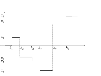
Figure 3: The step function $\Phi_{\mathbf{h},\mathbf{x}}$.

Toward this end, let $\mathcal{S}$ be the set of all pairs of finite sequences

$$(\mathbf{h},\mathbf{x})\qquad\mbox{where }\mathbf{h}:=(h_{1},\ldots,h_{N}),\mathbf{x}:=(x_{1},\ldots,x_{N})$$

for some $N\geq 1$, with the properties

$$0<h_{1}<h_{2}<\cdots<h_{N},\qquad x_{1},x_{2},\ldots,x_{N}\in{\mathbb{R}}\setminus\{0\},$$

and whenever $i<j$ and $x_{i}$, $x_{j}$ have the same sign, then $|x_{i}|\leq|x_{j}|$.

For notational convenience, we will also use the indices $0,N+1,\infty$, and set

$$x_{0}:=0,\qquad x_{\infty}:=-x_{1}\quad\mbox{and}\quad h_{0}:=0,\qquad h_{N+1}:=h_{\infty}:=2h_{N}.$$

The mesh of the partition of $[0,h_{N}]$ induced by $\mathbf{h}$ is the number

$$\operatorname{mesh}(\mathbf{h}):=\min\{h_{i}-h_{i-1}\dvtx 1\leq i\leq N\}.$$

For a pair $(\mathbf{h},\mathbf{x})$ as above, we let $\mathcal{I}:=\{1,\ldots,N\}$ and $\mathcal{I}_{\infty}\subset\mathcal{I}$ the largest set of consecutive integers in $\mathcal{I}$ containing $N$ and for which all $x_{i}$ for $i\in\mathcal{I}_{\infty}$ have the same sign.

For an index $i\in\mathcal{I}$, let $i^{-}$ denote the greatest index $j\in\mathcal{I}$ less than $i$ so that $x_{i}$ and $x_{j}$ have the same sign, and let $i^{-}=0$ if there is no such index. Similarly, let $i^{+}$ denote the least index $j\in\mathcal{I}$ greater than $i$ so that $x_{i}$ and $x_{j}$ have the same sign, and let $i^{+}=\infty$ if there is no such index. In particular, $N^{+}=\infty$. Also let $\alpha,\beta$ denote the first index $i$ with positive and negative $x_{i}$, respectively, again with the value $\infty$ if there is no such index.

Consider the function $\Phi_{\mathbf{h},\mathbf{x}}$ with domain $[0,\infty)$ and value $x_{0}=0$ on the interval $[0,h_{1}]$, $x_{i}$ on the interval $(h_{i},h_{i+1}]$ for $i\in\{1,\ldots,N-1\}$ and $x_{N}$ on $(h_{N},\infty)$; see Figure 3. Recall the definition of the graph occupation measure $m(\cdot)$ from the Introduction, and let

$$\mu_{\mathbf{h},\mathbf{x}}:=m(\Phi_{\mathbf{h},\mathbf{x}}).$$

We will use the shorthand notation $I(\mathbf{h},\mathbf{x})$ for the rate corresponding to this measure, namely

$$I(\mathbf{h},\mathbf{x}):=I(\mu_{\mathbf{h},\mathbf{x}})=\frac{\pi^{2}}{2}\sum_{i\in\mathcal{I}\setminus\mathcal{I}_{\infty}}\frac{|x_{i}-x_{i^{-}}|}{h_{i}^{2}}+\frac{\pi^{2}}{8}\sum_{i\in\mathcal{I}_{\infty}}\frac{|x_{i}-x_{i^{-}}|}{h_{i}^{2}}.$$ (3)

3 Confining Brownian motion—the upper bound

The goal of this section is to prove the core of the large deviations upper bound of Section 5.

In what follows, $m$ denotes the graph occupation measure, $B$ a standard two-sided Brownian motion and $x$ the process-of-wells mapping.

Proposition 5 ((Large deviation upper bound))

For each $\mu\in\mathcal{M}$ and $A<I(\mu)$, there exists an open neighborhood ${\mathcal{U}}$ of $\mu$ so that for all sufficiently large $M$, we have

$$\mathbf{P}\bigl{(}m(x_{B}/M)\in{\mathcal{U}}\bigr{)}\leq e^{-AM}.$$

The proof of this proposition is given in Lemmas 6 and 7. We first define neighborhoods that will be easy to handle. Using the notation of Section 2, for $(\mathbf{h},\mathbf{x})\in\mathcal{S}$ and $\varepsilon>0$, we define the following open set of measures:

$${\mathcal{U}}(\mathbf{h},\mathbf{x},\varepsilon)$$

(4)

$$\quad:=\left\{\nu\in\mathcal{M}\dvtx\begin{array}[]{l@{ \qquad}l}\nu\bigl{(}(h_{i}-\varepsilon,h_{i}+\varepsilon)\times(x_{i},\infty)\bigr{)}>0&\mbox{for $i\in\mathcal{I}$, }x_{i}>0\\ \nu\bigl{(}(h_{i}-\varepsilon,h_{i}+\varepsilon)\times(-\infty,x_{i})\bigr{)}>0&\mbox{for $i\in\mathcal{I}$, }x_{i}<0\end{array}\right\}.$$

We claim that these neighborhoods cover everything efficiently, even for small $\varepsilon$.

Lemma 6

For each $\mu\in\mathcal{M}$ and $A<I(\mu)$, there exists $(\mathbf{h},\mathbf{x})\in\mathcal{S}$ so that $I(\mathbf{h},\mathbf{x})>A$ and ${\mathcal{U}}(\mathbf{h},\mathbf{x},\varepsilon)\ni\mu$ for all $\varepsilon>0$.

The proof of this topological lemma is standard, but a bit technical. We postpone it to Section 9.

Lemma 7

For $(\mathbf{h},\mathbf{x})\in\mathcal{S}$, $A<I(\mathbf{h},\mathbf{x})$ and all small enough $\varepsilon>0$, there is an integer $M_{\varepsilon}$ so that

$$\mathbf{P}\bigl{(}m(x_{B}/M)\in{\mathcal{U}}(\mathbf{h},\mathbf{x},\varepsilon)\bigr{)}\leq e^{-AM}\qquad\mbox{for all }M\geq M_{\varepsilon}.$$ (7)

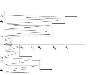
Figure 4: The restrictions on the reflected process.

For a two-sided Brownian motion $B$, we define its reflection from its past minimum as the process

$$R(t):=B(t)-\inf\{B(s)\dvtx s\mbox{ between 0 and }t\}$$ (8)

for all $t\in\mathbb{R}$. This process appears naturally in the study of the wells created by $B$.

Proof of Lemma 7 For a locally bounded function $Q\dvtx\mathbb{R}\to\mathbb{R}$, define

$$\underline{Q}(t) := \inf\{Q(s)\dvtx s\mbox{ between 0 and }t\},$$ (9)

$$\overline{Q}(t) := \sup\{Q(s)\dvtx s\mbox{ between 0 and }t\}$$ (10)

for all $t\in\mathbb{R}$.

Recall the mapping $\mu\mapsto(f_{\mu},g_{\mu})$ defined in the Introduction. For almost all Brownian paths $B$, the measure $\mu:=m(x_{B}/M)$ satisfies

$$Mf_{\mu}=f_{m(x_{B})}=\overline{x_{B}},\qquad Mg_{\mu}=g_{m(x_{B})}=\overline{(x_{B})^{-}}.$$

Also, $\mu\in{\mathcal{U}}(\mathbf{h},\mathbf{x},\varepsilon)$ implies $f_{\mu}(h_{i}+\varepsilon)>x_{i}$ for $x_{i}>0$, and similarly for $x_{i}<0$. Then, for $i\in\mathcal{I}$ with $x_{i}>0$, we have

$$\overline{x_{B}}(h_{i}+\varepsilon)>Mx_{i}\quad\Rightarrow\quad\overline{R}(Mx_{i})<h_{i}+\varepsilon,$$

because otherwise an ascent on the right with height at least $h_{i}+\varepsilon$ is created before $Mx_{i}$. This can be paired with an ascent on the negative axis of height at least $h_{i}+\varepsilon$, and the two will make $\overline{x_{B}}(h_{i}+\varepsilon)$ to be located in $(-\infty,Mx_{i}]$, a contradiction. This and the symmetric argument for negative $x_{i}$ shows that, on the event in the statement of the lemma, we have

$$\overline{R}(Mx_{i})<h_{i}+\varepsilon\qquad\mbox{for all }i\in\mathcal{I}.$$

For $M=1$, a realization of the process $R$ satisfying these restrictions is depicted in Figure 4.

There is one more piece of information we have for the path at the points $Mx_{i}$ for all indices $i\in\mathcal{I}\setminus\mathcal{I}_{\infty}$ when this set is nonempty. That is,

$$\underline{B}(Mx_{i})\geq-h_{N}-\varepsilon.$$

To see this, assume without loss of generality that $x_{i}>0$. Since $\mu\in{\mathcal{U}}(\mathbf{h},\mathbf{x},\varepsilon)$, we have

$$\mu\bigl{(}(h_{i}-\varepsilon,h_{i}+\varepsilon)\times(x_{i},\infty)\bigr{)}>0,$$

and thus $x_{B}(h^{\prime})>Mx_{i}>0$ for some $h^{\prime}\in(h_{i}-\varepsilon,h_{i}+\varepsilon)$. Let

$$h^{*}:=\inf\{h>h^{\prime}\dvtx x_{B}(h)<0\}.$$

We first argue that $h^{*}$ is well defined, that is, the above set is not empty. Since $i\in\mathcal{I}\setminus\mathcal{I}_{\infty}$, there is $j>i$ with $x_{j}<0$, and thus $x_{B}(h)<0$ for some $h\in(h_{j}-\varepsilon,h_{j}+\varepsilon)$. Since $\varepsilon<\operatorname{mesh}(\mathbf{h})/2$, we have $h_{j}-\varepsilon>h_{i}+\varepsilon$, and so indeed we have $h>h^{\prime}$. Also, $h^{*}<h_{N}+\varepsilon$.

At $h^{*}$, $x_{B}$ is positive because it is left continuous, but just after that it is negative. This means that the well of $x_{B}(h^{*})$ has depth exactly $h^{*}$. But $B(x_{B}(h^{*}))=\underline{B}(x_{B}(h^{*}))$, and combining this with $x_{B}(h^{*})\geq x_{B}(h^{\prime})>Mx_{i}$, we obtain

$$-h_{N}-\varepsilon<-h^{*}\leq\underline{B}(x_{B}(h^{*}))\leq\underline{B}(Mx_{i}).$$

Thus the event of the lemma is contained on the event

$$C_{M}:=\left\{\begin{array}[]{l@{ \qquad}l}\overline{R}(Mx_{i})<h_{i}+\varepsilon&\mbox{for }i\in\mathcal{I},\\ \underline{B}(Mx_{i})\geq-h_{N}-\varepsilon&\mbox{for }i\in\mathcal{I}\setminus\mathcal{I}_{\infty}\end{array}\right\}.$$

Recall from Section 2 that $i^{-}$ refers to the index preceding $i$ so that $x_{i}$ and $x_{i^{-}}$ have the same sign. Let $\mathbf{P}_{r,y}$ denote the law of the Markov process $(\overline{R},\underline{B})$ started at the point $(r,y)$. By the Markov property applied consecutively at $Mx_{i^{-}}$ for $i\in\mathcal{I}$, we get

$$\mathbf{P}(C_{M}) \leq \prod_{i\in\mathcal{I}\setminus\mathcal{I}_{\infty}}\sup_{r\geq 0,y\leq 0}\mathbf{P}_{r,y}\bigl{(}\overline{R}\bigl{(}M(x_{i}-x_{i^{-}})\bigr{)}<h_{i}+\varepsilon,$$

$$\hphantom{\prod_{i\in\mathcal{I}\setminus\mathcal{I}_{\infty}}\sup_{r\geq 0,y\leq 0}\mathbf{P}_{r,y}\bigl{(}}\underline{B}\bigl{(}M(x_{i}-x_{i^{-}})\bigr{)}\geq-h_{N}-\varepsilon\bigr{)}$$

$${}\times\prod_{i\in\mathcal{I}_{\infty}}\sup_{r\geq 0,y\leq 0}\mathbf{P}_{r,y}\bigl{(}\overline{R}\bigl{(}M(x_{i}-x_{i^{-}})\bigr{)}<h_{i}+\varepsilon\bigr{)}.$$

As usual, the product over an empty index set is 1. Note that the process $(\overline{R},-\underline{B})$ is nondecreasing in both coordinates of its starting point $(r,-y)$. Therefore we have the upper bound

$$\prod_{i\in\mathcal{I}\setminus\mathcal{I}_{\infty}}\mathbf{P}_{0,0}\bigl{(}\overline{R}\bigl{(}M(x_{i}-x_{i^{-}})\bigr{)}<h_{i},\underline{B}\bigl{(}M(x_{i}-x_{i^{-}})\bigr{)}\geq-h_{N}-\varepsilon\bigr{)}$$

$$\qquad{}\times\prod_{i\in\mathcal{I}_{\infty}}\mathbf{P}_{0,0}\bigl{(}\overline{R}\bigl{(}M(x_{i}-x_{i^{-}})\bigr{)}<h_{i}+\varepsilon\bigr{)}.$$

Then Lemma 20 implies that

$$\lim_{M\to\infty}\frac{\log\mathbf{P}(C_{M})}{M}\leq-I(\mathbf{h},\mathbf{x})-o(\varepsilon),$$

where $o(\varepsilon)$ depends on $(\mathbf{h},\mathbf{x})$ only. The claim follows.

4 Making a vessel—the lower bound

The goal of this section is to prove the large deviation lower bound. This can be formulated as follows:

Proposition 8 ((Large deviation lower bound))

For every open set $G\subset\mathcal{M}$, every $A>\inf_{G}I$ and for all sufficiently large $M$, we have

$$\mathbf{P}\bigl{(}m(x_{B}/M)\in G\bigr{)}\geq e^{-AM}.$$

Again, we proceed in two steps. We will first define a convenient set of Brownian paths, $\mathcal{R}(\mathbf{h},\mathbf{x},\varepsilon,\delta)$, and then prove a topological lemma that reduces the problem to showing that these paths have high probability.

Lemma 9

For every open $G\subset\mathcal{M}$, and every $A>\inf_{G}I$, there exists $(\mathbf{h},\mathbf{x})\in\mathcal{S}$ so that $I(\mathbf{h},\mathbf{x})<A$ and

$$\{m(x_{B})\dvtx B\in\mathcal{R}(\mathbf{h},\mathbf{x},\varepsilon,\varepsilon)\}\subset G$$

for all small enough $\varepsilon>0$.

The proof of this topological lemma is postponed to Section 9. In light of this lemma, it suffices to give a lower bound on the probability that for $B$ two-sided Brownian motion, $m(x_{B})$ is close to $\mu_{\mathbf{h},\mathbf{x}}$ in the large deviation regime. In fact, we will do this for a more restrictive set, namely for the event that $x_{B}$ is close in the Skorokhod topology to $\Phi_{\mathbf{h},\mathbf{x}}$.

Recall the Skorokhod topology on left continuous paths on $[0,\infty)$ with right limits. We call a set $A$ of these paths an $[a,b]$-Skorokhod neighborhood of $f$ if it is the inverse image of a Skorokhod neighborhood of $f|[a,b]$ under the restriction map.

Proposition 10

Let $(\mathbf{h},\mathbf{x})\in\mathcal{S}$. Then every $[0,2h_{N}]$-Skorokhod neighborhood of $\Phi_{\mathbf{h},\mathbf{x}}$ contains the image of the set $\mathcal{R}(\mathbf{h},\mathbf{x},\delta,\varepsilon)$ under the map $x$ for all $\delta,\varepsilon$ small enough, and Brownian motion $B$ satisfies

$$\lim_{M\to\infty}\frac{1}{M}\log\mathbf{P}\bigl{(}B(M\cdot)\in\mathcal{R}(\mathbf{h},\mathbf{x},\delta,\varepsilon)\bigr{)}=-I(\mathbf{h},\mathbf{x})+O_{\mathbf{h},\mathbf{x}}(\delta,\varepsilon).$$ (11)

The rest of this section contains the proof of the proposition. First, we construct the desired set of paths, then we show that they can be arbitrarily close to $\Phi_{\mathbf{h},\mathbf{x}}$, and finally we prove the desired probability decay.

Each path in $\mathcal{R}(\mathbf{h},\mathbf{x},\delta,\varepsilon)$ forms a “vessel,” in which when water is poured from the $y$ axis, the process of wells is close to $\Phi_{\mathbf{h},\mathbf{x}}$ almost until depth $2h_{N}$ is reached.

Construction

We define the following events, that is, sets of continuous functions $f\dvtx\mathbb{R}\to\mathbb{R}$, for $\varepsilon,\delta\in(0,1),h>0$ and $x,y\in{\mathbb{R}}$ with $0\leq x<y$ or $y<x\leq 0$. For all events, we require that, in the second endpoint of the interval mentioned, $f$ takes a value in $[0,h-\varepsilon h]$; this is to make the building blocks fit together well. In addition, we require:

1. between times $x(1+\delta),y(1-\delta)$, $f$ stays in $[-\varepsilon^{2}h,h]$.

2. between times $y(1-\delta),y$, $f$ stays in $[-\varepsilon h,h]$, visits below $-\varepsilon h+\varepsilon^{2}h$.

3. between times $y(1-\delta),y$, $f$ stays in $[0,h]$, visits $0$.

4. between times $y,y(1+\delta)$, $f$ stays in $[-\varepsilon^{2}h,h+\varepsilon h]$, visits above $h$.

We omit the dependence on $\varepsilon,\delta$ from the notation.

Our basic restriction set, $\mathcal{R}(\mathbf{h},\mathbf{x},\delta,\varepsilon)$, is defined as the intersection of the following sets $E_{i}$, for $i\in\mathcal{I}\cup\{0\}$. Our goal is to ensure that functions $f$ in these sets will have the property that $x_{f}$ is $[0,2h_{N}]$-Skorokhod-close to $\Phi_{\mathbf{h},\mathbf{x}}$. We will comment on the importance of the individual sets $E_{i}$ after their definition.

The beginning

$$E_{0} := C\bigl{(}0,x_{\alpha}\delta/(1-\delta),h_{\alpha}\bigr{)}\cap B(x_{\alpha}\delta,h_{\alpha})$$

$${}\cap C\bigl{(}0,x_{\beta}\delta/(1-\delta),h_{\beta}\bigr{)}\cap B(x_{\beta}\delta,h_{\beta}).$$

For $f\in E_{0}$, we have

$$x_{f}(h)\in\bigl{(}\delta(1+\delta)x_{\beta},\delta(1+\delta)x_{\alpha}\bigr{)}\qquad\mbox{for }h\in[0,h_{1}],$$

because the two barrier sets create a well around zero of depth at least $h_{1}$.

The indices in $\mathcal{I}\setminus\mathcal{I}_{\infty}$

For each index $i\in\mathcal{I}\setminus\mathcal{I}_{\infty}$, we define the set

$$E_{i}:=C(w_{i},x_{i},h_{i})\cap H(x_{i},h_{i})\cap B(x_{i},h_{i^{+}}),$$

where for all $i\in\mathcal{I}$, we let

$$w_{i}:=\cases{\displaystyle x_{i^{-}},&\quad$i\neq\alpha,\beta$,\cr\displaystyle x_{i}\delta,&\quad$i=\alpha$ or $\beta$.}$$

The purpose of $E_{i}$ is to guarantee that for $f\in E_{0}\cap\cdots\cap E_{i}$, the value of $x_{f}(\cdot)$ will be near $x_{i}$ for a time interval very close to $[h_{i},h_{i+1}]$.

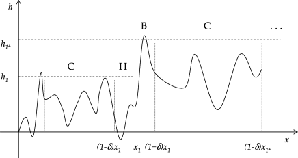
Figure 5: The first positive blocks of the construction.

More precisely, assume that $x_{i}>0$, and focus on the positive half of the path $f|[0,\infty)$. See Figure 5 for the case $i=1$. What $E_{i}$ adds to the intersection is that $f|[0,\infty)$ up to the point $x_{i}(1-\delta)$ does not reach a new minimum or maximum. Then it creates a new minimum (hole) near $x_{i}$, and then a barrier of height $h_{i^{+}}$ ahead of it. But $E_{i^{-}}$ has already created a barrier of height about $h_{i}$. Moreover, on the negative side there is a barrier of height at least $h_{i+1}$ following a minimum for $f|(-\infty,0]$ which is not deeper than the hole in the event $E_{i}$. So indeed, the value of $x_{f}(\cdot)$ will be near $x_{i}$ at least for a time interval almost equal to $[h_{i},h_{i+1}]$.

Note also that the barrier created by $E_{i}$ makes sure that from height about $h_{i}$ until height about $h_{i^{+}}$, the process $x_{f}$ either stays constant or jumps to negative values; that is, it does not advance to another positive value.

The indices in $\mathcal{I}_{\infty}$

By symmetry, we may assume that the $x_{i}$’s for $i\in\mathcal{I}_{\infty}$ are positive. For a locally bounded function $f$ defined in $\mathbb{R}$, and $z$ fixed, let $R_{z}f\dvtx[z,\infty)\to[0,\infty)$ denote $f$ reflected from its running minimum after $z$, namely

$$R_{z}f(x):=f(x)-\inf_{s\in[z,x]}f(s).$$ (13)

Let $q=\min\mathcal{I}_{\infty}$. For $i\in\mathcal{I}_{\infty}$, define the set $E_{i}$ of paths $f$ so that $R_{w_{q}(1+\delta)}f$ is in

$$C(w_{i},x_{i},h_{i})\cap H^{R}(x_{i},h_{i})\cap B(x_{i},h_{i^{+}}),$$

and $f$ satisfies

$$f(x)-f\bigl{(}w_{i}(1+\delta)\bigr{)}\leq\varepsilon^{2}\qquad\mbox{for }x\in[w_{i}(1+\delta),x_{i}(1+\delta)].$$ (14)

Note that $i^{+}=i+1$ unless $i=N$.

In order to understand these events $E_{i}$, we first consider the effect of the preceding events $E_{0}\cap\cdots\cap E_{q-1}$. See Figure 6.

Assume first that $\mathcal{I}_{\infty}\not=\mathcal{I}$. In this case, $E_{0}\cap\cdots\cap E_{q-1}$ puts restriction on the path on the interval $[x_{q-1}(1+\delta),w_{q}(1+\delta)]$. The minimum value of $f$ there is negative of order $\varepsilon$, the maximum is attained in the interval $[x_{q-1}(1+\delta),x_{q-1}]$, where the path goes over $2h_{N}$ because $(q-1)^{+}=\infty$ and $h_{\infty}=2h_{N}$.

When $\mathcal{I}_{\infty}=\mathcal{I}$, the event $E_{0}$ puts restriction on the path on the interval $[-x_{1}\delta(1+\delta),w_{q}(1+\delta)]$. The minimum value of $f$ there is negative of order $\varepsilon$, the maximum is attained on $[-x_{1}\delta(1+\delta),-x_{1}\delta]$, where the path goes over $2h_{N}$.

In both cases, the maximum on $[0,w_{q}(1+\delta)]$ is attained in the interval $[w_{q},w_{q}(1+\delta)]$, where the path goes a bit over $h_{q}$ and ends up in $[0,h_{q}-\varepsilon h_{q}]$.

Figure 6: The last part.

Then the set $E_{q}$ requires from $f$ up to the point $x_{q}(1-\delta)$ not to create an ascent of height larger than $h_{q}$ (see Figure 6) and then to create one with lowest point having $x$-coordinate in $(x_{q}(1-\delta),x_{q}(1+\delta))$ and height around $h_{q^{+}}$. The goal of (14) is to force $f$ not to go above $h_{q}$, and this is obtained because as we noted $f(w_{q}(1+\delta))\leq h_{q}-\varepsilon h_{q}$, and from that point on $f$ stays below $h_{q}-\varepsilon h_{q}+\varepsilon^{2}$. These, together with the barrier of height $2h_{N}$ on the negative axis, guarantee that $x_{f}(h)$ is around $x_{q}$ at least for $h$ in an interval very close to $[h_{q},h_{q^{+}}]$.

The other $E_{i}$’s with $i\in\mathcal{I}_{\infty}$ work in the same way.

The behavior of $x_{f}$ for $f\in\mathcal{R}(\mathbf{h},\mathbf{x},\delta,\varepsilon)$

We will now examine more precisely how $x_{f}$ behaves when $f\in\mathcal{R}(\mathbf{h},\mathbf{x},\delta,\varepsilon)$. For $x,y\in\mathbb{R}$, define

$$f^{\#}(x,y)=\cases{\displaystyle\sup\{f(t)-f(s)\dvtx x\leq s\leq t\leq y\},&\quad$x\leq y$,\cr\displaystyle\sup\{f(t)-f(s)\dvtx y\leq t\leq s\leq x\},&\quad$x\geq y$.}$$

Also let

$$\tilde{h}_{1}:=\max\{f(x)\dvtx x\mbox{ between 0 and }x_{1}\delta(1+\delta)\},$$

and let $z_{1}$ be the closest to zero point between $0$ and $x_{\alpha\vee\beta}\delta(1+\delta)$ where $f$ takes the value $\tilde{h}_{1}$. In the interval between $z_{1}$ and $x_{1}\delta(1+\delta)$, we have a well of depth around $h_{1}$. Its exact depth is

$$v_{1}:=\tilde{h}_{1}-\min\{f(x)\dvtx x\mbox{ between $z_{1}$ and }x_{1}\delta(1+\delta)\}.$$

Also define

$$v_{i}:=\cases{\displaystyle f^{\#}\bigl{(}x_{i-1},x_{i}\delta(1+\delta)\bigr{)},&\quad if $i=\alpha\vee\beta\neq\infty$,\cr\displaystyle f^{\#}\bigl{(}x_{i-1}(1-\delta),x_{i-1}(1+\delta)\bigr{)},&\quad if $i-1=i^{-}\in\mathcal{I}\setminus\mathcal{I}_{\infty}$,\cr\displaystyle f^{\#}\bigl{(}x_{i-1},x_{i^{-}}(1+\delta)\bigr{)},&\quad if $i-1\neq i^{-}\in\mathcal{I}\setminus\mathcal{I}_{\infty}$.}$$

Now for $i^{-}\in\mathcal{I}_{\infty}$ let

$$v_{i}:=\sup\bigl{\{}R_{w_{q}(1+\delta)}f(x)\dvtx x\in[x_{i^{-}},x_{i^{-}}(1+\delta)]\bigr{\}},$$

and finally let $v_{N+1}=2h_{N}$. From the above discussion and the definition of $\mathcal{R}(\mathbf{h},\mathbf{x},\delta,\varepsilon)$, we conclude that

$$v_{i}\in\cases{\displaystyle[h_{1},h_{1}+\varepsilon(h_{1}+\varepsilon h_{\alpha\vee\beta})],&\quad if $i=1$,\cr\displaystyle[h_{i}+(\varepsilon-\varepsilon^{2})h_{i-1},h_{i}+\varepsilon(h_{i}+h_{i-1})],&\quad if $i=\alpha\vee\beta\neq\infty$\cr&\qquad or $i^{-}\in\mathcal{I}\setminus\mathcal{I}_{\infty}$,\cr\displaystyle(h_{i},h_{i}+\varepsilon h_{i}],&\quad if $i^{-}\in\mathcal{I}_{\infty}$,}$$ (15)

and

$$\displaystyle|x_{f}(h)|\leq\delta(\delta+1)(x_{\alpha}\vee|x_{\beta}|)\qquad\mbox{for }h\in[0,v_{1}],$$

(16)

$$\displaystyle x_{f}(h)\mbox{ is between }x_{i}(1-\delta),x_{i}\qquad\mbox{for }h\in(v_{i},v_{i+1}],i\in\mathcal{I}.$$

We assumed that $\varepsilon$ is small enough so that $v_{1}<v_{2}<\cdots<v_{N}$, and $-\varepsilon h_{i}+\varepsilon^{2}h_{i}<-\varepsilon h_{i-1}$ for $i\in\mathcal{I}\setminus\mathcal{I}_{\infty}$. Informally, the second requirement guarantees that, for these $i$’s, the set $H(x_{i},h_{i})$ creates a new, deeper minimum, and this is used for (4).

Relations (15), (4) show that any $[0,2h_{N}]$-Skorokhod neighborhood of $\Phi_{\mathbf{h},\mathbf{x}}$ contains $\{x_{f}\dvtx f\in\mathcal{R}(\mathbf{h},\mathbf{x},\delta,\varepsilon)\}$ if $\varepsilon$, $\delta$ are small enough.

The asymptotic probability of $\mathcal{R}(\mathbf{h},\mathbf{x},\delta,\varepsilon)$

It remains to prove (11).

We apply the Markov property and use Lemma 21. Note that for any two restriction sets concerning contiguous intervals, say $[x,y],[y,z]$, with $0<x<y<z$, the allowed values for $f(y-)$ are the same as the ones on which we condition in the first three relations of Lemma 21. If the second set corresponds to an index in $\mathcal{I}_{\infty}$, the ending point of the first block is irrelevant.

It is also important that the limits computed in that lemma are uniform over the starting points of the processes involved. These observations allow us to conclude that the left-hand side of (11) equals

$$-\frac{\pi^{2}}{2}\sum_{i=\alpha,\beta}\frac{|x_{i}|\delta}{h_{i}^{2}}\biggl{(}\frac{1}{(1+\varepsilon^{2})^{2}}+\frac{\delta}{(1+\varepsilon+\varepsilon^{2})^{2}}\biggr{)}$$

$$\qquad{}-\frac{\pi^{2}}{2}\sum_{i\in\mathcal{I}\setminus\mathcal{I}_{\infty}}\biggl{(}\frac{|x_{i}-w_{i}-\delta(x_{i}+w_{i})|}{h_{i}^{2}(1+\varepsilon^{2})^{2}}+\frac{\delta|x_{i}|}{h_{i}^{2}(1+\varepsilon)^{2}}+\frac{\delta|x_{i}|}{h_{i^{+}}^{2}(1+\varepsilon+\varepsilon^{2})^{2}}\biggr{)}$$

$$\qquad{}-\frac{\pi^{2}}{8}\sum_{i\in\mathcal{I}_{\infty}}\biggl{(}\frac{|x_{i}-w_{i}-\delta w_{i}|}{h_{i}^{2}}+\frac{\delta|x_{i}|}{h_{i^{+}}^{2}(1+\varepsilon)^{2}}\biggr{)},$$

which is $-I(\mathbf{h},\mathbf{x})+O_{\mathbf{h},\mathbf{x}}(\delta,\varepsilon)$. Note that for $\delta\searrow 0$, only the confinement sets appearing in $E_{i}$, for $i\in\mathcal{I}$, contribute to the rate of decay. The reason is that all other sets put restrictions on intervals of size proportional to $\delta$. Similarly, the first restriction set $E_{0}$ does not contribute.

5 The large deviation principle for the process of wells

In this section, we complete the proof of the large deviation principle for the family $\{m(x_{B}/M)\dvtx M>0\}$ stated in Theorem 2.

Recall that a family $\{\mu_{M}\dvtx M>0\}$ of Borel measures on a topological space $\mathcal{M}$ satisfies the large deviation principle with rate $I\dvtx\mathcal{M}\to[0,\infty]$ as $M\to\infty$ if for every measurable set $\mathcal{B}\subset\mathcal{M}$ and every $A>\inf_{\mathcal{B}^{\circ}}I$ and $A^{\prime}<\inf_{\bar{\mathcal{B}}}I$ we have

$$-A\leq\frac{\log\mu_{M}(\mathcal{B})}{M}\leq-A^{\prime}$$ (17)

for all sufficiently large $M$, where ${\mathcal{B}}^{\circ},\bar{\mathcal{B}}$ denote the interior and the closure of $\mathcal{B}$, respectively.

Recall also that $I$ is a good rate function if $I^{-1}[0,A]$ is compact for all finite $A$. In particular, these sets are closed, which is equivalent to $I$ being lower semicontinuous.

We have established in Propositions 5, 8 the core upper and lower bounds. Next, we prove exponential tightness. Recall that a family of measures $\{\mu_{M}\dvtx M>0\}$ as above is exponentially tight as $M\to\infty$ if for every $A>0$ there is a compact set $\mathcal{Q}\subset\mathcal{M}$ so that $\mu_{M}(\mathcal{Q}^{c})<e^{-AM}$ for all large enough $M$.

Lemma 11

The family $\{m(x_{B}/M)\dvtx M>0\}$ is exponentially tight.

By the definition of $\mathcal{M}$, for every $a>0$, the set

$$\mathcal{Q}_{a}:=\Biggl{\{}\mu\in\mathcal{M}\dvtx\operatorname{supp}(\mu)\subset\bigcup_{k=1}^{\infty}[k-1,k]\times[-ak^{3},ak^{3}]\Biggr{\}}$$ (18)

is compact in $\mathcal{M}$. Recall definitions (8) and (10). We have

$$\mathbf{P}\bigl{(}m(x_{B}/M)\in\mathcal{Q}_{a}^{c}\bigr{)} \leq \sum_{k=1}^{\infty}\mathbf{P}\bigl{(}\max\{\overline{x_{B}}(k),\overline{(x_{B})^{-}}(k)\}\geq aMk^{3}\bigr{)}$$

$$\leq 2\sum_{k=1}^{\infty}\mathbf{P}\bigl{(}\overline{x_{B}}(1)\geq aMk\bigr{)}$$

using the scaling and symmetry properties of $x_{B}$. But for all $x>0$, we have that $\overline{x_{B}}(1)\geq x$ implies $\bar{R}(x)<1$, which has probability at most

$$\mathbf{P}\bigl{(}B[0,x]\subset(-1,1)\bigr{)}\leq Ce^{-x\pi^{2}/8}$$

with $C$ a constant. Here we used the fact that $R$ has the same law as $|B|$ and relation (38). Consequently,

$$\mathbf{P}\bigl{(}m(x_{B}/M)\in\mathcal{Q}_{a}^{c}\bigr{)}\leq C^{\prime}e^{-Ma\pi^{2}/8}$$ (20)

for a constant $C^{\prime}$. Since $a$ was arbitrary, exponential tightness follows.

Proof of Theorem 2, the large deviation principle The first inequality in (17) is a reformulation of Proposition 8 applied to the open set $\mathcal{B}^{\circ}$. For the second, let $A<\inf_{\bar{\mathcal{B}}}I$. By exponential tightness (Lemma 11) there exists a compact set $\mathcal{Q}$ so that

$$P\bigl{(}m(x_{B}/M)\in\mathcal{Q}^{c}\bigr{)}\leq e^{-AM}$$

for all sufficiently large $M$. Each point in $\mathcal{Q}\cap\bar{\mathcal{B}}$ can be covered with an open set satisfying the same asymptotic bound by Proposition 5. To get the second inequality of (17), take a finite subcover of the compact set $\mathcal{Q}\cap\bar{\mathcal{B}}$, and use the union bound.

Finally, we show that $I$ is a good rate function. Take $A>0$ and $\mu\in I^{-1}(A,\infty]$. By Proposition 5, $\mu$ has an open neighborhood $\mathcal{U}$ so that

$$-A>\limsup_{M\to\infty}\frac{\log P(m(x_{B}/M)\in\mathcal{U})}{M}.$$

The right-hand side is bounded below by $-\inf_{\mathcal{U}}I$ because of the large deviation lower bound. Thus $\mathcal{U}\subset I^{-1}(A,\infty]$, which shows that the latter set must be open. Thus $I^{-1}[0,A]$ is closed. On the other hand, exponential tightness and the large deviation lower bound gives $\inf_{\mathcal{Q}^{c}}I>A$ for some compact $\mathcal{Q}$, so $I^{-1}[0,A]\subset\mathcal{Q}$ must also be compact.

6 The limit points of the environment

For $a>1$, and $B\dvtx\mathbb{R}\to\mathbb{R}$ a continuous path, we define the function $Z_{a}\dvtx[0,\infty)\to\mathbb{R}$ by

$$Z_{a}(s):=\frac{x_{B}(sa)}{a^{2}\log\log a}$$ (21)

for all $s\geq 0$. We will determine the limit points of the family of measures $(m(Z_{a}))_{a>e}$, as $a\to\infty$, with respect to the topology of local weak convergence, when $B$ is a two-sided Brownian path. Then Theorem 1 will follow from localization results connecting $x_{B}$ with the Sinai walk. We start by doing this along geometric sequences.

Geometric sequences

In the next proposition, we show that all limit points of $(m(Z_{a}))_{a>e}$ along geometric sequences fall into a certain set $\mathcal{K}$. Then Proposition 13 shows that in fact along any geometric sequence, all points of $\mathcal{K}$ are limit points.

Proposition 12

If $c>1$, then with probability one, every subsequence of $\{m(Z_{c^{n}})\dvtx n>1/\log c\}$ has a further convergent subsequence, and the limit points of the original sequence are contained in the set

$$\mathcal{K}:=\{\mu\in\mathcal{M}\dvtx I(\mu)\leq 1\}.$$

By the scaling property of $x_{B}$ and (20),

$$\mathbf{P}\bigl{(}m(Z_{c^{n}})\in\mathcal{Q}_{a}^{c}\bigr{)}=\mathbf{P}\bigl{(}m(x_{B}/\log\log c^{n})\in\mathcal{Q}_{a}^{c}\bigr{)}\leq C^{\prime}\exp\biggl{(}-\frac{a\pi^{2}}{8}\log\log c^{n}\biggr{)}.$$

For $a>8/\pi^{2}$, the first Borel–Cantelli lemma implies that $m(Z_{c^{n}})\in\mathcal{Q}_{a}$ eventually, and the first claim follows by the compactness of $\mathcal{Q}_{a}$.

For each point in $\mathcal{K}^{c}$, Proposition 5 provides an open set $\mathcal{U}$ containing it so that for some $A(\mathcal{U})>1$ and for all large enough $n$, we have

$$\mathbf{P}\bigl{(}m(Z_{c^{n}})\in\mathcal{U}\bigr{)}\leq\exp\bigl{(}-A(\mathcal{U})\log\log c^{n}\bigr{)}.$$ (22)

Now each such set $\mathcal{U}$ can be written as a union of elements of a fixed countable base. Thus $K^{c}$ can be covered with a countable collection of open sets $\mathcal{U}_{k}$ satisfying (22). By the first Borel–Cantelli Lemma and the union bound, no $\mathcal{U}_{k}$ contains a limit point a.s.

The promised complement of Proposition 12 is as follows.

Proposition 13

If $c>1$, then with probability one, the limit points of $\{m(Z_{c^{n}})\dvtx n>1/\log c\}$ include the points of the set

$$\mathcal{K}:=\{\mu\in\mathcal{M}\dvtx I(\mu)\leq 1\}.$$

Note that it suffices to prove that every open set $\mathcal{U}$ intersecting $\mathcal{K}$ contains a limit point with probability one. Using this claim for all such elements $\mathcal{U}$ of a countable base for $\mathcal{M}$, we conclude that the limit points are a.s. dense in $\mathcal{K}$. Since they form a closed set, this set must contain $\mathcal{K}$.

By Lemma 26 the minimum of $I$ on an open set is either $0$, $\infty$ or is not achieved. Therefore every open set $\mathcal{U}$ intersecting $\mathcal{K}$ has $\inf_{\mathcal{U}}I<1$. By Lemma 9, there exists $(\mathbf{h},\mathbf{x})\in\mathcal{S}$ so that $I(\mathbf{h},\mathbf{x})<1$ and

$$\{m(x_{B})\dvtx B\in\mathcal{R}(\mathbf{h},\mathbf{x},\varepsilon,\varepsilon)\}\subset\mathcal{U}$$

for all small enough $\varepsilon>0$.

Define $n_{0}=\lfloor 1/\log c\rfloor+2$, and for $n\geq n_{0}$, let $A_{n}$ be the set of paths $B$ so that the rescaling satisfies

$$\frac{B(c^{2n}\log\log c^{n}\times\cdot)}{c^{n}}\in\mathcal{R}(\mathbf{h},\mathbf{x},\varepsilon,\varepsilon).$$

Note that if a path $B$ belongs to $A_{n}$, then the corresponding path $Z_{c^{n}}$ from (21) satisfies $m(Z_{c^{n}})\in\mathcal{U}$. Thus it suffices to show that $A_{n}$ i.o. a.s.

Since

$$A_{n}=\mathcal{R}(\mathbf{h}c^{n},\mathbf{x}c^{2n}\log\log c^{n},\varepsilon,\varepsilon),$$ (23)

the scaling property of Brownian motion implies

$$\mathbf{P}(A_{n})=\mathbf{P}(\mathcal{R}(\mathbf{h},\mathbf{x}\log\log c^{n},\varepsilon,\varepsilon)).$$

Then Proposition 10 gives

$$\liminf_{n\to\infty}\frac{\log\mathbf{P}(A_{n})}{\log\log c^{n}}\geq-I(\mathbf{h},\mathbf{x})-O_{\mathbf{h},\mathbf{x}}(\varepsilon)>-(1-\delta_{1})$$

for some $\delta_{1}\in(0,1-I(\mathbf{h},\mathbf{x}))$ and all small enough $\varepsilon$. Consequently, there is an $n_{1}$ so that for $n\geq n_{1}$ we have $\mathbf{P}(A_{n})\geq n^{-1+\delta_{1}}$. Then for all $n$,

$$\sum_{k=n_{0}}^{n}\mathbf{P}(A_{k})>Cn^{\delta_{1}}$$ (24)

for an appropriate constant $C>0$. In particular, $\sum\mathbf{P}(A_{k})=\infty$. In order to conclude that $A_{n}$ i.o., we use a correlation bound given in the upcoming Lemma 14. Let $\Sigma_{n}:=1_{A_{n_{0}}}+\cdots+1_{A_{n}}$. We write

$$\mathbf{E}(\Sigma_{n}^{2})=\mathbf{E}\Sigma_{n}+2\mathop{\mathop{\sum}_{k=n_{0}}}_{l>k}^{n}\mathbf{P}(A_{k}\cap A_{l}).$$

Let $\Delta,C_{0}$ be as in Lemma 14, and $d_{k}:=\Delta+(\log\log k)/(2\log c)$. We bound the probabilities $\mathbf{P}(A_{k}\cap A_{l})$, $n_{0}\leq k<l\leq n$, in one of two ways, according whether $|k-\ell|\leq d_{k}$, thus getting for their sum the upper bound

$$C_{0}\mathop{\mathop{\sum}_{k=n_{0}}}_{l-k>d_{k}}^{n}\mathbf{P}(A_{k})\mathbf{P}(A_{l})+d_{n}\sum_{k=n_{0}}^{n}\mathbf{P}(A_{k})\leq\biggl{(}\frac{C_{0}}{2}+\frac{d_{n}}{\mathbf{E}(\Sigma_{n})}\biggr{)}(\mathbf{E}\Sigma_{n})^{2}.$$

But $d_{n}/\mathbf{E}(\Sigma_{n})\to 0$ by (24), so that the Kochen–Stone lemma [Durrett (2010), Exercise 2.3.20] gives

$$\mathbf{P}(A_{n}\mbox{ i.o.})\geq\limsup_{n\to\infty}\frac{(\mathbf{E}\Sigma_{n})^{2}}{\mathbf{E}(\Sigma_{n}^{2})}\geq 1/C_{0}.$$ (25)

To prove that $\{A_{n}\mbox{ i.o.}\}$ holds a.s., we will prove that it is a tail event, that is, that it belongs to the $\sigma$-algebra $\bigcap_{t>0}\sigma(B(s)\dvtx|s|\geq t)$, and we will apply Theorem 8.2.7 from Durrett (2010).

To see this, fix $t_{0}>0$. A function $f\dvtx\mathbb{R}\to\mathbb{R}$ belongs to $A_{n}$ if its values on a certain interval around zero satisfy certain conditions imposed by the sets whose intersection defines $A_{n}$. For $n$ that satisfies $t_{0}<\varepsilon(x_{\alpha}\wedge|x_{\beta}|)c^{2n}\log\log c^{n}$, we isolate the conditions concerning the values of $f$ on $[-t_{0},t_{0}]$ and write

$$A_{n} = \mathcal{R}(\mathbf{h}c^{n},\mathbf{x}c^{2n}\log\log c^{n},\varepsilon,\varepsilon)$$

$$= C\bigl{(}0,c^{2n}(\log\log c^{n})x_{\alpha}\varepsilon/(1-\varepsilon),c^{n}h_{\alpha}\bigr{)}$$

$${}\cap C\bigl{(}0,c^{2n}(\log\log c^{n})x_{\beta}\varepsilon/(1-\varepsilon),c^{n}h_{\beta}\bigr{)}\cap C_{n}$$

$$= C\bigl{(}0,t_{0}/(1-\varepsilon),c^{n}h_{\alpha}\bigr{)}\cap C\bigl{(}t_{0}/(1+\varepsilon),c^{2n}(\log\log c^{n})x_{\alpha}\varepsilon/(1-\varepsilon),c^{n}h_{\alpha}\bigr{)}$$

$${}\cap C\bigl{(}0,-t_{0}/(1-\varepsilon),c^{n}h_{\beta}\bigr{)}$$

$${}\cap C\bigl{(}-t_{0}/(1+\varepsilon),c^{2n}(\log\log c^{n})x_{\beta}\varepsilon/(1-\varepsilon),c^{n}h_{\beta}\bigr{)}\cap C_{n}$$

$$= C\bigl{(}0,t_{0}/(1-\varepsilon),c^{n}h_{\alpha}\bigr{)}\cap C\bigl{(}0,-t_{0}/(1-\varepsilon),c^{n}h_{\beta}\bigr{)}\cap A_{n}^{\prime},$$

where $C_{n}$ is the intersection of the remaining sets involved in the definition of $A_{n}$, and

$$A_{n}^{\prime} := C\bigl{(}t_{0}/(1+\varepsilon),c^{2n}(\log\log c^{n})x_{\alpha}\varepsilon/(1-\varepsilon),c^{n}h_{\alpha}\bigr{)}$$

$${}\cap C\bigl{(}-t_{0}/(1+\varepsilon),c^{2n}(\log\log c^{n})x_{\beta}\varepsilon/(1-\varepsilon),c^{n}h_{\beta}\bigr{)}\cap C_{n}.$$

Now $\{A_{n}\mbox{ i.o.}\}\subset\{A_{n}^{\prime}\mbox{ i.o.}\}$, but also $\{A_{n}^{\prime}\mbox{ i.o.}\}\subset\{A_{n}\mbox{ i.o.}\}$ since every function $f$ in the first set belongs to $C(0,t_{0}/(1-\varepsilon),c^{n}h_{\alpha})\cap C(0,-t_{0}/(1-\varepsilon),c^{n}h_{\beta})$ provided that $\max\{|f(s)|\dvtx|s|\leq t_{0}\}<\varepsilon^{2}(h_{\alpha}\vee h_{\beta})c^{n}$. And the last inequality holds for all large $n$ because $c>1$, and $f$ is bounded on $[-t_{0},t_{0}]$, being continuous. Since for all large $n$ we have $A_{n}^{\prime}\in\sigma(B(s)\dvtx|s|\geq t_{0})$, it follows that $\{A_{n}\mbox{ i.o.}\}\in\sigma(B(s)\dvtx|s|\geq t_{0})$, and this proves our assertion.

The next lemma shows a version of near independence for the family of sets $\{A_{n}\dvtx n\geq 1\}$, defined in the proof of Proposition 13, and uses the notation set up in that proof.

Lemma 14

There are $\Delta,C_{0}\in(0,\infty)$ depending on $\mathbf{h},\mathbf{x},\varepsilon$ such that

$$\mathbf{P}(A_{k}\cap A_{l})\leq C_{0}\mathbf{P}(A_{k})\mathbf{P}(A_{l})$$

for $k\geq n_{0}$ and

$$l-k>\Delta+\frac{1}{2}\frac{\log\log k}{\log c}.$$ (26)

For the pair $(\mathbf{h},\mathbf{x})\in\mathcal{S}$, we will use the notation of Section 2.

We assume that $x_{N}>0$. Let $p$ equal $\max(\mathcal{I}\setminus\mathcal{I}_{\infty})$ if the set is nonempty, and $\infty$ otherwise. For any integer $n\geq n_{0}$, define

$$J_{n}:=c^{2n}\log\log c^{n}[x_{p}(1+\varepsilon),x_{N}(1+\varepsilon)].$$

Recall that $x_{\infty}=-x_{1}$. $J_{n}$ is the interval where $A_{n}$ imposes restrictions on $B$.

$A_{l}$ is the intersection of several requirements the first of which [the two confinement sets of $E_{0}$ in (4)] refers to the time interval

$$F_{l}:=c^{2l}\log\log c^{l}[\varepsilon x_{\beta},\varepsilon x_{\alpha}].$$

We would like to have $l$ so large that $J_{k}$ will be in the interior of $F_{l}$, so that knowing that $A_{k}$ happened does not influence much the probability of $A_{l}$. We ensure that $J_{k}\subset F_{l}/2$ by assuming that

$$l>k+\frac{1}{2\log c}\biggl{\{}\log\biggl{(}\frac{|x_{p}|}{|x_{\beta}|}\vee\frac{x_{N}}{x_{\alpha}}\biggr{)}+\log\frac{2(1+\varepsilon)}{\varepsilon}\biggr{\}}$$ (27)

for the rest of the proof. Note that (27) is implied by (26) with an appropriate choice of $\Delta$. We let

$$A^{+}=\{B|[0,\infty)\dvtx B\in A\},\qquad A^{-}=\{B|(-\infty,0]\dvtx B\in A\}.$$

It is enough to prove the claim of the lemma for the pairs $\{A^{+}_{k},A^{+}_{l}\},\{A_{k}^{-},A_{l}^{-}\}$ as they are independent. We will do it for the first. Let

$$\Theta_{l}:=h_{\alpha}c^{l}[-\varepsilon^{2},1]\supset h_{\alpha}c^{l}\biggl{[}-\frac{\varepsilon^{2}}{2},1-\frac{\varepsilon^{2}}{2}\biggr{]}=:\tilde{\Theta}_{l}$$

and

$$A^{+}_{k,l}:=A^{+}_{k}\cap\{B(s)\in\Theta_{l}\mbox{ for }0<s\in J_{k}\}.$$

Paths $B$ in $A_{l}$ satisfy $B(F_{l}\cap[0,\infty))\subset\Theta_{l}$. So that $A^{+}_{k}\cap A^{+}_{l}=A^{+}_{k,l}\cap A^{+}_{l}$ since $J_{k}\subset F_{l}$. Let $A^{+}_{l}(J_{k})$ denote the paths that satisfy the restrictions put by $A^{+}_{l}$ for the time interval $J_{k}$, and define $A^{+}_{l}(J_{l}\setminus J_{k})$ analogously. Denote by $j_{k}$ the right endpoint of $J_{k}$, and let

$$q(x):=\mathbf{P}\bigl{(}A^{+}_{l}(J_{l}\setminus J_{k})|B_{j_{k}}=x\bigr{)}.$$

We have

$$A^{+}_{k}\cap A^{+}_{l}=A^{+}_{k,l}\cap A^{+}_{l}\subset A^{+}_{k,l}\cap A^{+}_{l}(J_{l}\setminus J_{k}),$$

and the probability of the right-hand side can be written as

$$\mathbf{E}[{\mathbf{1}}_{A^{+}_{k,l}}q(B_{j_{k}})]\leq\mathbf{P}(A^{+}_{k})\max_{\Theta_{l}}q.$$

On the other hand,

$$\mathbf{P}(A^{+}_{l}) = \mathbf{P}\bigl{(}A^{+}_{l}(J_{l}\setminus J_{k})\cap A^{+}_{l}(J_{k})\bigr{)}=\mathbf{E}\bigl{[}{\mathbf{1}}_{A^{+}_{l}(J_{k})}q(B_{j_{k}})\bigr{]}$$

$$\geq \mathbf{P}\bigl{(}A^{+}_{l}(J_{k})\mbox{ and }B_{j_{k}}\in\tilde{\Theta}_{l}\bigr{)}\min_{\tilde{\Theta}_{l}}q.$$

So that

$$\frac{\mathbf{P}(A^{+}_{k}\cap A^{+}_{l})}{\mathbf{P}(A^{+}_{k})\mathbf{P}(A^{+}_{l})}\leq\frac{\max_{\Theta_{l}}q}{\min_{\tilde{\Theta}_{l}}q}\mathbf{P}\bigl{(}A^{+}_{l}(J_{k})\mbox{ and }B_{j_{k}}\in\tilde{\Theta}_{l}\bigr{)}^{-1}.$$ (28)

To bound the last term, note that $B|[0,\infty)\in A^{+}_{l}(J_{k})$ follows from $B([0,j_{k}])\subset\tilde{\Theta}_{\ell}$. The restriction (26) on $l-k$ shows that

$$c^{2k-2l}\log\log c^{k}<c^{-2\Delta}\biggl{(}1+\frac{\log\log c}{\log 2}\biggr{)}=:c_{1}.$$

This and Brownian scaling yield the lower bound

$$\mathbf{P}\bigl{(}A^{+}_{l}(J_{k})\mbox{ and }B_{j_{k}}\in\tilde{\Theta}_{l}\bigr{)}\geq\mathbf{P}\biggl{(}B\bigl{(}[0,c_{1}(1+\varepsilon)x_{N}]\bigr{)}\subset h_{\alpha}\biggl{[}-\frac{\varepsilon^{2}}{2},1-\frac{\varepsilon^{2}}{2}\biggr{]}\biggr{)},$$

which is positive and does not depend on $k,l$.

To bound the fraction in the right-hand side of (28), note that with $f_{l}$ the right endpoint of $F_{l}$, the event $A^{+}_{l}(F_{l}\setminus J_{k})$ is equivalent to $B([j_{k},f_{l}])\subset\Theta_{\ell}$ and $B_{f_{l}}\in[0,(1-\varepsilon)h_{\alpha}c^{l}]$, by the definition of the confinement set $C(0,x_{\alpha}\varepsilon/\break(1-\varepsilon),h_{\alpha})$. Let $r(x,y)$ denote the density of $B(f_{l})$ for Brownian motion started from $x$ at time $j_{k}$ restricted to this event. By the Markov property, we have

$$q(x)=\int r(x,y)\mathbf{P}\bigl{(}A^{+}_{l}(J_{l}\setminus F_{l})|B(f_{l})=y\bigr{)}\,dy,$$

which gives the bound

$$\frac{\max_{\Theta_{l}}q}{\min_{\tilde{\Theta}_{l}}q}\leq\max\biggl{\{}\frac{r(x_{1},y)}{r(x_{2},y)}\dvtx x_{1}\in\Theta_{l},x_{2}\in\tilde{\Theta}_{l},y\in[0,(1-\varepsilon)h_{\alpha}c^{l}]\biggr{\}}.$$

With the notation introduced in the beginning of Section 8, we have

$$r(x,y)=Q^{(1+\varepsilon^{2})h_{\alpha}c^{l}}(f_{l}-j_{k},x+\varepsilon^{2}h_{\alpha}c^{l},y+\varepsilon^{2}h_{\alpha}c^{l}),$$

and (38), (39) give that the above maximum is bounded above by a constant (that depends only on $\varepsilon$) as long as

$$\frac{f_{l}-j_{k}}{(1+\varepsilon^{2})^{2}h_{\alpha}^{2}c^{2l}}\geq t_{0}(\varepsilon).$$

This holds for $k,l$ satisfying (26) provided that $\Delta$ is large enough.

From geometric sequences to the full family

We will now show that Propositions 12, 13 imply the result for the full family. As noted in Vervaat (1990), this can be done easily using the scaling properties of the rate function $I$ and the regular variation of the scaling factor $a^{2}\log\log a$ in (21).

Proposition 15

With probability one, every sequence $(m(Z_{t_{k}}))_{k\geq 1}$ with $t_{k}\to\infty$ has a convergent subsequence, and the set of all possible limit points is exactly

$$\mathcal{K}:=\{\mu\in\mathcal{M}\dvtx I(\mu)\leq 1\}.$$

For a measure $\mu\in\mathcal{M}$ and $a>0$, let $\mu_{a}\in\mathcal{M}$ denote the rescaled version of $\mu$ defined on every product of measurable sets $H\times X\subset[0,\infty)\times\mathbb{R}$ as

$$\mu_{a}(H\times X)=a\mu(a^{-1}H\times a^{-2}X).$$

Then for all continuous functions $\psi\dvtx[0,\infty)\times\mathbb{R}\to\mathbb{R}$ with compact support,

$$\int\psi(h,x)\,d\mu_{a}(h,x)=a\int\psi(ah,a^{2}x)\,d\mu(h,x).$$ (29)

Also, $f_{\mu_{a}}(t)=a^{2}f_{\mu}(t/a)$ for all $t\geq 0$, and the analogous statement holds for $g_{\mu_{a}}$. Consequently, $I(\mu_{a})=I(\mu)$.

For $t>1$, let $\mu^{(t)}=m(Z_{t})$. We will use the following claim.

If $\mu\!\in\!\mathcal{M}$, and for two sequences $(t_{k})_{k\geq 1},(p_{k})_{k\geq 1}$ with $\lim_{k\to\infty}t_{k}\!=\infty,\lim_{k\to\infty}t_{k}/p_{k}=a\in(0,\infty)$ we have $\mu^{(p_{k})}\to\mu$, then $\mu^{(t_{k})}\to\mu_{1/a}$.

Take $\psi\dvtx[0,\infty)\times\mathbb{R}\to\mathbb{R}$ continuous of compact support. For $k\geq 1$, we may assume that $p_{k},t_{k}\geq 1$, and let

$$a_{k}:=\frac{t_{k}}{p_{k}},\qquad\beta_{k}:=\frac{\log\log p_{k}}{\log\log t_{k}}.$$

Then $\int\psi(h,x)\,d\mu^{(t_{k})}(h,x)$ equals

$$\int_{0}^{\infty}\psi\biggl{(}t,\frac{x_{B}(a_{k}p_{k}t)}{a_{k}^{2}p_{k}^{2}\log\log t_{k}}\biggr{)}\,dt = a_{k}^{-1}\int_{0}^{\infty}\psi\biggl{(}a_{k}^{-1}s,a_{k}^{-2}\beta_{k}\frac{x_{B}(p_{k}s)}{p_{k}^{2}\log\log p_{k}}\biggr{)}\,ds$$

$$= a_{k}^{-1}\int\psi(a_{k}^{-1}h,a_{k}^{-2}\beta_{k}x)\,d\mu^{(p_{k})}(h,x)$$

$$= aa_{k}^{-1}\int\psi(aa_{k}^{-1}h,a^{2}a_{k}^{-2}\beta_{k}x)\,d\mu^{(p_{k})}_{1/a}(h,x).$$

The last equality follows form (29). Since $aa_{k}^{-1}\to 1$ and $\mu^{(p_{k})}_{1/a}\to\mu_{1/a}$, it suffices to prove that

$$\int\psi(aa_{k}^{-1}h,a^{2}a_{k}^{-2}\beta_{k}x)\,d\mu^{(p_{k})}_{1/a}(h,x)-\int\psi(h,x)\,d\mu^{(p_{k})}_{1/a}(h,x)\to 0$$

as $k\to\infty$.

Let $C$ be the set of points in $[0,\infty)\times\mathbb{R}$ with Euclidean distance at most 1 from the support of $\psi$, and $h^{*}$ the maximum of the first projection of $C$. For $\varepsilon>0$, using the compactness of $C$, the uniform continuity of $\psi$, and the fact that $\mu^{(p_{k})}_{1/a}\in\mathcal{M}$, we obtain that for large $k$, the absolute value of the last difference is bounded from above by

$$\int_{C}\varepsilon d\mu^{(p_{k})}_{1/a}(h,x)\leq\varepsilon h^{*}.$$

This proves the claim.

Now let $t_{k}\to\infty$ be a sequence. We fix a $c>1$, and write this sequence uniquely as $t_{k}=a_{k}c^{i_{k}}$ with integers $i_{k}$ and real numbers $a_{k}\in[1,c)$.

Regarding the first assertion of the proposition, note that by Proposition 12, $m(Z_{c^{i_{k}}})$ has limit points in $\mathcal{K}$. Pick one, say $\mu$, and then passing to a further subsequence along which $a_{k}$ converges to some limit $a(c)\in[1,c]$, we see using the claim above that $\mu_{1/a(c)}$ is a limit point along the sequence $t_{k}$.

For the second assertion, we have by Propositions 12, 13 that almost surely, all limit points along $c^{k}$ are exactly the elements of the set $\mathcal{K}$. It remains to show that along the above sequence $(t_{k})_{k\geq 1}$, we do not get limit points outside $\mathcal{K}$. If $\mu^{\prime}$ is a limit point along $t_{k}$, then as above, we pass to a further subsequence along which $a_{k}$ converges to some limit $a(c)\in[1,c]$. It follows again from the claim above that along $c^{i_{k}}$, $\mu^{\prime}_{a(c)}$ is a limit point. By Proposition 12, we have $I(\mu^{\prime}_{a(c)})\leq 1$. So that $I(\mu^{\prime})=I(\mu^{\prime}_{a(c)})\leq 1$, that is, $\mu^{\prime}\in\mathcal{K}$.

7 The limit points of the motion

The continuous time and space analogue of Sinai’s walk is diffusion in random environment, that is, the diffusion $X$ with $X(0)=0$ that satisfies the formal differential equation

$$dX(t)=d\beta(t)-\tfrac{1}{2}V^{\prime}(X(t))\,dt.$$ (30)

Here, $\beta$ is standard Brownian motion, and $V$, the environment, is a random function we pick before running the diffusion. For the rigorous definition of this diffusion, as well as its relation with Sinai’s walk; see Shi (2001), Seignourel (2000).

In this work, we will consider diffusions run in a Brownian-like environment. That is, we require from the measure governing $V$ to be such that there is, on a possibly enlarged probability space, a standard two-sided Brownian motion $B$ such that for all $n\geq 1$, we have

$$\mathbf{P}\Bigl{(}\sup_{|x|\leq n}|V(x)-B(x)|\geq C_{1}\log n\Bigr{)}\leq\frac{1}{n^{C_{2}}}$$ (31)

for some constants $C_{1},C_{2}$. For these environments, the diffusion does not explode in finite time. Moreover, its behavior is dominated by the environment, and one aspect of this phenomenon is captured by the following result. Recall the definition of $x_{B}$ from Section 2.

Theorem 16 ([Hu (2000), Theorem 1.1])

Assume that $V$ satisfies (31). For every $\delta_{1}>0$, there exists $C,t_{0}>0$ so that for $t\geq t_{0}$ and $\lambda\geq 1$, we have

$$\mathbf{P}\bigl{(}|X(t)-x_{B}(\log t)|>\lambda\bigr{)}\leq C\biggl{(}\frac{\log\log t}{\sqrt{\lambda}}+\frac{1}{(\log t)^{1-\delta_{1}}}\biggr{)}.$$ (32)

The limit points of the diffusion

For the diffusion defined by (30), where $V$ satisfies (31), we have the following analog of Theorem 1.

Theorem 17

With probability 1, the limit points, as $a\to\infty$, in the topology of local weak convergence of the graph occupation measures of the random functions

$$y_{a}:=\frac{X(e^{at})}{a^{2}\log\log a},\qquad t\geq 0,$$

constitute the set

$$\mathcal{K}:=\{\mu\in\mathcal{M}\dvtx I(\mu)\leq 1\}.$$

Also, there is at least one limit point along every sequence $a_{n}\to\infty$.

Note that if $f_{n},g_{n}$ is a sequence of functions on $[a,b]$ with $m(f_{n})\to\mu$ and $f_{n}-g_{n}\to 0$ in (Lebesgue) measure, then $m(g_{n})\to\mu$. Indeed, assuming that for bounded, uniformly continuous $\varphi$ we have

$$\int_{a}^{b}\varphi(t,f_{n}(t))\,dt\to\int_{[a,b]\times{\mathbb{R}}}\varphi\,d\mu,$$

we break down the integral to the set where $|f_{n}(s)-g_{n}(s)|<\varepsilon$ and its complement. Since $\varphi$ is uniformly continuous, on this set the integrand is close to $\varphi(t,g_{n}(t))$, while the measure of the complement of this set is small. Thus $m(g_{n})\to\mu$.

Using this observation, Proposition 15 and the definition of the topology of $\mathcal{M}$, it is clear that to prove Theorem 17, it suffices to show that for every $0<\varepsilon<M<\infty$, as $a\to\infty$ we have

$$\mathcal{L}\{s\in[\varepsilon,M]\dvtx|X(e^{as})-x_{B}(as)|>\varepsilon a^{2}\log\log a\}\to 0.$$

We prove this for $0<\varepsilon<M=1$, as this is in no way different than the general $M$ case. By changing variables $w=as$, the above quantity will become

$$\int_{a\varepsilon}^{a}\frac{{\mathbf{1}}(|X(e^{w})-x_{B}(w)|>\varepsilon a^{2}\log\log a)}{a}\,dw$$

$$\qquad\leq\int_{a\varepsilon}^{\infty}\frac{{\mathbf{1}}(|X(e^{w})-x_{B}(w)|>\varepsilon w^{2}\log\log w)}{w}\,dw.$$

If the last integral is finite for some $a>0$, then it converges to $0$ as $a\to\infty$. Its expectation is bounded using Theorem 16, provided $a$ satisfies $\varepsilon a>\log t_{0}$ and $(\varepsilon a)^{2}\log\log(\varepsilon a)>1$, by

$$\int_{a\varepsilon}^{\infty}\frac{1}{w}\mathbf{P}\bigl{(}|X(e^{w})-x_{B}(w)|>\varepsilon w^{2}\log\log w\bigr{)}\,dw$$

$$\qquad\leq\int_{a\varepsilon}^{\infty}\frac{c}{w}\biggl{(}\frac{\log w}{\sqrt{w^{2}\log\log w}}+\frac{1}{w^{1-\delta_{1}}}\biggr{)}\,dw<\infty.$$

So that the integral is finite with probability 1.

The limit points of the walk

To prove Theorem 1, we will embed the walk it in a diffusion generated by an appropriate random environment $V$.

Let $(S_{n})_{n\geq 1}$ be Sinai’s walk with $\operatorname{Var}(\log((1-p_{1})/p_{1}))=1$. Define the step potential $V$ as follows: $V(0)=0$, and for every $n\in{\mathbb{Z}}$, $V$ is constant in $[n-1,n)$, and jumps at $n$ by $V(n)-V(n-)=\log((1-p_{n})/p_{n})$. This potential can be placed on a possibly enlarged probability space with a two-sided Brownian motion $B$ so that (31) is satisfied. This follows from the strong approximation theorem of Komlós–Major–Tusnády [Theorem 1 in Komlós, Major and Tusnády (1976)]. The theorem requires that $Y:=\log((1-p_{1})/p_{1})$ has $\mathbf{E}(e^{\lambda Y})<\infty$ for $\lambda$ in a neighborhood of 0, which is exactly the assumption we made for the law of $p$ in the Introduction.

The walk can be embedded in the diffusion $X$ run in the environment $V$ as follows. Let $t_{0}=0$ and $t_{n}=\inf\{t>t_{n-1}\dvtx|X(t)-X(t_{n-1})|=1\}$ for $n\geq 1$.

Theorem 18 ([Hu and Shi (1998), Proposition 9.1])

$(X(t_{n}))_{n\geq 1}$ has the same law as $(S_{n})_{n\geq 1}$. Moreover, $\{t_{n+1}-t_{n}\dvtx n\geq 1\}$ are i.i.d. with distribution that of the first hitting time $T$ of 1 for reflected standard Brownian motion.

We will need the fact that the law of $1/T$ has exponential tails. This holds since if $1/T>x>0$, then the maximum or the negative of the minimum of Brownian motion on $[0,1/x]$ is at least 1. Since the maximum has the same distribution as $|B(x)|$, we have

$$P(1/T>x)\leq 2P\bigl{(}|B(1/x)|>1\bigr{)}=4P\bigl{(}B(1)>\sqrt{x}\bigr{)}\leq ce^{-x/2}.$$ (33)

Proof of Theorem 1 Let $t(\cdot)$ be the the piecewise linear continuous extension of $t_{n}$ so that $t(n)=t_{n}$. To prove the theorem, it suffices to show that for every $0<\varepsilon<M<\infty$, as $a\to\infty$,

$$\frac{S(e^{as})-x_{B}(as)}{a^{2}\log\log a}\to 0\qquad\mbox{in measure on $[\varepsilon,M]$, a.s.}$$

Since $|S(s)-X(t(s))|\leq 1$, it suffices to show the previous claim with $X(t(e^{as}))$ instead of $S(e^{as})$. We break this down into two parts, namely

$$\frac{X(t(e^{as}))-x_{B}(\log t(e^{as}))}{a^{2}\log\log a}\to 0,\qquad\frac{x_{B}(as)-x_{B}(\log t(e^{as}))}{a^{2}\log\log a}\to 0$$ (34)

in measure on the interval $[\varepsilon,M]$ as $a\to\infty$. We assume for simplicity that $M=1$. Proceeding the same way as for the diffusion, for the first claim it suffices to prove that

$$\int_{\varepsilon a}^{\infty}\frac{1}{w}{\mathbf{1}}\bigl{(}|X(t(e^{w}))-x_{B}(\log t(e^{w}))|>\varepsilon w^{2}\log\log w\bigr{)}\,dw<\infty$$

for some $a>0$. The function $t$ has derivative equal to $t_{n}-t_{n-1}$ in $(n-1,n)$, and undefined in $n$ for every positive integer $n$. The integral over the $w$’s with $1/t^{\prime}(e^{w})>\log w$ has expectation bounded above by

$$\mathbf{E}\int_{\varepsilon a}^{\infty}\frac{1}{w}{\mathbf{1}}\bigl{(}1/t^{\prime}(e^{w})>\log w\bigr{)}\,dw=\int_{\varepsilon a}^{\infty}\frac{1}{w}\mathbf{P}\bigl{(}1/t^{\prime}(e^{w})>\log w\bigr{)}\,dw,$$

which is finite because $1/t^{\prime}$ has the same distribution as $1/T$ in (33). For the rest of the integral, we change variables $r=\log t(e^{w})$ and reduce the problem to the finiteness of

$$\int_{a\varepsilon}^{\infty}\frac{1}{w}\frac{t(e^{w})}{e^{w}}\frac{{\mathbf{1}}(1/t^{\prime}(e^{w})\leq\log w)}{t^{\prime}(e^{w})}{\mathbf{1}}\bigl{(}|X(e^{r})-x_{B}(r)|>\varepsilon w^{2}\log\log w\bigr{)}\,dr.$$

By the law of large numbers and the fact that $\mathbf{E}T=1$, we have $t(s)/s\to 1$. So $t(e^{w})/e^{w}\to 1$ as $r\to\infty$, which shows that $w/r\to 1$ as well. Thus the above integral is finite if

$$\int_{a\varepsilon}^{\infty}\frac{\log r}{r}{\mathbf{1}}\bigl{(}|X(e^{r})-x_{B}(r)|>(\varepsilon/2)r^{2}\log\log r\bigr{)}\,dr$$

is finite. This follows by taking expectations and using Theorem 16.

For the second convergence claim in (34), it suffices to show that

$$\int_{2}^{\infty}\frac{1}{w}{\mathbf{1}}\bigl{(}x_{B}(w)\not=x_{B}(\log t(e^{w}))\bigr{)}\,dw<\infty.$$

Note that $x_{B}(w)\not=x_{B}(\log t(e^{w}))$ implies that $x_{B}$ has a jump between $w$ and $\log t(e^{w})$. By the law of large numbers, for all $w$ large, this interval is contained in $(w-1,w+1)$. So it suffices to show the finiteness of the integral

$$\int_{2}^{\infty}\frac{1}{w}{\mathbf{1}}\bigl{(}x_{B}\mbox{ has a jump in }(w-1,w+1)\bigr{)}\,dw.$$

Applying Lemma 19, we bound its expectation from above by

$$c\int_{2}^{\infty}\frac{1}{w}\log\frac{w+1}{w-1}\,dw<\infty.$$

In the proof of Theorem 1, we use the next lemma, which gives a bound on the probability that $x_{B}$ jumps on an interval.

Lemma 19

The process $x_{B}$ satisfies $\mathbf{P}(x_{B}(s)\not=x_{B}(t))\leq c|\log(t/s)|$ for some finite constant $c$ and all $t,s>0$.

This holds because the jumps of $x_{B}(e^{t})$ form a translation-invariant point process on $\mathbb{R}$ with finite mean density $c$. Rather than proving this, we will invoke the exact formula for the above probability. Assuming that $s<t$, and using the scaling property of $x_{B}$ [see (2)], the probability in question equals $\mathbf{P}(x_{B}(1)\not=x_{B}(t/s))$. However,

$$\mathbf{P}\bigl{(}x_{B}(1)=x_{B}(t/s)\bigr{)}=\biggl{(}\frac{t}{s}\biggr{)}^{-2}\frac{5-2e^{-(t/s)+1}}{3}$$

as is shown in the proof of Theorem 2.5.13 in Zeitouni (2004). And this gives easily the required bound.

Proof of Corollary 3 In fact, we will prove that if $\gamma\dvtx[0,1]\to[0,\infty)$ is differentiable with $(t\mapsto t^{3}\gamma(t))$ nondecreasing, then

$$\limsup_{a\to\infty}\frac{1}{a^{2}\log\log a}\int_{0}^{1}\gamma(t)S(e^{at})\,dt=\frac{4}{\pi^{2}}s_{0}^{3}a(s_{0}),$$ (35)

where $s_{0}$ is any root of $2\int_{s}^{1}\gamma=s\gamma(s)$ in $(0,1)$.

For $H\dvtx[0,\infty)\times\mathbb{R}\to\mathbb{R}$ with compact support and whose projection of the set of the discontinuity points in the $x$-axis has Lebesgue measure zero, the map $(\mathcal{M}\ni\mu\mapsto\int H\,d\mu)$ is continuous in the weak topology, because any $\mu\in\mathcal{M}$ has first projection Lebesgue measure. Combining this with the definition of the graph occupation measure, we get

$$\limsup_{a\to\infty}\int_{0}^{\infty}H\biggl{(}t,\frac{S(e^{at})}{a^{2}\log\log a}\biggr{)}\,dt$$

(36)

$$\qquad=\sup\biggl{\{}\int H(x,y)\,d\mu(x,y)\dvtx\mu\in\mathcal{M},I(\mu)\leq 1\biggr{\}}.$$

Everywhere below, we use the abbreviation $A:=8/\pi^{2}$.

For the choice $H(x,y):=\gamma(x)y\mathbf{1}_{x\in[0,1],|y|\leq A+1}$ the limits in equations (35), (7) agree because by Theorem 1.3 in Hu and Shi (1998), it holds

$$\operatorname{\overline{\lim}}\limits_{n\to\infty}\frac{\max_{1\leq k\leq n}|S_{k}|}{(\log n)^{2}\log\log\log n}=A.$$

It remains to evaluate the supremum in (7) for this choice of $H$. If $\gamma$ is identically zero, the corollary holds trivially. So we assume that $\gamma$ is positive somewhere in $[0,1]$. Since $\gamma$ is nonnegative, it follows from the form of the rate function $I$ that the above supremum equals

$$\sup\biggl{\{}\int_{0}^{1}\gamma(t)f(t)\,dt\dvtx f(0)=0,f\mbox{ nondecreasing},\int_{0}^{1}t^{-2}\,df(t)\leq A\biggr{\}}.$$

We did not include the factor $\mathbf{1}_{|f(t)|\leq A+1}$ inside the integral because the conditions on $f$ imply that $0\leq f(t)=\int_{0}^{t}df(s)\leq\int_{0}^{1}s^{-2}\,df(s)\leq A$.

For a given nondecreasing $f\geq 0$, define $F(t):=\int_{0}^{t}s^{-2}\,df(s)$, so that $f(t)=\int_{0}^{t}s^{2}\,dF(s)$. We use this representation of $f$ and apply first Fubini’s theorem and then integration by parts in $\int_{0}^{1}\gamma(t)f(t)\,dt$ to write it as

$$\int_{0}^{1}F(s)r^{\prime}(s)\,ds,$$

where $r(s):=-s^{2}\int_{s}^{1}\gamma(t)\,dt$. Using the fact that $(t\mapsto t^{3}\gamma(t))$ is nondecreasing in $[0,1]$, we find that $r^{\prime}$ is nonpositive before $s_{0}$ and nonnegative after $s_{0}$. And since $F\leq A$, the above integral is bounded above by

$$-Ar(s_{0})=\frac{A}{2}s_{0}^{3}\gamma(s_{0}).$$

The last equality follows from $r^{\prime}(s_{0})=0$.

For the choice $f^{\gamma}(t)=s_{0}^{2}A\mathbf{1}_{(s_{0},\infty)}$, we get $\int_{0}^{1}\gamma(t)f^{\gamma}(t)\,dt=As_{0}^{2}\int_{s_{0}}^{1}\gamma(t)\,dt=As_{0}^{3}\gamma(s_{0})/2$, so that the supremum is achieved. Clearly, the only measure that achieves the supremum is the element of $\mathcal{M}$ that puts all its mass on the graph of $f^{\gamma}$.

Finally, for the case of the corollary, $\gamma(t)=t^{r}$, we compute $s_{0}=\eta_{r}:=(\frac{2}{r+3})^{1/(r+1)}$, while the value of the supremum is $(A/2)\eta_{r}^{r+3}$.

8 The probability of confinement

In this section, we compute the asymptotic decay of the probabilities that Brownian motion or Brownian motion reflected from its running minimum stay on certain bounded sets for large intervals of time.

Fix $h>0,x\in(0,h),t>0$, and let $Q^{h}(t,x,\cdot)$ be the density of the measure

$$S\mapsto\mathbf{P}_{x}\bigl{(}B_{t}\in S,B[0,t]\subset(0,h)\bigr{)}.$$

Proposition 8.2 in Port and Stone (1978) gives

$$Q^{1}(t,x,y)=2\sum_{n=1}^{\infty}e^{-n^{2}\pi^{2}t/2}\sin(n\pi x)\sin(n\pi y).$$ (37)

Using this and Brownian scaling, we get that there exists a universal constant $c_{2}$ so that for all $t\geq 1$, $x,y\in[0,h]$, we have

$$Q^{h}(t,x,y)\leq c_{2}h^{-1}\exp\biggl{(}-\frac{\pi^{2}}{2}\frac{t}{h^{2}}\biggr{)}.$$ (38)

Moreover, for every $\varepsilon>0$ there exists a constant $c_{1}=c_{1}(\varepsilon)$ so that for all $t\geq 1$, and $x,y\in[\varepsilon h,(1-\varepsilon)h]$, we have

$$Q^{h}(t,x,y)\geq c_{1}(\varepsilon)h^{-1}\exp\biggl{(}-\frac{\pi^{2}}{2}\frac{t}{h^{2}}\biggr{)}.$$ (39)

Recall from (9) the notation for the past minimum of a given process, and from (8) the process $R=B-\underline{B}$. The probability that $R$ stays confined in an interval for a large time interval $[0,t]$ decays exponentially in $t$. In the next lemma, we compute the exact rate of decay.

Lemma 20

For $K>0$, $\varepsilon\in[0,1/2)$, $w\in[0,1)$ and $z\in(0,1)$,

$$(\mathrm{a}) \lim_{t\to\infty}\frac{1}{t}\log\mathbf{P}_{z}\bigl{(}B([0,t])\subset[0,1],B(t)\in[\varepsilon,1-\varepsilon]\bigr{)}=-\frac{\pi^{2}}{2},$$

$$(\mathrm{b}) \lim_{t\to\infty}\frac{1}{t}\log\mathbf{P}\bigl{(}R([0,t])\subset[0,1],R(t)\in[0,1-\varepsilon]|R(0)=w\bigr{)}=-\frac{\pi^{2}}{8},$$

$$(\mathrm{c}) \lim_{t\to\infty}\frac{1}{t}\log\mathbf{P}_{0}\bigl{(}R([0,t])\subset[0,1],\underline{B}(t)\geq-K\bigr{)}=-\frac{\pi^{2}}{2}.$$

For $\varepsilon_{1}\in(0,1/2)$ fixed, the convergence in (a) is uniform over $z\in[\varepsilon_{1},1-\varepsilon_{1}]$, and the convergence in (b) is uniform over $w\in[0,1-\varepsilon_{1}]$.

Comparing (b) and (c), note the drastic effect of the restriction $\underline{B}(t)\geq-K$. The process $(R,-\underline{B})$ has the same law as $(|B|,L)$ where $L$ is the process of local time at zero for the Brownian motion $B$. Phrased in terms of $(|B|,L)$, the first event requires $B([0,t])\subset[-1,1]$, the other requires additionally that $L_{t}^{0}\leq K$, that is, $B$ does not hit zero many times. This restriction makes the second event more like $B([0,t])\subset(0,1]$, that is, $B$ is essentially restricted to an interval of half size than before.

(a) Follows by integrating (38) and (39) over $y$.

(b) Since $R$ has the same law as the absolute value of Brownian motion, the claim follows by the scaling property of Brownian motion and (a).

(c) Lower bound: Pick an open interval $V$ of length 1 around 0 that does not contain $-K$. Then

$$B([0,t])\subset V\quad\mbox{implies}\quad R([0,t])\subset[0,1],\qquad\underline{B}_{t}\geq-K.$$

By (a) applied with $\varepsilon=0$, the probability of the first event decays like $\exp(-t[\pi^{2}/\allowbreak 2+o(1)])$ as $t\to\infty$.

(c) Upper bound: Let $A_{t}$ denote the event in question. Subdivide the rectangle $[0,t]\times[-K,0]$ into $n\times n$ small isomorphic rectangles. Each rectangle is a product of a time interval ${\mathcal{T}_{i}}:=[(i-1)t/n,it/n]$ with $i=1,2,\ldots,n$ and a space interval. Consider the graph of the process $\underline{B}$, and let $J$ be the union of the subdivision rectangles it intersects. Fix $m\geq 1$. When $\underline{B}(t)\geq-K$, we have:

• $J=\bigcup_{i=1}^{n}{\mathcal{T}_{i}}\times{\mathcal{B}_{i}}$ for some space intervals $\mathcal{B}_{i}$.

• Let $\mathcal{N}=\{i\dvtx\mbox{length }\mathcal{B}_{i}\leq(m+2)K/n\}$. Then $|\mathcal{N}|\geq(1-1/m)n$.

The first claim is clear. For the second, note that on the time intervals $\mathcal{T}_{i}$ for $i\notin\mathcal{N}$ the process $\underline{B}$ decreases by at least $mK/n$. But the total decrease is at most $K$, so there are at most $n/m$ such indices $i$. We have

$$P(A_{t}) = P\bigl{(}\underline{B}(t)\geq-K,\mbox{ graph }B[0,t]\subset\mbox{graph }\underline{B}[0,t]+\{0\}\times[0,1]\bigr{)}$$

$$\leq \sum_{J}\mathbf{P}(\mbox{graph }B[0,t]\subset J+\{0\}\times[0,1]).$$

Here the sum is over all unions $J$ of rectangles satisfying the conditions above. By the Markov property, we get the upper bound

$$\sum_{J}\prod_{i=1}^{n}\max_{x}\mathbf{P}_{x}\bigl{(}B({\mathcal{T}_{i}})\subset{\mathcal{B}_{i}}+[0,1]\bigr{)}$$

$$\qquad\leq 2^{(n^{2})}\max_{x}\bigl{(}\mathbf{P}_{x}\bigl{(}B[0,t/n]\subset[0,1+(m+2)K/n]\bigr{)}\bigr{)}^{|\mathcal{N}|}.$$

The inequality follows by considering only the indices $i\in\mathcal{N}$. Brownian scaling, part (a) with $\varepsilon=0$ and the fact $|\mathcal{N}|\geq n(1-1/m)$ gives

$$\limsup_{t\to\infty}\frac{1}{t}\log\mathbf{P}(A_{t})\leq-\frac{1}{n}\biggl{(}\frac{\pi^{2}}{2}\frac{1}{(1+(m+2)K/n)^{2}}\biggr{)}n(1-1/m).$$

Since this holds for $m,n$ arbitrary, we let $n=m^{2}\to\infty$ to get the desired upper bound.

Below, we will use the operator $R_{x}$ of reflection from the past infimum, defined in (13), and the notation $R=R_{0}B$ from (8).

For $0\leq w\leq x<y$ and $0<h_{1}<h_{2}$, call $\Gamma(w,x,y,h_{1},h_{2})$ the set

$$\{R_{w}f\in C(x,y,h_{1})\cap H^{R}(y,h_{1})\cap B(y,h_{2})\}$$

$$\qquad{}\cap\bigl{\{}f-f\bigl{(}x(1+\delta)\bigr{)}\leq\varepsilon^{2}\mbox{ on }[x(1+\delta),y(1+\delta)]\bigr{\}},$$

which is involved in the definition of $\mathcal{R}(\mathbf{h},\mathbf{x},\delta,\varepsilon)$. More precisely, the set $E_{i}$ corresponding to an index $i\in\mathcal{I}_{\infty}$, defined in Section 4, is exactly the set

$$\Gamma\bigl{(}w_{q}(1+\delta),w_{i},x_{i},h_{i},h_{i^{+}}\bigr{)}.$$

The following lemma computes for large $M$ the probability that the scaled Brownian motion $B(M\cdot)$ is in the special sets $C,H,B,\Gamma$, defined in Section 4 and above.

Lemma 21

Let $0\leq x<y,0<h_{1}<h_{2},h>0$, and small enough $\varepsilon,\delta>0$.

Uniformly on $z\in[0,h-\varepsilon h],z_{1}\in[0,h_{1}-\varepsilon h_{1}],z_{2}\in\mathbb{R}$, as $M\to\infty$ we have:

$$(\mathrm{a}) \frac{1}{M}\log\mathbf{P}\bigl{(}B(M\cdot)\in C(x,y,h)|B\bigl{(}Mx(1+\delta)\bigr{)}=z\bigr{)}\to-\frac{\pi^{2}}{2}\frac{y-x-\delta(x+y)}{h^{2}(1+\varepsilon^{2})^{2}};$$

$$(\mathrm{b}) \frac{1}{M}\log\mathbf{P}\bigl{(}B(M\cdot)\in H(y,h)|B\bigl{(}My(1-\delta)\bigr{)}=z\bigr{)}\to-\frac{\pi^{2}}{2}\frac{\delta y}{h^{2}(1+\varepsilon)^{2}};$$

$$(\mathrm{c}) \frac{1}{M}\log\mathbf{P}\bigl{(}B(M\cdot)\in B(y,h_{2})|B(My)=z_{1}\bigr{)}\to-\frac{\pi^{2}}{2}\frac{\delta y}{h_{2}^{2}(1+\varepsilon+\varepsilon^{2})^{2}};$$

$$(\mathrm{d}) \frac{1}{M}\log\mathbf{P}\biggl{(}B(M\cdot)\in\Gamma\bigg{|}\begin{array}[]{l}R\bigl{(}Mx(1+\delta)\bigr{)}=z_{1}\\ B\bigl{(}Mx(1+\delta)\bigr{)}=z_{2}\end{array}\biggr{)}$$

$$\qquad\to-\frac{\pi^{2}}{8}\biggl{(}\frac{y-x-\delta x}{h_{1}^{2}}+\frac{\delta y}{h_{2}^{2}(1+\varepsilon)^{2}}\biggr{)},$$

where $\Gamma:=\Gamma(w,x,y,h_{1},h_{2})$ and the events $C,H,B,\Gamma$ depend on $\varepsilon,\delta$.

(a) It follows from Lemma 20(a) and the scaling property of Brownian motion.

(b) The exponential rate of decay of the event in question is the same as the one of confinement on $[-\varepsilon h,h]$ between times $y(1-\delta),y$ and ending in $[0,(1-\varepsilon)h]$. Because the difference of the two events is contained on the event of confinement on the smaller interval $[-\varepsilon h+\varepsilon^{2}h,h]$, which decreases exponentially faster. Thus, the result follows again from Lemma 20(a).

(c) The same reasoning as in part (b) proves this claim too.

(d) We can assume that $w=0$. Then we let $\Gamma(x,y,h_{1},h_{2})=\Gamma(0,x,y,h_{1},h_{2})$, and $\Gamma^{\prime}(x,y,h_{1},h_{2})$ to be only the first set in the intersection defining $\Gamma(x,y,\allowbreak h_{1},h_{2})$; that is, we remove the restriction $f-f(x(1+\delta))\leq\varepsilon^{2}$ on $[x(1+\delta),\break y(1+\delta)]$. We first prove the claim with $\Gamma^{\prime}$ in place of $\Gamma$. To this aim, we observe that

$$\lim_{M\to\infty}\frac{1}{M}\log\mathbf{P}\bigl{(}R(M\cdot)\in C(x,y,h_{1})|R\bigl{(}Mx(1+\delta)\bigr{)}=z_{1}\bigr{)}$$

(41)

$$\qquad=-\frac{\pi^{2}}{8}\frac{y-x-\delta(x+y)}{h_{1}^{2}},$$

$$\lim_{M\to\infty}\frac{1}{M}\log\mathbf{P}\bigl{(}R(M\cdot)\in H^{R}(y,h_{1})|R\bigl{(}My(1-\delta)\bigr{)}=z_{1}\bigr{)}=-\frac{\pi^{2}}{8}\frac{\delta y}{h_{1}^{2}},$$ (42)

$$\lim_{M\to\infty}\frac{1}{M}\log\mathbf{P}\bigl{(}R(M\cdot)\in B(y,h_{2})|R(My)=z_{1}\bigr{)}=-\frac{\pi^{2}}{8}\frac{\delta y}{h_{2}^{2}(1+\varepsilon)^{2}},$$ (43)

where the convergence is uniform over $z_{1}\in[0,h_{1}-\varepsilon h_{1}]$.

The first expression follows from Lemma 20(b). For the second, an upper bound is given by the same relation because the event requires confinement on $[0,h_{1}]$ for the time interval $[My(1-\delta),My\delta]$. For a lower bound, we will consider two events whose intersection is inside the event of interest and whose probability we will estimate. The first event

$$\left\{\begin{array}[]{c}\mbox{In the time interval }[My(1-\delta),My(1-\delta)+1],\\ \mbox{$R$ \mbox{ visits } 0, stays in $[0,h_{1}]$, ends in }[0,h_{1}-\varepsilon h_{1}]\end{array}\right\}$$

realizes the requirement of the visit to zero. Given that $R(My(1-\delta))=z_{1}\in[0,h_{1}-\varepsilon h_{1}]$, this event has a positive probability independent of $M$. The second event is

$$\left\{\begin{array}[]{c}\mbox{In the time interval }[My(1-\delta)+1,My],\\ R\mbox{ stays in $[0,h_{1}]$, ends in }[0,h_{1}-\varepsilon h_{1}]\end{array}\right\}.$$

To compute the probability of the intersection, we apply the Markov property at time $My(1-\delta)+1$. Then the probability of the second event, conditioned on the value of $R$ at $My(1-\delta)+1$, will decay exponentially as $M\to\infty$ with the same rate as if $R$ was staying in $[0,h_{1}]$ in the slightly larger time interval [$My(1-\delta),My]$ and was ending in $[0,h_{1}-\varepsilon h_{1}]$. So that the lower bound obtained for the left-hand side of (42) coincides with the upper bound. Equation (43) is proved in the same way.

Relation (d) with $\Gamma^{\prime}$ is place of $\Gamma$ now follows by applying the Markov property and using (8), (42), (43).

To prove (d) itself, we note that the left-hand side increases if we put $\Gamma^{\prime}$ in place of $\Gamma$. This observation, together with the above, gives an upper bound, but we can show a lower bound, too.

Let $\Delta_{M}$ be the set of continuous functions $f$ on $[0,\infty)$ with

$$f\bigl{(}x(1+\delta)+M^{-1}\bigr{)}-f\bigl{(}x(1+\delta)\bigr{)} \leq -h_{2}(1+\varepsilon),$$

$$f(s)-f\bigl{(}x(1+\delta)\bigr{)} < \varepsilon^{2},\qquad Rf(s)\leq h_{1}-\varepsilon h_{1}$$

for $s\in[x(1+\delta),x(1+\delta)+M^{-1}]$, and $E_{M}$ the set

$$C\bigl{(}x+\bigl{(}M(1+\delta)\bigr{)}^{-1},y,h_{1}\bigr{)}\cap H^{R}(y,h_{1})\cap B(y,h_{2}).$$

Then

$$\{B(M\cdot)\in\Delta_{M}\}\cap\{R(M\cdot)\in E_{M}\}\subset\{B(M\cdot)\in\Gamma(x,y,h_{1},h_{2})\}.$$

To see this, note that the inclusion holds with $\Gamma^{\prime}$ in place of $\Gamma$. But because at $x(1+\delta)+M^{-1}$ the process $B(M\cdot)-B(Mx(1+\delta))$ takes a value less than $-h_{2}(1+\varepsilon)$, and after that $R$ stays below $h_{2}(1+\varepsilon)$, it follows that $B(M\cdot)-B(Mx(1+\delta))$ stays negative in the interval $[x(1+\delta)+M^{-1},y(1+\delta)]$. And of course it stays below $\varepsilon^{2}$ in $[x(1+\delta),x(1+\delta)+M^{-1}]$ because of $\Delta_{M}$.

By applying the Markov property at time $Mx(1+\delta)+1$, we get that the probability of the above intersection, conditioned on the values of $R(Mx(1+\delta)),B(Mx(1+\delta))$ as in (d), is at least the product of

$$\mathbf{P}\biggl{(}B(M\cdot)\in\Delta_{M}\bigg{|}\begin{array}[]{c}R\bigl{(}Mx(1+\delta)\bigr{)}=z_{1}\\ B\bigl{(}Mx(1+\delta)\bigr{)}=z_{2}\end{array}\biggr{)}$$ (44)

and

$$\inf_{z_{3}\in[0,h_{1}-\varepsilon h_{1}]}\mathbf{P}\bigl{(}R(M\cdot)\in E_{M}|R\bigl{(}Mx(1+\delta)+1\bigr{)}=z_{3}\bigr{)}.$$ (45)

The probability in (44) is positive and does not depend on $M$. The asymptotic decay as $M\to\infty$ for the probability in (45) is computed as in the case of $\Gamma^{\prime}$. The change in the restriction interval from $[Mx(1+\delta),My(1-\delta)]$ to $[Mx(1+\delta)+1,My(1-\delta)]$ does not change the result.

9 The topology of $\mathcal{M}$ and step functions

This section contains the proofs of the topological lemmas used in Sections 3, 4 and 6 for the large deviation principle and the functional law of the iterated logarithm for the environment.

Lemma 6 is a consequence of Lemmas 22 and 23 below.

Lemma 22

Let $\mu\in\mathcal{M}$ and $(\mathbf{h},\mathbf{x})\in\mathcal{S}$. Assume that

(48)

Then the set ${\mathcal{U}}(\mathbf{h},\mathbf{x},\varepsilon)$ defined in (3) is a neighborhood of $\mu$ for every $\varepsilon>0.$

The proof is straightforward using the definition of weak convergence, so we omit it.

Lemma 23

For each $\mu\in\mathcal{M}$ and $A<I(\mu)$, there is $(\mathbf{h},\mathbf{x})\in\mathcal{S}$ satisfying (48) so that $I(\mathbf{h},\mathbf{x})>A.$

We will abbreviate $f_{\mu},g_{\mu}$ to $f,g$. We also remind the reader that for a bounded function $F$, a nondecreasing function $\alpha$, both defined on a finite closed interval $[a,b]$, and a partition $\mathcal{P}=\{a=:t_{0}<t_{1}<\cdots<t_{n}:=b\}$ of $[a,b]$, the lower Stieltjes sum $L(\mathcal{P},F,\alpha)$ is defined as

$$\sum_{i=1}^{n}\inf\{F(t)\dvtx t\in[t_{i-1},t_{i}]\}\bigl{(}\alpha(t_{i})-\alpha(t_{i-1})\bigr{)}.$$

We consider three cases for $\mu$.

Case 1. $0<s_{\mu-}<s_{\mu+}=\infty$.

We can write $A=(A_{1}+A_{2})\pi^{2}/2+A_{3}\pi^{2}/8$ for some $A_{i}$’s with

$$\int_{0}^{s_{\mu-}}t^{-2}\,df(t)>A_{1},\qquad\int_{0}^{s_{\mu-}}t^{-2}\,dg(t)>A_{2},\qquad\int_{s_{\mu-}}^{H}t^{-2}\,df(t)>A_{3},$$

where $H\in(s_{\mu-},\infty)$ is large enough. Since $f,g$ are left continuous at $s_{\mu-}$, we can find two finite subsets $\mathcal{P}_{1},\mathcal{P}_{2}$ of $[0,s_{\mu-})$ so that $\mathcal{P}_{1}\cap\mathcal{P}_{2}=\{0\}$, and when considered as partitions of the intervals $[0,\max\mathcal{P}_{1}],[0,\max\mathcal{P}_{2}]$, the corresponding lower Stieltjes sums satisfy

$$L(\mathcal{P}_{1},t^{-2},f)>A_{1},\qquad L(\mathcal{P}_{2},t^{-2},g)>A_{2}.$$ (49)

We can also find a finite subset $\mathcal{P}_{3}$ of $[s_{\mu-},H]$ containing $s_{\mu-}$, with

$$L(\mathcal{P}_{3},t^{-2},f)>A_{3}.$$ (50)

We can assume that $f|\mathcal{P}_{1}\cup\mathcal{P}_{3},g|\mathcal{P}_{2}$ are strictly increasing. In particular, $f(\zeta_{1}),g(\zeta_{2})>0$, with $\zeta_{i}:=\min(\mathcal{P}_{i}\setminus\{0\})$ for $i=1,2$. We can also assume that

$$(h,f(h)) \in \operatorname{supp}(\mu)\qquad\mbox{for }h\in\mathcal{P}_{1}\cup\mathcal{P}_{3},$$

$$(h,-g(h)) \in \operatorname{supp}(\mu)\qquad\mbox{for }h\in\mathcal{P}_{2}.$$

If, for example, this is not the case for an $h\in\mathcal{P}_{1}$, we go as follows. The point

$$h^{\prime}:=\sup\{\eta\leq h\dvtx(\eta,f(\eta))\in\operatorname{supp}(\mu)\}$$

satisfies $h^{\prime}<h$ by the assumption and the left continuity of $f$, $f(h^{\prime})=f(h)$ by the minimality property in the definition of $f$, and $(h^{\prime},f(h^{\prime}))\in\operatorname{supp}(\mu)$. We can find an $h^{\prime\prime}<h^{\prime}$ near $h^{\prime}$ such that $(h^{\prime\prime},f(h^{\prime\prime}))\in\operatorname{supp}(\mu)$, $h^{\prime\prime}\notin\mathcal{P}_{2}$, and $f(h^{\prime\prime})$ is as close to $f(h)$ as we want, because $f$ is left continuous. Finally, we replace $h$ with $h^{\prime\prime}$ in $\mathcal{P}_{1}$. The lower Stieltjes sum over the new partition is larger than before because $t^{-2}$ is decreasing.

Also, for the $\eta_{i}:=\max\mathcal{P}_{i}$ for $i=1,2$, we can arrange that $\eta_{1}<\eta_{2}$ because $(s_{\mu-},-g(s_{\mu-}))\in\operatorname{supp}(\mu)$.

Let $\mathbf{h}\in\mathbb{R}^{N}$ be the vector having coordinates the elements of the set $(\mathcal{P}_{1}\cup\mathcal{P}_{2}\cup\mathcal{P}_{3})\setminus\{0\}$ ordered as $h_{1}<\cdots<h_{N}$, and define the vector $\mathbf{x}(\varepsilon)\in{\mathbb{R}}^{N}$ as

$$x_{i}(\varepsilon):=\cases{\displaystyle f(h_{i})-\varepsilon,&\quad if $h_{i}\in\mathcal{P}_{1}\cup\mathcal{P}_{3}$,\cr\displaystyle-g(h_{i})+\varepsilon,&\quad if $h_{i}\in\mathcal{P}_{2}$,}$$

for all $i\in\{1,\ldots,N\}$ and all $\varepsilon\in[0,f(\zeta_{1})\wedge g(\zeta_{2}))$.

Using the notation of Section 2, we note that for $\varepsilon$ small enough, as above, all the pairs $(\mathbf{h},\mathbf{x}(\varepsilon))$ give rise to the same index set $\mathcal{I}_{\infty}$, and we have $\mathcal{I}_{\infty}=\{i\dvtx h_{i}\in\mathcal{P}_{3}\}$ because $h_{i}\leq\eta_{1}<\eta_{2}$ for all $i$ with $h_{i}\in\mathcal{P}_{1}$, and $\eta_{2}=h_{i_{0}}$ with $x_{i_{0}}(\varepsilon)<0$. Also

$$I(\mathbf{h},\mathbf{x}(\varepsilon))=\frac{\pi^{2}}{2}\sum_{i\in\mathcal{I}\setminus\mathcal{I}_{\infty}}\frac{|x_{i}(\varepsilon)-x_{i^{-}}(\varepsilon)|}{h_{i}^{2}}+\frac{\pi^{2}}{8}\sum_{i\in\mathcal{I}_{\infty}}\frac{|x_{i}(\varepsilon)-x_{i^{-}}(\varepsilon)|}{h_{i}^{2}}$$

and

$$\lim_{\varepsilon\to 0}I(\mathbf{h},\mathbf{x}(\varepsilon))=I(\mathbf{h},\mathbf{x}(0))>A.$$

The last inequality follows from (49), (50), the equalities

$$\sum_{i\in\mathcal{I}\setminus\mathcal{I}_{\infty}\dvtx x_{i}>0}\frac{|x_{i}(0)-x_{i^{-}}(0)|}{h_{i}^{2}} = L(\mathcal{P}_{1},t^{-2},f),$$ (52)

$$\sum_{i\in\mathcal{I}\dvtx x_{i}<0}\frac{|x_{i}(0)-x_{i^{-}}(0)|}{h_{i}^{2}} = L(\mathcal{P}_{2},t^{-2},g),$$ (53)

in which we use that $f(0)=g(0)=0$, and the inequality

$$\sum_{i\in\mathcal{I}_{\infty}}\frac{|x_{i}(0)-x_{i^{-}}(0)|}{h_{i}^{2}}\geq L(\mathcal{P}_{3},t^{-2},f).$$

The last inequality holds because the left-hand side equals exactly the Stieltjes sum in the right-hand side plus the term corresponding to $i:=\min\mathcal{I}_{\infty}$.

Thus, for small $\varepsilon$, the pair $(\mathbf{h},\mathbf{x}(\varepsilon))$ is in $\mathcal{S}$, satisfies assumption (48) because of (9), and it has $I(\mathbf{h},\mathbf{x}(\varepsilon))>A$.

Case 2. $s_{\mu-}=s_{\mu+}=\infty$.

There is $H>0$ finite with

$$(\pi^{2}/2)\int_{0}^{H}t^{-2}\,d(f+g)(t)>A.$$

Let $A_{1},A_{2}$ be such that $A=(\pi^{2}/2)(A_{1}+A_{2})$ and

$$\int_{0}^{H}t^{-2}\,df(t)>A_{1},\qquad\int_{0}^{H}t^{-2}\,dg(t)>A_{2}.$$

We find two finite subsets $\mathcal{P}_{1},\mathcal{P}_{2}$ of $[0,H]$, so that $\mathcal{P}_{1}\cap\mathcal{P}_{2}=\{0\}$, and when considered as partitions of the intervals $[0,\max\mathcal{P}_{1}],[0,\max\mathcal{P}_{2}]$, the corresponding lower Stieltjes sums satisfy

$$L(\mathcal{P}_{1},t^{-2},f) > A_{1},$$ (54)

$$L(\mathcal{P}_{2},t^{-2},g) > A_{2}.$$ (55)

Again, we can assume that $f|\mathcal{P}_{1},g|\mathcal{P}_{2}$ are strictly increasing, $(h,f(h))\in\operatorname{supp}(\mu)$ for $h\in\mathcal{P}_{1}$, $(h,-g(h))\in\operatorname{supp}(\mu)$ for $h\in\mathcal{P}_{2}$, and $\eta_{1}<\eta_{2}$, where $\eta_{i}:=\max\mathcal{P}_{i}$ for $i=1,2$, as before.

Pick a number $\eta_{1}^{\prime}>\eta_{2}$ with $(\eta_{1}^{\prime},f(\eta_{1}^{\prime}))\in\operatorname{supp}(\mu)$ (recall that $s_{\mu+}=\infty$), and let $\mathcal{P}_{3}:=\{\eta_{2},\eta_{1}^{\prime}\}$.

Let $\mathbf{h}\in\mathbb{R}^{N}$ be the vector having coordinates the elements of the set $(\mathcal{P}_{1}\cup\mathcal{P}_{2}\cup\mathcal{P}_{3})\setminus\{0\}$ ordered as $h_{1}<\cdots<h_{N}=\eta_{1}^{\prime}$, and the proof continues as in the first case. Here we just note that in the resulting pairs $(\mathbf{h},\mathbf{x}(\varepsilon))$, only one element belongs to the final index set $\mathcal{I}_{\infty}$, which is due to $\eta_{1}^{\prime}$. The presence of $\eta^{\prime}_{1}$ is needed so that in the formula for $I(\mathbf{h},\mathbf{x})$, all increments $(x_{i}-x_{i^{-}})/h_{i}^{2}$ with $i\leq{N-1}$ get coefficient $\pi^{2}/2$, and this is enough to make $I(\mathbf{h},\mathbf{x})$ larger than $A$ because of (54), (55).

Case 3. $0=s_{\mu-}<s_{\mu+}=\infty$.

In this case, we work only with the function $f$ and one partition. The proof is similar to the previous case and easier.

Since the roles of $f,g$ are symmetric, these are the only truly different cases.

Lemma 9 is an immediate consequence of Lemmas 24 and 25 below. The next lemma essentially shows that the pairs $(\mu_{\mathbf{h},\mathbf{x}},I(\mathbf{h},\mathbf{x}))$ are relatively dense in $\{(\mu,I(\mu))\dvtx\mu\in\mathcal{M}\}$.

For $L>0$, let $\mathcal{T}_{L}$ be the topology of weak convergence on compact subsets of $[0,L]\times\mathbb{R}$ for elements of $\mathcal{M}$. Note that the topology of $\mathcal{M}$ is the union of the family $\{\mathcal{T}_{L}\dvtx L>0\}$, which is increasing.

Lemma 24

For every open $G\subset\mathcal{M}$, $\mu\in G$ with $I(\mu)<\infty$, and $\delta>0$, there exists $(\mathbf{h},\mathbf{x})\in\mathcal{S}$ and $G_{\mathbf{h},\mathbf{x}}\in\mathcal{T}_{2h_{N}}$ so that $\mu_{\mathbf{h},\mathbf{x}}\in G_{\mathbf{h},\mathbf{x}}\subset G$, and $|I(\mu_{\mathbf{h},\mathbf{x}})-\allowbreak I(\mu)|<\delta$.

Assume that $0<s_{\mu-}<\infty$. For $0<b<a$ and $f,g$ increasing and left continuous on $[0,a]$, we will use the notation

$$I(f,g,a,b)=\frac{\pi^{2}}{2}\int_{0}^{b}\frac{1}{t^{2}}\,d(f+g)(t)+\frac{\pi^{2}}{8}\int_{b}^{a}\frac{1}{t^{2}}\,df(t).$$

By the definition of the topology of $\mathcal{M}$, there is an $L>s_{\mu-}$ and $U\in\mathcal{T}_{L}$ neighborhood of $\mu$ such that $U\subset G$. We can also assume that $I(f_{\mu},g_{\mu},L,\break s_{\mu-})>I(\mu)-\delta$.

We can approximate in the Skorokhod topology the restrictions of $f_{\mu},g_{\mu}$ on $[0,L]$ by monotone left continuous step functions $f^{(n)},g^{(n)}$ with finitely many steps so that $f^{(n)},g^{(n)}$ are constant on $[L,\infty)$ and $[s_{\mu-}-1/n,\infty)$ respectively [we use the left continuity of $g_{\mu}$ at $s_{\mu-}$ to satisfy that together with (56)], they do not have common jump times, and

$$I\bigl{(}f^{(n)},g^{(n)},L,s_{\mu-}\bigr{)}\to I(f_{\mu},g_{\mu},L,s_{\mu-}).$$ (56)

We can also assume that $f^{(n)}$ has a jump in $(L/2,L)$.

Then we approximate the measure $\mu(\cdot\times\mathbb{R}^{+})$ on $[0,L]$ by a sequence of measures on $[0,\infty)$ whose densities are right continuous step functions $q_{n}$ with values $0,1$, finitely many steps, $q_{n}=1$ on $[s_{\mu-},\infty)$, and $q_{n}=0$ on an interval inside $(s_{\mu-}-2/n,s_{\mu-}-1/n)$. By introducing extra jumps in $q_{n}$, we can further ensure that

$$q_{n}(h)=\cases{\displaystyle 1,&\quad if $h$ is a jump time of $f^{(n)}$,\cr\displaystyle 0,&\quad if $h$ is a jump time of $g^{(n)}$.}$$ (57)

If $f_{\mu}$ has a jump at $s_{\mu-}$, then we require in addition that

$$f^{(n)}\mbox{ is $1/n$-close to $f_{\mu}$ at time $s_{\mu-}-1/n$, }\mbox{and $q_{n}=1$ on $[s_{\mu-}-1/n,\infty)$.}$$ (58)

Define the step function

$$u_{n}(h)=\cases{\displaystyle f^{(n)}(h),&\quad if $q_{n}(h)=1$,\cr\displaystyle-g^{(n)}(h),&\quad if $q_{n}(h)=0$}$$

at all points $h\in[0,\infty)$ where $q_{n}$ does not jump, and extend it to the remaining finite set of points so that it is left continuous. Clearly this is a function of the form $\Phi_{\mathbf{h},\mathbf{x}}$ with $(\mathbf{h},\mathbf{x})\in\mathcal{S}$.

Let $\nu_{n}=m(u_{n})$, the graph occupation measure of $u_{n}$. By our construction, $f_{\nu_{n}}=f^{(n)}$, $g_{\nu_{n}}=g^{(n)}$, because of (57) and the right continuity of $q_{n}$, $\nu_{n}|[0,L]\times\mathbb{R}\to\mu|[0,L]\times\mathbb{R}$, $s_{\nu_{n}+}=\infty$, and $s_{\nu_{n}-}\to s_{\mu-}$ because $s_{\mu-}-2/n<s_{\nu_{n}-}<s_{\mu-}$.

Furthermore, by (56), the fact that $s_{\nu_{n}-}\to s_{\mu-}$, and that any possible jump of $f_{\mu}$ at $s_{\mu-}$ is treated appropriately through (58), we have

$$I(\nu_{n})=I\bigl{(}f^{(n)},g^{(n)},L,s_{\nu_{n}-}\bigr{)}\to I(f_{\mu},g_{\mu},L,s_{\mu-})\in\bigl{(}I(\mu)-\delta,I(\mu)\bigr{]}.$$

Take now $n$ sufficiently large so that $\nu_{n}\in U,I(\nu_{n})>I(\mu)-\delta$, and let $(\mathbf{h},\mathbf{x})\in\mathcal{S}$ be such that $\nu_{n}=\mu_{\mathbf{h},\mathbf{x}}$. Finally, let $G_{\mathbf{h},\mathbf{x}}:=U$. Since $f^{(n)}$ has a jump in $(L/2,L)$, it holds $2h_{N}>L$, and thus $U\in\mathcal{T}_{L}\subset\mathcal{T}_{2h_{N}}$.

The remaining truly different cases are $s_{\mu-}=0$, $s_{\mu-}=s_{\mu+}=\infty$; the proof in these cases is similar and easier.

Lemma 25

If $(\mathbf{h},\mathbf{x})\in\mathcal{S}$, and $\mu_{\mathbf{h},\mathbf{x}}\in G_{\mathbf{h},\mathbf{x}}\in\mathcal{T}_{2h_{N}}$, then for all sufficiently small $\varepsilon$, we have

$$\{m(x_{B})\dvtx B\in\mathcal{R}(\mathbf{h},\mathbf{x},\varepsilon,\varepsilon)\}\subset G_{\mathbf{h},\mathbf{x}}.$$

The paths $B$ contained in $\mathcal{R}(\mathbf{h},\mathbf{x},\varepsilon,\varepsilon)$ have the property that $x_{B}$ is a step function whose jump times and values are close to that of $\Phi_{\mathbf{h},\mathbf{x}}$ in the interval $[0,2h_{N}]$; see (15) and (4). In particular, for any $\delta>0$, there exists $\varepsilon_{0}>0$ so that for $\varepsilon\in(0,\varepsilon_{0})$, $\{x_{B}\dvtx B\in\mathcal{R}(\mathbf{h},\mathbf{x},\varepsilon,\varepsilon)\}$ is contained in the $[0,2h_{N}]$-Skorokhod ball of radius $\delta$ about $\Phi_{\mathbf{h},\mathbf{x}}$.

On the space of real left continuous functions on $[0,\infty)$ having right limits, consider for $L>0$ the topology of Skorokhod convergence in $[0,L]$. Also let $\mathcal{T}_{L}^{\prime}$ the topology of weak convergence on the compact subsets of $[0,L]\times\mathbb{R}$ for measures on $[0,\infty)\times\mathbb{R}$. The graph occupation measure is a continuous functions between the two spaces with the above topologies. Let $G^{\prime}\in\mathcal{T}_{2h_{N}}^{\prime}$ so that $G^{\prime}\cap\mathcal{M}=G_{\mathbf{h},\mathbf{x}}$. By the continuity of $m$ just mentioned, it follows that $m^{-1}(G^{\prime})$ contains some $[0,2h_{N}]$-Skorokhod ball around $\Phi_{\mathbf{h},\mathbf{x}}$, and therefore also the set $\{x_{B}\dvtx B\in\mathcal{R}(\mathbf{h},\mathbf{x},\varepsilon,\varepsilon)\}$ for all $\varepsilon>0$ small enough. Since the image of $\{x_{B}\dvtx B\in\mathcal{R}(\mathbf{h},\mathbf{x},\varepsilon,\varepsilon)\}$ under $m$ is also in $\mathcal{M}$, the claim follows.

The following lemma is needed in Proposition 13, toward the proof of the functional law of iterated logarithm for the environment. In order to show that all rate-1 measures are limit points, we need to show that they can be approximated by lower-rate ones. This is implied by the following.

Lemma 26

The minimum of the rate function $I$ on an open set is either zero, infinity, or is not achieved.

Let $\mu\in G$ with $G$ open and $I(\mu)$ positive and finite. Recall that $I(\mu)$ is defined in (1) in terms of $f,g$ whose graph $\mu$ is supported on. Let $\mu_{\varepsilon}(I\times J)=\mu(I\times(1-\varepsilon)^{-1}J)$, that is, a scaled version of $\mu$ that is supported on the graph of $(1-\varepsilon)f$ and $(1-\varepsilon)g$. Then $I(\mu_{\varepsilon})=(1-\varepsilon)I(\mu)$. Also, $\mu_{\varepsilon}\to\mu$ locally weakly as $\varepsilon\to 0$, so for small enough $\varepsilon$ we have $\mu_{\varepsilon}\in G$.

References

- Cheliotis (2008) {barticle}[mr] \bauthor\bsnmCheliotis, \bfnmDimitris\binitsD. (\byear2008). \btitleLocalization of favorite points for diffusion in a random environment. \bjournalStochastic Process. Appl. \bvolume118 \bpages1159–1189. \biddoi=10.1016/j.spa.2007.07.015, issn=0304-4149, mr=2428713 \bptokimsref \endbibitem
- Chernov (1967) {barticle}[author] \bauthor\bsnmChernov, \bfnmAlexander\binitsA. (\byear1967). \btitleReplication of a multicomponent chain by the “lighting mechanism.” \bjournalBiophysics \bvolume12 \bpages336–341. \bptokimsref \endbibitem
- Durrett (2010) {bbook}[mr] \bauthor\bsnmDurrett, \bfnmRick\binitsR. (\byear2010). \btitleProbability: Theory and Examples, \bedition4th ed. \bpublisherCambridge Univ. Press, \baddressCambridge. \bidmr=2722836 \bptokimsref \endbibitem
- Hu (2000) {barticle}[mr] \bauthor\bsnmHu, \bfnmYueyun\binitsY. (\byear2000). \btitleTightness of localization and return time in random environment. \bjournalStochastic Process. Appl. \bvolume86 \bpages81–101. \biddoi=10.1016/S0304-4149(99)00087-3, issn=0304-4149, mr=1741197 \bptokimsref \endbibitem
- Hu and Shi (1998) {barticle}[mr] \bauthor\bsnmHu, \bfnmYueyun\binitsY. and \bauthor\bsnmShi, \bfnmZhan\binitsZ. (\byear1998). \btitleThe limits of Sinai’s simple random walk in random environment. \bjournalAnn. Probab. \bvolume26 \bpages1477–1521. \biddoi=10.1214/aop/1022855871, issn=0091-1798, mr=1675031 \bptokimsref \endbibitem
- Jain and Pruitt (1975) {barticle}[mr] \bauthor\bsnmJain, \bfnmNaresh C.\binitsN. C. and \bauthor\bsnmPruitt, \bfnmWilliam E.\binitsW. E. (\byear1975). \btitleThe other law of the iterated logarithm. \bjournalAnn. Probab. \bvolume3 \bpages1046–1049. \bidmr=0397845 \bptokimsref \endbibitem
- Komlós, Major and Tusnády (1976) {barticle}[mr] \bauthor\bsnmKomlós, \bfnmJ.\binitsJ., \bauthor\bsnmMajor, \bfnmP.\binitsP. and \bauthor\bsnmTusnády, \bfnmG.\binitsG. (\byear1976). \btitleAn approximation of partial sums of independent RV’s, and the sample DF. II. \bjournalZ. Wahrsch. Verw. Gebiete \bvolume34 \bpages33–58. \bidmr=0402883 \bptokimsref \endbibitem
- Mueller (1991) {barticle}[mr] \bauthor\bsnmMueller, \bfnmCarl\binitsC. (\byear1991). \btitleA connection between Strassen’s and Donsker–Varadhan’s laws of the iterated logarithm. \bjournalProbab. Theory Related Fields \bvolume87 \bpages365–388. \biddoi=10.1007/BF01312216, issn=0178-8051, mr=1084336 \bptokimsref \endbibitem
- Port and Stone (1978) {bbook}[mr] \bauthor\bsnmPort, \bfnmSidney C.\binitsS. C. and \bauthor\bsnmStone, \bfnmCharles J.\binitsC. J. (\byear1978). \btitleBrownian Motion and Classical Potential Theory. \bpublisherAcademic Press, \baddressNew York. \bidmr=0492329 \bptokimsref \endbibitem
- Seignourel (2000) {barticle}[mr] \bauthor\bsnmSeignourel, \bfnmPaul\binitsP. (\byear2000). \btitleDiscrete schemes for processes in random media. \bjournalProbab. Theory Related Fields \bvolume118 \bpages293–322. \biddoi=10.1007/PL00008743, issn=0178-8051, mr=1800534 \bptokimsref \endbibitem
- Shi (2001) {bincollection}[author] \bauthor\bsnmShi, \bfnmZhan\binitsZ. (\byear2001). \btitleSinai’s walk via stochastic calculus. In \bbooktitleMilieux Aléatoires. \bseriesPanor. Synthèses \bvolume12 \bpages53–74. \bpublisherSoc. Math. France, \baddressParis. \bptokimsref \endbibitem
- Sinaĭ (1982) {barticle}[mr] \bauthor\bsnmSinaĭ, \bfnmYa. G.\binitsY. G. (\byear1982). \btitleThe limit behavior of a one-dimensional random walk in a random environment. \bjournalTeor. Veroyatnost. i Primenen. \bvolume27 \bpages247–258. \bidissn=0040-361X, mr=0657919 \bptokimsref \endbibitem
- Solomon (1975) {barticle}[mr] \bauthor\bsnmSolomon, \bfnmFred\binitsF. (\byear1975). \btitleRandom walks in a random environment. \bjournalAnn. Probab. \bvolume3 \bpages1–31. \bidmr=0362503 \bptokimsref \endbibitem
- Strassen (1964) {barticle}[mr] \bauthor\bsnmStrassen, \bfnmV.\binitsV. (\byear1964). \btitleAn invariance principle for the law of the iterated logarithm. \bjournalZ. Wahrsch. Verw. Gebiete \bvolume3 \bpages211–226 (1964). \bidmr=0175194 \bptokimsref \endbibitem
- Vervaat (1990) {barticle}[mr] \bauthor\bsnmVervaat, \bfnmWim\binitsW. (\byear1990). \btitleTransformations in functional iterated logarithm laws and regular variation. \bjournalProbab. Theory Related Fields \bvolume87 \bpages121–128. \biddoi=10.1007/BF01217749, issn=0178-8051, mr=1076959 \bptokimsref \endbibitem
- Zeitouni (2004) {bincollection}[mr] \bauthor\bsnmZeitouni, \bfnmOfer\binitsO. (\byear2004). \btitleRandom walks in random environment. In \bbooktitleLectures on Probability Theory and Statistics. \bseriesLecture Notes in Math. \bvolume1837 \bpages189–312. \bpublisherSpringer, \baddressBerlin. \bidmr=2071631 \bptokimsref \endbibitem