Self-trapping of a binary Bose-Einstein condensate induced by interspecies interaction

Abstract

The problem of self-trapping of a Bose-Einstein condensate (BEC) and a binary BEC in an optical lattice (OL) and double well (DW) is studied using the mean-field Gross-Pitaevskii equation. For both DW and OL, permanent self-trapping occurs in a window of the repulsive nonlinearity $g$ of the GP equation: $g_{c1}<g<g_{c2}$. In case of OL, the critical nonlinearities $g_{c1}$ and $g_{c2}$ correspond to a window of chemical potentials $\mu_{c1}<\mu<\mu_{c2}$ defining the band gap(s) of the periodic OL. The permanent self-trapped BEC in an OL usually represents a breathing oscillation of a stable stationary gap soliton. The permanent self-trapped BEC in a DW, on the other hand, is a dynamically stabilized state without any stationary counterpart. For a binary BEC with intraspecies nonlinearities outside this window of nonlinearity, a permanent self trapping can be induced by tuning the interspecies interaction such that the effective nonlinearities of the components fall in the above window.

1 Introduction

After the experimental observation of a Bose-Einstein condensate (BEC), it is realized that a quasi one-dimensional (1D) cigar-shaped trap [1] is convenient to study many novel and complex phenomena. In a cigar-shaped BEC, apart from a harmonic trap, double well (DW) [2], periodic optical-lattice (OL) [3], and quasi-periodic bichromatic OL [4] traps have been used. Usually, a repulsive BEC is localized in laboratory in an infinite trap. However, several other types of counter-intuitive localization of a repulsive BEC in a trap of finite height, where possible Josephson tunneling [2, 5, 6] of quantum fluids through barriers of finite height is expected to lead to delocalization, have lately drawn much attention. Of these, self trapping or localization of a repulsive BEC predominantly in one site of a DW [7, 8, 9, 10, 11], triple well [12] and OL [2, 13, 14, 15] potential has been the subject matter of many investigations. Macroscopic self trapping of a BEC was first predicted theoretically [6, 7, 16] and then observed experimentally [2, 5]. It is generally believed that self trapping is an intrinsic dynamical phenomenon, without any stationary counterpart. In this connection we note that the Anderson localization [4, 17] in a quasi-periodic or random potential and a gap [18] soliton in a periodic potential are both stationary states of the system. In the present critical study of self trapping in DW and OL potentials we find that, although, in the former case, is is a dynamical phenomenon, in the latter case, contrary to general belief, localization takes place in a stationary gap soliton state. There is no symmetry broken stationary state corresponding to the self-trapped state in DW.

To understand the self trapping in an OL and a DW potential, we perform extensive numerical simulation of self trapping of a BEC using the solution of the Gross-Pitaevskii (GP) equation. In our study, we find a striking similarity between self trappings in OL and DW. Both occur in a window of repulsive nonlinearity $g$ of the GP equation: $g_{c1}<g<g_{c2}$. The numerical values of $g_{c1}$ and $g_{c2}$ depend on the respective trap parameters. (The existence of the upper limit of nonlinearity $g_{c2}$ was never noted in previous studies.)

Although, the self trapping of a repulsive BEC in a DW represents a relatively simple mathematical problem, well described by the analytic two-mode model [7, 11], the self trapping of a repulsive BEC in a periodic OL involving an infinite number of wells, on the other hand, poses a formidable mathematical problem and the fundamental mechanism in this case is not well understood. For a repulsive BEC in an OL, one has localized gap-soliton states [3, 18, 19, 20]. We demonstrate that, in an OL, self trapping represents a permanent breathing oscillation of a stable stationary gap soliton. For self trapping in OL, we consider compact state(s) localized mostly on a single site of OL, in contrast to previous considerations of self trapping on multiple OL sites [13, 14, 21]. In the case of an OL, the critical nonlinearities $g_{c1}$ and $g_{c2}$ for self trapping define the window of chemical potentials corresponding to the band gap(s).

We also consider the self trapping of a binary BEC in OL and DW with tunable interspecies interaction near a Feshbach resonance [22]. For zero interspecies interaction, self trapping takes place if the nonlinearities $g_{i},i=1,2$ of the components are in the window $g_{c1}<g_{i}<g_{c2}$, and there is no self trapping if $g_{i}$’s are outside this window. In the presence of interspecies interaction, the effective nonlinearity of both components (arising from a combination of inter and intraspecies interactions) should lie in the above window for self trapping. When both $g_{1},g_{2}>g_{c2}$, for zero interspecies interaction there is no self trapping. We illustrate, using the solution of the GP equation, that, for both OL and DW, if $g_{12}$ has an adequate attractive (negative) value, the effective nonlinearity of each component is reduced and one could have permanent self trapping. When both $g_{1},g_{2}<g_{c2}$, for zero interspecies interaction there is no self trapping. In this case, an appropriate repulsive (positive) interspecies nonlinearity can lead to effective nonlinearities of the components in the above window, and hence result in permanent self trapping.

2 Analytical formulation for Double-Well (DW) potential

We consider a binary cigar-shaped BEC in a DW. Atoms of both species (in two different hyperfine states) are assumed to have mass $m$ and number $N$ and the DW acts in the axial $\hat{x}$ direction. Starting with the system of coupled 3D GP equations of the binary BEC one can reduce them to the following (dimensionless) 1D equations [23]:

$$i\dot{\phi}_{i}(x,t) = -\frac{[\phi_{i}(x,t)]_{xx}}{2}+g_{i}|\phi_{i}(x,t)|^{2}\phi_{i}(x,t)$$ (1)

$$+ g_{12}|\phi_{j}(x,t)|^{2}\phi_{i}(x,t)+V(x)\phi_{i}(x,t),$$

where $i\neq j=1,2$ denote the species, and wave functions $\phi_{i}$ are normalized as $\int_{-\infty}^{\infty}|\phi_{i}(x,t)|^{2}dx=1$. The suffix $x$ denotes space derivatives and overhead dot time derivatives. In (1), time $t$, space $x$, nonlinearities $g_{i}$ and $g_{12}$ are related to the physical observables by [27]: $t=\omega_{x}t_{\mathrm{phys}},x=\hat{x}/l,\{g_{i},g_{12}\}=2\{a,a_{12}\}\lambda/l$ with $l=\sqrt{\hbar/m\omega_{x}}$ and $\lambda=\omega_{\rho}/\omega_{x}$ is the trap aspect ratio with $\omega_{x}$ and $\omega_{\rho}$ axial and radial ($\rho$) frequencies and where $a_{i}$ and $a_{12}$ are intraspecies and interspecies scattering lengths. The DW is taken as [9]

$$V(x)=x^{2}/2+Ae^{-\kappa x^{2}}.$$ (2)

For a single-species BEC, the reduced 1D equation is

$$i\dot{\phi}(x,t)=-(1/2)\phi_{xx}(x,t)+g|\phi(x,t)|^{2}\phi(x,t)+V(x)\phi(x,t).$$ (3)

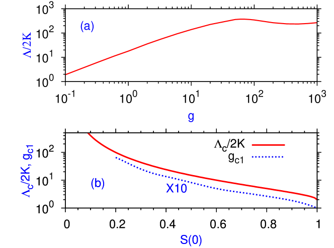
Figure 1: (a) The function $\Lambda/2K$ versus $g$ obtained using two-mode functions (10). (b) The critical $\Lambda_{c}/2K$ and $g_{c1}$ versus $S(0)$ from (9) and (10) for $\theta(0)=0$.

In the two-mode model [7, 11] a single-channel BEC wave function $\phi(x,t)$ of (3) is decomposed as [7]

$$\phi(x,t)=\psi_{1}(t)\Phi_{1}(x)+\psi_{2}(t)\Phi_{2}(x),$$ (4)

where spatial modes $\Phi_{i}(x)(i=1,2)$ in the two wells are orthonormalized as $\int\Phi_{i}(x)\Phi_{j}(x)=\delta_{ij}$ and the functions $\psi_{i}(t)$ satisfy $|\psi_{1}(t)|^{2}+|\psi_{2}(t)|^{2}=1$. The functions $\psi_{i}(t)$ are complex and are separated into its real and imaginary parts as $\psi_{i}(t)=|\psi_{i}(t)|\exp(i\theta_{i})$. A population imbalance

$$S(t)\equiv(|\psi_{1}(t)|^{2}-|\psi_{2}(t)|^{2})/(|\psi_{1}(t)|^{2}+|\psi_{2}(t)|^{2})=(|\psi_{1}(t)|^{2}-|\psi_{2}(t)|^{2})$$ (5)

and phase difference $\theta\equiv\theta_{2}-\theta_{1}$ then serve as a pair of conjugate variables. The approximation (4) is then substituted in (3), and after some straightforward algebra we obtain [7]

$$\dot{S}(t)=-2K\sqrt{1-S^{2}(t)}\sin\theta(t),$$ (6)

$$\dot{\theta}(t)=\Lambda S(t)+2K\frac{S(t)}{\sqrt{1-S^{2}(t)}}\cos\theta(t),$$ (7)

where $\Lambda=g\int dx\Phi^{4}_{i}(x)$ and

$$K=-\int dx\Phi_{1}(x)\left[-\frac{1}{2}\frac{d^{2}}{dx^{2}}+V(x)\right]\Phi_{2}(x).$$ (8)

The two-mode equations (6) and (7) are the Hamilton equations [7] $\dot{S}=-{\partial H}/{\partial\theta},\dot{\theta}=-{\partial H}/{\partial S},$ for Hamiltonian $H={\Lambda}S^{2}(t)/2-2K\sqrt{1-S^{2}(t)}\cos\theta(t).$ The transition from Josephson oscillation to self trapping happens at $H=2K$ above a critical $\Lambda=\Lambda_{c}$ for [7]

$$\frac{\Lambda}{2K}>\frac{\Lambda_{c}}{2K}\equiv\frac{2+2\sqrt{1-S^{2}(0)}\cos\theta(0)}{S^{2}(0)}.$$ (9)

To perform a numerical calculation using the two-mode model we choose the mode functions as [7]

$$\Phi_{1,2}(x)=[\Phi_{+}(x)\pm\Phi_{-}(x)]/\sqrt{2},$$ (10)

with the property $\Phi_{1}(-x)=\Phi_{2}(x)$, where $\Phi_{\pm}(x)$ are the symmetric ground and antisymmetric first excited state of (3) with potential (2) with an appropriate $g$. The parameters of potential (2) are taken as $A=16$ and $\kappa=10$ (used in most of numerical calculations below).

Now we calculate the quantity $\Lambda/2K$ for different $g$ and plot in figure 1 (a). Then a critical $\Lambda_{c}$ for self trapping is obtained from (9) and plotted in figure 1 (b) versus $S(0)$ for $\theta(0)=0$. From figure 1 (b) we see that for $S(0)=0.1$, the critical $\Lambda_{c}/2K\sim 400$. From figure 1 (a) we see that this $\Lambda/2K$ is never attained for any nonlinearity $g$. Hence no self trapping can be obtained for $S(0)<0.1$. For $S(0)>0.2$, the critical $\Lambda_{c}/2K$ for self trapping as obtained from figure 1 (b), can be attained for $g>g_{1c}$ as seen in figure 1 (a). However, with further increase of $g$, $\Lambda$ continues to be always greater than $\Lambda_{c}$ and the self trapping is never destroyed with the increase of $g$. In our numerical study we shall find that the self trapping is destroyed with the increase of $g$. This is reasonable as the two-mode model with the neglect of overlap integrals between the mode functions $\Phi_{1,2}(x)$ is expected to be valid for small $g$ only. A critical nonlinearity for self trapping $g_{1c}$ for $\theta(0)=0$ and different $S(0)$ is then obtained from the results of $\Lambda/2K-g$ and $\Lambda_{c}/2K-S(0)$ plots in figures 1 (a) and (b) and is also plotted in figure 1 (b).

3 Numerical results for Double-Well (DW) potential

The GP equations are solved numerically using the Crank-Nicolson scheme [27, 28] with space and time steps 0.025 and 0.0002, respectively, by real-time propagation with FORTRAN programs provided in [27].

3.1 Single-Channel BEC

Here we consider DW (2) with $A=16$ and $\kappa=10$, as in some previous studies [9, 10] on self trapping. In numerical simulation we create an initial state with a fixed population imbalance $S(0)$, by looking for the ground state at $x=x_{0}$ of the following asymmetric well [9]

$$U(x)=(x-x_{0})^{2}/2+Ae^{-\kappa x^{2}}.$$ (11)

The initial $S(0)$ is achieved by varying the parameter $x_{0}$ in (11) [9]. Once this initial state is created, $x_{0}$ is reduced to zero so that DW (11) reduces to DW (2) with $x_{0}=0$. If $x_{0}$ is reduced slowly during time evolution, the initial asymmetric state relaxes to a symmetric stationary state of DW (2) and there is no self trapping. On the other hand if $x_{0}$ is reduced quickly, there is always self trapping provided that $g$ lies in the appropriate window: $g_{1c}<g<g_{2c}$. This is shown in figure 2, where we plot the density at different $t$ after $x_{0}$ is reduced to zero during an interval $\Delta t=5,$ and 20. From figure 2 we find that there is self trapping for $\Delta t=5$ and no self trapping for $\Delta t=20$, when the asymmetric initial state relaxes to a final symmetric state. By actual substitution of the wave function of the self-trapped state in the time-independent GP equation we verify that there is no stationary state of the DW with this density. The present trapped wave function was generated from the ground state of DW (11) and is always positive with no node and the present self trapping is dynamical without any static counterpart.

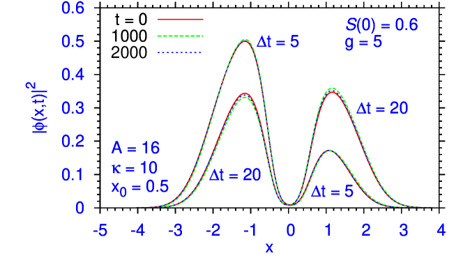
Figure 2: Density $|\phi(x,t)|^{2}$ versus $x$ at different $t$ when an initial state, created as the ground state of the asymmetric DW (11), is allowed to evolve in time while the asymmetric DW (11) is changed to the symmetric DW (2) by reducing $x_{0}$ to zero slowly in an interval of time $\Delta t=5,20.$ When the transition is quick ($\Delta t=5$) a permanent self trapping with an asymmetric profile emerges. For a slow transition ($\Delta t=20$), the system smoothly moves to the symmetric ground state of the symmetric DW (2) and there is no self trapping.

The self trapping is sensitive to $S(0)$. There is no self trapping for a small $S(0)(<0.1)$ (viz., two-mode model of section 2). In figure 3 (a) (upper panel) we plot $S(t)$ versus $t$ to illustrate the trapping and oscillation for different $g$ $(=1,10,100,1000)$ for $S(0)=0.3$. For $g=1$, there is Josephson oscillation with $\langle S(t)\rangle=0.$ For $g=10$ we have $\langle S(t)\rangle\sim 0.3$ insuring self trapping. As $g$ is further increased, the nonlinear term in the GP equation becomes much larger than the Gaussian wall $A\exp(-\kappa x^{2})$ in (2). Consequently, the DW appears like a single well and classical center-of-mass oscillation appears for a large $g$. For $g=100$ the oscillation is irregular because the Gaussian wall is not fully negligible. Finally, for $g=1000$ the Gaussian wall can be completely neglected and we have clean classical center-of-mass oscillation. The $S(t)$ versus $t$ plot for $S(0)=0.3$ and $g=10$ at large times is shown in the lower panel of figure 3 (a), where self trapping is confirmed up to $t=5000$ $-$ an interval much larger than tunneling time which is at best $\sim 100$. The evolution of $S(t)$ at large times $S(\infty)$ for different $S(0)$ as $g$ is increased is shown in figure 3 (b). A nonzero $S(\infty)$ ensures self trapping, which appears in the window: $g_{c1}<g<g_{c2}$. The prediction of the analytical two-mode model of section 2, from figure 1 (b), for $g_{c1}$ are shown by arrows in figure 3 (b) for $S(0)=0.3$ and 0.6 in good agreement with numerical simulation. It is noted that in all calculations reported here $g_{c2}<100$ $-$ a medium value of nonlinearity where the mean-field GP description is well justified. For larger values of nonlinearities, beyond mean-field corrections to the GP equation [29] could be relevant [30]. However, we expect the general conclusions of this study to remain valid for the present set of parameters.

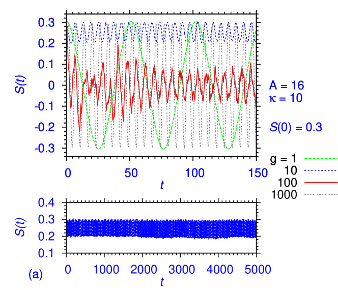
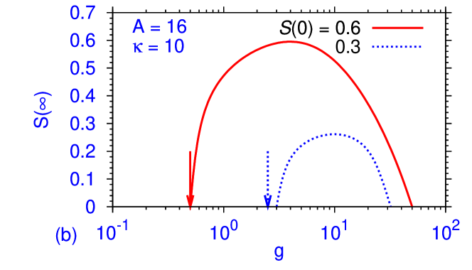
Figure 3: (a) (upper panel) Population imbalance $S(t)$ versus $t$ for $S(0)=0.3$ in DW (2). (lower panel) Long-time $S(t)$ versus $t$ for $g=10$. (b) Average population imbalance at large time $S(\infty)$ versus $g$ for $S(0)=0.3$ and 0.6. The arrows are results for $g_{c1}$ from figure 1 (b).

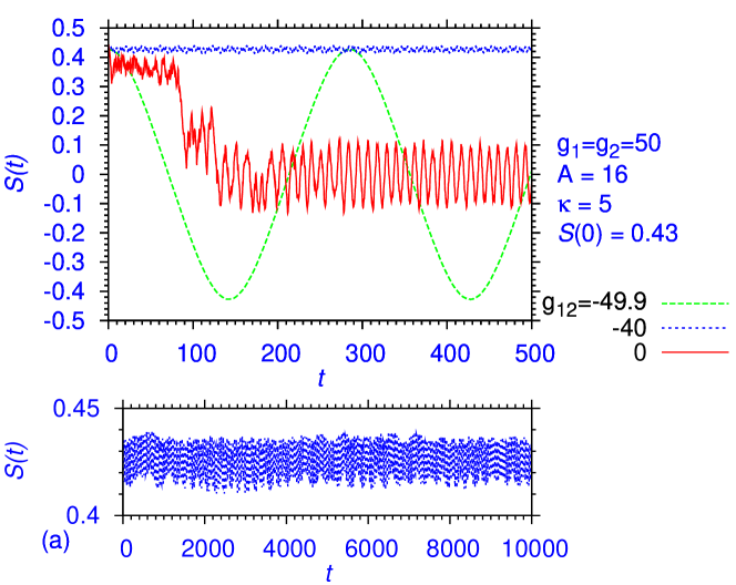
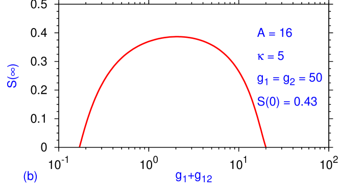
Figure 4: (a) (upper panel) Population imbalance $S(t)$ versus $t$ for a binary BEC with $S(0)=0.43$ and nonlinearities $g_{1}=g_{2}=50$ and $g_{12}=0,-40$ and $-49.9$ with DW (2). (lower panel) Long-time $S(t)$ versus $t$ dynamics for $g_{12}=-40$. (b) Average population imbalance $S(\infty)$ at large time versus effective nonlinearity $g_{1}+g_{12}$ for $S(0)=0.43$.

3.2 Binary BEC

We consider the self trapping of a binary BEC in a DW for $g_{i}>g_{c2}$ and $g_{i}<g_{c1}$. In both cases no self trapping is possible for zero interspecies interaction ($g_{12}=0$). Of these, for $g_{i}<g_{c1}$ we need a repulsive (positive) $g_{12}$ to make both components sufficiently repulsive to have self trapping. But this case usually leads to a uninteresting stationary phase separated configuration [31] with the first species occupying the first well of the DW and the second species occupying the second well. A more interesting situation emerges for $g_{i}>g_{c2}$, when we require an attractive (negative) $g_{12}$ to make both components appropriately repulsive to have self trapping. However, self trapping appears only for an intermediate $S(0)$ for an appropriate $g_{i}$ and $g_{12}$. To illustrate, we consider the symmetric case with $g_{1}=g_{2}=50$ in (1) and (2) and consider an attractive (negative) $g_{12}$. In the binary case, the self trapping is not so good for $\kappa=10$, while the barrier between the two wells in (2) is narrow and we take $\kappa=5$ in the numerical simulation. Permanent self trapping is found to occur for a narrow window of $S(0)$ around $S(0)=0.4$. For $S(0)>0.5$ and $S(0)<0.3$ self trapping for a small interval of time could be obtained.

The initial state with $S(0)=0.43$ for both components is created using DW (11) and reducing $x_{0}$ to zero. In the upper panel of figure 4 (a), we plot $S(t)$ versus $t$ for both components for three values of $g_{12}$. For $g_{12}\geq 0$, no self trapping is possible and we are in the domain of irregular oscillation as shown for $g_{12}=0$. For an attractive $g_{12}$, there is permanent self trapping as illustrated for $g_{12}=-40$. With further increase of $|g_{12}|$ the self trapping disappears and regular sinusoidal Josephson oscillation appears as shown for $g_{12}=-49.9$ in figure 4 (a). The lower panel of figure 4 (a) illustrates the population imbalance $S(t)$ for $g_{12}=-40$ at large times, which confirms robust self trapping. In figure 4 (b) we plot $S(\infty)$ for both components versus $g_{1}+g_{12}$. In the symmetric case with $g_{1}=g_{2}$, the wave function of the two components are equal and the quantity $g_{1}+g_{12}$ is the effective nonlinearity of each component. Figure 4 (b) shows that self trapping occurs for the window of effective nonlinearity $0.2<g_{1}+g_{12}<20$ for $S(0)=0.43$. For any given initial population imbalance and for either sufficiently small or sufficiently large effective nonlinear interaction strength $g_{1}+g_{12}$, the system is in the oscillation regime. For small values of effective interaction one has Josephson oscillation and for large values of effective interaction one has the classical center-of-mass oscillation. For intermediate interaction strength, the system may make transition to self trapping for an appropriate $S(0)$.

4 Analytical formulation for Optical-Lattice (OL) potential

For an OL, Eqs. (1) and (3) remain valid but with the variables bearing the following relations to the corresponding physical observables [24]: $t=(\pi/L)^{2}(\hbar/m)t_{\mathrm{phys}},x=\hat{x}\pi/L,V_{0}=m(L/\pi\hbar)^{2}V_{ol},\{g_{i},g_{12}\}=(2NLm\omega_{\perp}/\pi\hbar)\{a_{i},a_{12}\},$ where $L$ the wavelength and $V_{0}$ the strength of OL potential: $V_{OL}(\hat{x})=-V_{0}\pi^{2}\hbar^{2}/(mL^{2})\cos(2\pi\hat{x}/L)$. The dimensionless OL potential is given by

$$V(x)=-V_{0}\cos(2x).$$ (12)

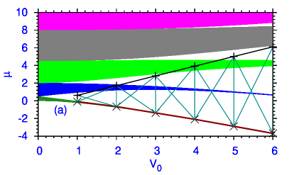
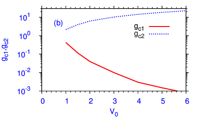
Figure 5: (a) Chemical potential $\mu$ versus $V_{0}$ showing the bands (shaded area) and gaps (white area) for OL (12). The hatched area between the lower line with crosses and the upper line with pluses represents the variational domain of the appearance of Gaussian gap solitons. The full white area above the lower line with crosses denote the exact domain of the appearance of gap solitons. (b) The critical values $g_{c1}$ and $g_{c2}$ defining the window of nonlinearities of Gaussian gap solitons versus $V_{0}$.

To critically examine the self trapping in a OL where the BEC is localized in one of the sites of the OL, we present a Gaussian variational analysis. The stationary state is described by (3) with the time derivative term $i\dot{\phi}$ replaced by $\mu\phi$ where $\mu$ is the chemical potential. The Lagrangian for that stationary equation is given by [19]

$$L=\int_{-\infty}^{\infty}\left[\mu\phi^{2}(x)-\phi_{x}^{2}(x)/2-g\phi^{4}(x)/2+V_{0}\cos(2x)\phi^{2}(x)\right]dx-\mu.$$ (13)

This Lagrangian can be analytically evaluated by considering a simple form for the wave function $\phi$. Using the Gaussian form [25] $\phi(x)=\pi^{-1/4}\sqrt{{\cal N}/w}\exp[-x^{2}/(2w^{2})]$ with ${\cal N}$ the norm and $w$ the width, the Lagrangian can be written as

$$L=\mu({\cal N}-1)-\frac{\cal N}{4w^{2}}+V_{0}{\cal N}\exp(-w^{2})-\frac{g{\cal N}^{2}}{2\sqrt{2\pi}w}.$$ (14)

The variational equations [25] $\partial L/\partial\mu=\partial L/\partial w=\partial L/\partial{\cal N}=0$ yield ${\cal N}=1$ and

$$1 + \frac{gw}{\sqrt{2\pi}}=4V_{0}w^{4}\exp(-w^{2}),$$ (15)

$$\mu = \frac{1}{4w^{2}}+\frac{g}{\sqrt{2\pi}w}-V_{0}\exp(-w^{2}),$$ (16)

which determine the width and the chemical potential. We have set ${\cal N}=1$ in (15) and (16) after derivation.

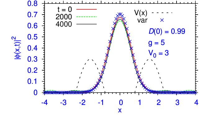
Figure 6: Density $|\phi(x,t)|^{2}$ versus $x$ at different $t$ when an initial Gaussian state with trapping measure $D(0)=0.99$ is released at $x=t=0$ on the OL. The variational result for the corresponding gap soliton is shown by crosses. The positive part of the potential is also shown in arbitrary units.

It is instructive to study the band and gap structure of the Schrödinger equation in the periodic OL potential (12): $\mu\phi(x)=-(1/2)\phi_{xx}(x)-V_{0}\cos(2x)\phi(x)$ [26]. In a periodic potential the quantum excitation spectrum of a system consists of bands and gaps. The bands allow unlocalized plane wave solution modulated by a periodic function with the same period as the periodic potential known as Bloch wave. The gaps permit localized solution [26]. However, the single-particle linear Schrödinger equation does not allow any solution in the gap. The band (shaded regions) and gap (white regions above the lowest shaded region) of the spectrum of the Schrödinger equation with OL potential (12) is shown in figure 5 (a). The nonlinear 1D GP equation (3) for repulsive interaction (positive $g$) permits localized solutions in the gaps, called gap solitons, where the chemical potential $\mu$ lies in the gap. In the gaps, localized gap solitons are possible in the presence of an appropriate nonlinearity $g$.

We now find the condition for a gap soliton for a positive (repulsive) $g$ by directly solving (15) and (16) for all $g$ and $V_{0}$. As $\mu$ tends to the upper edge of the lowest band, one has the lower limit $g_{c1}$ of the formation of a gap soliton, denoted by a line with crosses in figure 5 (a). As the repulsive nonlinearity $g$ is increased, (15) and (16) permit solution up to a maximum value $g_{c2}$ which determine the upper limit of the formation of a gap soliton denoted by the line with pluses in figure 5 (a). The area between the two lines determine the domain in which the Gaussian gap solutions are allowed. (Gap solitons of non-Gaussian shape, possibly occupying many OL sites, are possible in the whole white region above the lowest band gap in figure 5 (a).) The nonlinearities corresponding to these two lines can be calculated using (15) and (16) and yields the critical $g_{c1}$ and $g_{c2}$ for self trapping. These nonlinearities are plotted in figure 5 (b).

5 Numerical results for Optical-Lattice (OL) potential

5.1 Single-Channel BEC

The numerical simulation is started by releasing a Gaussian state in the center of the OL during time evolution of the GP equation. The width of the Gaussian is taken such that the initial state stays mostly in the central well of the OL. An estimate of self trapping is given by the following function called trapping measure

$$D(t)=\int_{-\pi/2}^{\pi/2}|\phi(x,t)|^{2}dx.$$ (17)

Here we note that $\pi$ is the wave length of the OL $-V_{0}\cos(2x)$. Hence the function $D(t)$ determines the matter inside a single OL site. In case of ideal self trapping in a single site $D(t)=1$, and $D(t)$ will tend to zero when self trapping is fully destroyed.

Self trapping occurs easily if the nonlinearity $g$ is appropriate for a Gaussian gap soliton (viz. figure 5). We take an initial Gaussian state with $D(0)=0.99$ and release it on the OL with $V_{0}=3$ and $g=5$. The density profile of the trapped state are shown in figure 6. The small dispersion of the density profile at different $t$ guarantees good self trapping. We also plot the density of the variational gap soliton, in good agreement with the self-trapped state, in figure 6.

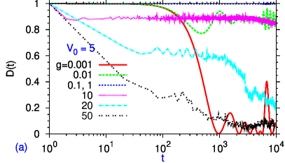
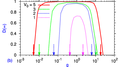
Figure 7: (a) Trapping measure $D(t)$ versus time $t$ for $V_{0}=5$ for different $g$. (b) Trapping measure at large time $D(\infty)$ versus $g$ for different $V_{0}=1,2,3,5$. The respective arrows represent nonlinearities $g_{c1}$ and $g_{c2}$ from figure 5 (b).

In Fig 7 (a) we plot $D(t)$ versus $t$ for $V_{0}=5$ and different $g$. For $g<10$, $D(t)$ remains close to 1 for $t<100$. However, if we continue to large $t(<10000)$ (a time much larger than the tunneling time of few hundred as in Fig 7 (a)), $D(t)$ remains close to 1 for a window of nonlinearity $0.01<g<10$ denoting permanent self trapping. For illustration, in figure 7 (b), we plot the trapping measure $D(t)$ at large times $D(\infty)$ versus $g$, where $D(\infty)$ is non-zero in the window $g_{c1}<g<g_{c2}$ corresponding to permanent self trapping and is zero outside showing no self trapping. In figure 7 (b) there are two arrows for each $V_{0}$ corresponding to $g_{c1}$ and $g_{c2}$ as obtained in figure 5 (b). The domain between the two arrows representing the region of allowed gap solitons (see, figure 5) agrees well with the domain of self trapping represented by non-zero $D(\infty)$ as seen in figure 7 (b). From this fact and also from the proximity of the variational solution for density of a gap soliton with that for the numerical self-trapped state in figure 6, we conclude that the self trapped state represents small oscillation of a stable gap soliton. In this connection, the finding in Ref. [13], that a self-trapped state in an OL is always temporary, is not fully to the point. They missed the fact that for the window of nonlinearity $g_{c1}<g<g_{c2}$ the self trapping could occur in a stable stationary gap soliton state leading to a permanent trapping. Just outside this small window of nonlinearity a temporary self trapping at small times may take place, as can be seen in figure 7 (a).

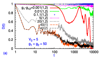
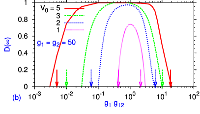
Figure 8: (a) Trapping measure $D(t)$ of a binary BEC versus time $t$ for different $g_{1}-g_{12}$. The curves are labeled by $g_{1}-g_{12}$ and the component number in parenthesis. (b) Trapping measure at large time $D(\infty)$ versus $g_{1}-g_{12}$ for different $V_{0}$. The arrows are $g_{c1}$ and $g_{c2}$ from figure 5 (b).

5.2 Binary BEC

To study self trapping of a binary BEC we consider large repulsive intraspecies nonlinearities $g_{1}=g_{2}=50,$ which do not allow self trapping for zero interspecies interaction $g_{12}=0$ for $V_{0}=1,2,3,5,$ as seen in figures 7 (a) and (b). If we introduce an attractive (negative) interspecies interaction $g_{12}$, then in each channel the effective nonlinearity will be reduced and for a sufficiently large and attractive $g_{12}$ one can have self trapping. The trapping dynamics for this system is illustrated in figure 8 (a) where we plot trapping measure $D(t)$ versus $t$ for different $g_{12}$ and $V_{0}=5,g_{1}=g_{2}=50$. The results for the two components are practically the same in most cases. The self trapping appears for a small $(g_{1}+g_{12})(\approx 0.01)$ and disappears for large $(g_{1}+g_{12})(>10)$. In this symmetric binary BEC, $(g_{1}+g_{12})$ provides a good measure of the effective nonlinearity controlling self trapping. In figure 8 (b) we plot the trapping measure at large times $D(\infty)$ versus effective nonlinearity $g+g_{12}$ of the binary BEC for $V_{0}=1,2,3,5$. The plots of figures 7 (b) and 8 (b) are qualitatively quite similar, showing that $(g_{1}+g_{12})$ is a good measure of effective nonlinearity of the binary BEC. However, if $|g_{12}|$ is taken to be larger than $g$ then the effective nonlinearity becomes attractive corresponding to a negative $g_{1}+g_{12}$. This domain of nonlinearity corresponds to permanent symbiotic bright soliton [32] and consideration of self trapping is inappropriate.

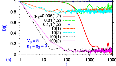
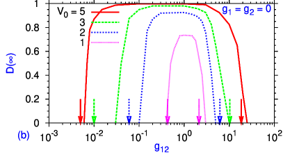
Figure 9: (a) Trapping measure $D(t)$ of a binary BEC versus time $t$ for $V_{0}=5$ and different $g_{12}$. Curves are labeled by $g_{12}$ and component number. (b) Trapping measure at large time $D(\infty)$ versus $g_{12}$ for different $V_{0}$. The arrows represent nonlinearities $g_{c1}$ and $g_{c2}$ from figure 5 (b).

Finally, we consider a binary BEC with small intraspecies nonlinearities and zero interspecies nonlinearity ($g_{12}=0$), that does not allow self trapping, as found in figures 7 (a) and (b). As an illustration we consider the zero values for the intraspecies nonlinearities: $g_{1}=g_{2}=0$. In the presence of appropriate repulsive interspecies nonlinearity ($g_{12}>0$), one can have self trapping as illustrated in figures 9 (a) and (b). In figure 9 (a) we plot the trapping measure $D(t)$ versus $t$ for different repulsive (positive) interspecies nonlinearity $g_{12}$ and $V_{0}=5,g_{1}=g_{2}=0$. In this case $g_{12}$ plays the role of effective interaction. There is a window of $g_{12}$ values $g_{c1}<g_{12}<g_{c2}$ with $g_{c1}\approx 0.01$ and $g_{c2}\approx 10$, where permanent self trapping can be achieved. In figure 9 (b) we plot large-time trapping measure $D(\infty)$ versus $g_{12}$ for different $V_{0}$ and $g_{1}=g_{2}=0$. Qualitatively, this plot is quite similar to those in figures 7 (b) and 8 (b) showing the universal nature of these plots.

6 Summary and Discussion

We demonstrated that self trapping of a BEC or a binary BEC without interspecies interaction in OL and DW occurs for a window of repulsive intraspecies nonlinearity $g$ ($g_{c1}<g<g_{c2}$), where $g_{c1}$ and $g_{c2}$ depends on the trap parameters. For a binary BEC with the intraspecies nonlinearities outside this window, a self trapping can be induced by a non-zero interspecies nonlinearity $g_{12}$ such that the effective nonlinearities fall in this window. For intraspecies nonlinearities $g_{i}$ below $g_{c1}$ ($g_{i}<g_{c1}$), this is achieved by an appropriate repulsive (positive) $g_{12}$. For intraspecies nonlinearities $g_{i}$ above $g_{c2}$ ($g_{i}>g_{c2}$), one can have self trapping by introducing an appropriate attractive (negative) $g_{12}$. In case of self trapping in an OL, the permanently self trapped state represents breathing oscillation of a stable stationary gap soliton. On the other hand, the self trapping in a DW is purely a dynamical phenomenon without any underlying stationary state. However, the self trapping of a BEC and a binary BEC in both DW and OL could be permanent.

In previous studies of self trapping of a BEC, the existence of a lower limit $g_{c1}$ of nonlinearity was noted [2, 7, 13, 14]. However, the disappearance of self trapping above an upper limit was not realized. (A similar upper limit appeared in a study of a Fermi superfluid in a DW [9].) In a previous study of self trapping in an OL, in contradiction with the present investigation, it was concluded that self trapping was always transient and should disappear at large $t$ [13].

The principal findings of this critical study of self trapping are the following. (a) The self-trapped states in an OL potential are essentially the stationary gap solitons. The self trapping in DW potential is entirely dynamical in nature and there are no stationary states in this case, such as the gap solitons of the OL potential. (There is no periodic potential and no band and band gap, specially for the case of a DW with a shallow barrier, which we shall study here.) It was generally believed that self trapping in both OL and DW potentials are dynamical in nature. (b) Self trapping is stopped beyond an upper limit of interaction in both cases. (c) In case of coupled systems with inter-species interaction self trapping is possible for domain of intra-species atomic interaction where no self trapping is allowed in uncoupled systems.

In the experiment of self trapping in an OL and in related theoretical studies a localized state over tens of OL sites [13, 14] was considered in contrast to that in predominantly a single OL site. Such states extended over multiple OL sites could possibly be a combination of multiple compact gap solitons. In another study, such states have been suggested to be a new type of spatially extended state in the gap [21]. The compact self trapped state on OL considered in this paper are different from the spatially extended states considered in other studies. Nevertheless, with the present experimental control over a BEC, it would be possible to study self trapping of the compact states on OL as considered in this paper.

References

- [1] Görlitz et al. A 2001 Phys. Rev. Lett. 87 130402
- [2] Albiez M, Gati R, Folling J, Hunsmann S, Cristiani M and Oberthaler M K 2005 Phys. Rev. Lett. 95 010402 Gati R and Oberthaler M K 2007 J. Phys. B: At. Mol. Opt. Phys.40 R61
- [3] Kastberg A, Phillips W D, Rolston S L, Spreeuw R J C and Jessen P S 1995 Phys. Rev. Lett.74 1542
- [4] Roati G et al. 2008 Nature 453 895 Khaykovich L et al. 2002 Science 256 1290
- [5] Cataliotti F S et al. 2001 Science 293 843
- [6] Javanainen J 1986 Phys. Rev. Lett.57 3164 Williams J E 2001 Phys. Rev. A 64 013610 Giovanazzi S, Smerzi A and Fantoni S 2000 Phys. Rev. Lett. 84 4521 Adhikari S K 2005 Phys. Rev. A 72 013619 Adhikari S K 2003 Eur. Phys. J. D 25 161 Morales-Molina L and Gong J B 2008 Phys. Rev. A 78 041403(R)
- [7] Smerzi A, Fantoni S, Giovanazzi S and Shenoy S R 1997 Phys. Rev. Lett.79 4950 (1997) Trombettoni A and Smerzi A 2001 Phys. Rev. Lett.86 2353 Raghavan S, Smerzi A, Fantoni S and Shenoy S R 1999 Phys. Rev. A 59 620
- [8] Ananikian D and Bergeman T 2006 Phys. Rev.A 73 013604 Ottaviani C, Ahufinger V, Corbalán R and Mompart J 2010 Phys. Rev.A 81 043621 Juliá-Díaz B, Dagnino D, Lewenstein M, Martorell J and Polls A 2010 Phys. Rev.A 81 023615 Lu L H and Li Y Q 2009 Phys. Rev. A 80 033619 Martinez M T, Posazhennikova A and Kroha J 2009 Phys. Rev. Lett.103 105302 Shchesnovich V S and Trippenbach M 2008 Phys. Rev. A 78 023611 Wang W, Fu L B and Yi X X 2007 Phys. Rev.A 75 045601 Fu L B and Liu J 2006 Phys. Rev. A 74 063614 Holthaus M 2001 Phys. Rev. A 64 011601
- [9] Adhikari S K, Lu H and Pu H 2009 Phys. Rev. A 80 063607
- [10] Xiong B, Gong J, Pu H, Bao W and Li B 2009 Phys. Rev. A 79 013626
- [11] Milburn G J et al. 1997 Phys. Rev. A 55 4318
- [12] Liu B, Fu L-B, Yang S-P and Liu J 2007 Phys. Rev. A 75 033601
- [13] Wang B, Fu P, Liu J and Wu B 2006 Phys. Rev. A 74 063610
- [14] Xue J K, Zhang A X and Liu J 2008 Phys. Rev. A 77 013602 Rosenkranz M, Jaksch D, Lim F Y and Bao W 2008 Phys. Rev. A 77 063607
- [15] Zhang W, Walls D F and Sanders B C 1994 Phys. Rev. Lett.72 60 Zhang W, Sanders B C and Tan W 1997 Phys. Rev.A 56 1433
- [16] Ostrovskaya E A et al. 2000 Phys. Rev. A 61 031601(R)
- [17] Billy J et al. 2008 Nature 453 891 Adhikari S K and Salasnich L 2009 Phys. Rev. A 80 023606 Adhikari S K 2010 Phys. Rev. A 81 043636 Modugno M 2009 New J. Phys. 11 033023 Cheng Y S and Adhikari S K 2010 Phys. Rev. A 81 023620 Cheng Y S and Adhikari S K 2011 Phys. Rev. A 83 Cheng Y S and Adhikari S K 2010 Phys. Rev. A 82 013631 Cheng Y S and Adhikari S K 2010 Laser Phys. Lett. 7 824 Larcher M, Dalfovo F and Modugno M 2009 Phys. Rev. A 80 053606
- [18] Eiermann B et al. 2004 Phys. Rev. Lett.92 230401 Morsch O and Oberthaler M 2006 Rev. Mod. Phys. 78 179
- [19] Adhikari S K and Malomed B A 2007 Europhys. Lett. 79 50003
- [20] Ostrovskaya E A and Kivshar Y S Phys. Rev. Lett. 90 160407
- [21] Alexander T J, Ostrovskaya E A Kivshar Y S 2006 Phys. Rev. Lett.96 040401
- [22] Zwierlein M W, Abo-Shaeer J R, Schirotzek A, Schunck C H and Ketterle W 2005 Nature 435 1047
- [23] Salasnich L, Parola A and Reatto L 2002 Phys. Rev. A 65 043614 Muñoz Mateo A and Delgado V 2008 Phys. Rev. A 77 013617 (2008) Buitrago C A G and Adhikari S K 2009 J. Phys. B: At. Mol. Opt. Phys.42 215306
- [24] Adhikari S K and Malomed B A 2009 Phys. Rev. A 79 015602
- [25] PerezGarcia V M, Michinel H, Cirac J I et al. 1997 Phys. Rev. A 56 1424
- [26] Kittel C 1996 Introduction to solid state physics, 7th Ed (New York, Wiley)
- [27] Muruganandam P and Adhikari S K 2009 Comput. Phys. Commun. 180 1888
- [28] Muruganandam P and Adhikari S K 2003 J. Phys. B: At. Mol. Opt. Phys.36 2501 Adhikari S K and Muruganandam P 2002 J. Phys. B: At. Mol. Opt. Phys.35 2831
- [29] Adhikari S K and Salasnich L 2008 Phys. Rev.A 77 033618 Adhikari S K and Salasnich L 2008 Phys. Rev.A 78 043616
- [30] Sakmann K, Streltsov A I, Alon O E and Cederbaum L S 2009 Phys. Rev. Lett.103 220601 Zöllner S, Meyer H.-D. and Schmelcher P 2008 Phys. Rev. Lett.100 040401 Rigol M, Rousseau V, Scalettar R T and Singh R R P 2005 Phys. Rev. Lett.95 110402
- [31] Riboli F and Modugno M 2002 Phys. Rev. A 65 063614
- [32] Adhikari S K 2005 Phys. Lett. A 346 179 Perez-Garcia V M and Beitia J B 2005 Phys. Rev. A 72 033620