Critical behavior and universality in Lévy spin glasses

Abstract

Using large-scale Monte Carlo simulations that combine parallel tempering with specialized cluster updates, we show that Ising spin glasses with Lévy-distributed interactions share the same universality class as Ising spin glasses with Gaussian or bimodal-distributed interactions. Corrections to scaling are large for Lévy spin glasses. In order to overcome these and show that the critical exponents agree with the bimodal and Gaussian case, we perform an extended scaling of the two-point finite size correlation length and the spin-glass susceptibility. Furthermore, we compute the critical temperature and compare its dependence on the disorder distribution width to recent analytical predictions [J. Stat. Mech. (2008) P04006].

I Introduction

Although universality has been established for many systems without disorder and frustration, there are still skeptics that question this cornerstone of the theory of statistical mechanics when applied to disordered spin systems with frustrated interactions. According to universality, the values of quantities such as critical exponents, do not depend on microscopic details of the model, but only on e.g., the space dimension and the symmetry of the order parameter. Arguments based on high-temperature series expansionsDaboul et al. (2004) support universality and there is no a priori reason why systems with both disorder and frustration, such as spin glasses,Binder and Young (1986) might not show universal features. However, numerical studies are difficultOgielski and Morgenstern (1985); Ogielski (1985); McMillan (1985); Singh and Chakravarty (1986); Bray and Moore (1985); Bhatt and Young (1985, 1988); Kawashima and Young (1996); Bernardi et al. (1996); Iñiguez et al. (1996); Berg and Janke (1998); Marinari et al. (1998); Palassini and Caracciolo (1999); Mari and Campbell (1999); Ballesteros et al. (2000); Mari and Campbell (2001, 2002); Nakamura et al. (2003); Pleimling and Campbell (2005); Jörg (2006); Ostilli (2006); Campbell et al. (2006); Toldin et al. (2006); Katzgraber et al. (2006); Hasenbusch et al. (2008); Romá (2010) and suffer from strong corrections to scaling. Therefore, there is still debateBernardi et al. (1996); Mari and Campbell (1999, 2001); Henkel and Pleimling (2005); Pleimling and Campbell (2005) for some model systems if the shape of the disorder distribution can influence the universality class of the system.

Although it is now well established that universality is not violated for nearest-neighbor spin glasses with compact disorder distributions (e.g., Gaussian or bimodal),Katzgraber et al. (2006); Hasenbusch et al. (2008); Jörg (2006) some studies suggest that this might not be the case when the disorder distributions are broad.Mari and Campbell (2001) If the spin interactions are drawn from a Gaussian or bimodal distribution the probability to have extremely large interactions is very small. It is, however, unclear if strong couplings between the spins change the universality class of the system. Selecting the interactions between the spins from a Lévy distribution allows one to continuously tune the probability to have very strong bonds in the system. In particular, for $\alpha<2$ (see below for details) the Lévy distribution has broad tails and thus the probability to have a strong bond between two spins is large, especially in the limit $\alpha\to 1$.

Using large-scale Monte Carlo simulations that combine parallel tempering with specialized cluster moves,Janzen et al. (2008) as well as extended scaling techniques,Campbell et al. (2006) our results show that Lévy spin glasses do obey universality for the system sizes studied. Our estimates of the critical exponents agree within error bars with the best known estimatesKatzgraber et al. (2006); Hasenbusch et al. (2008) for Gaussian and bimodal disorder. Furthermore, we probe recent analytical predictionsJanzen et al. (2008) made for the critical temperature of Lévy spin glasses as a function of the disorder distribution width.

The paper is structured as follows: In Sec. II we introduce the model studied, as well as the measured observables. Section III outlines the special (cluster) algorithm used to treat strong interactions in the Lévy spin glass, the finite-size scaling analysis, and how we estimate the critical temperature, followed by results presented in Sec. IV, as well as concluding remarks.

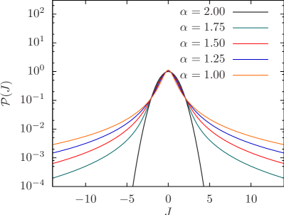
Figure 1: (Color online) Lévy distribution ${\mathcal{P}}(J)$ for the different values of the shape parameter $\alpha$ and $c=1/\sqrt{2}$, as studied here. In particular, for $\alpha=2$ a Gaussian distribution is recovered. For $1\leqslant\alpha<2$ the distribution is fat-tailed, as can be seen in the linear-log plot.

II Model and Observables

We study the critical behavior of the Edwards-Anderson Ising spin glassEdwards and Anderson (1975) with Lévy-distributed interactions, i.e.,

$${\mathcal{H}}=-\sum_{\langle i,j\rangle}J_{ij}S_{i}S_{j},$$ (1)

where the sites $i$ lie on a three-dimensional cubic lattice of size $N=L^{3}$, $L$ the linear dimension, and the spins $S_{i}$ can take the values $\pm 1$. Periodic boundary conditions are used to reduce corrections to scaling. The sum is over nearest neighbors and the interactions $J_{ij}$ are independent random variables taken from a Lévy distribution with zero mean and $c=1/\sqrt{2}$ defined through the characteristic function $\phi(t)$ as

$${\mathcal{P}}(J)=\frac{1}{2\pi}\int_{-\infty}^{+\infty}dt\phi(t)e^{-itJ}=\frac{1}{2\pi}\int_{-\infty}^{+\infty}dte^{-itJ-|ct|^{\alpha}}.$$ (2)

The parameter $\alpha$ influences the shape of the distribution and, in particular, the width of the tails. For $\alpha=2$ Eq. (2) reduces to a Gaussian with variance $\sigma=\sqrt{2}c$. When $1\leqslant\alpha<2$ the tail of the distribution decays as a power law, as seen in Fig. 1. In this case, exchange interactions with very large values can occur, albeit with small probability. However, such strong interactions form “dimers” of spins that cannot be flipped with standard Monte Carlo methods.Hartmann and Rieger (2001) For decreasing $\alpha$ the probability to have dimers grows, as well as the average of the maximum exchange interaction value.

To test universality, at least two independent critical exponents need to be computed. Therefore, in the simulations, we measure the following quantities.

The spin overlap $q$ is defined as

$$q=\frac{1}{N}\sum_{i}S_{i}^{(1)}S_{i}^{(2)},$$ (3)

where $(1)$ and $(2)$ are two copies of the system with identical disorder. Using $q$ we define the Binder ratioBinder (1981) $g$ via

$$g=\frac{1}{2}\left(3-\frac{\left[\langle q^{4}\rangle\right]_{\rm av}}{\left[\langle q^{2}\rangle\right]_{\rm av}^{2}}\right)\sim{\tilde{G}}[L^{1/\nu}(T-T_{c})],$$ (4)

where $\langle\cdots\rangle$ represents a thermal average and $[\cdots]_{\rm av}$ an average over the disorder. The Binder ratio is a dimensionless function $\tilde{G}$, i.e., data for different system sizes cross at a putative transition temperature $T_{c}$. A finite-size scaling analysis of the universal functionPrivman and Fisher (1984) $\tilde{G}$ allows one to determine the critical exponent $\nu$ for the correlation length.

The spin-glass susceptibility $\chi_{\rm SG}$ is defined as

$$\chi_{\rm SG}=N\left[\langle q^{2}\rangle\right]_{\rm av}\sim L^{2-\eta}\tilde{C}[L^{1/\nu}(T-T_{c})].$$ (5)

A finite-size scaling analysis of the susceptibility thus permits the calculation of the critical exponent $\eta$. However, a simple scaling analysis of the spin-glass susceptibility suffers from strong corrections to scalingKatzgraber et al. (2006) and therefore an extended scalingCampbell et al. (2006) is performed below where the scaling function incorporates corrections derived from the resummation of a high-temperature series expansion.

Finally, we measure the two-point finite-size correlation length.Palassini and Caracciolo (1999); Ballesteros et al. (2000) To do so we introduce the wave-vector-dependent spin-glass susceptibility

$$\chi_{\rm SG}\left({\bf k}\right)=\frac{1}{N}\sum_{i,j}\left[\langle S_{i}S_{j}\rangle^{2}\right]_{av}e^{\text{i}{\bf k}\left({\bf R}_{i}-{\bf R}_{j}\right)}.$$ (6)

The two-point finite-size correlation length $\xi_{L}$ is then given by

$$\xi_{L}=\frac{1}{2\sin\left(k_{\rm min}/2\right)}\sqrt{\frac{\chi_{\rm SG}({\bf 0})}{\chi_{\rm SG}({\bf k}_{\rm min})}-1},$$ (7)

where ${\bf k}_{\rm min}=(2\pi/L,0,0)$. It scales as

$$\frac{\xi_{L}}{L}=\tilde{X}[L^{1/\nu}(T-T_{c})],$$ (8)

i.e., whenever $T=T_{c}$ data for different system sizes cross at one point, up to corrections to scaling.Hasenbusch et al. (2008)

III Numerical Details

To test for universal behavior a detailed numerical study needs to be performed where one has to ensure that the data are in thermal equilibrium. For this purpose we use a special cluster algorithm that ensures that spin dimers flip in reasonable simulation times. In addition, we describe the data analysis used.

III.1 Algorithm

The simulations are done using the parallel tempering Monte Carlo methodHukushima and Nemoto (1996) combined with a special cluster flip algorithmJanzen et al. (2008) that ensures ergodic behavior even in the presence of excessively strong exchange interactions between few spins.

Because the Lévy distribution has power-law decaying tails, for certain values of the parameter $\alpha$ the exchange interactions $J_{ij}$ can be very large. If two spins have a strong interaction they will be virtually “frozen” under single-spin-flip dynamics. To avoid extremely long equilibration times, at the beginning of each simulation different sets of clusters $C_{n}$ are generated.Janzen et al. (2008) The generation of the sets $C_{n}$ is done the following way:

1. Set $J^{0}_{\rm min}=T_{\rm max}/4$, where $T_{\rm max}$ is the maximal temperature from the simulated temperature set.

2. The clusters in set $C_{n}$ consist of spins connected by bonds that satisfy $|J_{ij}|>J^{n}_{\rm min}$.

3. The cluster set $C_{n}$ is stored if $C_{n}\neq C_{n-1}$ (or if $n=0$).

4. $J^{n}_{\rm min}$ is iteratively incremented by one ($J^{n+1}_{\rm min}=J^{n}_{\rm min}+1$). The procedure is repeated initiating from step two until $C_{n}$ consists only of clusters of size $2$. During the procedure all clusters are stored.

One Monte Carlo sweep consists of the following procedure: Each spin of the system is picked once. After having picked the spin, a single-spin flip is performed with probability $p=0.75$ (empirically we find that for $p\sim 0.75$ equilibration is fastest), otherwise a cluster move is done. In particular:

• The single spin flip is done with the Metropolis probability $\min\{1,\exp(-\Delta E/T)\}$, where $\Delta E$ is the energy difference between the current configuration and the configuration with the spin flipped.

• The cluster flip algorithm works as follows: One cluster from all sets is randomly (uniformly) picked and flipped with the Metropolis probability $\min\{1,\exp(-\Delta E/T)\}$, where $\Delta E$ is the difference between the energy of the actual configuration and the configuration with the cluster flipped. The cluster flip is independent of the orientation of the spins in the cluster, i.e., the clusters contain only spin indices, such that each spin in the cluster can change the direction by other update steps.

Note that typical cluster sizes range from $2$ –$20$ spins.

Because the equilibration test for Gaussian disorderKatzgraber et al. (2001) does not work when the disorder is Lévy distributed, the equilibration is monitored by logarithmic binning. All measured observables (and their higher moments) are recorded as a function of simulation time. Once the last four bins agree within error bars the system is deemed to be in thermal equilibrium. If this test is not passed, the simulation time is increased by a factor of 2 until this is the case. Simulation parameters are summarized in Table 1.

Table 1: Parameters of the simulations for different $\alpha$ values. $N_{\rm sa}$ is the number of samples, $N_{\rm sw}$ is the total number of Monte Carlo sweeps used for equilibration (the same amount is used for measurement), $T_{\rm min}$ is the lowest temperature simulated, $T_{\rm max}$ is the highest temperature simulated, and $N_{T}$ is the number of temperatures used in the parallel tempering method for each system size $L$.

$\alpha$	$L$	$N_{\rm sa}$	$N_{\rm sw}$	$T_{\rm min}$	$T_{\rm max}$	$N_{T}$
$1.00$	$4$	$6000$	$65536$	$1.112$	$2.000$	$12$
$1.00$	$6$	$4830$	$252144$	$1.112$	$2.000$	$12$
$1.00$	$8$	$3737$	$1048576$	$1.112$	$2.000$	$12$
$1.00$	$10$	$3400$	$4194304$	$1.112$	$2.000$	$12$
$1.00$	$12$	$3995$	$16777216$	$1.112$	$2.000$	$12$
$1.00$	$14$	$1118$	$33554432$	$1.305$	$1.896$	$8$
$1.25$	$4$	$5600$	$65536$	$0.898$	$1.704$	$13$
$1.25$	$6$	$5082$	$262144$	$0.898$	$1.704$	$13$
$1.25$	$8$	$4165$	$1048576$	$0.898$	$1.704$	$13$
$1.25$	$10$	$4995$	$2097152$	$0.898$	$1.704$	$13$
$1.25$	$12$	$2998$	$16777216$	$0.898$	$1.704$	$13$
$1.50$	$4$	$5040$	$65536$	$0.726$	$1.452$	$14$
$1.50$	$6$	$4958$	$262144$	$0.726$	$1.452$	$14$
$1.50$	$8$	$5083$	$1048576$	$0.726$	$1.452$	$14$
$1.50$	$10$	$3014$	$2097152$	$0.726$	$1.452$	$14$
$1.50$	$12$	$3006$	$16777216$	$0.726$	$1.452$	$14$
$1.75$	$4$	$5040$	$65536$	$0.618$	$1.305$	$15$
$1.75$	$6$	$5016$	$262144$	$0.618$	$1.305$	$15$
$1.75$	$8$	$4592$	$1048576$	$0.618$	$1.305$	$15$
$1.75$	$10$	$4794$	$2097152$	$0.618$	$1.305$	$15$
$1.75$	$12$	$3999$	$16777216$	$0.618$	$1.305$	$15$

III.2 Finite-size scaling analysis

To gain insights on the strength of the corrections to scaling, we can compare two dimensionless quantities,Katzgraber et al. (2006); Jörg (2006) the correlation length $\xi_{L}/L$ and the Binder parameter $g$. By plotting $g[\xi_{L}(T,L)/L]$ there are no nonuniversal metric factors. Therefore, data for all system sizes simulated and a given parameter $\alpha$ should all collapse onto a universal function if there are no corrections to scaling. Data for $\alpha=1.25$ are shown in Figure 2 and illustrate that corrections are large for $L\lesssim 8$.

Furthermore, if two different models share the same critical exponent $\nu$, because no nonuniversal factors when plotting $g[\xi_{L}(T,L)/L]$ are present, all data should collapse onto a universal curve. In Fig. 2 we also show data for Gaussian disorder ($\alpha=2$) for a large system size ($L=24$).Katzgraber et al. (2006) Data for $\alpha=1.25$ and $L\gtrsim 8$ agree with the Gaussian case, thus illustrating that for a conventional scaling analysis only the largest system sizes should be included.

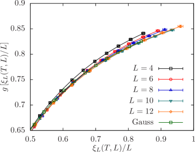
Figure 2: (Color online) Binder ratio $g$ as a function of the finite-size correlation length $\xi_{L}/L$ for several system sizes and for a Lévy parameter $\alpha=1.25$. Strong corrections to scaling are visible. The data for the largest system sizes simulated agree with the Gaussian case ($\alpha=2$, $L=24$, from Ref. Katzgraber et al., 2006).

We have attempted different scaling approaches,Jörg (2006); Katzgraber et al. (2006) as well as the inclusion of corrections to scaling.Hasenbusch et al. (2008) However, large system sizes are difficult to simulate for Lévy spin glasses and therefore we use the extended scaling techniqueCampbell et al. (2006) that allows us to include smaller system sizes in the scaling analysis.

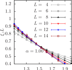
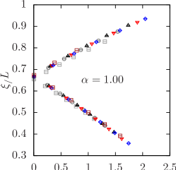
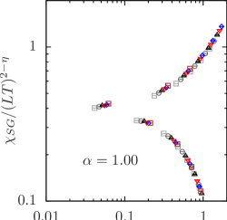
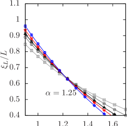
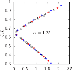
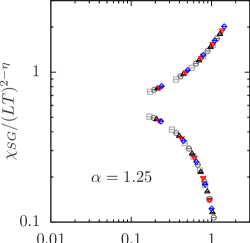
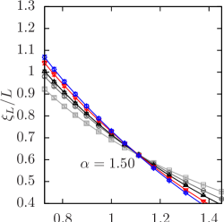
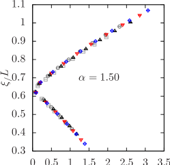
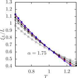
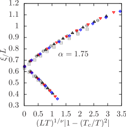
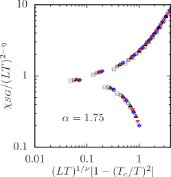
Figure 3: (Color online) Left: Two-point finite-size correlation length $\xi_{L}/L$ as a function of the temperature $T$ for different Lévy parameters $\alpha$. The data cross, thus signaling the presence of a transition. Center: Extended scaling of the two-point finite-size correlation length for different $\alpha$. Right: Extended scaling of the spin-glass susceptibility for different $\alpha$. The data scale very well and the critical exponents extracted from the scaling agree within error bars, thus suggesting that all systems share the same universality class. See Table 2 for the optimal scaling parameters.

Within the extended scaling frameworkCampbell et al. (2006) the standard scaling expression for the correlation length, Eq. (8), is replaced by

$$\frac{\xi_{L}}{L}\sim\tilde{X}[(LT)^{1/\nu}|1-(T/T_{c})^{2}|].$$ (9)

The aforementioned expression is derived by including a resummation of a high-temperature series expansion and therefore includes effects of corrections to scaling. Similarly, the scaling relation for the susceptibility, Eq. (5), is replaced by

$$\chi_{SG}(L,T)\sim(LT)^{2-\eta}\tilde{C}[(LT)^{1/\nu}|1-(T/T_{c})^{2}|].$$ (10)

We assume that the scaling function in Eq. (9) can be approximated by a third-order polynomial for temperatures larger than $T_{c}$, i.e., $\tilde{X}(x)=a+bx+cx^{2}+dx^{3}$ where $x=(LT)^{1/\nu}|1-(T/T_{c})^{2}|$, $T>T_{c}$ and perform a fit to the six parameters $a$, $b$, $c$, $d$, $T_{c}$ and $\nu$. A similar approach is used for the spin-glass susceptibility [Eq. (10)], for which there is a seventh parameter, the critical exponent $\eta$. Note that the extended scaling scheme only works for temperatures $T>T_{c}$. Therefore, we first perform a rough estimate of $T_{c}$ using conventional scaling methods. The nonlinear fit is performed with the statistics package R,R including system sizes $L\geqslant 6$. Error bars are determined using a bootstrap analysis.

To compute the error bars we apply the following procedure: For each system size $L$ and $N_{\rm sa}$ disorder realizations, a randomly selected bootstrap sample of $N_{\rm sa}$ disorder realizations is generated. With this random sample, an estimate of the different observables is computed for each temperature. We repeat this procedure $N_{\rm boot}=500$ times for each lattice size and then assemble $N_{\rm boot}$ complete data sets (each having results for every size) by combining the $i$-th bootstrap sample for each size for $i=1,\ldots,N_{\rm boot}$. The finite-size scaling fit described above is then carried out on each of these $N_{\rm boot}$ sets, thus obtaining $N_{\rm boot}$ estimates of the fit parameters. Because the bootstrap sampling is done with respect to the disorder realizations which are statistically independent, we can use a conventional bootstrap analysis to estimate statistical error bars on the fit parameters. These are comparable to the standard deviation among the $N_{\rm boot}$ bootstrap estimates.Katzgraber et al. (2006)

From the aforementioned finite-size scaling we can also extract the critical temperature $T_{c}(\alpha)$ to compare to analytical predictions. We use the critical temperature estimated using the extended scaling method for the correlation length [Eq. (9)] because corrections to scaling are smaller than for the spin-glass susceptibility. Furthermore, the bootstrap analysis requires one parameter less leading to smaller statistical errors.

IV Results

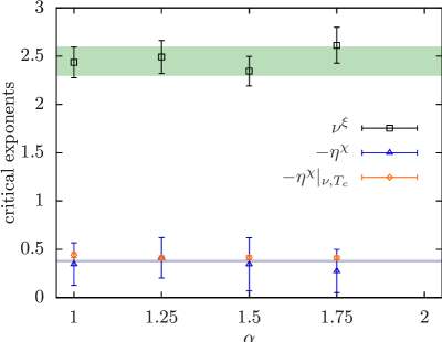
Figure 4: (Color online) Critical exponents $\eta$ and $\nu$ as a function of the Lévy parameter $\alpha$. The shaded areas correspond to the estimates for Bimodal disorder from Ref. Hasenbusch et al., 2008. The estimate for the critical exponent $\nu^{\xi}$ comes from an extended finite-size scaling analysis of the two-point correlation length. The estimates for the critical exponent $\eta$ are from two independent analyses of the spin-glass susceptibility. $\eta^{\chi}$ is computed from an extended finite-size scaling analysis where $\eta$, $\nu$, and $T_{c}$ are parameters, whereas $\eta^{\chi}|_{\nu,T_{c}}$ is computed by fixing $\nu=\nu^{\xi}$ and $T_{c}=T_{c}^{\xi}$ from the analysis of the two-point correlation length. For all values of $\alpha$ studied, the exponents $\nu^{\xi}$ and $\eta^{\chi}$ are in good agreement with the best-known estimates for the bimodal case. However, the estimate for $\eta^{\chi}|_{\nu,T_{c}}$ consistently lies above the best estimate for $\eta$ possibly due to strong corrections to scaling that we cannot account for, as well as systematic errors from the determination of $\nu^{\xi}$.Katzgraber et al. (2006)

Corrections to scaling for small systems of Lévy spin glasses with $1\leqslant\alpha<2$ are large (see Fig. 2). We attempt to scale the data using the extended scaling scheme, as shown in Fig. 3 (center and right columns). The left column shows the finite-size correlation length for different values of the parameter $\alpha$. In all cases the data cross at a transition temperature that decreases with increasing $\alpha$. In the center panels of Fig. 3 we show an extended scaling of the two-point finite size correlation length according to Eq. (9) with the critical exponents $\nu$ and $T_{c}$ as parameters. The right column of Fig. 3 shows an extended scaling of the spin-glass susceptibility according to Eq. (10) with $\eta$, $\nu$ and $T_{c}$ as free parameters. The scaling of the data works well and, in particular, the estimated critical exponents agree with the bimodal values.Hasenbusch et al. (2008) Our best estimates are summarized in Table 2. Furthermore, in Fig. 4 we compare our estimates for $\eta$ and $\nu$ to the bimodal estimates [$\eta=-0.375(10)$ and $\nu=2.45(15)$].Hasenbusch et al. (2008) The data therefore suggest that all studied Lévy spin glasses share the same universality class.

Table 2: Summary of estimates of the critical parameters. $T_{c}^{\xi}$ and $\nu^{\xi}$ are the critical parameters estimated from an extended scaling analysis of the two-point correlation length, whereas $\eta^{\chi}$ has been computed from a finite-size scaling analysis of the spin-glass susceptibility with $T_{c}$, $\nu$ and $\eta$ as free parameters. $\eta^{\chi}|_{T_{c},\nu}$ is computed from a finite-size scaling analysis of the susceptibility with $T_{c}=T_{c}^{\xi}$ and $\nu=\nu^{\xi}$ fixed and only $\eta$ as a parameter.

$\alpha$	$T_{c}^{\xi}$	$\nu^{\xi}$	$\eta^{\chi}$	$\eta^{\chi}|_{T_{c},\nu}$
$1.00$	$1.467(31)$	$2.42(17)$	$-0.346(220)$	$-0.438(26)$
$1.25$	$1.209(28)$	$2.49(17)$	$-0.411(209)$	$-0.412(20)$
$1.50$	$1.094(21)$	$2.34(15)$	$-0.344(274)$	$-0.414(20)$
$1.75$	$0.996(20)$	$2.61(19)$	$-0.274(224)$	$-0.413(17)$

Figure 5: (Color online) Binder ratio $g$ as a function of the two-point finite-size correlation length $\xi_{L}/L$ for $\alpha=1.00$, $1.25$, $1.50$ and $1.75$ for system sizes $L=10$ and $12$ ($14$, for $\alpha=1.00$), as well as $16$ and $24$ for the Gaussian ($\alpha=2.0$) case.Katzgraber et al. (2006) The line is a guide to the eye. All data collapse onto a universal curve, thus providing further evidence for universality. The inset shows $\xi_{L}/L\left(T=T_{c}\right)$—also a universal quantity—as a function of $\alpha$. For all values of $\alpha$ studied the data agree within error bars. The horizontal shaded area corresponds to the best estimate for bimodal disorder $\xi_{L}/L\left(T=T_{c}\right)=0.645(15)$.Hasenbusch et al. (2008)

To further strengthen our results for the finite-size correlation length, in Fig. 5 we show $g[\xi_{L}(L,T)/L]$ for the largest system size studied and different $\alpha$, as well as data for Gaussian disorder.Katzgraber et al. (2006) The data collapse cleanly onto a universal curve without any scaling parameters providing further evidence for universal behavior. The inset of Fig. 5 shows $\xi_{L}/L\left(T=T_{c}\right)$ for different values of the exponent $\alpha$. For all cases the data agree within error bars with the best estimate for bimodal disorderHasenbusch et al. (2008) hence strengthening our claim for universal behavior.

Finally, we show in Fig. 6 estimates for the critical temperature $T_{c}$ as a function of the exponent $\alpha$.Janzen et al. (2008); Neri et al. (2010) The horizontal blue line represents the Gaussian limit.Katzgraber et al. (2006); Hasenbusch et al. (2008) The red curve represents $T_{c}(\alpha)$ for a mean-field spin-glass model on a diluted graph with fixed connectivity $k+1=6$. The critical temperature is determined from the following equation

$$1=k\int dJ{\mathcal{P}}(J)\tanh^{2}(J/T_{c}),$$ (11)

where ${\mathcal{P}}(J)$ is given by Eq. (2).Thouless (1986) There is qualitative agreement in the trend of the data. At first sight, there is a disagreement to the behavior obtained for the infinite-range model studied in Refs. Cizeau and Bouchaud, 1993 and Janzen et al., 2008, because the dependence on $\alpha$ is reversed in that case. However, the large connectivity limit of Eq. (11) amounts to the expression for the critical temperature stated in Refs. Cizeau and Bouchaud, 1993 and Janzen et al., 2008. For the infinite-range model an $\alpha$-dependent rescaling of the couplings ($J_{ij}\to J_{ij}N^{-1/\alpha}$) is necessary to obtain a non-trivial thermodynamic limit which changes the energy scale in an $\alpha$-dependent way.

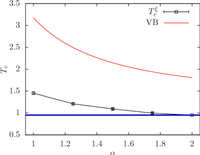
Figure 6: (Color online) Critical temperature $T_{c}$ computed from a finite-size scaling of the two-point correlation length, Eq. (7), using the extended scaling technique, Eq. (9). The continuous curve (labeled with VB) is the critical temperature $T_{c}$ for a mean-field spin glass on a diluted graph with fixed connectivity $k+1=6$. The horizontal thick line represents the critical temperature $T_{c}$ for the Gaussian spin glass.Katzgraber et al. (2006)

V Conclusions

We have studied the critical behavior of a three-dimensional Ising spin glass with Lévy-distributed interactions to test universality. An extended scaling analysis of the correlation length and spin-glass susceptibility suggests that for all values of $\alpha$ the Lévy spin glass obeys universality. Previous claims that universality might be destroyed when $\alpha\to 1$ possibly stem from the fact that the simulations did not take into account the effects of the strong interactions between some spins, i.e., rendering the simulations nonergodic. Further support for universal behavior is given by the plot of $g$ against $\xi_{L}/L$, Fig. 5, where data for all the models studied collapse onto a single universal curve. We do find strong corrections to scaling and therefore studies with larger system sizes and a clear understanding of scaling corrections would be desirable. However, we find no clear evidence for the lack of universality.